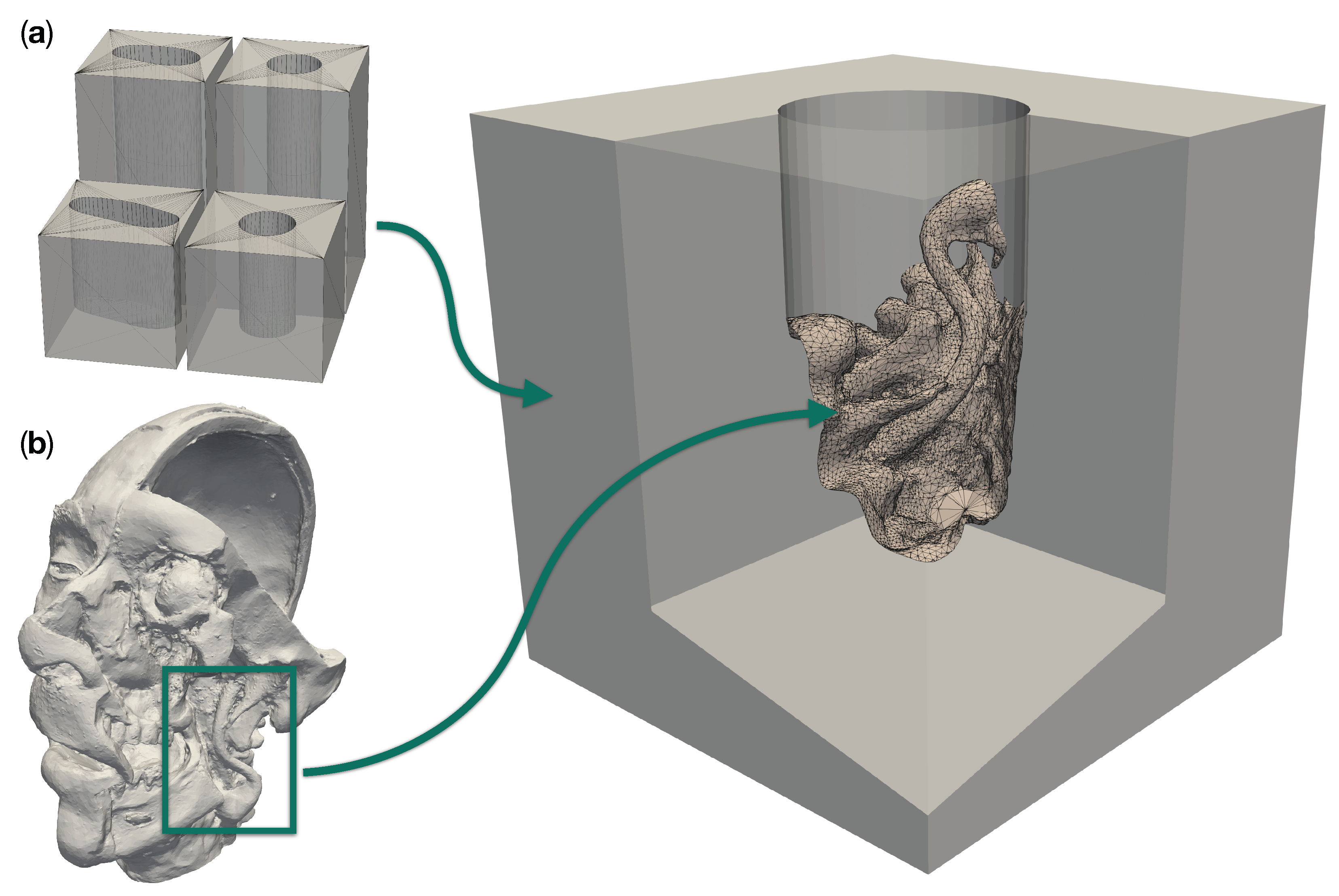
Figure 1.
Design components for a realistic site models with a patient anatomy in a deep operative corridors. (a) shows the four different operative corridors used: Two cylindrical channels with a depth of 50 and 100 , respectively, as well as two channels of the same depths with a deformed elliptical cross-section. (b) Three-dimensional model of a plastinated and dissected human head. The box highlights the region which was merged into an empty cylindrical channel to create the particular model to the right.
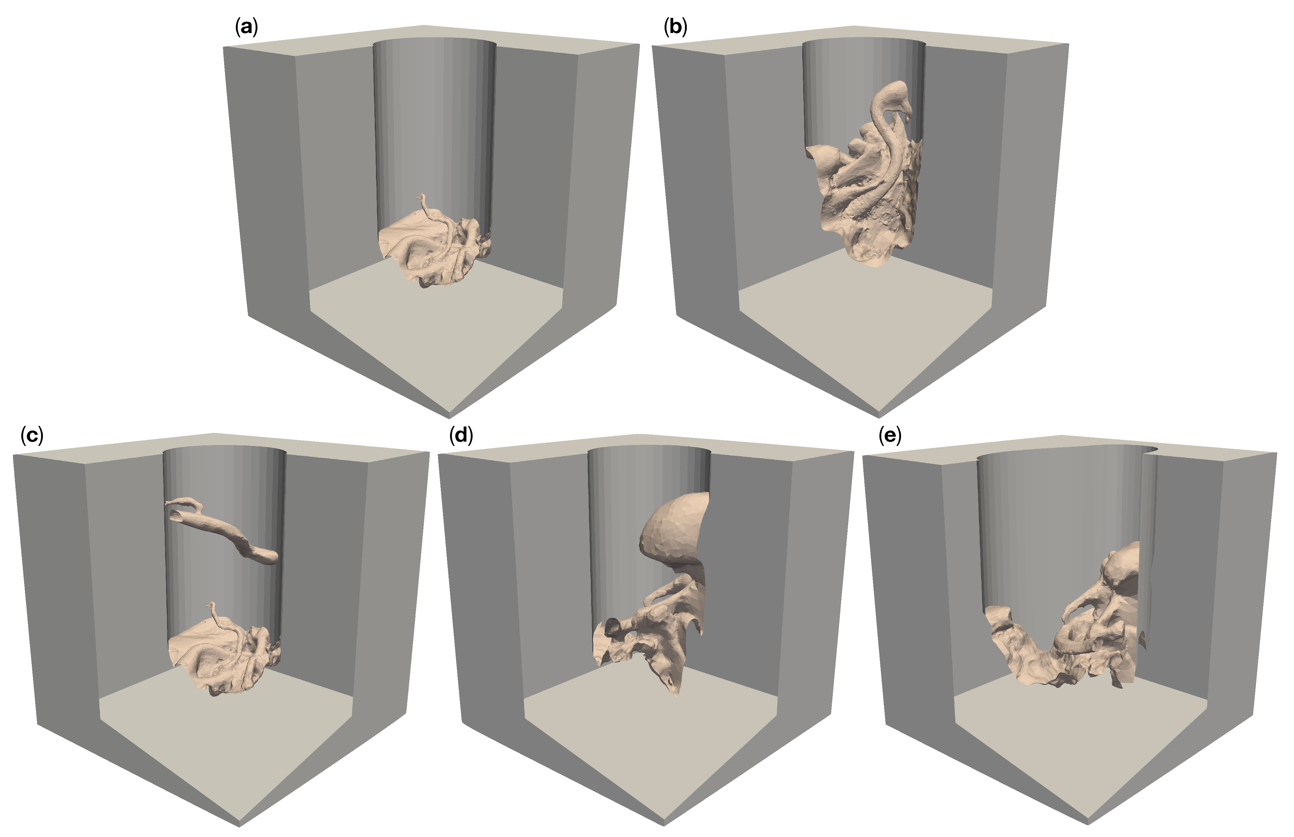
Figure 2.
Five different artificial patient surgical site models with a 50 deep operative corridors. “Circ flat anatomy”, shown in (a), contains a rather flat topology. “Circ angled anatomy” in (b) features a network of arteries, tissue furrows and undercuts, which are set at an angle in the corridor. “Circ artery” (c) has the same flat topology as in (a) at the bottom of the operative corridor, but adds an artery spanning the operative corridor. (d) shows a topology consisting of a mixture of arteries, tissue furrows, undercuts, dominated by a large overhang protruding from the channel wall. This model is called “circ overhang”. The model in (e) combines features from (b,d), set in an operating corridor with deformed elliptical cross-section, hence its name: “elliptical channel”.
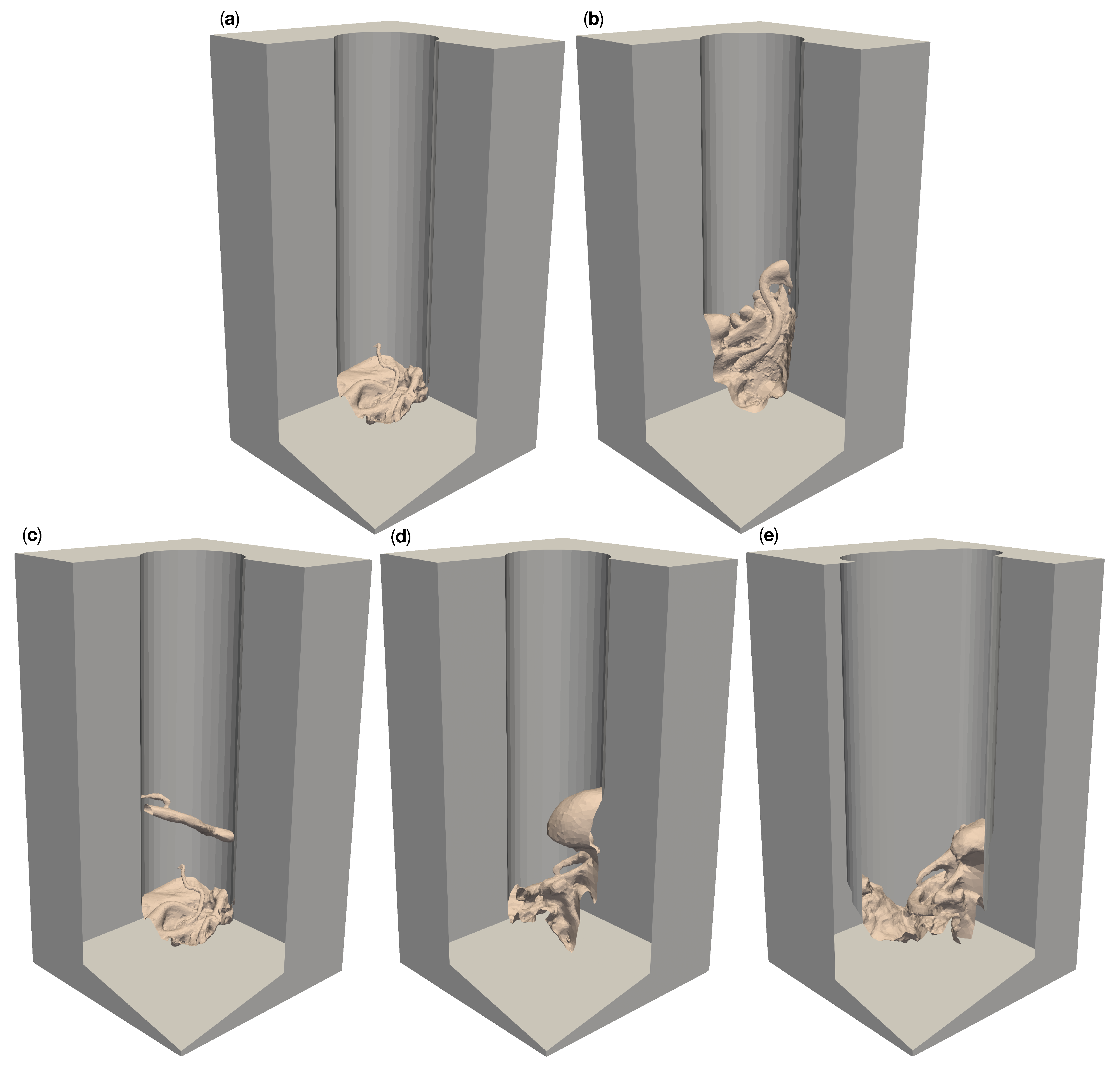
Figure 3.
Five different artificial patient surgical site models with 100 deep operative corridors. “Circ flat anatomy”, shown in (a), contains a rather flat topology. “Circ angled anatomy” in (b) features a network of arteries, tissue furrows and undercuts, which are set at an angle in the corridor. “Circ artery” (c) has the same flat topology as in (a) at the bottom of the operative corridor but adds an artery spanning the operative corridor. (d) shows a topology consisting of a mixture of arteries, tissue furrows, undercuts, dominated by a large overhang protruding from the channel wall. This model is called “circ overhang”. The model in (e) combines features from (b,d), set in an operating corridor with a deformed elliptical cross-section, hence its name: “elliptical channel”.
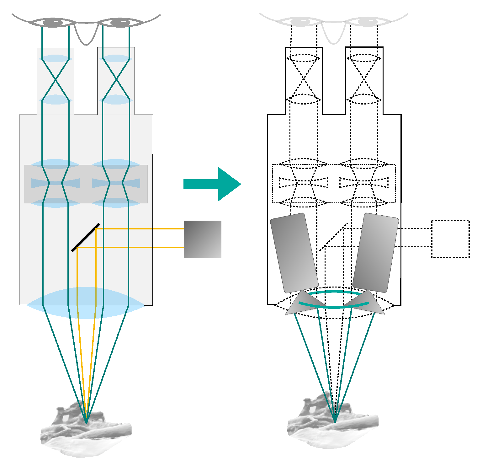
Figure 4.
Simplifications used in our surgical microscope model. The optical setup within the microscope is omitted and the main objective lens is assumed to be ideal. The cameras are placed directly on the non-refracted ray paths, at a distance from the object equal to the focal length of the main objective lens. The cameras are located on a ring with the diameter of the CMO lens (shown in green).
Figure 5.
Schematic of the final camera setup model with an example mesh and four cameras. The mesh is centered at the origin of the world coordinate system. The cameras are placed on a ring (green) above the mesh. The wireframe hemisphere lies at a distance from the origin equal to the common main objective lens’ focal length. It marks the surface on which cameras may be positioned. The optical axes of the cameras are shown in red. The cameras all “look at” the central reference point, which is the origin in this case. The figure is not to scale in the z-direction. It has been shortened for illustration purposes.
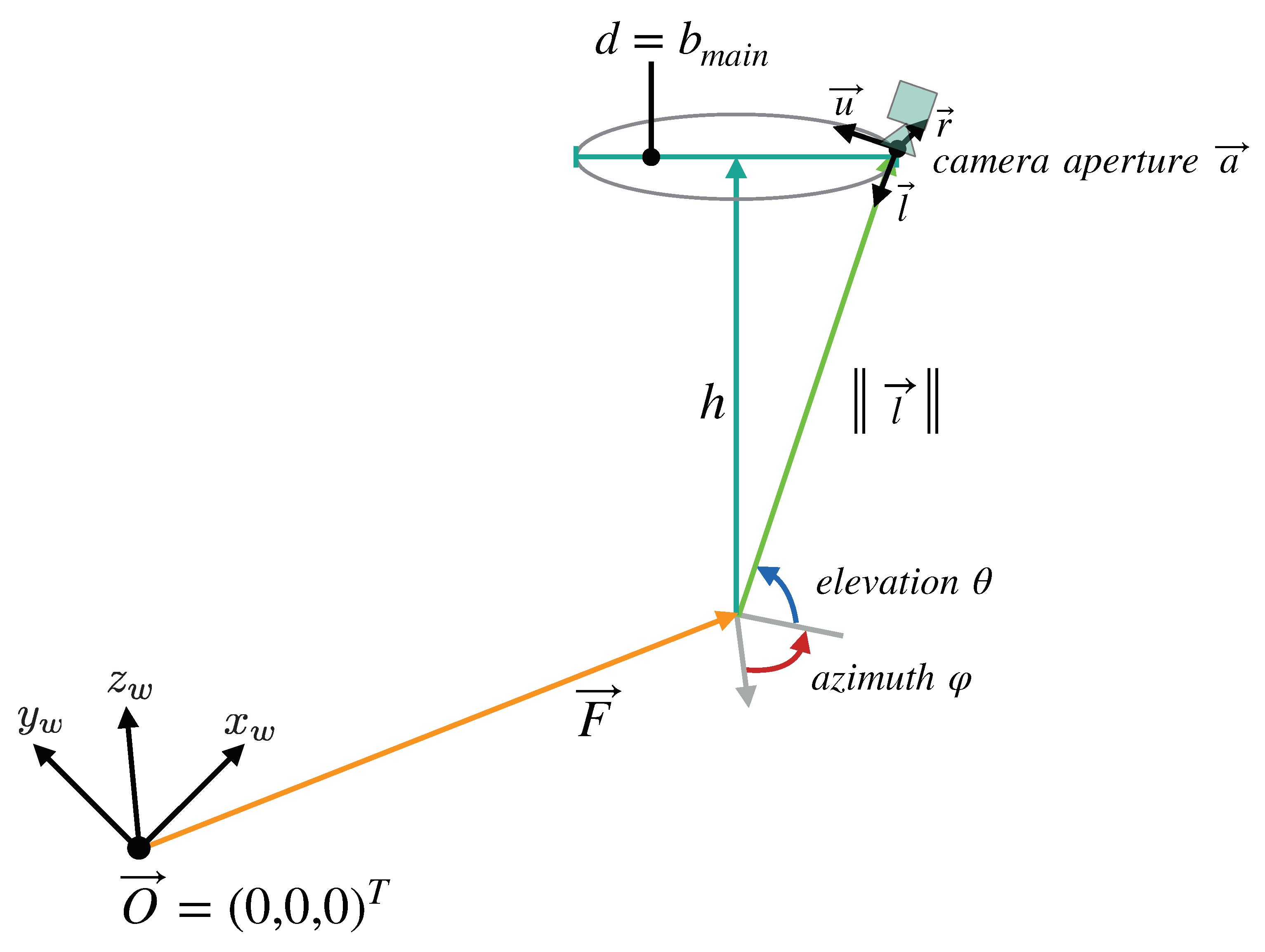
Figure 6.
Overview of the parameters that define the camera setup model we devised for our simulation. The cameras lie on a ring with the diameter d, at the distance h from the reference point , which all cameras look at. The distance h is equivalent to the working distance of the fully digital microscope simulated by the model, while d is the maximum baseline allowed by the microscope’s main objective. The points on the ring can be described in spherical coordinates relative to . In these coordinates, is equal to the main objective’s focal length.
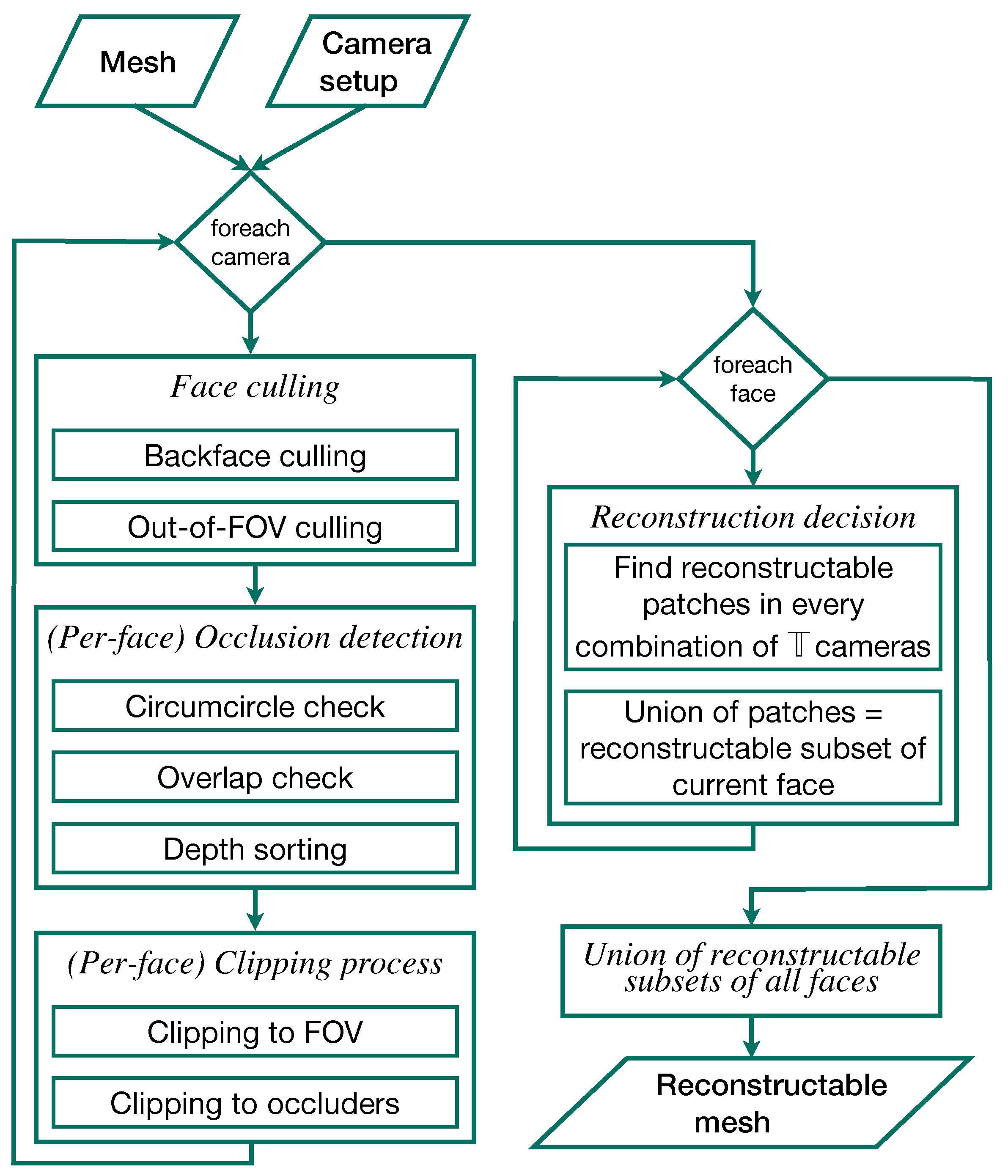
Figure 7.
Overview flow chart of the individual steps of the 3D reconstruction simulation. The camera setup and surgical site models comprise the input. The output is the reconstructable subset of the input mesh in 3D.
Figure 7.
Overview flow chart of the individual steps of the 3D reconstruction simulation. The camera setup and surgical site models comprise the input. The output is the reconstructable subset of the input mesh in 3D.
Figure 8.
Overlay plots of the 3D reconstructable surfaces of the five different 50 -channel surgical site models for different camera numbers. The reconstruction with the largest area was placed in the background and the reconstruction with the smallest area in the foreground. The areas are color coded by number of cameras: Gray for two cameras, red for four cameras, orange for six, yellow for eight, lime for 16, green for 32, cyan for 64, blue for 128, purple for 256, and magenta for 360. (a) shows the reconstruction of “circ flat anatomy”. (b) does this for “circ angled anatomy”, (c) for “circ artery”, (d) for “circ overhang”, and (e) for the “elliptical channel” mesh.
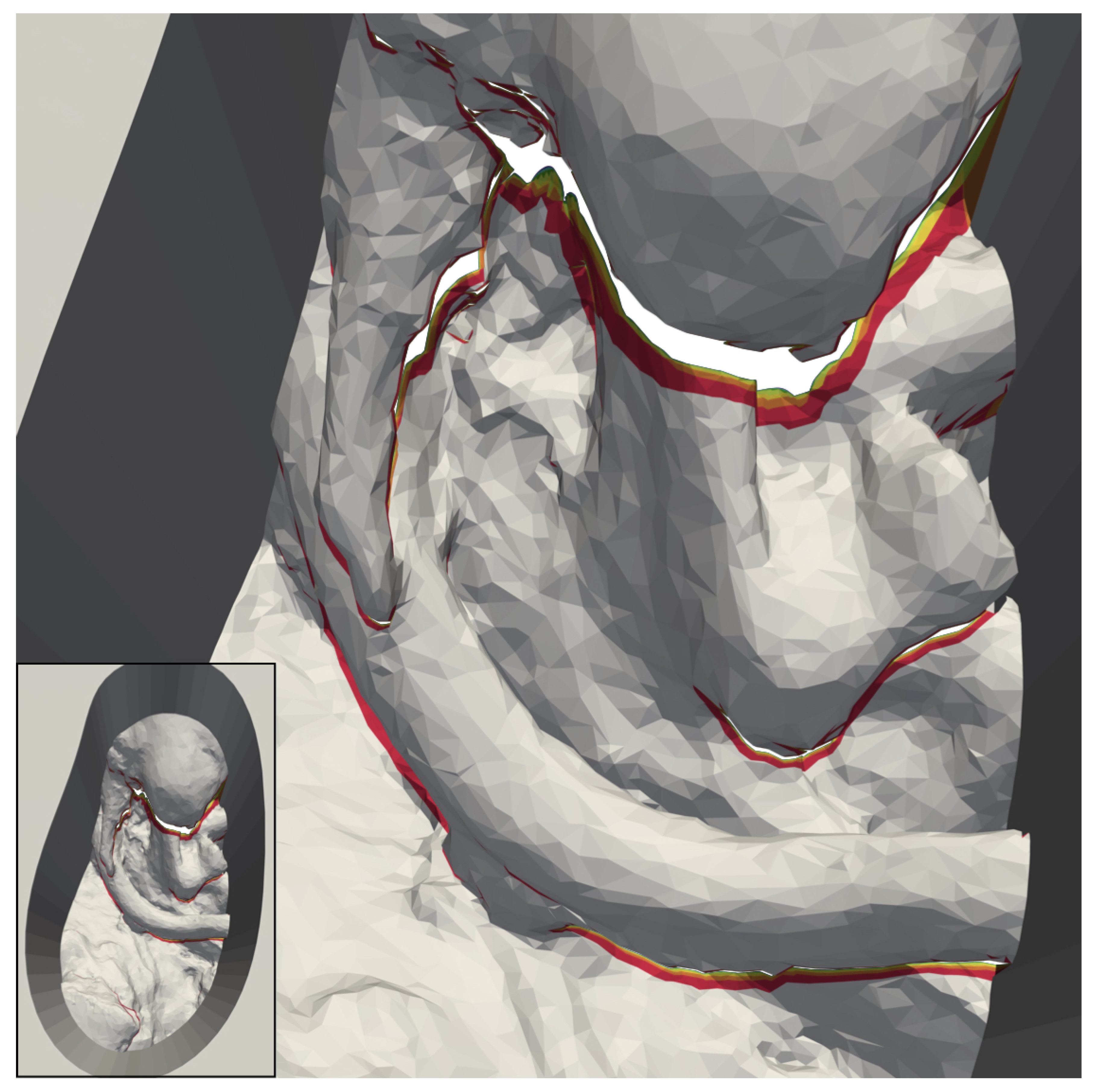
Figure 9.
Magnified images of the 3D reconstructable surface of the model “circ artery”. The reconstruction with the largest area was placed in the background and the reconstruction with the smallest area in the foreground. (a) shows that the reconstructable area towards the outside of the top surface increases noticeably up to 128 cameras. After that, the increase is difficult to visually. (b) shows part of the model in which a vessel with a branch obscures the anatomy below. Large portions of this area are not reconstructable with two cameras (gray). In contrast to this, with four cameras, the red portions become available. The areas in different colors represents additional areas reconstructable with six (orange), eight (yellow), 16 (lime), 32 (green), 64 (cyan), 128 (blue), 256 (purple), and 360 (magenta) cameras.
Figure 10.
Overlay of zoomed plots of the 3D reconstructable surfaces of the five different 100 -channel surgical site models for different camera numbers. The reconstruction with the largest area was placed in the background and the reconstruction with the smallest area in the foreground. The areas are color coded by number of cameras: Gray for two cameras, red for four cameras, orange for six, yellow for eight, lime for 16, green for 32, cyan for 64, blue for 128, purple for 256, and magenta for 360. (a) shows the reconstruction of “circ flat anatomy”. (b) does this for “circ angled anatomy”, (c) for “circ artery”, (d) for “circ overhang”, and (e) for the “elliptical channel” mesh.
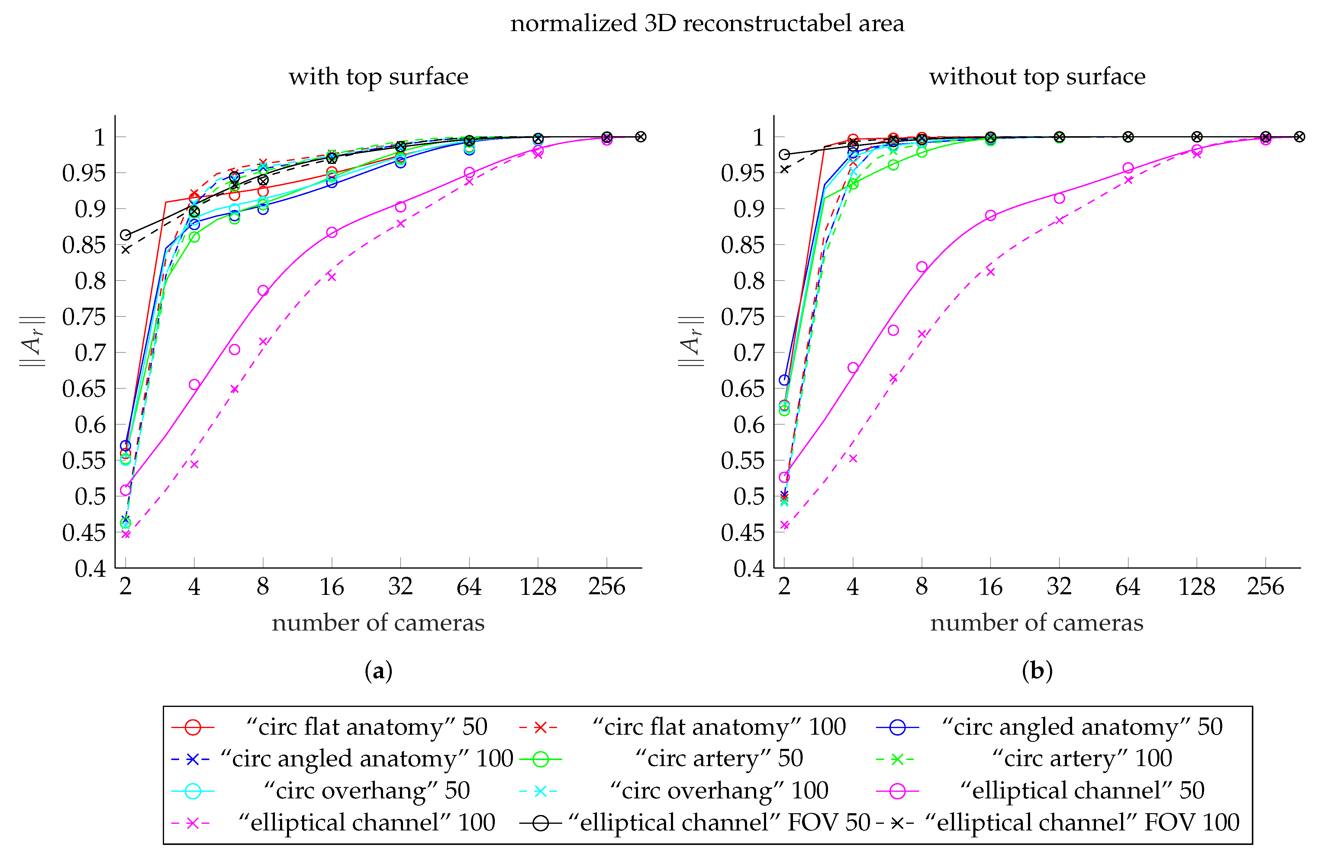
Figure 11.
Comparison plot showing the fit functions to the reconstructable area values for each of our meshes. (a) shows the fit functions including the top surface, (b) shows the fits to data excluding the top surface. The curves for the meshes with 50 deep channel are solid lines. The dashed lines shows the curves of the meshes with 100 deep channel. The colors red, blue, green, and cyan represent the meshes “circ flat anatomy”, “circ angled anatomy”, “circ artery”, and “circ overhang”, in this order. Magenta belongs to the elliptical channel models, using the smaller FOV. The black curves belong to elliptical channel fits with larger FOV. The scattered markers represent the measured area values.
Figure 12.
Reconstructable subset of the 50 deep version of our “elliptical channel” model, using cameras with increased FOV size. The regions shown in grey are reconstructable with only two cameras. The area added by four cameras is red. In addition, shown are additional areas reconstructable with six (orange), eight (yellow), 16 (lime), and 32 (green) cameras.
Table 1.
Operation channel diameters for groups of lesions that are of particular interest in microsurgery. We used these values as a basis for the design of our operation channel models. All values are given in millimeters. Data provided by Carl ZEISS Meditec AG.
Table 1.
Operation channel diameters for groups of lesions that are of particular interest in microsurgery. We used these values as a basis for the design of our operation channel models. All values are given in millimeters. Data provided by Carl ZEISS Meditec AG.
| Organ | Operation Type | Diameter Range | Average Diameter | Depth Range |
|---|
| Brain | Glioblastoma resection | 40–70 | 55 | 40–90 |
| Interventions in the cerebellopontine angle | 20–40 | 30 | 60–100 |
| Spine | Intervertebral disc surgery | 20–30 | 25 | 50–100 |
Table 2.
Reconstructable areas () of the 50 channel models for different numbers of cameras, including the top surface. The area values for each mesh are normalized to the area of the respective mesh which is reconstructable with 360 cameras. denotes the increase in reconstructable area from the next smaller number of cameras.
| Number of | “Circ Flat Anatomy” | “Circ Angled Anatomy” | “Circ Artery” | “Circ Overhang” | “Elliptical Channel” |
|---|
| Cameras | | | | | | | | | | |
|---|
| 2 | 0.5595 | 0 | 0.5703 | 0 | 0.5519 | 0 | 0.5501 | 0 | 0.5084 | 0 |
| 4 | 0.9142 | 0.3548 | (+63.41%) | 0.8778 | 0.3076 | (+53.93%) | 0.8604 | 0.3085 | (+55.9%) | 0.8844 | 0.3343 | (+60.77%) | 0.6554 | 0.1469 | (+28.9%) |
| 6 | 0.9185 | 0.0043 | (+0.47%) | 0.8902 | 0.0124 | (+1.41%) | 0.8858 | 0.0253 | (+2.94%) | 0.8995 | 0.0151 | (+1.71%) | 0.704 | 0.0487 | (+7.43%) |
| 8 | 0.9239 | 0.0054 | (+0.59%) | 0.8990 | 0.0088 | (+0.99%) | 0.9054 | 0.0197 | (+2.22%) | 0.9098 | 0.0102 | (+1.14%) | 0.7861 | 0.0821 | (+11.66%) |
| 16 | 0.9511 | 0.0272 | (+2.94%) | 0.9363 | 0.0373 | (+4.15%) | 0.9461 | 0.0406 | (+4.49%) | 0.9437 | 0.034 | (+3.73%) | 0.867 | 0.0809 | (+10.29%) |
| 32 | 0.9719 | 0.0208 | (+2.19%) | 0.9638 | 0.0275 | (+2.94%) | 0.9701 | 0.0241 | (+2.54%) | 0.9681 | 0.0244 | (+2.58%) | 0.9025 | 0.0355 | (+4.09%) |
| 64 | 0.9857 | 0.0138 | (+1.42%) | 0.9817 | 0.0179 | (+1.85%) | 0.9851 | 0.0149 | (+1.54%) | 0.9838 | 0.0157 | (+1.62%) | 0.9503 | 0.0478 | (+5.3%) |
| 128 | 0.9963 | 0.0106 | (+1.08%) | 0.9952 | 0.0135 | (+1.38%) | 0.9961 | 0.011 | (+1.12%) | 0.9958 | 0.012 | (+1.22%) | 0.9807 | 0.0304 | (+3.2%) |
| 256 | 0.999 | 0.0027 | (+0.27%) | 0.9988 | 0.0035 | (+0.35%) | 0.999 | 0.0029 | (+0.29%) | 0.9989 | 0.0031 | (+0.31%) | 0.9955 | 0.0148 | (+1.51%) |
| 360 | 1 | 0.001 | (+0.1%) | 1 | 0.0012 | (+0.12%) | 1 | 0.001 | (+0.1%) | 1 | 0.0011 | (+0.11%) | 1 | 0.0045 | (+0.46%) |
Table 3.
Reconstructable areas () of the 100 channel models for different numbers of cameras, including the top surface. The area values for each mesh are normalized to the area of the respective mesh which is reconstructable with 360 cameras. denotes the increase in reconstructable area from the next smaller number of cameras.
| Number of | “Circ Flat Anatomy” | “Circ Angled Anatomy” | “Circ Artery” | “Circ Overhang” | “Elliptical Channel” |
|---|
| Cameras | | | | | | | | | | |
|---|
| 2 | 0.4673 | 0 | 0.4674 | 0 | 0.4629 | 0 | 0.4593 | 0 | 0 | 0.4474 | 0 | 0 |
| 4 | 0.9214 | 0.4541 | (+97.19%) | 0.9044 | 0.437 | (+93.49%) | 0.8942 | 0.4314 | (+93.19%) | 0.9072 | 0.4479 | (+97.52%) | 0.5443 | 0.0969 | (+21.65%) |
| 6 | 0.9494 | 0.028 | (+3.04%) | 0.9396 | 0.0352 | (+3.89%) | 0.9313 | 0.0371 | (+4.15%) | 0.9428 | 0.0356 | (+3.92%) | 0.6493 | 0.105 | (+19.29%) |
| 8 | 0.9641 | 0.0147 | (+1.55%) | 0.9571 | 0.0175 | (+1.86%) | 0.9547 | 0.0234 | (+2.51%) | 0.9595 | 0.0168 | (+1.78%) | 0.7153 | 0.066 | (+10.16%) |
| 16 | 0.9767 | 0.0126 | (+1.31%) | 0.9728 | 0.0156 | (+1.64%) | 0.9741 | 0.0195 | (+2.04%) | 0.9746 | 0.015 | (+1.57%) | 0.8049 | 0.0896 | (+12.52%) |
| 32 | 0.986 | 0.0093 | (+0.95%) | 0.9839 | 0.0111 | (+1.14%) | 0.9851 | 0.011 | (+1.13%) | 0.9849 | 0.0104 | (+1.07%) | 0.8792 | 0.0743 | (+9.23%) |
| 64 | 0.9929 | 0.0069 | (+0.7%) | 0.9919 | 0.0081 | (+0.82%) | 0.9927 | 0.0075 | (+0.77%) | 0.9925 | 0.0075 | (+0.76%) | 0.9375 | 0.0583 | (+6.63%) |
| 128 | 0.9976 | 0.0047 | (+0.47%) | 0.9973 | 0.0053 | (+0.54%) | 0.9975 | 0.0048 | (+0.49%) | 0.9975 | 0.005 | (+0.5%) | 0.9749 | 0.0374 | (+3.99%) |
| 256 | 0.9993 | 0.0017 | (+0.17%) | 0.9992 | 0.0019 | (+0.19%) | 0.9993 | 0.0018 | (+0.18%) | 0.9993 | 0.0018 | (+0.18%) | 0.9944 | 0.0195 | (+2%) |
| 360 | 1 | 0.0007 | (+0.07%) | 1 | 0.0008 | (+0.08%) | 1 | 0.0007 | (+0.07%) | 1 | 0.0007 | (+0.07%) | 1 | 0.0056 | (+0.57%) |
Table 4.
Reconstructable areas () of the 50 channel models for different numbers of cameras, excluding the top surface. The area values for each mesh are normalized to the area of the respective mesh which is reconstructable with 360 cameras. denotes the increase in reconstructable area from the previous smaller number of cameras.
| Number of | “Circ Flat Anatomy” | “Circ Angled Anatomy” | “Circ Artery” | “Circ Overhang” | “Elliptical Channel” |
|---|
| Cameras | | | | | | | | | | |
|---|
| 2 | 0.6264 | 0 | 0.6615 | 0 | 0.619 | 0 | 0.6249 | 0 | 0.5263 | 0 |
| 4 | 0.9965 | 0.37 | (+59.07%) | 0.9776 | 0.3161 | (+47.79%) | 0.9343 | 0.3153 | (+50.94%) | 0.9723 | 0.3474 | (+55.6%) | 0.6788 | 0.1525 | (+28.99%) |
| 6 | 0.9979 | 0.0014 | (+0.15%) | 0.9883 | 0.0107 | (+1.09%) | 0.9608 | 0.0265 | (+2.83%) | 0.9865 | 0.0142 | (+1.46%) | 0.7308 | 0.052 | (+7.66%) |
| 8 | 0.9989 | 0.001 | (+0.1%) | 0.9921 | 0.0038 | (+0.39%) | 0.9786 | 0.0178 | (+1.86%) | 0.9927 | 0.0062 | (+0.63%) | 0.8191 | 0.0883 | (+12.09%) |
| 16 | 0.9996 | 0.0007 | (+0.07%) | 0.9968 | 0.0047 | (+0.47%) | 0.9947 | 0.0161 | (+1.64%) | 0.9977 | 0.005 | (+0.5%) | 0.8906 | 0.0715 | (+8.73%) |
| 32 | 0.9999 | 0.0003 | (+0.03%) | 0.9989 | 0.002 | (+0.21%) | 0.9984 | 0.0037 | (+0.37%) | 0.9994 | 0.0016 | (+0.16%) | 0.9144 | 0.0238 | (+2.67%) |
| 64 | 0.9999 | 0.0001 | (+0.01%) | 0.9996 | 0.0007 | (+0.07%) | 0.9995 | 0.0011 | (+0.11%) | 0.9998 | 0.0004 | (+0.04%) | 0.9567 | 0.0423 | (+4.62%) |
| 128 | 1 | 0 | (+0%) | 0.9998 | 0.0003 | (+0.03%) | 0.9998 | 0.0003 | (+0.03%) | 0.9999 | 0.0001 | (+0.01%) | 0.9817 | 0.025 | (+2.61%) |
| 256 | 1 | 0 | (+0%) | 1 | 0.0001 | (+0.01%) | 1 | 0.0002 | (+0.02%) | 1 | 0.0001 | (+0.01%) | 0.9958 | 0.0141 | (+1.44%) |
| 360 | 1 | 0 | (+0%) | 1 | 0 | (+0%) | 1 | 0 | (+0%) | 1 | 0 | (+0%) | 1 | 0.0042 | (+0.42%) |
Table 5.
Reconstructable areas () of the 100 channel models for different numbers of cameras, excluding the top surface. The area values for each mesh are normalized to the area of the respective mesh which is reconstructable with 360 cameras. denotes the increase in reconstructable area from the next smaller number of cameras.
| Number of | “Circ Flat Anatomy” | “Circ Angled Anatomy” | “Circ Artery” | “Circ Overhang” | “Elliptical Channel” |
|---|
| Cameras | | | | | | | | | | |
|---|
| 2 | 0.4978 | 0 | 0.502 | 0 | 0.4934 | 0 | 0.4911 | 0 | 0.4604 | 0 |
| 4 | 0.9645 | 0.4668 | (+93.77%) | 0.9519 | 0.4499 | (+89.62%) | 0.9359 | 0.4425 | (+89.67%) | 0.9519 | 0.4608 | (+93.85%) | 0.5525 | 0.092 | (+19.99%) |
| 6 | 0.999 | 0.0344 | (+3.57%) | 0.9949 | 0.043 | (+4.52%) | 0.9801 | 0.0443 | (+4.73%) | 0.9949 | 0.043 | (+4.51%) | 0.6649 | 0.1125 | (+20.36%) |
| 8 | 0.9995 | 0.0005 | (+0.05%) | 0.9966 | 0.0017 | (+0.17%) | 0.9898 | 0.0096 | (+0.98%) | 0.9967 | 0.0019 | (+0.19%) | 0.7257 | 0.0608 | (+9.14%) |
| 16 | 0.9999 | 0.0004 | (+0.04%) | 0.9986 | 0.002 | (+0.2%) | 0.9974 | 0.0076 | (+0.77%) | 0.9989 | 0.0022 | (+0.22%) | 0.8121 | 0.0864 | (+11.9%) |
| 32 | 1 | 0.0001 | (+0.01%) | 0.9995 | 0.0009 | (+0.09%) | 0.9992 | 0.0018 | (+0.18%) | 0.9997 | 0.0007 | (+0.07%) | 0.8838 | 0.0717 | (+8.83%) |
| 64 | 1 | 0 | (+0%) | 0.9998 | 0.0003 | (+0.03%) | 0.9998 | 0.0006 | (+0.06%) | 0.9999 | 0.0002 | (+0.02%) | 0.9398 | 0.0561 | (+6.34%) |
| 128 | 1 | 0 | (+0%) | 0.9999 | 0.0001 | (+0.01%) | 0.9999 | 0.0001 | (+0.01%) | 1 | 0.0001 | (+0.01%) | 0.9755 | 0.0357 | (+3.79%) |
| 256 | 1 | 0 | (+0%) | 1 | 0 | (+0%) | 1 | 0.0001 | (+0.01%) | 1 | 0 | (+0%) | 0.9946 | 0.0191 | (+1.96%) |
| 360 | 1 | 0 | (+0%) | 1 | 0 | (+0%) | 1 | 0 | (+0%) | 1 | 0 | (+0%) | 1 | 0.0054 | (+0.54%) |
Table 6.
Reconstructable areas () of the “elliptical channel” models for different numbers of cameras using an larger FOV (60 × 60 ). The area values for each mesh are normalized to the area of the respective mesh which is reconstructable with 360 cameras. denotes the increase in reconstructable area from the next smaller number of cameras.
| Number of Cameras | Elliptical Channel with a Larger FOV |
|---|
| Including Top Surface | Excluding Top Surface |
|---|
| 50 mm Deep Channels | 100 mm Deep Channels | 50 mm Deep Channels | 100 mm Deep Channels |
|---|
| | | | | | | |
|---|
| 2 | 0.8634 | 0 | 0.8427 | 0 | 0.9752 | 0 | 0.9547 | 0 |
| 4 | 0.8959 | 0.0324 | (+3.76%) | 0.8966 | 0.0538 | (+6.39%) | 0.987 | 0.0118 | (+1.21%) | 0.9932 | 0.0385 | (+4.03%) |
| 6 | 0.944 | 0.0481 | (+5.37%) | 0.9334 | 0.0369 | (+4.11%) | 0.9933 | 0.0062 | (+0.63%) | 0.9965 | 0.0033 | (+0.33%) |
| 8 | 0.94 | −0.004 | (−0.42%) | 0.9375 | 0.0041 | (+0.44%) | 0.996 | 0.0027 | (+0.28%) | 0.9979 | 0.0014 | (+0.14%) |
| 16 | 0.9699 | 0.0299 | (+3.18%) | 0.9675 | 0.03 | (+3.2%) | 0.999 | 0.003 | (+0.3%) | 0.9995 | 0.0016 | (+0.16%) |
| 32 | 0.9862 | 0.0163 | (+1.68%) | 0.9884 | 0.0209 | (+2.16%) | 0.9996 | 0.0006 | (+0.06%) | 0.9998 | 0.0003 | (+0.03%) |
| 64 | 0.9944 | 0.0082 | (+0.83%) | 0.9937 | 0.0053 | (+0.54%) | 0.9998 | 0.0002 | (+0.02%) | 0.9999 | 0.0001 | (+0.01%) |
| 128 | 0.9975 | 0.0031 | (+0.31%) | 0.9977 | 0.004 | (+0.4%) | 0.9999 | 0.0001 | (+0.01%) | 1 | 0 | (+0%) |
| 256 | 0.9995 | 0.002 | (+0.2%) | 0.9992 | 0.0015 | (+0.15%) | 1 | 0 | (+0%) | 1 | 0 | (+0%) |
| 360 | 1 | 0.0005 | (+0.05%) | 1 | 0.0008 | (+0.080%) | 1 | 0 | (+0%) | 1 | 0 | (+0%) |


