
Postprocessing for Skin Detection


1
Department of Information Engineering (DEI), University of Padova, 35131 Padova, Italy
2
Department of Information Technology and Cybersecurity, Missouri State University, Springfield, MO 65804, USA
3
Department of Computer Science and Engineering (DISI), University of Bologna, 47521 Cesena, Italy
*
Author to whom correspondence should be addressed.
J. Imaging 2021, 7(6), 95; https://0-doi-org.brum.beds.ac.uk/10.3390/jimaging7060095
Submission received: 21 April 2021
/
Revised: 24 May 2021
/
Accepted: 28 May 2021
/
Published: 3 June 2021
Abstract
:Skin detectors play a crucial role in many applications: face localization, person tracking, objectionable content screening, etc. Skin detection is a complicated process that involves not only the development of apposite classifiers but also many ancillary methods, including techniques for data preprocessing and postprocessing. In this paper, a new postprocessing method is described that learns to select whether an image needs the application of various morphological sequences or a homogeneity function. The type of postprocessing method selected is learned based on categorizing the image into one of eleven predetermined classes. The novel postprocessing method presented here is evaluated on ten datasets recommended for fair comparisons that represent many skin detection applications. The results show that the new approach enhances the performance of the base classifiers and previous works based only on learning the most appropriate morphological sequences.
1. Introduction
A highly relevant segmentation problem is skin detection, a problem that discriminates regions in images and videos into the two classes skin and nonskin. The applications of skin detection are many, as are the challenges. Skin detection is a valuable component in locating faces, tracking individuals, human–computer interactions, biometric authentication, medical imaging, and objectionable content screening [1]. Challenges are concerned not only with building powerful classifiers but also with developing all the additional methods required to accomplish the task, including data preprocessing and postprocessing.
When discussing the history of a machine learning problem, it is often appropriate to divide developments into two periods: those before and those after the rise of deep learning. Prior to deep learning, most human skin detection approaches were based either on skin color separation or texture features. Skin color separation assumes that skin tones can be distinguished from background colors via a clustering rule in a color space [2]. A survey of the literature comparing different color spaces is available in reference [3]. The authors in that review surveyed four types of color models: (1) basic color models like RGB and normalized RGB, (2) perceptual models like HIS and HSV, (3) perceptual uniform models like CIE-Lab and CIE-Luv, and (4) orthogonal models like YCbCr and YIQ. A more challenging way to tackle skin detection is to assume a nonconstrained environment [3]; this type of approach involves training classifiers that have the capacity to generalize. Some skin segmentation examples along this line include using a multilayer perceptron [4], random forest [5], Bayesian classifiers [6], and adaptive discriminative analysis [7]. Another class of early approaches relies on image segmentation, where pixel neighborhoods are examined to segment regions where human skin is located [8,9].
Developments in skin detection in the deep learning age often involve applying Convolutional Neural Networks (CNN) to skin segmentation. CNNs are well-known for their superior performance in image classification and in segmentation tasks involving pixel-based prediction like scene labeling. One of the first works to apply deep learning to human skin detection was reference [10], where patch-based networks trained on a dataset of patches were shown to compete well with pixel-wise classification. Later, in reference [11], a procedure for human skin detection was designed that combined recurrent neural network (RNN) layers with fully CNN (FCN). The advantage of this combination was that the FCN layers captured local features while the RNN layers modeled the semantic contextual dependencies. In reference [12], an inception-based architecture was proposed that was composed of convolutional and inception modules with training considering both patches and whole images. In reference [13], the authors performed experiments using several CNN architectures and concluded that DeepLabv3+ is the best CNN for skin segmentation. Two very recent skin segmentation architectures are OR-Skip-Net [14], a model that transfers direct edge information across the network in such a way as to empower the features, and Skinny [15], based on a lightweight U-Net. A deep learning approach based on transfer learning was proposed in reference [16] for skin detection in gray-scale images; this model is based on the combination of a colorization network and a pretrained Inception-ResNet-v2.
Several studies have been conducted that provide comprehensive evaluations of CNN architectures with the intention of finding the most promising ones [13,17,18]. For example, in reference [17], an extensive evaluation was conducted that compared the best pixel-based methods with CNN approaches both in-domain and cross-domain. In reference [18], experiments were performed on many different CNN structures in an attempt to isolate those that work best for skin detection. Besides providing an exhaustive comparison of skin color detection approaches, the authors in reference [13] developed a framework for fair comparisons of methods in skin detection. The advantages of using deep learning methods for skin detection (as compared with pixel-based and classical region-based approaches) were demonstrated in the experiments performed in references [13,17].
The results from comprehensive evaluations of both CNN architectures and handcrafted methods have revealed much room for performance improvement, mainly when it comes to low-quality input images where postprocessing is often required to improve the segmentation performance. In the literature, several postprocessing ideas have been proposed to improve the performance of skin segmentation. In reference [19], for example, a simple rejection rule was developed to remove small noisy regions from the final mask, while, in reference [20], an adaptive method based on a blob analysis was proposed to improve the classification performance of color-based skin detectors. The methods designed for pixel-based segmentation approaches, which classify every pixel separately, can produce high false positives for background pixels when the color is too similar to human skin. Deep learning approaches do not suffer from these problems since they are based on a global analysis of the image. A recent work [21] has suggested the application of learned morphological operators to improve the performance of deep learners in skin detection. In learned postprocessing, a classifier learns the best postprocessing method to use based on the type of image under consideration.
In this paper, a new learned postprocessing method for skin detection is proposed that applies either a set of morphological processes or a homogeneity function. Mathematical morphologies provides powerful nonlinear operators for a variety of image processing tasks, such as filtering, segmentation, and edge detection. In some recent works, novel morphological layers have been proposed to include learned morphological operators inside a deep learning framework, mainly for applications of image classification, denoising, edge detection, or super-resolution [22,23]. In this study, as in reference [21], which this work extends, skin is detected, first, by segmenting the image with a deep learner (or another handcrafted approach) and, second, by applying a postprocessing method. This approach involves classifying an image into several classes (predetermined by the researchers) that govern which postprocessing method to apply. Therefore, in this work, the postprocessing step is based on handcrafted processes, while a learning procedure is used to select the appropriate approach. In reference [21], five image classes were identified for using different sets of morphological processes. Here, eleven classes have been identified. The collection of possible postprocessing methods includes not only the morphological processes but, also, a homogeneity function. The main aim of this work is to find a criterion for selecting images that need a homogeneity postprocessing method instead of a morphological approach.
Following the testing framework developed in reference [13], the performance results of the learning procedure proposed here to select the appropriate postprocessing functions (either morphological or homogeneity) are compared to several state-of-the-art detectors without postprocessing and to the results produced by the postprocessing methods proposed in reference [21]. A series of experiments demonstrate that the novel postprocessing method improves the detection across several datasets representing different applications and is superior to that introduced in reference [21]. Additionally, several training protocols are examined that show the usefulness of a learned postprocessing approach, even without specific training on the datasets.
The remainder of this paper is organized as follows. In Section 2, the general approach for learning the best method to take in the postprocessing phase is described. This section includes a discussion of CNN fine-tuning for skin detection. In Section 3, the testing framework for comparing skin detection systems is described, and a set of experiments are presented that demonstrate the ability of the proposed postprocessing method to boost the performance of state-of-the-art skin detectors. This paper concludes in Section 4 by offering some directions for further research.
2. System Description
2.1. Skin Detection with Deep Learners
The application of deep learning to the general problem of segmentation is relatively recent [24], and, as happened in other applications, it immediately outperformed the previous state-of-the-art approaches based on handcrafted methods. Long et al. [25] were among the first to adapt deep learners (AlexNet and GoogLeNet) to the task of segmentation by fine-tuning the FCN layers of these deep learners. Another powerful deep learner tailored for image segmentation is the encoding/decoding network SegNet [26]. The encoder part of SegNet is the same as the convolutional layers in the VGG16 network [27]. In SegNet, each of the thirteen encoders is coupled with a decoder. As weights can be trained for classification on larger datasets, the FCN layers are discarded in favor of high-resolution feature maps at the deepest encoder output. Yet another deep learner for segmentation is the U-shaped network [28]; in this network, the task of the encoder is to classify the object, and the task of the decoder is to demarcate the pixel position. Since deep learners require large numbers of annotated training samples, pretrained deep architectures are used for the encoding component; the network is then fine-tuned for the specific problem.
As in [29], the deep learner for image segmentation is Deeplabv3+ [30]. Its predecessor, Deeplabv3 [31], uses atrous convolution [32], or dilated convolution, to repurpose pretrained networks in order to control the resolution of feature responses without adding extra parameters. To handle multiple scales, Deeplabv3 also applies spatial pyramid pooling to capture the context at several ranges. Deeplabv3+ adds a simple decoder module to the original architecture that refines the segmentation results along the object boundaries.
The encoder–decoder structure of DeepLabv3+ allows it to be built on top of a pretrained CNN, such ResNet50, the architecture used here (internal preliminary investigations showed that both ResNet101 and ResNet34 produced similar results to ResNet50). Following the methodology outlined in reference [29], all models for skin segmentation were trained on a dataset containing 2000 images using class weighting; the training parameters used in this work, however, are the following: batch size (30), learning rate (0.001), and max epoch (50), with data augmentation set to 30 epochs.
For comparison purposes, an ensemble of classifiers is designed to fuse three variants of DeepLabv3+ with the variants constructed by substituting all the activation layers with a different activation function, as in reference [29], so that the diversity of the networks can improve the ensemble performance. According to the experiments in [29], which investigated many different activation functions using this approach, one of the best-performing ensembles for skin detection is FusAct3, a lightweight ensemble obtained by the fusion of DeepLabv3+ on three variants of the standard ReLU function: MeLU, wMeLU, and PReLU [33]. Since DeepLabv3+ and the ensemble FusAct3 gain a state-of-the-art performance for this problem, we used these approaches as a baseline of this research. Even though, in theory, the proposed postprocessing approach can be coupled with any skin segmentation method, including pixel-based approaches or adaptive methods, the learning processes and all studies here were carried out starting from the masks obtained from the deep learners.
2.2. Postprocessing
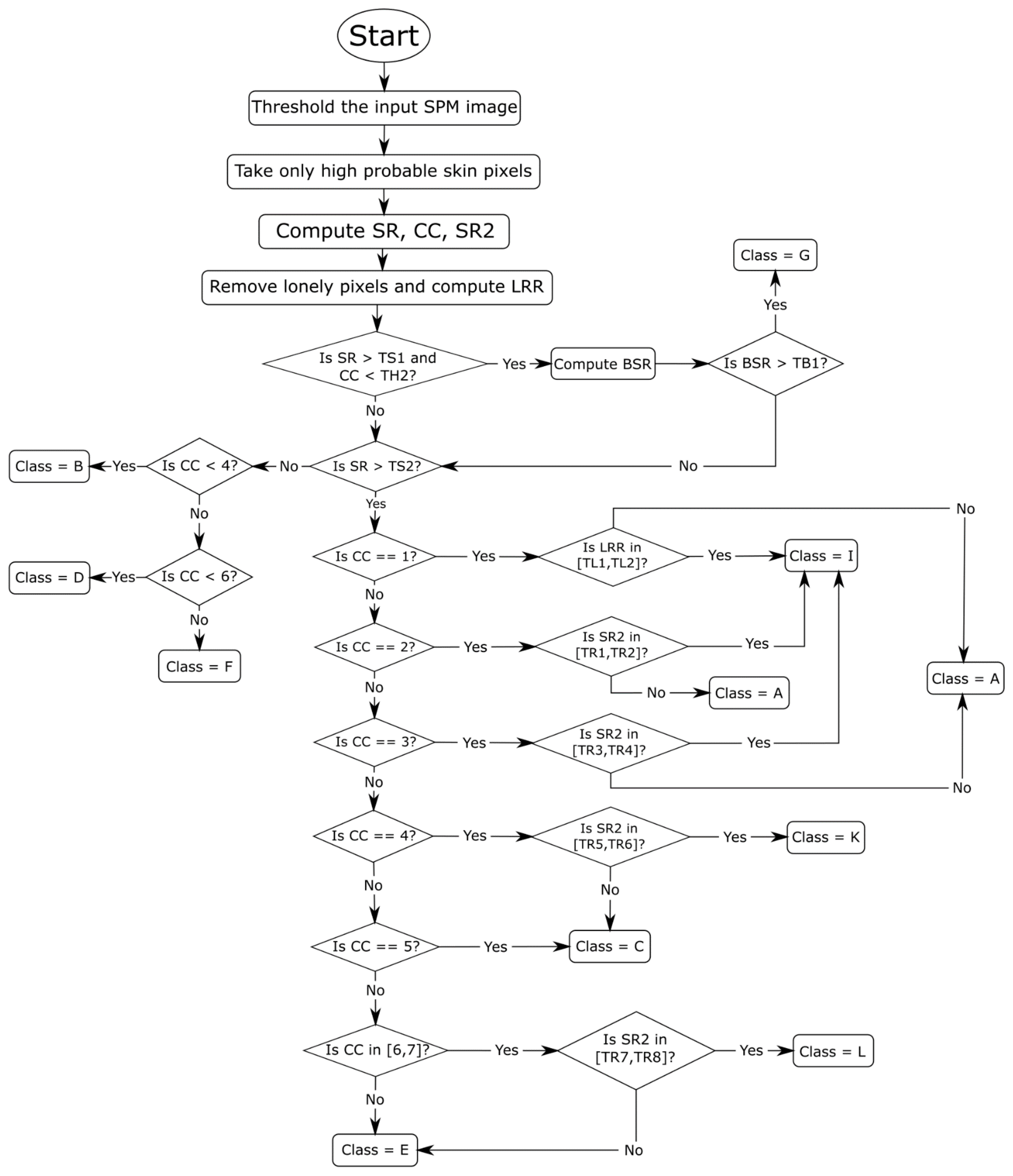
In this paper, we expanded the approach taken in reference [21] for refining the segmentation results of a CNN applied to skin detection, an approach that is based on learning to identify classes of images that will then govern the selection of the morphological postprocessing method. Unlike the method proposed in reference [21], the detected classes in this work determine two types of postprocessing techniques: a set of morphological functions and a homogeneity function. As was the case in reference [21], the classes were determined by a visual inspection of images. After that, a learning procedure was designed to automatically classify each image into one of several classes according to the flow chart in Figure 1.
As mentioned in the introduction, five such classes were originally identified in reference [21]; in this work, a postprocessing method was chosen (see Table 1) based on one of the following eleven classes:
- Class A: images in which there is a very near foreground that implies a high percentage of skin pixels and few connected components.
- Class B: images in which there is only the face of the person that is not too close to the camera.
- Class C: images where there is a single person with body parts showing, e.g., the face, arms, and legs, on separated connected components.
- Class D: images in which there is only one person far from the camera.
- Class E: images in which there is a group of people and no connected component that prevails over the others.
- Class F: images in which there is the presence of a far group of people, which implies an elevated number of connected components and a few skin pixels with respect to the total number of image pixels.
- Class G: images in which the background is erroneously classified as skin pixels.
- Class H: images without skin.
- Class I: images in which the foreground is very close, and the largest connected component takes almost all the skin pixels.
- Class K: images in which there is a single person and a connected component that, regarding dimensions, overcome the others.
- Class L: images in which there is a small group of people and a connected component that triumphs over the others.
After the class assignment, the selected postprocessing method was applied to create the final mask.
Compared to the classes identified in reference [21], classes B–D are expanded into several categories. Classes C and D, originally having to do with groups, are further broken down here into classes E, F, and L, and class B (originally called “Face in foreground”) is generalized here into classes D and K to include all the body parts. Moreover, the notion of the foreground is further expanded into classes A, B, and I to distinguish different foreground situations. It should also be pointed out that the only difference between classes A, B, and C and classes I, K, and L in Table 1 is the type of postprocessing method applied in the final step.
A CNN applied to skin detection provides an image called the Skin Probability Map (SPM), which corresponds to the classifier score at the pixel level, i.e., the probability of each pixel to be labeled as skin. This probability was rescaled to the range [0, 255] and taken as the input of our postprocessing method. Binary classification was performed on every pixel to the classes skin/nonskin based on the postprocessing function. The SPM was passed into a threshold algorithm based on Otsu’s method [34], where an optimal threshold was selected by the discriminant criterion. In this case, the pixels were classified as belonging to one of three sets: a high, discrete, or low probability of being a skin pixel, depending on the pixel’s value. Only pixels belonging to the first set were considered true skin.
In reference [21], three features (items 1–3 below) were computed to assign the image to the right class. The method proposed here includes two additional features (items 4 and 5):
- (1)
- Skin Ratio (SR) [2]: the percentage of skin pixels in the image;
- (2)
- Connected Components (CC) [2]: the number of skin regions;
- (3)
- Border Skin Ratio (BSR) [2]: a measurement reflecting the amount of skin surface recognized within a 1-pixel frame as a border. It is the ratio between the numbers of pixels of skin detected on the top, right, and left sides (excluding the bottom) of the image over the total number of pixels in those sides;
- (4)
- SR2: similar to SR, except that the ratio between the largest skin region area and the number of skin pixels is computed;
- (5)
- Largest Region Ratio (LRR): the ratio between the largest region area and the image dimension; LRR is useful only when the image has a foreground that is near. After computing this value, all skin regions composed of only one pixel are removed.
Depending on the assumed values of these features, the image is assigned to one of the eleven possible classes, as shown in Figure 1 and in the pseudocode below.
There are four possible postprocessing methods, three based on different sets of morphological operators, such as multiplication and dilatation, and one on homogeneity [3], a region-based algorithm. The homogeneity approach checks the pixel and its neighborhood before classifying it in the following way:
- (1)
- The SPM image is normalized; and, only in the first loop, a threshold T is set to 0.2, so that if a pixel has a value greater than T it will be labeled as skin;
- (2)
- Regions with an area less than 300 pixels are removed;
- (3)
- Every region is evaluated to decide whether it can be homogenous or not using this formula:
It has been demonstrated that the homogeneity method works well when people are near [3]. Therefore, the values of CC, SR2, and LRR are used to select the appropriate images to be processed by this algorithm (Algorithm 1).
The other postprocessing functions are based on the five morphological operators (see Table 2) used in reference [21] but which are combined here in three sequences (see Table 3).
| Algorithm 1 Pseudocode of the learned postprocessing method. |
|
1: postP(spm) 2: class ← H 3: img ← threshold(spm) 4: compute SR, CC, SR2 on img 5: imgO2 ← remove lonely pixels 6: compute LRR on imgO2 7: if SR > TS1 & CC < 6 8: compute BSR on img 9: if BSR > TB1 10: class ← G 11: if (SR > TS2) & (class NOT G) 12: if CC == 1 13: if LRR in [TL1, TL2] 14: class ← I 15: else 16: class ← A 17: if CC == 2 18: if SR2 in [TR1, TR2] 19: class ← I 20: else 21: class ← A 22: if CC == 3 23: if SR2 in [TR3, TR4] 24: class ← I 25: else 26: class ← A 27: if CC == 4 28: if SR2 in [TR5, TR6] 29: class ← K 30: else 31: class ← C 32: if CC == 5 33: class ← C 34: if CC in [6,7] 35: if SR2 in [TR7, TR8] 36: class ← L 37: else 38: class ← E 49: else 40: class ← E 41: if (SR < TS3) & (class NOT G) 42: if CC < 4 43: class ← B 44: if CC < 6 45: class ← D 46: else 47: class ← F 48: switch class 49: case I, K, L 50: mask ← homogeneity(img) 51: case A, B, C, E 52: mask ← morphological_set#1 53: case D, F 54: mask ← morphological_set#2 55: case G 56: mask ← morphological_set#3 57: return mask |
The value of all the thresholds (see Table 4) used in the algorithm above are learned from the training set of the ECU dataset.
3. Experimental Results
Making fair comparisons between the skin detection algorithms and datasets is problematic, because many datasets are created by different research groups, have unreliable ground truths (mislabeled sections), and are intended for many separate applications. For fair comparisons, the authors of reference [13] proposed a framework for skin detector comparisons that is based on how well new algorithms perform across the following ten datasets:
- (1)
- ECU [36]: a dataset that contains 4000 color images. The dataset is divided into two, with the first half making up the training set;
- (2)
- Compaq [37]: a widely used skin dataset that contains 4675 images;
- (3)
- UChile [38]: a challenging, though relatively small dataset, that includes 103 images with complex backgrounds and different illumination conditions;
- (4)
- Schmugge [39]: 845 images extracted from several face datasets;
- (5)
- Feeval [40]: a dataset containing 8991 frames that were taken from twenty-five videos of low-quality found online. The performance is the average result considering all the frames for a given video; in other words, each video is viewed as one image when it comes to reporting the performance;
- (6)
- MCG [39]: a dataset containing 1000 images;
- (7)
- VMD [41]: a dataset that includes 285 images collected from a number of different datasets that are publicly available for human action recognition;
- (8)
- SFA [42]: a dataset that contains 3354 skin samples and 5590 nonskin samples extracted from two popular face recognition datasets: the FERET database and the AR Face Database;
- (9)
- Pratheepan [43]: a dataset with only 78 images;
- (10)
- HGR [44]: a dataset intended to evaluate gesture recognition. In this dataset, the image sizes are large. For this reason, the images in HGR2A (85 images) and in HGR2B (574 images) were reduced by 0.3.
For a more extensive description of the ten datasets, see reference [13].
Since skin detection is a binary problem, all standard measures of performance evaluation (accuracy, precision, recall, Kapp, , and the ROC curve) are appropriate. is the most common performance indicator used in the literature, however. For this reason, this indicator is the one recommended by the authors of reference [13] and is defined as
where , are false negatives, are true positives, and are false positives. When used as the performance measure in skin detection, is averaged at the pixel level rather than at the image level. This way of averaging is independent of variations in the sizes of images, which are different for each dataset.
The first set of experiments, reported in Table 5 compares the performance for the skin detector DeepLabV3+ and FusAct3 with three different postprocessing methods:
The Wilcoxon signed-rank test shows that the postprocessing approach proposed here coupled with DeepLabV3+ outperforms all the other methods based on DeepLabV3+ (including OR) with a p-value of 0.0001; when coupled with FusAct3, the new postprocessing approach outperforms the other methods based on FusAct3 (including OR) with a p-value of 0.1. For both DeepLabV3+ and FusAct3 (see the discussion in Section 2.1), there was no statistical difference between them using OR, MorphBASE, and LearnMorph.
Comparing the stand-alone approaches in Table 5 and the Wilcoxon signed-rank tests, the following can be concluded:
- The quality of the images has an impact on the performance; thus, the performance diverges considerably between datasets.
- When it comes to deep learning, fine-tuning on each dataset is critical. Take, for example, the HGR dataset created for the task of gesture recognition; certainly, segmentation by a CNN specifically trained for this task would produce better results, but obtaining the best performance on a particular dataset is not the aim here. For fair comparisons across all datasets representing different tasks, the same configuration has to be maintained.
- The new postprocessing method improves the performance of the base methods in nearly all the other datasets. This is of particular interest, given that FusAct3 obtains a state-of-the-art performance.
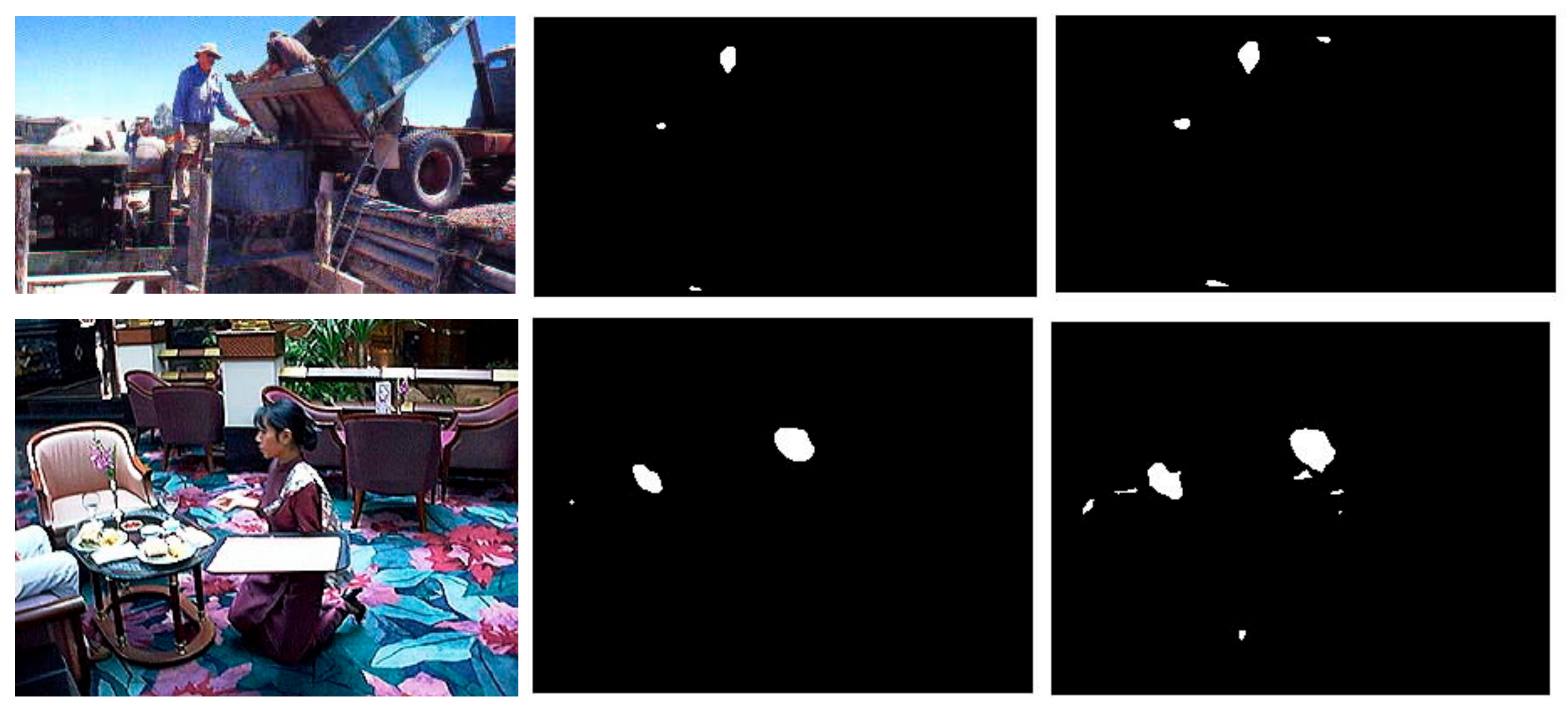
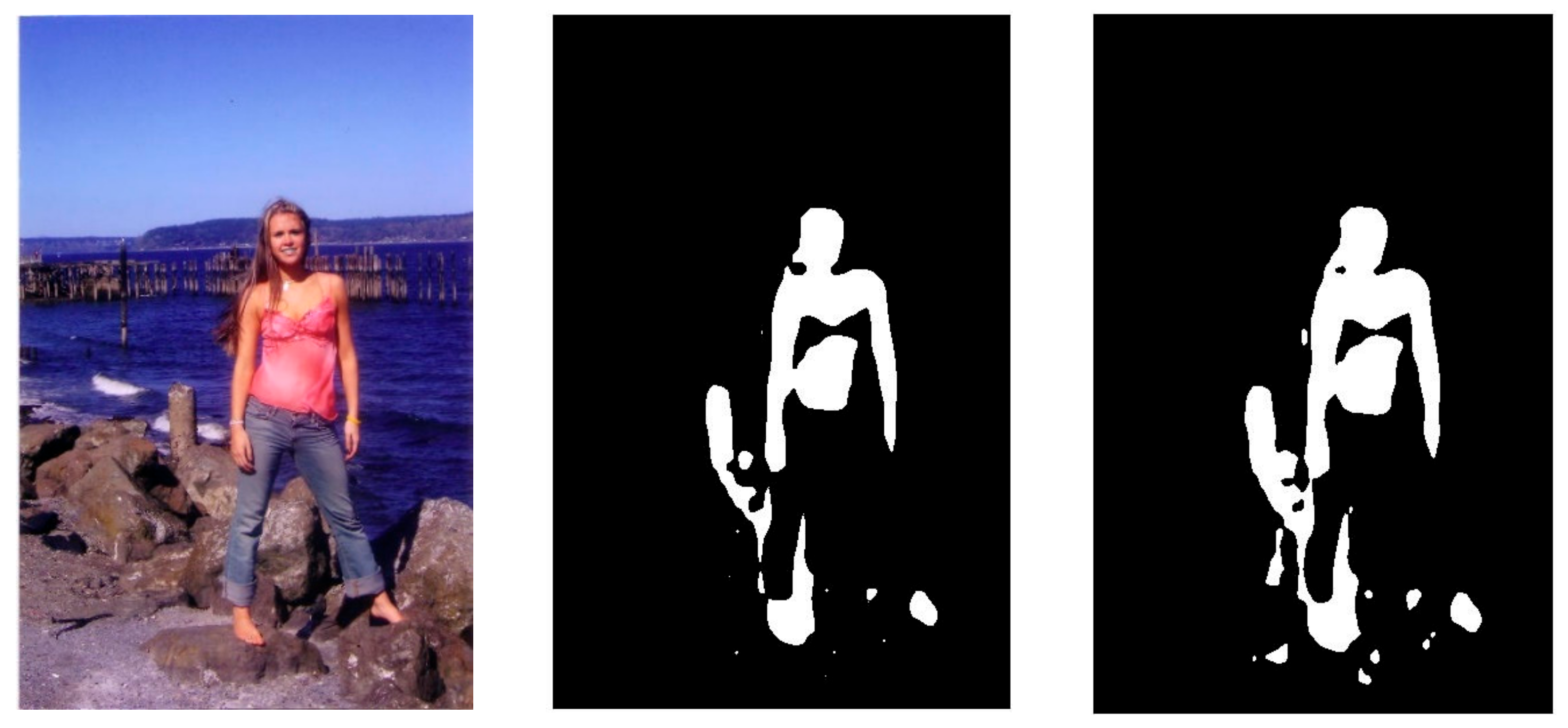
Visually examining some of the postprocessing images obtained by the refinement of our new method MorphHom would provide insight into why the performance is improved using it. In Figure 2, three such images are provided with and without the addition of MorphHom.
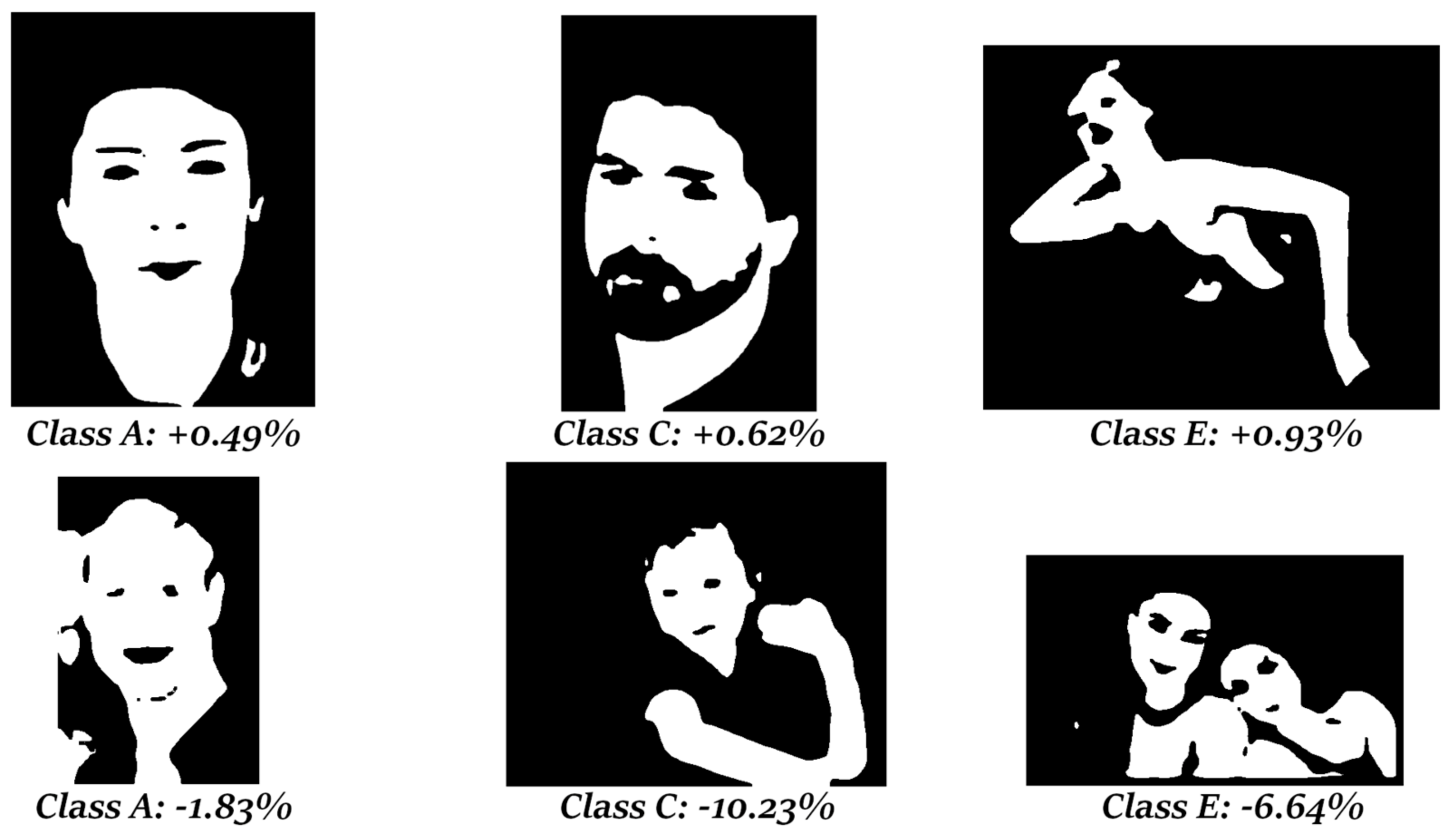
As noted in the introduction, the main aim of this work compared to [21] is to find a criterion for selecting images in need of a homogeneity postprocessing method instead of a morphological approach. Given the results produced above, it is clear that the homogeneity algorithm improves the final segmentation when there is a connected component that prevails over the others. Some examples and the relative increment/decrement in performance after applying the homogeneity are shown in the following masks (Figure 3).
4. Conclusions
A new post-processing method for enhancing the classification of skin detectors was presented in this work that assigns a class to an image and then applies either a series of morphological operators or a homogeneity function to generate the final mask. Eleven classes of images were specified, and the postprocessing method was selected based on the class to which the image belongs. Experimentation across ten datasets representative of several problem domains demonstrated that the application of this approach for learning to select the best postprocessing method from this set of postprocessing possibilities significantly improved the performance of the base skin detectors.
Further studies are planned that will investigate the best postprocessing techniques for low-quality images, since these images failed to perform well with DeepLabV3+. This degradation in performance with low-quality images was probably the consequence of training the deep network on high-quality images only. One way to tackle this problem is to retrain the CNN by applying different types of data augmentation that produce low-quality images and then test whether this improves the segmentation performance on these types of images.
Another interesting topic is the application of morphological operators in the segmentation process. Recently, a few studies [22,23,45] have emerged based on the definition of a new topology of networks, including morphological operators. These semi-hybrid versions of traditional convolution and pseudo-morphological operations could be adapted to the segmentation problem with the aim of substituting the handcrafted postprocessing step. Additional studies should also be conducted to handle the skin segmentation of people of different races using a dataset developed for this purpose, such as that in presented in reference [14], which should be available to the public shortly.
Author Contributions
L.N. and D.B. conceived the presented idea. L.N. performed the experiments. S.B., A.L., L.N., and D.B. wrote the manuscript. A.L. and S.B. provided some resources. All authors have read and agreed to the published version of the manuscript.
Funding
This research received no external funding.
Institutional Review Board Statement
Not applicable.
Informed Consent Statement
Not applicable.
Data Availability Statement
All ten datasets are either publicly available or available upon request by the authors of the papers cited for each dataset. All MATLAB source code is available at https://github.com/LorisNanni/Postprocessing-for-Skin-Detection.
Acknowledgments
We acknowledge the support of NVIDIA’s GPU Grant Program that a TitanX GPU for training the deep learner in this work.
Conflicts of Interest
The authors declare no conflict of interest.
References
- Chyad, M.A.; Alsattar, H.A.; Zaidan, B.B.; Zaidan, A.A.; Al Shafeey, G.A. The landscape of research on skin detectors: Coherent taxonomy, open challenges, motivations, recommendations and statistical analysis, future directions. IEEE Access 2019, 7, 106536–106575. [Google Scholar] [CrossRef]
- Naji, S.; Jalab, H.A.; Kareem, S.A. A survey on skin detection in colored images. Artif. Intell. Rev. 2018, 52, 1041–1087. [Google Scholar] [CrossRef]
- Kakumanu, P.; Makrogiannis, S.; Bourbakis, N. A survey of skin-color modeling and detection methods. Pattern Recognit. 2007, 40, 1106–1122. [Google Scholar] [CrossRef]
- Asari, V.K.; Seow, M.; Valaparla, D. Neural Network Based Skin Color Model for Face Detection. In Proceedings of the 2013 IEEE Applied Imagery Pattern Recognition Workshop (AIPR), Washington, DC, USA, 23–25 October 2003; p. 141. [Google Scholar]
- Khan, R.; Hanbury, A.; Stöttinger, J. Skin Detection: A Random Forest Approach. In Proceedings of the 2010 IEEE International Conference on Image Processing, Hong Kong, China, 26–29 September 2010; pp. 4613–4616. [Google Scholar]
- Sebe, N.; Cohen, I.; Huang, T.; Gevers, T. Skin Detection: A Bayesian Network Approach. In Proceedings of the 17th International Conference on Pattern Recognition, Cambridge, UK, 26 August 2004; pp. 903–906. [Google Scholar]
- Chakraborty, B.K.; Bhuyan, M.K. Image specific discriminative feature extraction for skin segmentation. Multimed. Tools Appl. 2020, 79, 18981–19004. [Google Scholar] [CrossRef]
- Poudel, R.P.; Zhang, J.J.; Liu, D.; Nait-Charif, H. Skin color detection using region-based approach. Int. J. Image Process. (IJIP) 2013, 7, 385. [Google Scholar]
- Chen, W.-C.; Wang, M.-S. Region-based and content adaptive skin detection in color images. Int. J. Pattern Recognit. Artif. Intell. 2007, 21, 831–853. [Google Scholar] [CrossRef]
- Xu, T.; Zhang, Z.; Wang, Y. Patch-wise skin segmentation of human body parts via deep neural networks. J. Electron. Imaging 2015, 24, 43009. [Google Scholar] [CrossRef]
- Zuo, H.; Fan, H.; Blasch, E.; Ling, H. Combining convolutional and recurrent neural networks for human skin detection. IEEE Signal Process. Lett. 2017, 24, 289–293. [Google Scholar] [CrossRef]
- Kim, Y.; Hwang, I.; Cho, N.I. Convolutional Neural Networks and Training Strategies for Skin Detection. In Proceedings of the 2017 IEEE International Conference on Image Processing (ICIP), Beijing, China, 17–20 September 2017; pp. 3919–3923. [Google Scholar]
- Lumini, A.; Nanni, L. Fair comparison of skin detection approaches on publicly available datasets. Expert Syst. Appl. 2020, 160, 113677. [Google Scholar] [CrossRef]
- Arsalan, M.; Kim, D.S.; Owais, M.; Park, K.R. OR-Skip-Net: Outer residual skip network for skin segmentation in non-ideal situations. Expert Syst. Appl. 2020, 141, 112922. [Google Scholar] [CrossRef]
- Tarasiewicz, T.; Nalepa, J.; Kawulok, M. Skinny: A Lightweight U-net for Skin Detection and Segmentation. In Proceedings of the 2020 IEEE International Conference on Image Processing (ICIP), Abu Dhabi, United Arab Emirates, 25–28 October 2020; pp. 2386–2390. [Google Scholar]
- Paracchini, M.; Marcon, M.; Villa, F.; Tubaro, S. Deep skin detection on low resolution grayscale images. Pattern Recognit. Lett. 2020, 131, 322–328. [Google Scholar] [CrossRef]
- Dourado, A.; Guth, F.; de Campos, T.E.; Weigang, L. Domain adaptation for holistic skin detection. arXiv 2020, arXiv:1903.06969. Available online: https://arxiv.org/abs/1903.06969 (accessed on 30 May 2021).
- Ma, C.-H.; Shih, H.-C. Human Skin Segmentation Using Fully Convolutional Neural Networks. In Proceedings of the 2018 IEEE 7th Global Conference on Consumer Electronics (GCCE), Nara, Japan, 9–12 October 2018; pp. 168–170. [Google Scholar]
- Yong-Jia, Z.; Shu-Ling, D.; Xiao, X. A Mumford-Shah Level-Set Approach for Skin Segmentation Using a New Color Space. In Proceedings of the 2008 Asia Simulation Conference—7th International Conference on System Simulation and Scientific Computing, Beijing, China, 10–12 October 2008; pp. 307–310. [Google Scholar]
- Kawulok, M. Energy-based blob analysis for improving precision of skin segmentation. Multimed. Tools Appl. 2010, 49, 463–481. [Google Scholar] [CrossRef]
- Lumini, A.; Nanni, L.; Codogno, A.; Berno, F. Learning morphological operators for skin detection. J. Artif. Intell. Syst. 2019, 1, 60–76. [Google Scholar] [CrossRef] [Green Version]
- Franchi, G.; Fehri, A.; Yao, A. Deep morphological networks. Pattern Recognit. 2020, 102, 107246. [Google Scholar] [CrossRef]
- Nogueira, K.; Chanussot, J.; Mura, M.D.; Schwartz, W.R.; dos Santos, J.A. An introduction to deep morphological networks. arXiv 2019, arXiv:1906.01751. Available online: https://arxiv.org/abs/1906.01751 (accessed on 30 May 2021).
- Song, W.; Zheng, N.; Zheng, R.; Zhao, X.B.; Wang, A. Digital image semantic segmentation algorithms: A survey. J. Inf. Hiding Multimed. Signal Process. 2019, 10, 196–211. [Google Scholar]
- Long, J.; Shelhamer, E.; Darrell, T. Fully Convolutional Networks for Semantic Segmentation. In Proceedings of the IEEE Conference on Computer Vision and Pattern Recognition, Boston, MA, USA, 7–12 June 2015; pp. 3431–3440. [Google Scholar]
- Badrinarayanan, V.; Kendall, A.; Cipolla, R. SegNet: A deep convolutional encoder-decoder architecture for image segmenta-tion. IEEE Trans. Pattern Anal. Mach. Intell. 2017, 39, 2481–2495. [Google Scholar] [CrossRef]
- Simonyan, K.; Zisserman, A. Very deep convolutional networks for large-scale image recognition. arXiv 2014, arXiv:1409.1556. Available online: https://arxiv.org/abs/1409.1556 (accessed on 30 May 2021).
- Ronneberger, O.; Fischer, P.; Brox, T. U-net: Convolutional Networks for Biomedical Image Segmentation. In Proceedings of the International Conference on Medical Image Computing and Computer-Assisted Intervention, Munich, Germany, 5–9 October 2015; pp. 234–241. [Google Scholar]
- Nanni, L.; Lumini, A.; Ghidoni, S.; Maguolo, G. Stochastic selection of activation layers for convolutional neural networks. Sensors 2020, 20, 1626. [Google Scholar] [CrossRef] [PubMed] [Green Version]
- Chen, L.-C.; Zhu, Y.; Papandreou, G.; Schroff, F.; Adam, H. Encoder-Decoder with Atrous Separable Convolution for Semantic Image Segmentation. In Proceedings of the European Conference on Computer Vision—ECCV 2018, Munich, Germany, 8–14 September 2018. [Google Scholar]
- Chen, L.-C.; Papandreou, G.; Schroff, F.; Adam, H. Rethinking atrous convolution for semantic image segmentation. arXiv 2017, arXiv:1706.05587. Available online: https://arxiv.org/abs/1706.05587 (accessed on 30 May 2021).
- Holschneider, M.; Kronland-Martinet, R.; Morlet, J.; Tchamitchian, P. A real-time algorithm for signal analysis with the help of the wavelet transform. In Wavelets Time-Frequency Methods and Phase Space; Springer: Berlin/Heidelberg, Germany, 1989. [Google Scholar]
- Maguolo, G.; Nanni, L.; Ghidoni, S. Ensemble of convolutional neural networks trained with different activation functions. Expert Syst. Appl. 2021, 166, 114048. [Google Scholar] [CrossRef]
- Otsu, N. A threshold selection method from gray-level histograms. IEEE Trans. Syst. Man Cybern. 1979, 9, 62–66. [Google Scholar] [CrossRef] [Green Version]
- Gonzalez, R.C.; Woods, R.E. Digital Image Processing, 2nd ed.; Addison-Wesley Longman Publishing Co., Inc.: Boston, MA, USA, 2001. [Google Scholar]
- Phung, S.; Bouzerdoum, A.; Chai, D. Skin segmentation using color pixel classification: Analysis and comparison. IEEE Trans. Pattern Anal. Mach. Intell. 2005, 27, 148–154. [Google Scholar] [CrossRef] [Green Version]
- Jones, M.; Rehg, J. Statistical Color Models with Application to Skin Detection. In Proceedings of the 1999 IEEE Computer Society Conference on Computer Vision and Pattern Recognition, Fort Collins, CO, USA, 23–25 June 1999. [Google Scholar]
- Ruiz-Del-Solar, J.; Verschae, R. Skin Detection Using Neighborhood Information. In Proceedings of the Sixth IEEE International Conference on Automatic Face and Gesture Recognition, Seoul, Korea, 19 May 2004; pp. 463–468. [Google Scholar]
- Schmugge, S.J.; Jayaram, S.; Shin, M.C.; Tsap, L.V. Objective evaluation of approaches of skin detection using ROC analysis. Comput. Vis. Image Underst. 2007, 108, 41–51. [Google Scholar] [CrossRef]
- Stöttinger, J.; Hanbury, A.; Liensberger, C.; Khan, R. Skin Paths for Contextual Flagging Adult Videos. In Proceedings of the International Symposium on Visual Computing, Las Vegas, NV, USA, 30 November–2 December 2009. [Google Scholar]
- SanMiguel, J.C.; Suja, S. Skin detection by dual maximization of detectors agreement for video monitoring. Pattern Recognit. Lett. 2013, 34, 2102–2109. [Google Scholar] [CrossRef] [Green Version]
- Casati, J.P.B.; Moraes, D.R.; Rrodrigues, E.L.L. SFA: A Human Skin Image Database Based on FERET and AR Facial Images. In Proceedings of the IX Workshop de Visão Computacional, Anais do VIII Workshop de Visão Computacional, Rio de Janeiro, Brazil, 3–5 June 2013. [Google Scholar]
- Tan, W.R.; Chan, C.S.; Yogarajah, P.; Condell, J. A fusion approach for efficient human skin detection. IEEE Trans. Ind. Inform. 2011, 8, 138–147. [Google Scholar] [CrossRef] [Green Version]
- Kawulok, M.; Kawulok, J.; Nalepa, J.; Smolka, B. Self-adaptive algorithm for segmenting skin regions. EURASIP J. Adv. Signal Process. 2014, 2014, 1–22. [Google Scholar] [CrossRef] [Green Version]
- Mellouli, D.; Hamdani, T.M.; Sanchez-Medina, J.J.; Ben Ayed, M.; Alimi, A.M. Morphological convolutional neural network architecture for digit recognition. IEEE Trans. Neural Netw. Learn. Syst. 2019, 30, 2876–2885. [Google Scholar] [CrossRef]
Figure 1.
Flow chart of the image classification approach.

Figure 2.
RGB image (left), skin mask via FusAct3 + MorphHom (middle), and skin mask via FusAct3 (right). Sample images in column 1 were taken from the publicly available ECU dataset located at https://documents.uow.edu.au/~phung/download.html, (accessed on 31 May 2021).
Figure 2.
RGB image (left), skin mask via FusAct3 + MorphHom (middle), and skin mask via FusAct3 (right). Sample images in column 1 were taken from the publicly available ECU dataset located at https://documents.uow.edu.au/~phung/download.html, (accessed on 31 May 2021).


Figure 3.
First row: images from the classes (A, C, and E) in which the homogeneity method obtained better results and the relative increment over the F1-measure. Second row: pictures from the same classes in which the homogeneity algorithm gave poor results with respect to the morphological approach.


Table 1.
Image classification classes and the related postprocessing methods.
| Class | Short Description | Postprocessing |
|---|---|---|
| A | Foreground near | Morphological (Set#1) |
| B | Foreground far | Morphological (Set#1) |
| C | With body parts near | Morphological (Set#1) |
| D | With body parts far | Morphological (Set#2) |
| E | Group near | Morphological (Set#1) |
| F | Group far | Morphological (Set#2) |
| G | Background considered as skin | Morphological (Set#3) |
| H | No skin | - |
| I | Foreground near | homogeneity |
| K | With body parts near | homogeneity |
| L | Group near | homogeneity |
Table 2.
Morphological MATLAB operators. Note that the parameters I and J are masks, SE is the structuring element and P is a pixel count value.
Table 2.
Morphological MATLAB operators. Note that the parameters I and J are masks, SE is the structuring element and P is a pixel count value.
| Morphological Operators | Description |
|---|---|
| imerode(I, SE) | Erosion |
| imdilate(I, SE) | Dilation |
| imfill(I, ‘holes’) | Mask-filling ‘holes’ |
| immultiply(I, J) | Pixel-by-pixel multiplication of the two masks |
| bwareaopen(I, P) | Area removal from the mask with pixel count < P |
Table 3.
Morphological operations (listed as MATLAB commands [35]) performed on each class, except H (no skin). Note: although the first two rows use the same set of operators, the disks employed as structuring elements have different sizes.
Table 3.
Morphological operations (listed as MATLAB commands [35]) performed on each class, except H (no skin). Note: although the first two rows use the same set of operators, the disks employed as structuring elements have different sizes.
| Class | Morphological Set |
|---|---|
| A, B, C, E | (Set#1) = imerode→bwareaopen→imdilate→immultiply |
| D, F | (Set#2) = imerode→bwareaopen→imdilate→immultiply |
| G | (Set#3) = imerode→immultiply→imfill |
Table 4.
Thresholds used in the pseudocode.
| TS1 = 0.12 | TS2 = 0.1685 | TS3 = 0.1685 | TB1 = 1 | TL1 = 3.5e-6 | TL2 = 86.3e-6 | TR1 = 0.9967 |
| TR2 = 0.9995 | TR3 = 0.9730 | TR4 = 0.9992 | TR5 = 0.9701 | TR6 = 0.9979 | TR7 = 0.8736 | TR8 = 0.9984 |
Table 5.
F1-measure of the tested methods (N.B. bold-face indicates superior results).
| Method | DataSet | Avg | |||||||||||
|---|---|---|---|---|---|---|---|---|---|---|---|---|---|
| FV | Prat | MCG | UC | CMQ | SFA | HGR | Sch | VMD | ECU | VT | |||
| DeepLabV3+ | OR | 0.759 | 0.831 | 0.872 | 0.881 | 0.799 | 0.946 | 0.950 | 0.763 | 0.592 | 0.917 | 0.679 | 0.817 |
| MorphBASE | 0.763 | 0.835 | 0.874 | 0.882 | 0.803 | 0.946 | 0.951 | 0.765 | 0.583 | 0.918 | 0.679 | 0.818 | |
| LearnMorph | 0.762 | 0.835 | 0.874 | 0.882 | 0.788 | 0.946 | 0.951 | 0.766 | 0.583 | 0.918 | 0.679 | 0.817 | |
| MorphHom | 0.765 | 0.852 | 0.877 | 0.888 | 0.813 | 0.947 | 0.957 | 0.773 | 0.622 | 0.926 | 0.691 | 0.828 | |
| FusAct3 | OR | 0.792 | 0.854 | 0.881 | 0.886 | 0.817 | 0.952 | 0.959 | 0.771 | 0.661 | 0.926 | 0.710 | 0.837 |
| MorphBASE | 0.794 | 0.856 | 0.882 | 0.885 | 0.819 | 0.952 | 0.959 | 0.771 | 0.636 | 0.927 | 0.710 | 0.836 | |
| LearnMorph | 0.794 | 0.856 | 0.882 | 0.885 | 0.807 | 0.953 | 0.959 | 0.771 | 0.636 | 0.927 | 0.710 | 0.835 | |
| MorphHom | 0.782 | 0.874 | 0.882 | 0.885 | 0.828 | 0.952 | 0.963 | 0.774 | 0.669 | 0.935 | 0.717 | 0.842 | |
Publisher’s Note: MDPI stays neutral with regard to jurisdictional claims in published maps and institutional affiliations. |
© 2021 by the authors. Licensee MDPI, Basel, Switzerland. This article is an open access article distributed under the terms and conditions of the Creative Commons Attribution (CC BY) license (https://creativecommons.org/licenses/by/4.0/).
Share and Cite
MDPI and ACS Style
Baldissera, D.; Nanni, L.; Brahnam, S.; Lumini, A. Postprocessing for Skin Detection. J. Imaging 2021, 7, 95. https://0-doi-org.brum.beds.ac.uk/10.3390/jimaging7060095
AMA Style
Baldissera D, Nanni L, Brahnam S, Lumini A. Postprocessing for Skin Detection. Journal of Imaging. 2021; 7(6):95. https://0-doi-org.brum.beds.ac.uk/10.3390/jimaging7060095
Chicago/Turabian StyleBaldissera, Diego, Loris Nanni, Sheryl Brahnam, and Alessandra Lumini. 2021. "Postprocessing for Skin Detection" Journal of Imaging 7, no. 6: 95. https://0-doi-org.brum.beds.ac.uk/10.3390/jimaging7060095
Note that from the first issue of 2016, this journal uses article numbers instead of page numbers. See further details here.