
Restoration and Enhancement of Historical Stereo Photos †


1
Department of Information Engineering, Università degli Studi di Firenze, 50139 Firenze, Italy
2
Department of Math and Computer Science, Università degli Studi di Palermo, 90123 Palermo, Italy
*
Author to whom correspondence should be addressed.
†
This paper is an extended version of our paper published in The 25th International Conference on Pattern Recognition Workshop (ICPRW 2020) on Fine Art Pattern Extraction and Recognition (FAPER 2020), Online, 10–15 January 2021.
J. Imaging 2021, 7(7), 103; https://0-doi-org.brum.beds.ac.uk/10.3390/jimaging7070103
Submission received: 20 April 2021
/
Revised: 11 June 2021
/
Accepted: 21 June 2021
/
Published: 24 June 2021
(This article belongs to the Special Issue Fine Art Pattern Extraction and Recognition)
Abstract
:Restoration of digital visual media acquired from repositories of historical photographic and cinematographic material is of key importance for the preservation, study and transmission of the legacy of past cultures to the coming generations. In this paper, a fully automatic approach to the digital restoration of historical stereo photographs is proposed, referred to as Stacked Median Restoration plus (SMR+). The approach exploits the content redundancy in stereo pairs for detecting and fixing scratches, dust, dirt spots and many other defects in the original images, as well as improving contrast and illumination. This is done by estimating the optical flow between the images, and using it to register one view onto the other both geometrically and photometrically. Restoration is then accomplished in three steps: (1) image fusion according to the stacked median operator, (2) low-resolution detail enhancement by guided supersampling, and (3) iterative visual consistency checking and refinement. Each step implements an original algorithm specifically designed for this work. The restored image is fully consistent with the original content, thus improving over the methods based on image hallucination. Comparative results on three different datasets of historical stereograms show the effectiveness of the proposed approach, and its superiority over single-image denoising and super-resolution methods. Results also show that the performance of the state-of-the-art single-image deep restoration network Bringing Old Photo Back to Life (BOPBtL) can be strongly improved when the input image is pre-processed by SMR+.
1. Introduction
Photographic material of the XIX and XX centuries is an invaluable source of information for historians of art, architecture and sociology, as it allows them to track the changes occurred over the decades to a community and its living environment. Unfortunately, due to the effect of time and bad preservation conditions, most of the survived photographic heritage is partially damaged, and needs restoration, both at the physical (cardboard support, glass negatives, films, etc.) and digital (the image content acquired through scanners) levels. Dirt, scratches, discoloration and other signs of aging strongly reduce the visual quality of photos [1]. A similar situation also holds for the cinematographic material [2].
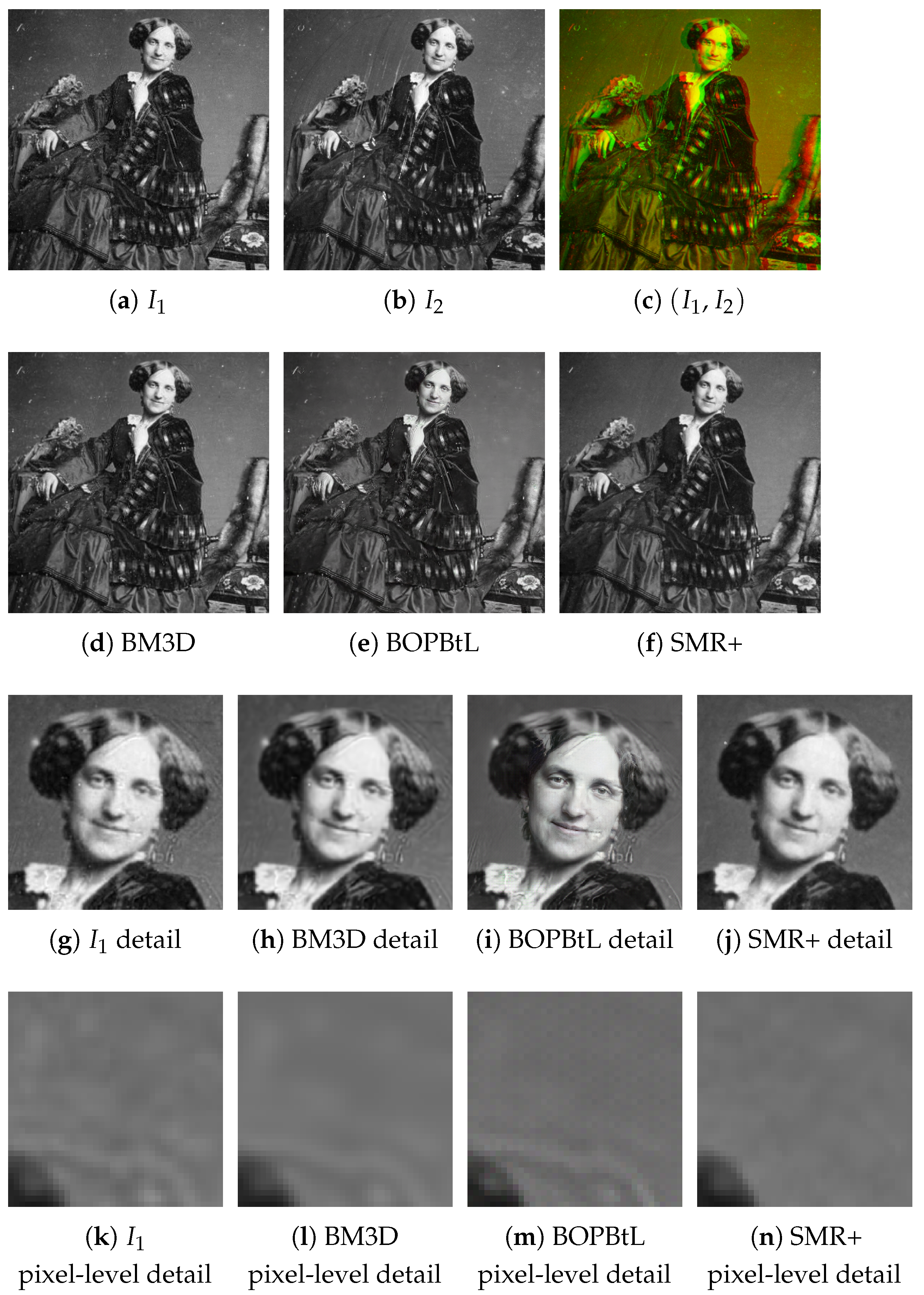
Digital restoration of both still images and videos has attracted considerable interest from the research community in the early 2000s. This has led to the development of several tools that improve the visual quality. Some approaches rely on the instantiation of noise models, which can either be fixed a priori or derived from the input images [3,4,5]. Other approaches detect damaged areas of the image and correct them according to inpainting techniques [6]. Self-correlation inside the image, or across different frames in videos, is often exploited in this context, under the assumption that zero-mean additive noise cancels out as the available number of image data samples increases [7,8,9]. A similar idea is exploited by super-resolution techniques that enhance image quality by pixel interpolation [10,11]. In recent years, the algorithmic methods above have been sided by methods based on deep learning that can infer the image formation model or the scene content [12] from a training set in order to inject this information into the final output, a process called image hallucination [13,14,15]. Although the final image may often alter the original image data content, and hence cannot be fully trusted (e.g., in the medical diagnosis domain), the hallucination methods can give visually pleasing results (see Figure 1).
Stereoscopy has accompanied photography since its very birth in the nineteenth century, with ups and downs in popularity through time. Notwithstanding the lesser spread of stereo photography with respect to standard (monocular) photography, many digital archives with thousands of stereo images exist, some of which are freely available on the web. Stereo photos have a richer content than standard ones, as they present two different views of the same scene, thus explicitly introducing content redundancy and implicitly embedding information about scene depth. This characteristic can be exploited also in digital noise removal, enhancement and restoration, since a damaged area in one image can be reconstructed from the other image, provided that the correspondences between the two images are known. At a first glance, the above-mentioned approach looks similar to that of video restoration from multiple video frames, in which the scene is acquired in subsequent time instants from slightly changed viewpoints. However, stereo images have their own peculiarities, and actually introduce in the restoration process more complications than video frames, which in movies typically exhibit an almost static and undeformed background, differently from stereo pairs. As a matter of fact, although several advances have been recently made in stereo matching and dense optical flow estimation [16], the problem is hard and far from being fully solved, especially in the case of very noisy and altered images such as those generated by early photographic stereo material. To the best of the authors’ knowledge, stereo photo characteristics have been employed only for the super-resolution enhancement or deblurring of modern, clean photos [17,18,19]. On the other hand, the image analysis and computer vision approaches developed so far for historical stereo photos mainly aimed at achieving (usually in a manual way) better visualizations or 3D scene reconstructions [20,21,22], with no attempt at restoring the quality of the raw stereo pairs.
This paper proposes a new approach to clean up and restore the true scene content in degraded historical stereo photographs, named Stacked Median Restoration Plus (SMR+), extending our previous work [23], and working in a fully automatic way. With respect to existing single image methods, damaged image areas with scratches or dust can be better detected and fixed, thanks to the availability of more sampled data points for denoising. In addition, the correct illumination can be restored or enhanced in a way akin to that of High Dynamic Range Imaging, where the images of the same scene taken at different exposure levels are used in order to enhance details and colors [24]. For this scope, the optical flow, estimated with the recent state-of-the-art Recurrent All-Pairs Field Transforms (RAFT) deep network [16], is used to synthesize corresponding scene viewpoints in the stereo pair, while denoising and restoration are carried out using novel yet non-deep image processing approaches. The entire process is superseded by scene content consistency validation, used to check critical stereo matching mispredictions that were left unresolved by the network. Our approach aims to obtain an output which is fully consistent with the original scenario captured by the stereo pair, in contrast with the recent super-resolution and denoising approaches based on image hallucination.
This paper extends our previous work [23], hereafter reported as Stacked Median Restoration (SMR) under several aspects:
- With respect to SMR, the novel SMR+ is redesigned so as to better preserve finer details while at the same time improving further the restoration quality. This is accomplished by employing supersampling [25] at the image fusion step in conjunction with a weighting scheme guided by the original restoration approach.
- The recent state-of-the-art deep network BOPBtL [26], specifically designed for old photo restoration, is now included in the comparison, both as standalone and to serve as post-processing of SMR+.
- The collection of historical stereo photos employed as a dataset is roughly doubled to provide a more comprehensive evaluation.
- The use of renowned image quality assessment metrics is investigated and discussed for these kinds of applications.
The rest of the paper is organized as follows: Section 2 introduces the proposed approach. An experimental evaluation and comparison with similar approaches is reported in Section 3. Finally, conclusions and future work are discussed in Section 4.
Note: To ease the inspection and the comparison of the different images presented, an interactive PDF document is provided in the additional material (https://drive.google.com/drive/folders/1Fmsm50bMMDSd0z4JXOhCZ3hPDIXdwMUL) to allow readers to view each image at its full dimensions and quickly switch to the other images to be compared.
2. Proposed Method
Given a pair of stereo images and , the aim of the process is to output a defect-free version of one image of the pair (referred to as the reference) by exploiting the additional information coming from the other image (denoted as auxiliary). For convenience, the reference is denoted as (see Figure 2a) and the auxiliary image as (see Figure 2b), but their roles can be interchanged. Images are assumed to be single channel graylevel, i.e., .
2.1. Auxiliary Image Pointwise Transfer
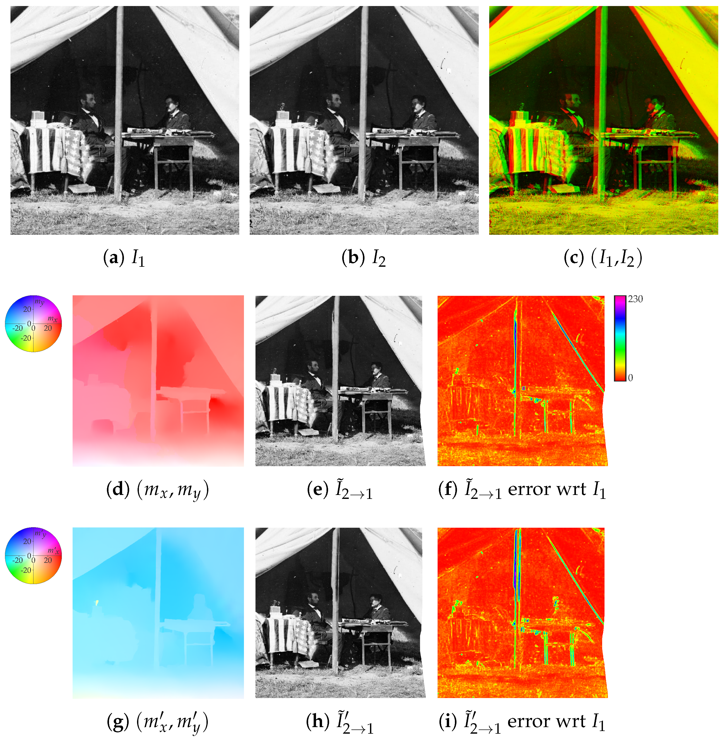
As a first step, the recent state-of-the-art RAFT deep network [16] is used to compute the optical flow map pair , where (see Figure 2d), so that a synthesized image based on the content of and registered onto can be obtained as
by transferring pixel intensity values from into the view given by (see Figure 2e). Note that spots of missing data can be present on when no pixel in maps onto the specific image area, due, for instance, to image occlusions. In the error free ideal case, it must hold that for every correspondence between and . However, in real situations, this may not happen, as shown in Figure 2f reporting the average absolute error between and on local window patches.
Notice also that, in the case of perfectly rectified stereo images, it holds everywhere that . Under this particular setup, in which is denoted as disparity map and is the only map that needs to be estimated, several classical methods have proven to provide good results while being computationally efficient [27]. However, according to our experience [21], these methods are not feasible in the case of degraded historical stereo photos. First, image degradation due to aging and the intrinsic image noise due to the technological limitations of the period decrease the ability of these methods to find the right correspondences. Second, the output of these methods is quite sensitive to the initial configuration of the parameters and, by considering the variability of the historical acquisition setups, each stereo pair would require the human supervision to get even a sub-optimal result. Third, the stereo alignment for the photos under consideration is far from perfect due to the technological limitations of the period, hence both the maps and are to be considered. Hence, our choice fell under the state-of-the-art RAFT that provides a sufficiently good initial estimation of the optical flow maps in most cases.
A further flow mapping pair (see Figure 2g) can be obtained by switching the two input images, which can be employed to synthesize a second image according to
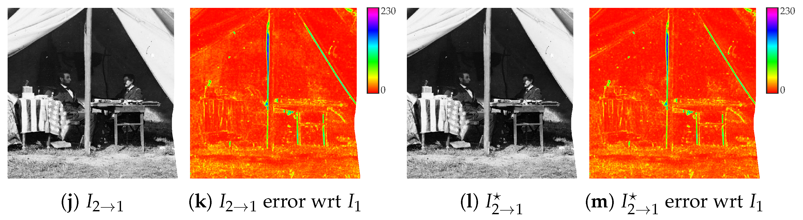
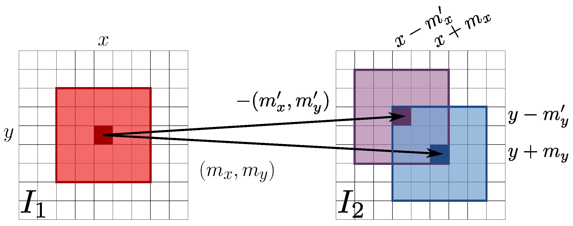
(see Figure 2h) so that, in the error free ideal case for every correspondence between and , it holds that , which implies that . This usually does not happen, as shown by the relative error image of Figure 2i. Indeed, comparing the first and second rows of Figure 2, RAFT optical flow estimation is not completely accurate and does not preserve map inversion when exchanging the input image order. The final synthesized image (see Figure 2j) is then obtained by choosing the intensity value at each pixel as the one from and that minimizes the sum of absolute errors with respect to on a small local window centered on the pixel (see Figure 3). A smaller error between the final resynthesized image and the reference image is obtained (see Figure 2k) with respect to the errors given by and .
2.2. Color Correction
Due to the technical limitations of the old photographic instrumentation, illumination conditions between the two stereo images can differ noticeably. For instance, flash lamp and, even more, flash powder did not provide each time uniform and identical illumination conditions, and it was not infrequent that a single camera was moved in two different positions in order to simulate a stereo setup instead of having two synchronized cameras [21]. Moreover, discoloration of the support due to aging can be present. In order to improve the final result, the state-of-the-art color correction method named Gradient Preserving Spline with Linear Color Propagation (GPS/LCP) presented in [28] is employed to correct the illumination of according to . Specifically, the color map , with is used to obtain the color corrected image according to
where, in the error free ideal case, it must hold that (see Figure 2l). The GPS/LCP color correction method is able to preserve the image content and works also in the case of not perfectly aligned images. Color correction decreases the resynthesis error. This can be noted by comparing the error map of (Figure 2m) with the error map of (Figure 2k), see for instance the error corresponding to the dark background above the left table. Clearly, if presents better illumination conditions than , it is also possible to correct according to .
2.3. Data Fusion
Given the reference image and the synthesized one obtained from the auxiliary view after the illumination post-processing, the two images are blended into a new image according to the stacked median operator (see Figure 4a)
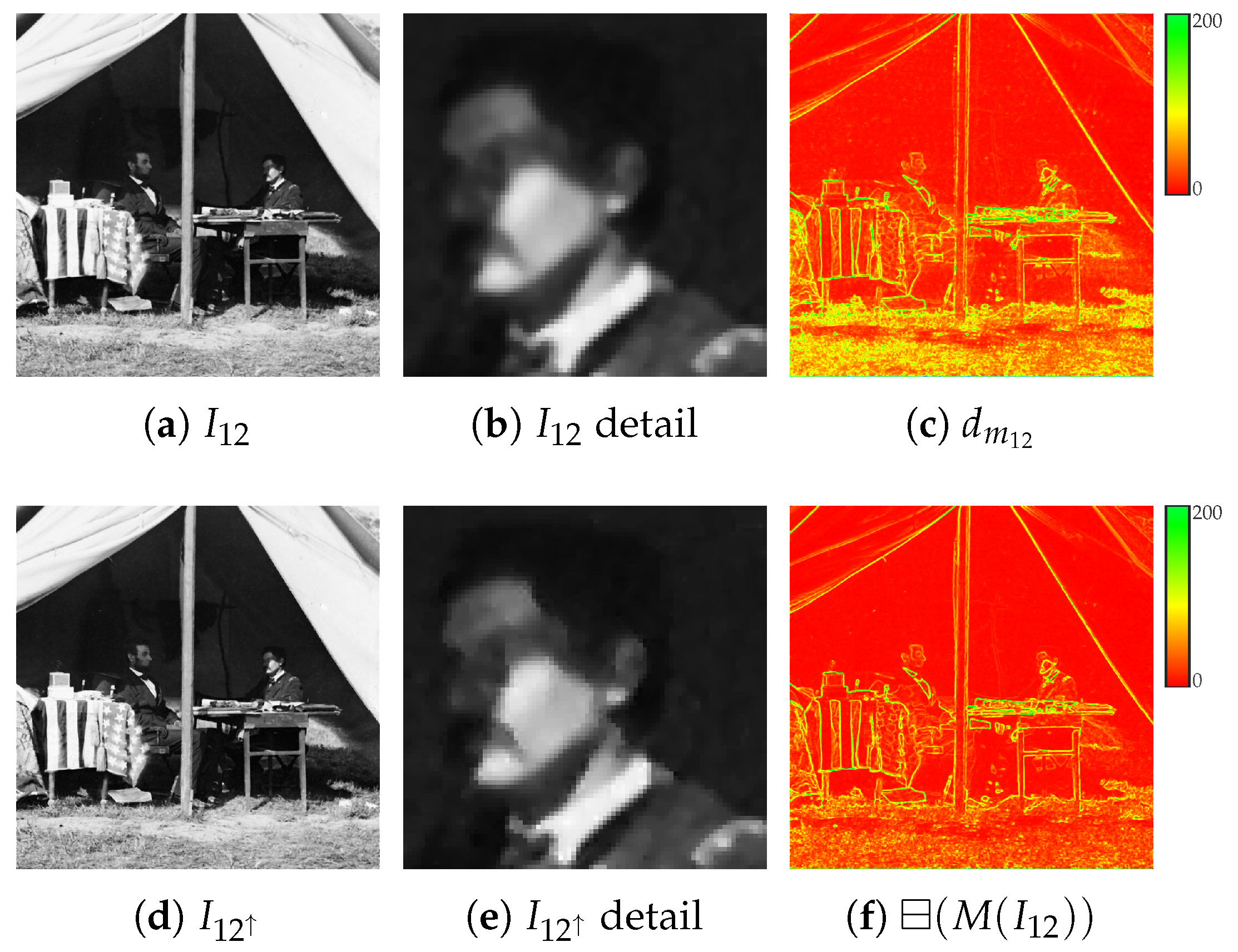
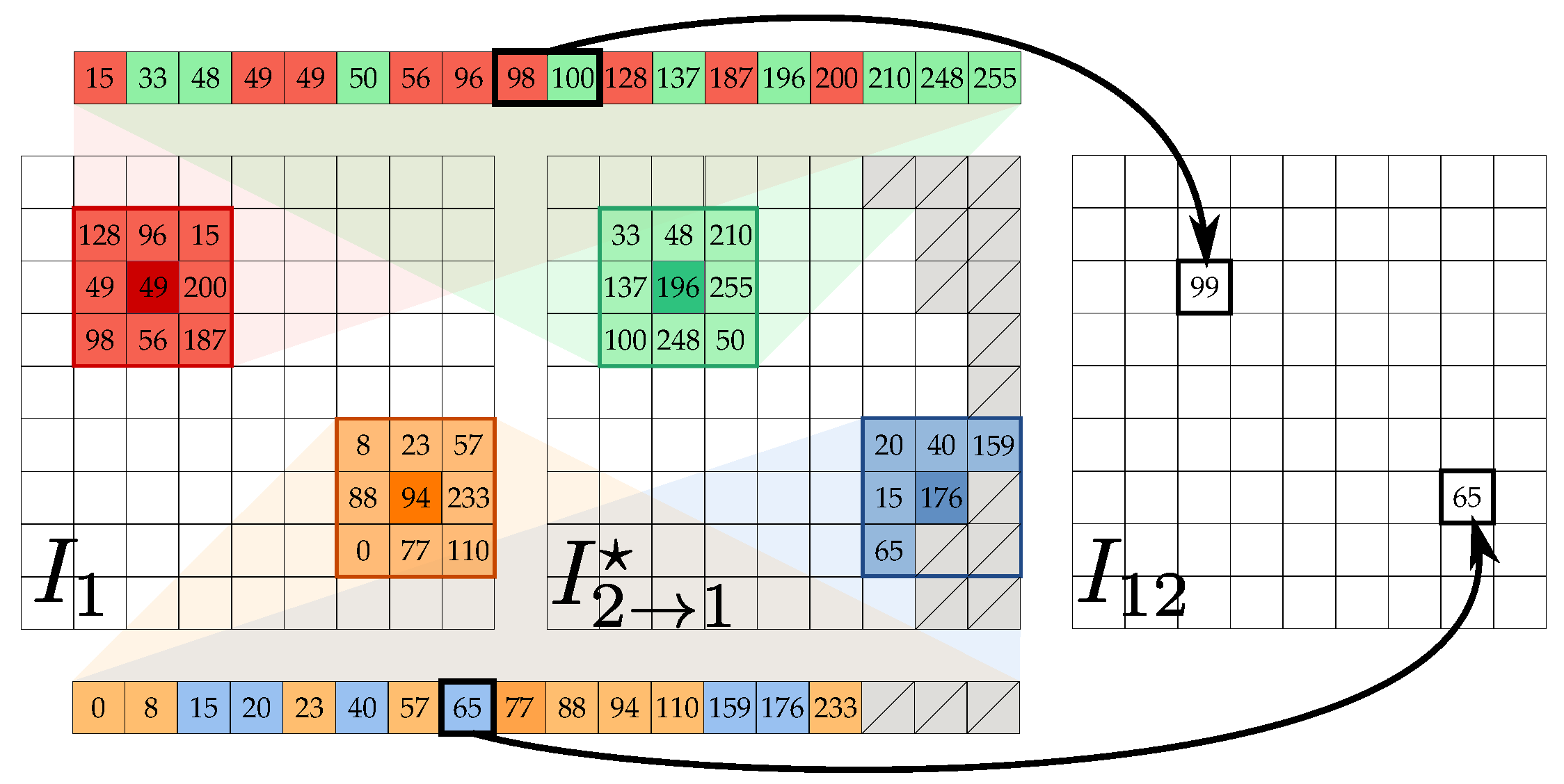
The stacked median for a set of images outputs a new image defined so that image intensity at pixel is the median intensity value computed on the union of the pixels in the local neighbourhood windows centered at on each image of the set (see Figure 5). Notice that the median stacking operation typically found as a blending tool in image manipulation software corresponds to the proposed stacked median operator with degenerate local windows. Unlike median stacking, the proposed definition does not require more than two input images and considers pixel neighborhoods, i.e., it works locally and not pointwise. Additionally, in case of missing data in , the stacked median acts as a standard median filter. With this operator, dirt, scratches and other signs of photographic age or damages are effectively removed from , but high frequency details can be lost in the process, due to the filtering (see Figure 4b). These are partially re-introduced by considering a blended version of the gradient magnitude
(see Figure 4c) obtained as the stacked median of eight possible gradient magnitudes, four for each of the and images, to further enhance finer details. Each gradient magnitude image in the set for a generic image I is computed as
pixelwise, where the image gradient direction pairs are computed by the convolution of I with the following four pairs of kernel filters:
Notice that in the general case (compare Figure 4c with Figure 4f). Consider for now only a single derivative pair of : Each pixel intensity is incremented by a value satisfying
This equation has a twofold solution
In the case of two real solutions, v is chosen as in order to alter as little as possible. In the case of complex solutions, is set to 0. The final gradient-enhanced image is then obtained as
(see Figure 4d,e for details). Since four different v values are obtained for each of the four derivative pairs of Equation (7), their average value is actually employed.
2.4. Refinement
As already noted, the optical flow may be not perfect, causing the presence of wrong data in the image synthesis and hence in the data fusion process described in the previous step. To alleviate this issue, an iterative error-driven image correction step is introduced, where each iteration can be split into two sub-steps:
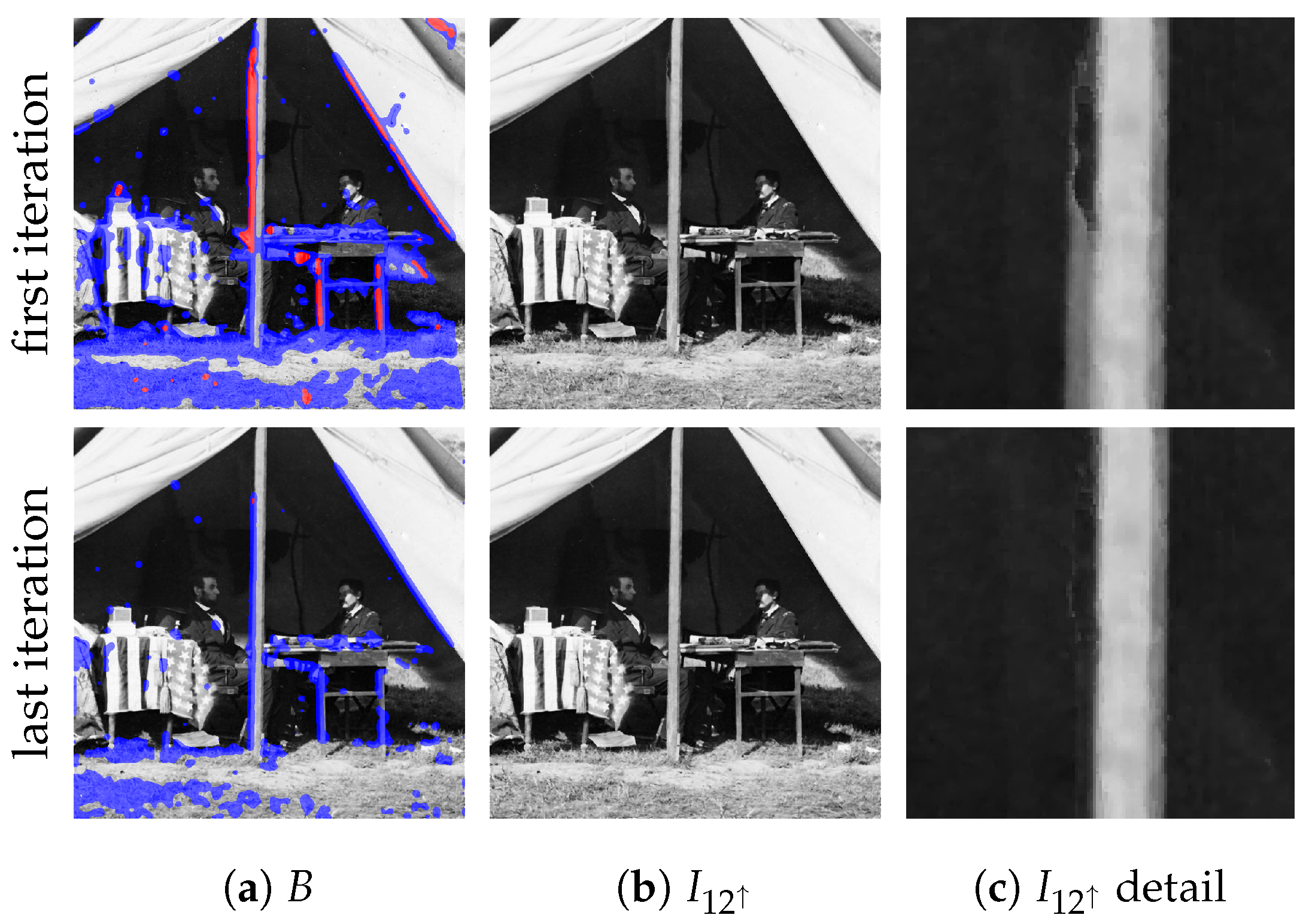
- Detection. A binary correction mask is computed by considering the error image the local window centered at each . Given as the subset of pixels with intensity values lower than the 66% percentile on , the pixel is marked as requiring adjustment if the square root of the average intensity value on is higher than (chosen experimentally). This results in a binary correction mask B that is smoothed with a Gaussian kernel and then binarized again by a threshold value of 0.5. As clear from Figure 6a, using the percentile-based subset is more robust than working with the whole window .
- Adjustment. Data fusion is repeated again after updating pixels on that need to be adjusted with the corresponding ones of . Since is a sort of average between and , the operation just described pushes marked pixels towards . At the end of this step, the gradient enhanced image is also updated accordingly and, in case of no further iterations, it constitutes the final output.
Iterations stop when no more pixels to be adjusted are detected in the updated or when the maximum number of iterations is reached (see Figure 6). A maximum of four iterations is carried out, since it was verified experimentally that data fusion typically converges to within this number of steps.
2.5. Guided Supersampling
Previous steps describe the original SMR implementation [23]. In order to preserve more fine details of the input images, a better image fusion is proposed hereafter, where the original coarse blended image (Equation (4)) is employed to guide a refinement on the basis of supersampling (see Figure 7).
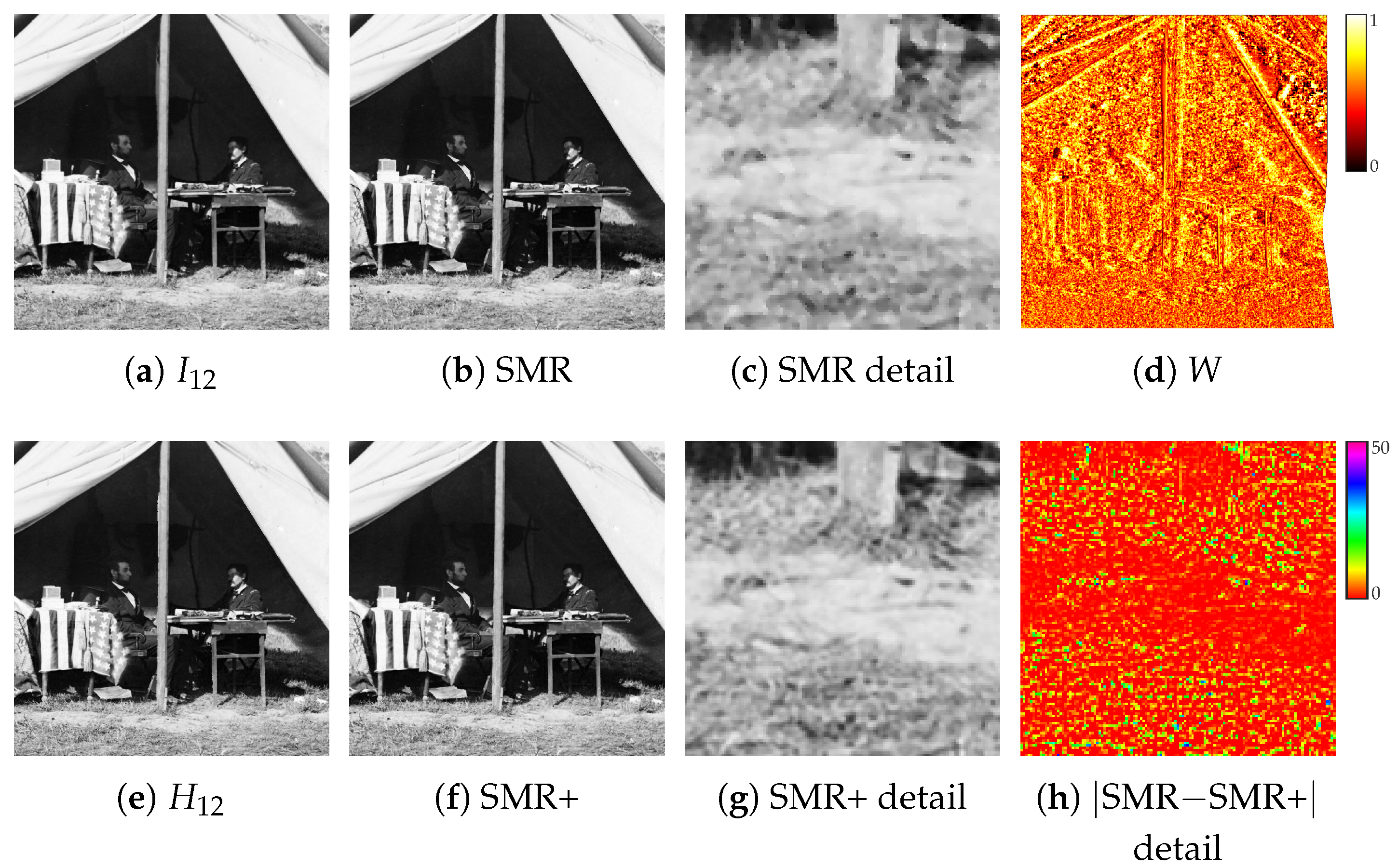
Let denote the image obtained by averaging on a window, and similarly the one obtained with . The weight mask W is computed as pixelwise, followed by the convolution with a Gaussian with a standard deviation of four pixels (see Figure 7d). A value of W close to 0 (1) for a given pixel implies that the local neighborhood of that pixel in () is very likely less noisy and more artefact-free than (). The mask W is used to define a weighted stacked median
where the superscript indicates the bicubic rescaling by a factor two for supersampling (see Figure 7e). Explicitly, the weighted stacked median at is obtained as the median of the intensities of , where is the subset of the pixels in the local neighbourhood of containing the intensity values closest to , with and , and likewise for containing the pixels with the closest values. In other words, the number of considered samples for the median taken from each image is proportional to the weight . The cardinalities of the subsets and for the different weight ranges are explicitly shown in Table 1.
The high resolution blended image replaces in the next steps of the method (see Section 2.3 and Section 2.4), and being also replaced accordingly by and . The final output is scaled down to the original input size. With respect to the original SMR implementation, the use of guided supersampling in SMR+ preserves better fine details, also improving further the restoration process (compare Figure 7c,g). Notice that, after each refinement sub-step (see Section 2.4), the coarse image needed to guide the process is generated by the stacked median between and scaled down to the original size.
3. Evaluation
3.1. Dataset
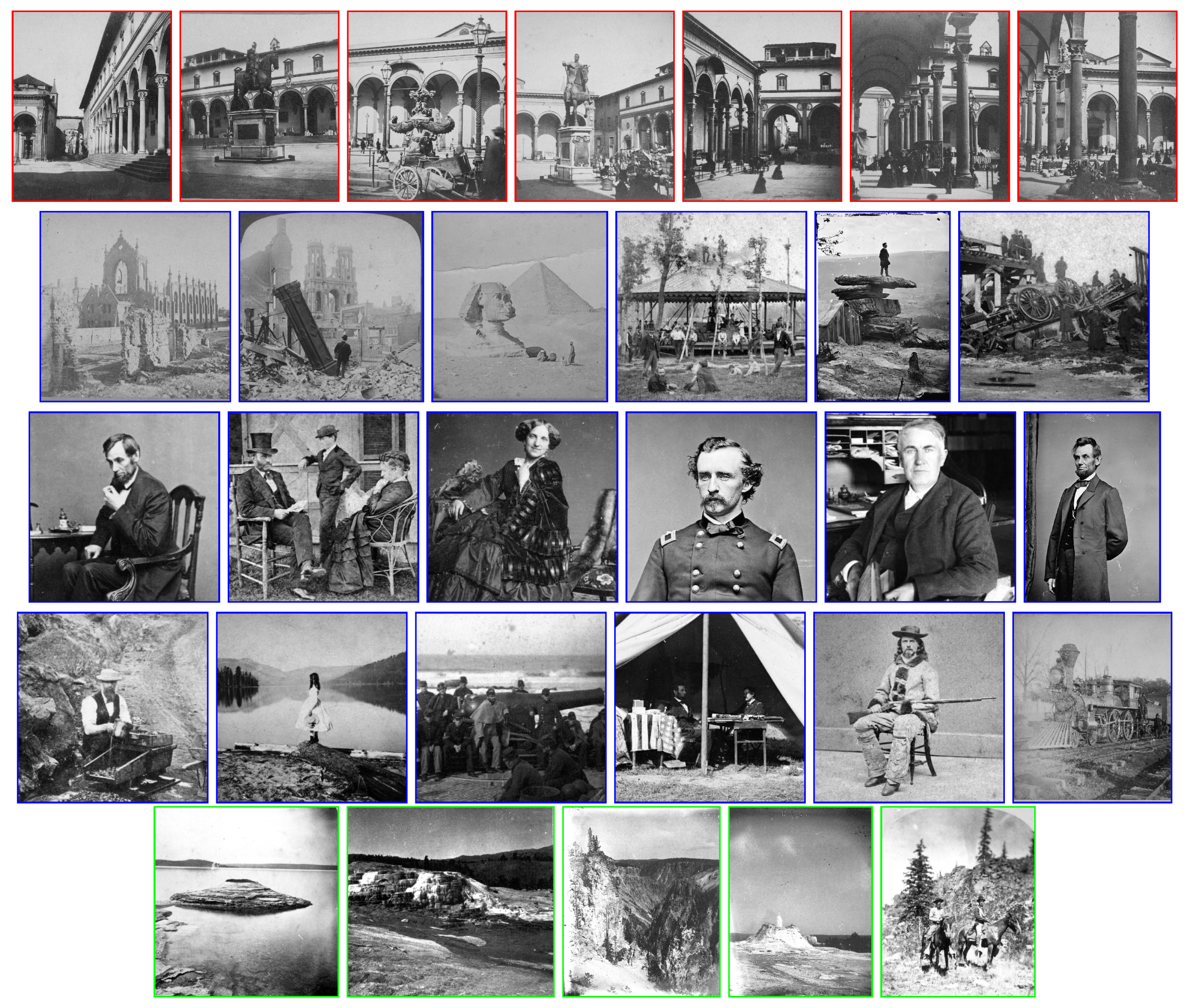
In order to evaluate the proposed approach, we built a new dataset including historical stereo pairs from different sources. The left frames of the selected stereo pairs are shown as reference in Figure 8.
A first set of seven stereo pairs belongs to the collection of stereograms by Anton Hautmann, one of the most active photographers in Florence between 1858 and 1862. Part of Hautmann’s collection is described in [21]. The seven stereo pairs used in this work depict different viewpoints of Piazza Santissima Annunziata in Florence as it was in the middle of the 19th century. Inspecting these photos (see Figure 8, red frames), it can be noticed that the image quality is very poor. In particular, the pairs are quite noisy, with low definition and contrast, include saturated or blurred areas and also show scratches and stains.
A second set includes 35 stereo pairs and increases the original set of ten images employed in [23]. These stereo pairs have been gathered from the Stereoscopic History Instagram account (https://www.instagram.com/stereoscopichistory/, accessed on 1 April 2021, see Figure 8, blue frames for some examples) and contain landscape pictures of urban and natural scenes as well as individual or group portraits. This set is the most challenging one, since its images are heavily corrupted by noise and other artefacts.
A third set of five images was collected from the U.S. Geological Survey (USGS) Historical Stereoscopic Photos account on Flickr (https://www.flickr.com/photos/usgeologicalsurvey/, accessed on 1 April 2021), and represents natural landscapes (see Figure 8, green frames), except for the last one which also includes two horsemen with their mounts. The quality of these images is similar to that of the first set, but strong vignetting effects are also present.
3.2. Compared Methods
The proposed SMR and SMR+ are compared against Block Matching 3D (BM3D) [7], Deep Image Prior (DIP) [13] and the recent BOPBtL [26]. BM3D and DIP are, respectively, a handcrafted and deep generic denoising methods, while BOPBtL is a deep network specifically designed for old photo restoration. These methods currently represent the state-of-the-art in this research area.
For BM3D, the legacy version was employed, since, according to our preliminary experiments, the new version including correlated noise suppression did not work well for our kind of images. The BM3D parameter, the only one present, was set to 7 and 14, values that, according to our experiments, gave the best visual results. In particular, seems to work better than in the case of higher resolution images. Besides applying the standard BM3D on the reference image, a modified version of this method was implemented in order for BM3D to benefit from the stereo auxiliary data. Since BM3D exploits image self-correlation to suppress noise, the modified BM3D generates auxiliary sub-images by placing side by side two corresponding patches from and , then runs the original BM3D on each sub-image and finally generates the output by collecting the blocks from each sub-image corresponding to the central patches. No difference in the results with respect to the standard BM3D was observed, which plausibly implies that corresponding patches for and are not judged as similar to each other by BM3D.
In the case of DIP, the borders of the input images were cropped due to network architectural constraints: These missing parts were replaced with content from the original input images.
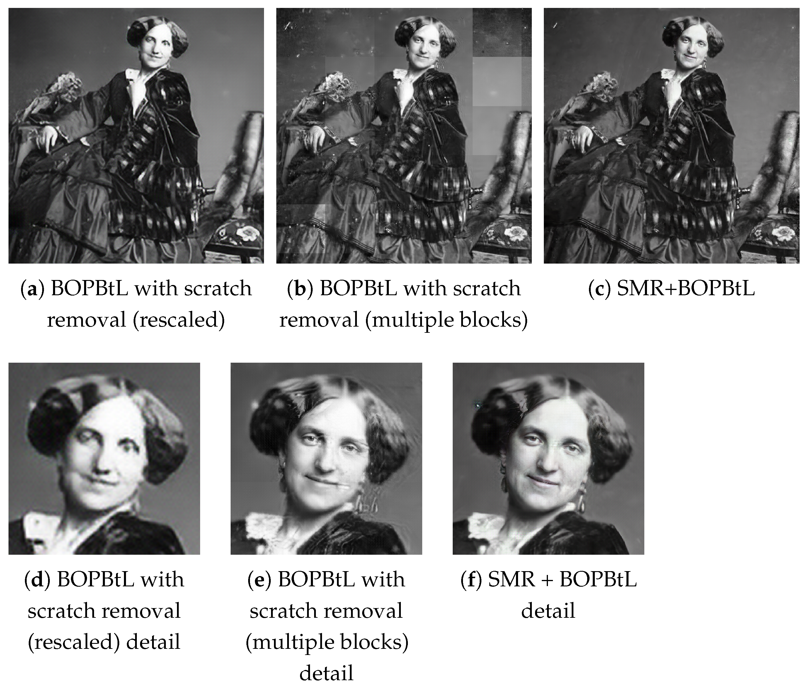
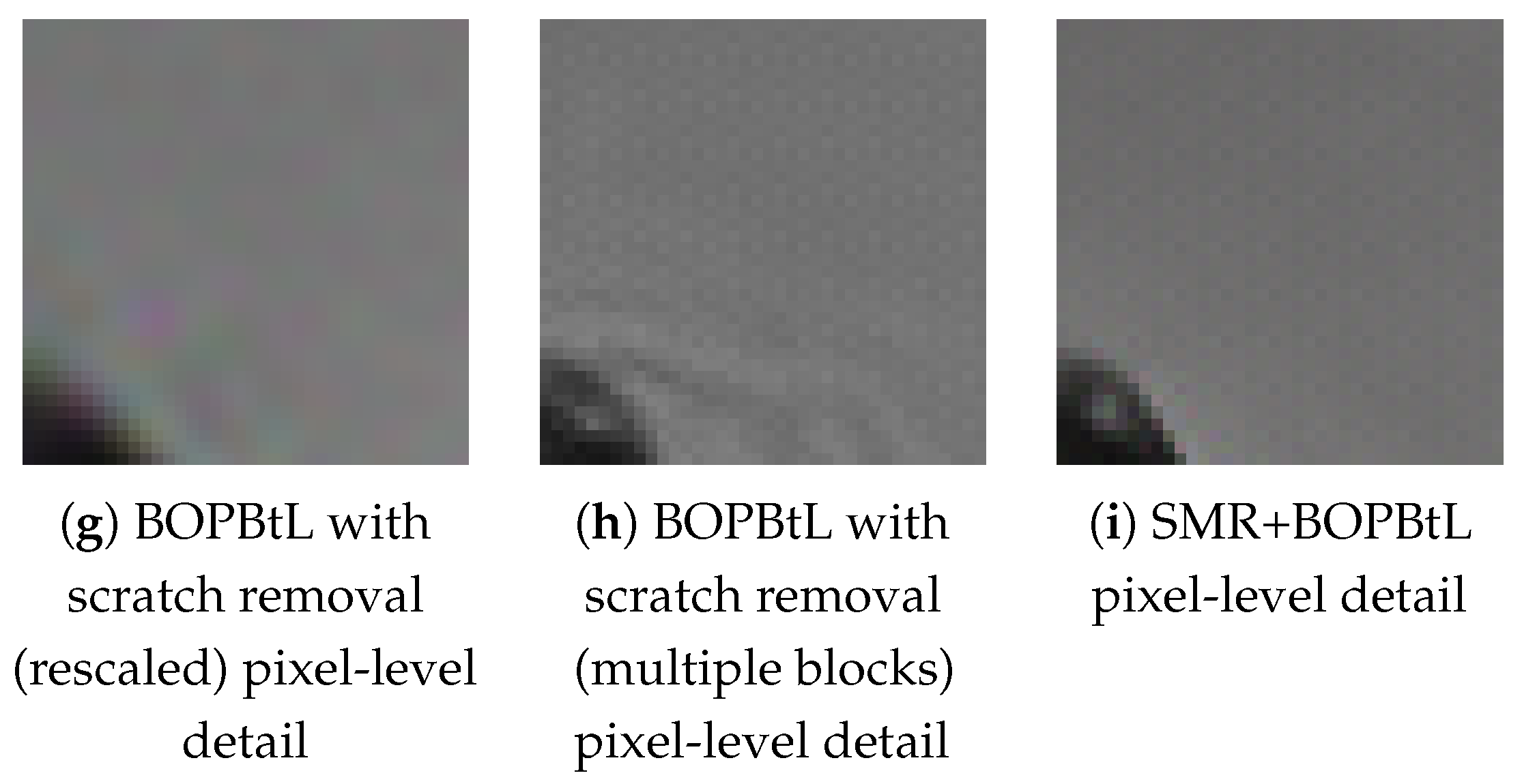
Concerning BOPBtL, the scratch removal option was disabled since it caused the network to crash. This is a known issue related to the high memory requirement exceeding the standard 12 GB GPU amount to run the network on standard image input (https://github.com/microsoft/Bringing-Old-Photos-Back-to-Life/issues/, accessed on 1 April 2021), and does not occur only when the input image size is small. To circumvent this problem, two solutions were attempted, yet without satisfying results. Specifically, in the first solution, the input image was rescaled to a fixed size (from 50% to 33% of the its original size), but the final result lost too many details (see Figure 9a). In the second solution, the input was processed in separated blocks, causing a lack of global consistency in the output (see Figure 9b). Moreover, in both solutions, the chessboard artefact effect, typical of many deep networks that resynthesize images, looked more evident than in the original BOPBtL implementation. BOPBtL was employed to post-process the output of SMR+, which was denoted as SMR+BOPBtL in the results (see Figure 9c).
3.3. Results
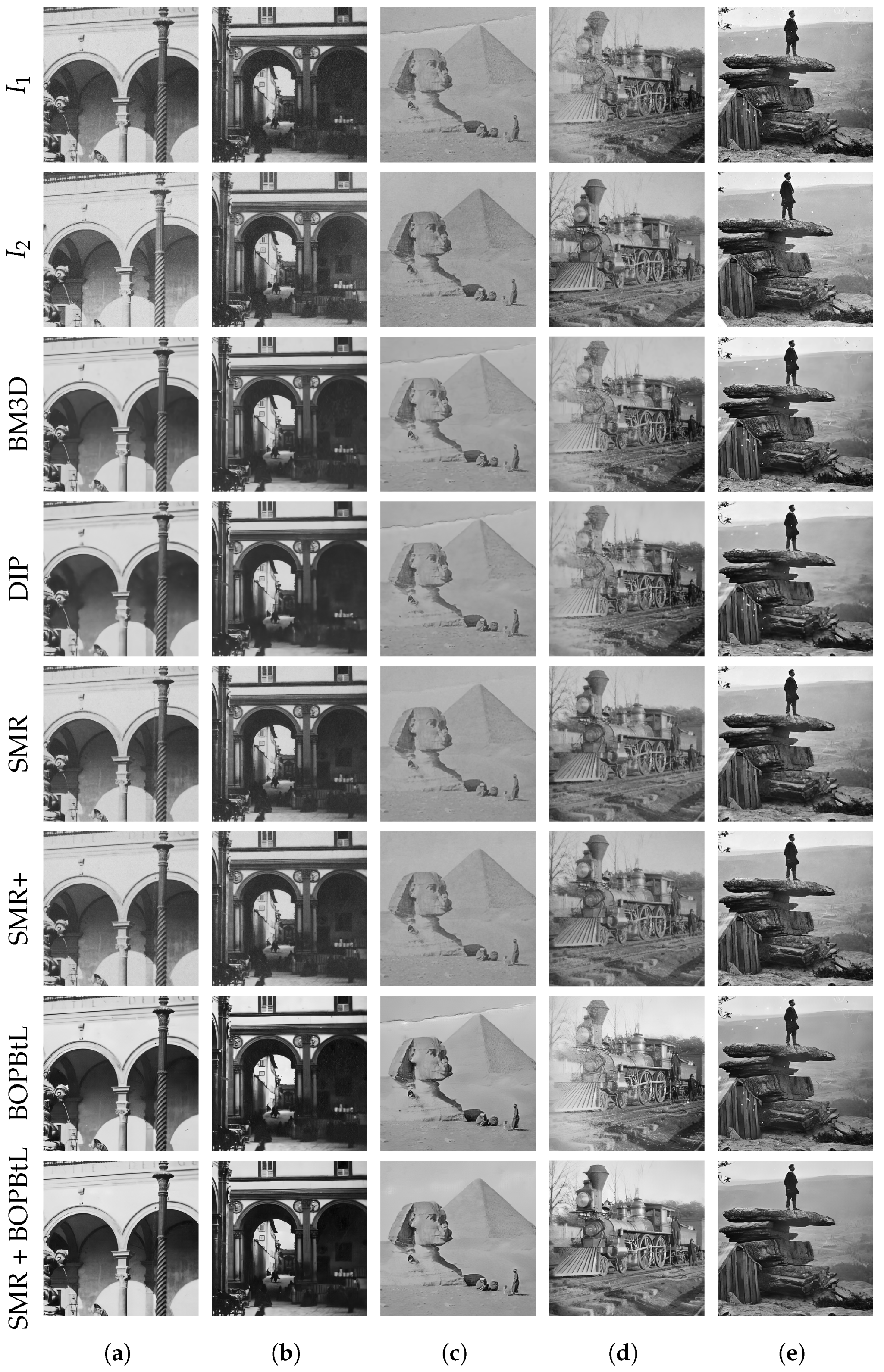
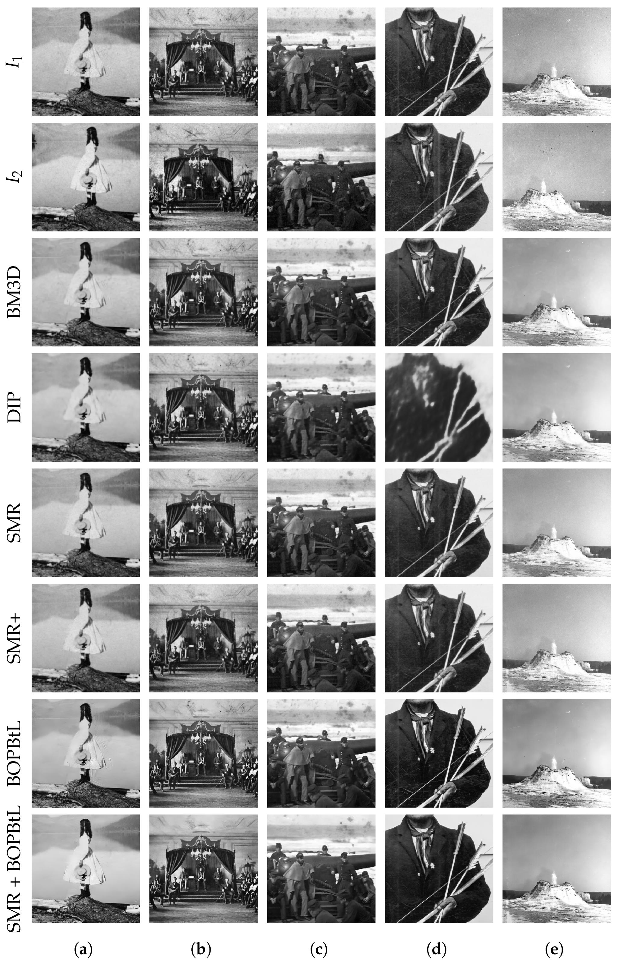
Figure 10 and Figure 11 show some examples of the results obtained with the compared methods. For a thorough visual qualitative evaluation, the reader is invited to inspect the full-resolution results obtained on the whole dataset, which are included in the additional material (https://drive.google.com/drive/folders/1Fmsm50bMMDSd0z4JXOhCZ3hPDIXdwMUL). From a direct visual inspection of the results, BM3D and DIP often seem to oversmooth relevant details in the image, with BM3D producing somewhat better results than DIP, which sometimes simply fails to obtain a reasonable output (see Figure 11d, row DIP). BOPBtL is able to bring out fine details, providing altogether a locally adaptive smoothing and contrast enhancement of the image, with satisfactory results. Nevertheless, none of the previous methods is able to detect and compensate for dust, scratches and other kinds of artefacts that conversely may even be amplified in the restoration process, as one can check by locating dust spots and sketches in Figure 10e, rows BM3D, DIP and BOPBtL. This problem is mostly evident for BOPBtL, where image artefacts are heavily boosted together with finer details.
Conversely, SMR-based methods are able to solve these issues by exploiting the additional information present in the auxiliary image, with the exception of very severe conditions such as the stains appearing in the right skyline of Figure 11c, for which, anyways, SMR-based methods still get the best restoration of all. SMR-based methods also successfully enhance the image contrast, as it happens for the window in the dark spot under the right arcade in Figure 10b, rows SMR and SMR+. When image degradations are even more severe than that, good results can nevertheless be obtained by forcing the illumination of the auxiliary image into the reference (see Section 2.2), as done for Figure 10d, rows SMR, SMR+ and SMR+BOPBtL. Concerning the guided supersampling introduced for SMR+, this is able not only to preserve high frequency details (see again Figure 7), but also to better clean-up the image, as one can notice by inspecting the removed scratch from Figure 10c, row SMR+. Guided supersampling also alleviates spurious artefacts arising from inaccurate optical flow estimation as in the case of the light pole of Figure 10a (compare rows SMR and SMR+). Only in few cases of very inaccurate optical flow estimation is SMR+ unable to fix inconsistencies and generates some spurious artefacts as in the bottom-left white scratch in Figure 11e, rows SMR+ and SMR + BOPBtL. Finally, it can be noted that SMR + BOPBtL is able to take the best from both the methods, i.e., the artefact removal from SMR+ and the image enhancement from BOPBtL, and provides very visually striking results.
Table 2 reports the score obtained by the compared methods on the images discussed so far according to popular no-reference quality assessment metrics. Specifically, scores are reported for the Blind/Referenceless Image Spatial Quality Evaluator (BRISQUE) [29], the Naturalness Image Quality Evaluator (NIQE) [30] and Perception based Image Quality Evaluator (PIQE) [31]. Due to the lack of ground-truth clean data and of a well-defined image model for the generation of synthetic images with the same characteristics of the input image under evaluation, image quality measurements requiring a reference image such as the Structural Similarity Index (SSIM) [32] cannot be applied. By inspection of the scores obtained, it clearly emerges that these quality metrics do not reflect the human visual judgment, hence they are unsuitable for a reliable quantitative evaluation in this specific application scenario. In particular, there is no agreement among the various metrics and, in about half of the cases, the input image even gets a better score than the restored one, in contrast with the human visual assessment. Furthermore, SMR+ and SMR + BOPBtL obtain worse scores than the original images or BOPBtL in the cases where SMR-methods successfully cleaned the image by removing strong image artefacts, again in contrast with human judgment (see Figure 11b,d). A possible explanation of this behavior is that these metrics only rely on low-level, local image properties and not on high-level, semantic image characteristics. Hence, they are unable to distinguish between fine image details and artefacts. Nevertheless, according to Table 2, SMR+, with or without BOPBtL, shows good results under these blind quality assessment metrics, implying that it is able not only to remove structural artefacts from the original image, but also to maintain high quality visual details besides the semantic interpretation of the scene.
Concerning running times, BM3D, BOPBtL and DIP require respectively 10 s, 30 s and 20 min on average for processing the dataset images, while SMR and SMR+ take respectively 6 min and 9 min. The running environment is a Ubuntu 20.04 system running on an Intel Core i7-3770K with 8 GB of RAM equipped with a 12 GB NVIDIA Titan XP. BM3D is a Matlab optimized .mex file, BOPBtL and DIP implementations run on Pytorch exploiting GPU acceleration, while, with the exception of RAFT optical flow estimation, SMR and SMR+ are based on non-optimized Matlab code running on CPU. For both SMR and SMR+ the times include the image resynthesis and color correction steps that take 4.5 min altogether on average. Under these considerations, both SMR and SMR+ running times are reasonable for offline applications. None of the compared methods can be used for real-time applications, as in the best case corresponding to BM3D, 10 s are required for processing the input image.
4. Conclusions and Future Work
This paper proposed a novel method for the fully automatic restoration of historical stereo photographs. By exploiting optical flow, the auxiliary view of the stereo frame is geometrically and photometrically registered onto the reference view. Restoration is then carried out by fusing the data from both images according to our stacked median approach followed by gradient adjustments aimed at preserving details. Guided supersampling is also introduced and successfully applied for enhancing finer details and simultaneously providing a more effective artefact removal. Finally, an iterative refinement step driven by a visual consistency check is performed in order to remove the artefacts due to optical flow estimation errors in the initial phase.
Results on several historical stereo pairs show the effectiveness of the proposed approach that is able to remove most of the image defects including dust and scratches, without excessive smoothing of the image content. The approach works better than its single-image denoising competitors, thanks to the ability of exploiting stereo information. As a matter of fact, single-image methods have severe limitations in handling damaged areas, and usually produce more blurry results. Nevertheless, experimental results show that single image BOPBtL, when cascaded with our approach into SMR + BOPBtL, can achieve remarkably good performances.
Future work will investigate novel solutions to refine the optical flow in order to reduce pixel mismatches. A further research direction will be towards consolidating the stacked median approach as an image blending technique. Finally, the proposed method will be extended and adapted to the digital restoration of historical films.
Author Contributions
Conceptualization, F.B.; methodology, F.B. and M.F.; software, F.B and M.F.; validation, F.B., M.F. and C.C.; formal analysis, F.B., M.F. and C.C.; investigation, F.B. and M.F.; resources, F.B., M.F. and C.C.; data curation, F.B., M.F. and C.C.; writing—original draft preparation, F.B.; writing—review and editing, M.F., C.C. and F.B.; visualization, F.B., M.F. and C.C.; supervision, F.B. and C.C.; project administration, F.B. and C.C.; funding acquisition, F.B. All authors have read and agreed to the published version of the manuscript.
Funding
This work was supported by the Italian Ministry of University and Research (MUR) under the program PON Ricerca e Innovazione 2014–2020, cofunded by the European Social Fund (ESF), CUP B74I18000220006, id. proposta AIM 1875400, linea di attività 2, Area Cultural Heritage.
Institutional Review Board Statement
Not applicable.
Informed Consent Statement
Not applicable.
Data Availability Statement
Additional material including code, dataset and evaluation results are freely available online at https://drive.google.com/drive/folders/1Fmsm50bMMDSd0z4JXOhCZ3hPDIXdwMUL.
Acknowledgments
The Titan Xp used for this research was generously donated by the NVIDIA Corporation. We would like to thank Costanza Caraffa and Ute Dercks at Photothek des Kunsthis torischen Instituts in Florenz–Max-Planck-Institut for allowing the reproduction of the photos in this paper. Hautmann’s collection digital scans: ©Stefano Fancelli/KHI.
Conflicts of Interest
The authors declare no conflict of interest. The funders had no role in the design of the study; in the collection, analyses, or interpretation of data; in the writing of the manuscript, or in the decision to publish the results.
References
- Ardizzone, E.; De Polo, A.; Dindo, H.; Mazzola, G.; Nanni, C. A Dual Taxonomy for Defects in Digitized Historical Photos. In Proceedings of the 10th International Conference on Document Analysis and Recognition, Barcelona, Spain, 26–29 July 2009; pp. 1166–1170. [Google Scholar]
- Kokaram, A.C. Motion Picture Restoration: Digital Algorithms for Artefact Suppression in Degraded Motion Picture Film and Video; Springer: Berlin/Heidelberg, Germany, 1998. [Google Scholar]
- Tegolo, D.; Isgrò, F. A genetic algorithm for scratch removal in static images. In Proceedings of the International Conference on Image Analysis and Processing (ICIAP2001), Palermo, Italy, 26–28 September 2001; pp. 507–511. [Google Scholar]
- Stanco, F.; Tenze, L.; Ramponi, G. Virtual restoration of vintage photographic prints affected by foxing and water blotches. J. Electron. Imaging 2005, 14, 043008. [Google Scholar] [CrossRef]
- Besserer, B.; Thiré, C. Detection and Tracking Scheme for Line Scratch Removal in an Image Sequence. In Proceedings of the European Conference on Computer Vision (ECCV2004), Prague, Czech Republic, 11–14 May 2004; pp. 264–275. [Google Scholar]
- Criminisi, A.; Perez, P.; Toyama, K. Object removal by exemplar-based inpainting. In Proceedings of the IEEE Conference on Computer Vision and Pattern Recognition (CVPR2003), Madison, WI, USA, 16–22 June 2003; Volume 2. [Google Scholar]
- Dabov, K.; Foi, A.; Katkovnik, V.; Egiazarian, K. Image Denoising by Sparse 3D Transform-Domain Collaborative Filtering. IEEE Trans. Image Process. 2007, 16, 2080–2095. [Google Scholar] [CrossRef] [PubMed]
- Chen, F.; Zhang, L.; Yu, H. External Patch Prior Guided Internal Clustering for Image Denoising. In Proceedings of the IEEE International Conference on Computer Vision (ICCV2015), Santiago, Chile, 7–13 December 2015; pp. 603–611. [Google Scholar]
- Buades, A.; Lisani, J.; Miladinović, M. Patch-Based Video Denoising With Optical Flow Estimation. IEEE Trans. Image Process. 2016, 25, 2573–2586. [Google Scholar] [CrossRef]
- Nasrollahi, K.; Moeslund, T.B. Super-resolution: A comprehensive survey. Mach. Vis. Appl. 2014, 25, 1423–1468. [Google Scholar] [CrossRef] [Green Version]
- Yang, J.; Wright, J.; Huang, T.S.; Ma, Y. Image Super-Resolution Via Sparse Representation. IEEE Trans. Image Process. 2010, 19, 2861–2873. [Google Scholar] [CrossRef] [PubMed]
- Castellano, G.; Vessio, G. Deep learning approaches to pattern extraction and recognition in paintings and drawings: An overview. Neural Comput. Appl. 2021. [Google Scholar] [CrossRef]
- Ulyanov, D.; Vedaldi, A.; Lempitsky, V. Deep Image Prior. In Proceedings of the IEEE Conference on Computer Vision and Pattern Recognition (CVPR2018), Salt Lake City, UT, USA, 18–23 June 2018. [Google Scholar]
- Wang, Z.; Chen, J.; Hoi, S.C.H. Deep Learning for Image Super-resolution: A Survey. IEEE Trans. Pattern Anal. Mach. Intell. 2020. [Google Scholar] [CrossRef] [PubMed] [Green Version]
- Zhang, Y.; Tian, Y.; Kong, Y.; Zhong, B.; Fu, Y. Residual Dense Network for Image Restoration. IEEE Trans. Pattern Anal. Mach. Intell. 2021, 43, 2480–2495. [Google Scholar] [CrossRef] [Green Version]
- Teed, Z.; Deng, J. RAFT: Recurrent All-Pairs Field Transforms for Optical Flow. In Proceedings of the European Conference on Computer Vision (ECCV2020, Glasgow, UK, 23–28 August 2020. [Google Scholar]
- Jeon, D.S.; Baek, S.; Choi, I.; Kim, M.H. Enhancing the Spatial Resolution of Stereo Images Using a Parallax Prior. In Proceedings of the IEEE Conference on Computer Vision and Pattern Recognition (CVPR2018), Salt Lake City, UT, USA, 18–23 June 2018; pp. 1721–1730. [Google Scholar]
- Zhou, S.; Zhang, J.; Zuo, W.; Xie, H.; Pan, J.; Ren, J.S. DAVANet: Stereo Deblurring With View Aggregation. In Proceedings of the IEEE Conference on Computer Vision and Pattern Recognition (CVPR2019), Long Beach, CA, USA, 16–20 June 2019; pp. 10988–10997. [Google Scholar]
- Yan, B.; Ma, C.; Bare, B.; Tan, W.; Hoi, S. Disparity-Aware Domain Adaptation in Stereo Image Restoration. In Proceedings of the IEEE Conference on Computer Vision and Pattern Recognition (CVPR2020), Seattle, WA, USA, 14–18 June 2020; pp. 13176–13184. [Google Scholar]
- Schindler, G.; Dellaert, F. 4D Cities: Analyzing, Visualizing, and Interacting with Historical Urban Photo Collections. J. Multimed. 2012, 7, 124–131. [Google Scholar] [CrossRef] [Green Version]
- Fanfani, M.; Bellavia, F.; Bassetti, G.; Argenti, F.; Colombo, C. 3D Map Computation from Historical Stereo Photographs of Florence. IOP Conf. Ser. Mater. Sci. Eng. 2018, 364, 012044. [Google Scholar] [CrossRef]
- Luo, X.; Kong, Y.; Lawrence, J.; Martin-Brualla, R.; Seitz, S. KeystoneDepth: Visualizing History in 3D. arXiv 2019, arXiv:1908.07732. [Google Scholar]
- Fanfani, M.; Colombo, C.; Bellavia, F. Restoration and Enhancement of Historical Stereo Photos through Optical Flow. In Proceedings of the ICPR Workshop on Fine Art Pattern Extraction and Recognition (FAPER), Milan, Italy, 18 September 2021. [Google Scholar]
- McCann, J.J.; Rizzi, A. The Art and Science of HDR Imaging; John Wiley & Sons Inc.: Chichester, UK, 2011. [Google Scholar]
- Sherrod, A. Game Graphic Programming; Course Technology: Boston, MA, USA, 2008. [Google Scholar]
- Wan, Z.; Zhang, B.; Chen, D.; Zhang, P.; Chen, D.; Liao, J.; Wen, F. Bringing Old Photos Back to Life. In Proceedings of the IEEE/CVF Conference on Computer Vision and Pattern Recognition (CVPR), Seattle, WA, USA, 14–18 June 2020. [Google Scholar]
- Chambon, S.; Crouzil, A. Similarity measures for image matching despite occlusions in stereo vision. Pattern Recognit. 2011, 44, 2063–2075. [Google Scholar] [CrossRef]
- Bellavia, F.; Colombo, C. Dissecting and Reassembling Color Correction Algorithms for Image Stitching. IEEE Trans. Image Process. 2018, 27, 735–748. [Google Scholar] [CrossRef]
- Mittal, A.; Moorthy, A.K.; Bovik, A.C. No-Reference Image Quality Assessment in the Spatial Domain. IEEE Trans. Image Process. 2012, 21, 4695–4708. [Google Scholar] [CrossRef] [PubMed]
- Mittal, A.; Soundararajan, R.; Bovik, A.C. Making a “Completely Blind” Image Quality Analyzer. IEEE Signal Process. Lett. 2013, 20, 209–212. [Google Scholar] [CrossRef]
- Venkatanath, N.; Praneeth, D.; Chandrasekhar, B.; Channappayya, S.; Medasani, S. Blind image quality evaluation using perception based features. In Proceedings of the 21st National Conference on Communications (NCC), Mumbai, India, 27 February–1 March 2015; pp. 1–6. [Google Scholar]
- Wang, Z.; Bovik, A.C.; Sheikh, H.R.; Simoncelli, E.P. Image quality assessment: From error visibility to structural similarity. IEEE Trans. Image Process. 2004, 13, 600–612. [Google Scholar] [CrossRef] [PubMed] [Green Version]
Figure 1.
First row: An example of historical stereo pair of images, and , also superimposed as anaglyph. Second row: Enhancement of according to different methods, including the proposed SMR+ method. Although visually impressive, the deep super-resolution result of BOPBtL does not preserve the true input image. Third row: A detail of and the restored images according to the different methods. A closer look at BOPBtL reveals alterations with respect to the original face expression, accentuating the smile and introducing bush-like textures on the hair. Fourth row: pixel level detail of and of the restored images according to the different methods. The specific image region considered is the background around the right shoulder. Notice the chessboard-like texture pattern typical of the deep network approaches, not visible at coarser scales. Best viewed in color: the reader is invited to zoom in on the electronic version of the manuscript in order to better appreciate the visual differences.

Figure 2.
Auxiliary image pointwise transfer and color correction steps (see Section 2.1 and Section 2.2): (a) Reference image , (b) auxiliary image , (c) superimposition of and as anaglyph, (d) visual representation of the optical flow map extracted by RAFT, (e) image as resynthesis of through and (f) its error with respect to , (g) visual representation of the optical flow map extracted by RAFT after switching the input images, (h) image as resynthesis from through and (i) its error with respect to , (j) final resynthesized image considering the locally best optical flow estimation between and and (k) its error with respect to , (l) image obtained after applying GPS/LCP color correction to using as reference, and (m) the corresponding error map with respect to . Best viewed in color. The reader is invited to zoom into the electronic version of the manuscript in order to better appreciate the visual differences.


Figure 3.
Illustration of the image formation process from the two resynthesized images and , respectively driven by the optical flow estimation maps and . A point in can be mapped back to according to either Equation (1) or Equation (2). The best back-mapping minimizing locally the error among the two possible optical flow estimates is then chosen to form . Best viewed in color.

Figure 4.
Data fusion step (see Section 2.3): (a) stacked median obtained from , (b) details of , (c) the stacked median of the gradient magnitudes of and , (d) the gradient-enhanced image , (e) a detail of , (f) the gradient magnitude of the stacked median image . Best viewed in color. The reader is invited to zoom in on the electronic version of the manuscript in order to better appreciate the visual differences.

Figure 5.
Application of the stacked median operator ⊟ for computing from . At pixel , the stacked median operator takes the union of the corresponding local neighbourhoods for each image of the input set (in the example, the union of the red and green neighbourhoods, and the union of the orange and blue ones, missing data are represented in the figure as gray ticked boxes) and assigns its median intensity value to the point in the new image. Best viewed in color.

Figure 6.
Refinement step (see Section 2.4). First (top row) and last (bottom row) iterations of the detection and adjustment sub-steps. (a) detection mask B at the beginning of the iteration, (b) updated at the end of the iteration and (c) details of (b). Pixels to be adjusted using (L) are underlined in the images by saturating the red (blue) channel. By inspecting the details, it can be seen that the ghosting effect is removed. Best viewed in color. The reader is invited to zoom in on the electronic version of the manuscript in order to better appreciate the visual differences.

Figure 7.
Guided supersampling step (see Section 2.5): (a) SMR stacked median , (b) final restored image and (c) details of it, (d) weight mask W for the guided supersampling, (e) SMR+ weighted stacked median , (f) final restored image, (g) a detail of it, and (h) its differences with respect to the SMR output. Best viewed in color. The reader is invited to zoom in on the electronic version of the manuscript in order to better appreciate the visual differences.

Figure 8.
Left frames for some historical stereo pairs. Image frames for Hautmann’s, Stereoscopic Photos and USGS datasets are framed, respectively, in red, blue and green. Best viewed in color and zoomed in with the electronic version of the manuscript.
Figure 8.
Left frames for some historical stereo pairs. Image frames for Hautmann’s, Stereoscopic Photos and USGS datasets are framed, respectively, in red, blue and green. Best viewed in color and zoomed in with the electronic version of the manuscript.

Figure 9.
Results of BOPBtL with scratch removal or in combination with SMR+ on the same stereo pair of Figure 1. Notice that the visual pleasant results of (a) are due to the frequency cutoff caused by rescaling and disappear at a larger viewing scale such in (d). Best viewed in color. The reader is invited to zoom in on the electronic version of the manuscript in order to better appreciate the visual differences.


Figure 10.
Qualitative visual comparison of the methods under test. Best viewed in color. The reader is invited to zoom in on the electronic version of the manuscript in order to better appreciate the differences.
Figure 10.
Qualitative visual comparison of the methods under test. Best viewed in color. The reader is invited to zoom in on the electronic version of the manuscript in order to better appreciate the differences.

Figure 11.
Qualitative visual comparison of the methods under test. Best viewed in color. The reader is invited to zoom in on the electronic version of the manuscript in order to better appreciate the differences.
Figure 11.
Qualitative visual comparison of the methods under test. Best viewed in color. The reader is invited to zoom in on the electronic version of the manuscript in order to better appreciate the differences.


Table 1.
The cardinality of the sets and according to the weight range (see Section 2.5).
Table 1.
The cardinality of the sets and according to the weight range (see Section 2.5).
| 0.00 | 0.05 | 0.11 | 0.16 | 0.21 | 0.26 | 0.32 | 0.37 | 0.42 | 0.47 | 0.53 | 0.58 | 0.63 | 0.68 | 0.74 | 0.79 | 0.84 | 0.89 | 0.95 | |
| 0.05 | 0.11 | 0.16 | 0.21 | 0.26 | 0.32 | 0.37 | 0.42 | 0.47 | 0.53 | 0.58 | 0.63 | 0.68 | 0.74 | 0.79 | 0.84 | 0.89 | 0.95 | 1.00 | |
| 9 | 9 | 9 | 9 | 9 | 9 | 9 | 9 | 9 | 9 | 8 | 7 | 6 | 5 | 4 | 3 | 2 | 1 | 0 | |
| 0 | 1 | 2 | 3 | 4 | 5 | 6 | 7 | 8 | 9 | 9 | 9 | 9 | 9 | 9 | 9 | 9 | 9 | 9 |
Table 2.
No-reference assessment metric results (lower values are better). Values in bold indicate the best score among the compared methods. Scores that are better in the original images than in the restored ones are underlined.
Table 2.
No-reference assessment metric results (lower values are better). Values in bold indicate the best score among the compared methods. Scores that are better in the original images than in the restored ones are underlined.
| BM3D | DIP | SMR | SMR+ | BOPBtL | SMR+ BOPBtL | |||
|---|---|---|---|---|---|---|---|---|
| Figure 1 and Figure 9 | BRISQUE | 41.89 | 54.34 | 51.47 | 53.11 | 43.46 | 24.15 | 24.20 |
| NIQE | 4.23 | 5.31 | 5.31 | 5.09 | 3.98 | 4.09 | 4.24 | |
| PIQE | 45.97 | 78.93 | 85.33 | 50.60 | 46.35 | 22.55 | 25.90 | |
| Figure 10a | BRISQUE | 10.74 | 46.03 | 31.11 | 42.18 | 33.06 | 25.41 | 31.37 |
| NIQE | 2.79 | 3.83 | 3.94 | 3.28 | 3.76 | 4.05 | 4.08 | |
| PIQE | 25.02 | 79.24 | 81.50 | 43.32 | 28.09 | 38.50 | 35.35 | |
| Figure 10b | BRISQUE | 9.84 | 48.68 | 35.95 | 41.57 | 29.69 | 14.17 | 34.69 |
| NIQE | 3.16 | 4.07 | 3.92 | 2.92 | 3.34 | 3.65 | 4.01 | |
| PIQE | 29.73 | 78.53 | 78.16 | 37.26 | 23.61 | 29.98 | 34.31 | |
| Figure 10c | BRISQUE | 9.26 | 44.97 | 31.28 | 38.29 | 33.94 | 12.13 | 19.06 |
| NIQE | 2.79 | 4.22 | 4.11 | 3.47 | 4.04 | 5.43 | 5.31 | |
| PIQE | 15.80 | 60.33 | 53.28 | 42.81 | 23.02 | 20.30 | 20.00 | |
| Figure 10d | BRISQUE | 14.57 | 31.93 | 22.82 | 36.91 | 25.66 | 15.89 | 10.96 |
| NIQE | 2.61 | 3.11 | 3.72 | 3.49 | 3.65 | 3.97 | 3.62 | |
| PIQE | 9.31 | 43.23 | 52.66 | 38.28 | 24.24 | 10.48 | 11.76 | |
| Figure 10e | BRISQUE | 12.85 | 30.58 | 28.31 | 31.95 | 22.40 | 29.13 | 28.87 |
| NIQE | 2.17 | 2.26 | 3.30 | 3.13 | 2.92 | 4.05 | 3.97 | |
| PIQE | 27.52 | 42.54 | 45.40 | 40.00 | 24.43 | 14.67 | 16.92 | |
| Figure 11a | BRISQUE | 42.58 | 48.03 | 40.26 | 51.88 | 41.23 | 38.48 | 39.21 |
| NIQE | 3.80 | 4.77 | 4.97 | 4.66 | 3.93 | 4.57 | 4.75 | |
| PIQE | 26.39 | 74.37 | 79.44 | 45.89 | 36.91 | 13.28 | 14.60 | |
| Figure 11b | BRISQE | 39.15 | 49.22 | 53.80 | 45.41 | 40.85 | 14.75 | 17.74 |
| NIQE | 4.33 | 5.43 | 5.78 | 4.93 | 4.15 | 4.32 | 4.56 | |
| PIQE | 28.96 | 82.41 | 84.95 | 46.49 | 38.68 | 15.54 | 17.70 | |
| Figure 11c | BRISQE | 30.43 | 52.90 | 55.07 | 52.86 | 39.59 | 25.54 | 20.06 |
| NIQE | 3.13 | 5.22 | 5.53 | 4.25 | 3.20 | 4.59 | 4.36 | |
| PIQE | 17.20 | 85.95 | 88.53 | 43.98 | 30.33 | 25.39 | 27.83 | |
| Figure 11d | BRISQUE | 28.40 | 45.63 | 47.19 | 41.24 | 31.51 | 22.09 | 23.47 |
| NIQE | 2.11 | 4.17 | 6.28 | 3.89 | 2.85 | 3.49 | 3.85 | |
| PIQE | 31.65 | 72.88 | 94.84 | 48.02 | 36.64 | 20.68 | 22.81 | |
| Figure 11e | BRISQUE | 40.12 | 38.54 | 37.95 | 20.01 | 22.15 | 38.12 | 22.07 |
| NIQE | 6.27 | 3.49 | 4.08 | 2.84 | 3.06 | 4.60 | 4.42 | |
| PIQE | 58.45 | 51.79 | 48.00 | 19.77 | 13.28 | 13.35 | 11.45 |
Publisher’s Note: MDPI stays neutral with regard to jurisdictional claims in published maps and institutional affiliations. |
© 2021 by the authors. Licensee MDPI, Basel, Switzerland. This article is an open access article distributed under the terms and conditions of the Creative Commons Attribution (CC BY) license (https://creativecommons.org/licenses/by/4.0/).
Share and Cite
MDPI and ACS Style
Fanfani, M.; Colombo, C.; Bellavia, F. Restoration and Enhancement of Historical Stereo Photos. J. Imaging 2021, 7, 103. https://0-doi-org.brum.beds.ac.uk/10.3390/jimaging7070103
AMA Style
Fanfani M, Colombo C, Bellavia F. Restoration and Enhancement of Historical Stereo Photos. Journal of Imaging. 2021; 7(7):103. https://0-doi-org.brum.beds.ac.uk/10.3390/jimaging7070103
Chicago/Turabian StyleFanfani, Marco, Carlo Colombo, and Fabio Bellavia. 2021. "Restoration and Enhancement of Historical Stereo Photos" Journal of Imaging 7, no. 7: 103. https://0-doi-org.brum.beds.ac.uk/10.3390/jimaging7070103
Note that from the first issue of 2016, this journal uses article numbers instead of page numbers. See further details here.