
Unsupervised Approaches for the Segmentation of Dry ARMD Lesions in Eye Fundus cSLO Images


1
ISEP—School of Digital Engineers, 92130 Issy-Les-Moulineaux, France
2
LIPN—CNRS UMR 7030, LaMSN—Université Sorbonne Paris Nord, 93210 St Denis, France
3
Clinical Imaging Center 1423, Quinze-Vingts Hospital, INSERM-DGOS Clinical Investigation Center, 75012 Paris, France
*
Authors to whom correspondence should be addressed.
J. Imaging 2021, 7(8), 143; https://0-doi-org.brum.beds.ac.uk/10.3390/jimaging7080143
Submission received: 29 June 2021
/
Revised: 9 August 2021
/
Accepted: 10 August 2021
/
Published: 11 August 2021
(This article belongs to the Special Issue Frontiers in Retinal Image Processing)
Abstract
:Age-related macular degeneration (ARMD), a major cause of sight impairment for elderly people, is still not well understood despite intensive research. Measuring the size of the lesions in the fundus is the main biomarker of the severity of the disease and as such is widely used in clinical trials yet only relies on manual segmentation. Artificial intelligence, in particular automatic image analysis based on neural networks, has a major role to play in better understanding the disease, by analyzing the intrinsic optical properties of dry ARMD lesions from patient images. In this paper, we propose a comparison of automatic segmentation methods (classical computer vision method, machine learning method and deep learning method) in an unsupervised context applied on cSLO IR images. Among the methods compared, we propose an adaptation of a fully convolutional network, called W-net, as an efficient method for the segmentation of ARMD lesions. Unlike supervised segmentation methods, our algorithm does not require annotated data which are very difficult to obtain in this application. Our method was tested on a dataset of 328 images and has shown to reach higher quality results than other compared unsupervised methods with a F1 score of 0.87, while having a more stable model, even though in some specific cases, texture/edges-based methods can produce relevant results.
1. Introduction
Age-related macular degeneration (ARMD) is a degenerative disease that affects the retina, and a leading cause of visual loss.
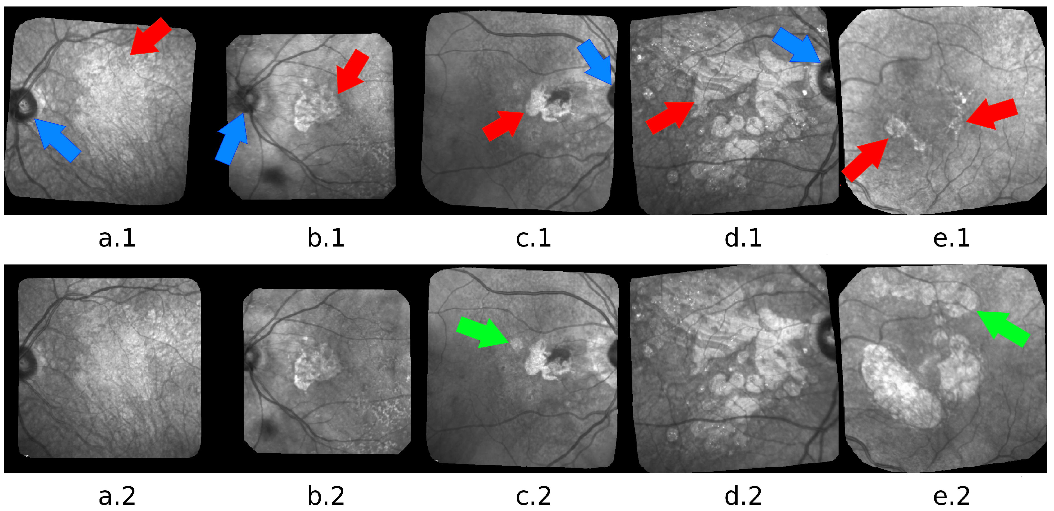
In this paper, we focus on the dry form of this pathology which currently does not have any treatments. It is characterized by a progressive loss of pigment epithelium which engenders a lesion located in the macula, growing slowly and impeding more and more the patient central vision. The lesions, called geographic atrophy (GA), can be observed in eye fundus images. Figure 1 shows examples of confocal Scanning Laser Ophtalmoscopy (cSLO) images acquired in infrared (IR), a commonly used imaging technique for ARMD patients, where the GA appears as brighter areas.
Despite intensive biological research, the factors involved in progression are poorly known. Therefore, clinical studies are needed to characterize the disease and its evolution. This can be done from eye fundus images, which are routinely acquired during the medical follow-up of patients. However, there are at present no efficient algorithms to automatically process large databases of images, even though it is very costly to process them manually: first, the manual delineation of the lesions is a very difficult and time-consuming task, given the complex structure of the GA. Secondly, the reliability of manual delineations is also an issue as even experts tends to disagree on their segmentations [1]. To solve this problem, in this work, we propose the first fully unsupervised application of automatic segmentation of GA using W-net [2] on cSLO IR acquired images (Section 2) and to assess how well it performs compared with other state of the art unsupervised methods. Our contribution is therefore three-fold:
- First, we propose a successful adaptation of the original developed by Xia et al. [2]. We modified the architecture to adapt it to our images and their specifics. In addition, furthermore, we fully trained our network and did not use any pre-trained model.
- Second, we propose the first realistic unsupervised approach to the very difficult problem of ARMD lesion segmentation. Indeed, this problem is already difficult for humans, and has very little labelled data (hence why we cannot use supervised neural networks), thus making it quite a challenging problem for unsupervised algorithms. In this regard, we achieve very decent performance considering the nature of the problem and the challenges it presents.
- Third, we propose a fair and extensive comparison with other unsupervised methods (neural networks and others) used in other fields that we have also adapted to tackle the same problem.
The remainder of this paper is organized as follows: Our method is presented in Section 4.1 and the compared methods in Section 4.2, after the description of our dataset (Section 2) and the related works (Section 3). The experimental results are shown in Section 5. In addition, finally, conclusions and insights as to our future works are discussed in Section 6.
2. Materials
We work on cSLO images acquired in IR. This modality is more robust and less invasive than fundus autofluorescence (FAF), and it has higher resolution and higher contrast between normal and diseased areas than color imaging, an older technology. Our database is composed of 18 series of images (328 images in total), showing the progression of the GA over several years for 13 patients (ARMD can affect both eyes). The time interval between two exams is about 6 months. All these images has been obtained from the Clinical Imaging Center of the Quinze-Vingts Hospital and all patients gave their informed consent for the use of images for clinical studies.
All images are in gray-levels (1 channel). Black borders are present because of the spatial registration process. Moreover, the images present illumination artifacts, blur and a non-uniform illumination. We preprocess jointly the images of every series as follows: we crop the images to suppress the black borders and resize them to 256 × 256 pixels; then we apply a joint correction of the overall illumination [3] so that any two processed images have comparable gray-levels. This algorithm does not completely compensate for uneven illumination, but the remaining defect is the same in all processed images, helping the ophthalmologists in the visual comparison of any two exams. From the segmentation point of view, the algorithm homogenizes the luminosity and the contrast of the images applied to the W-net and thus reduces the radiometric variability.
The major challenge of the segmentation task is to adapt to the large and complex variability of GA structures and to cope with all kinds of image defects. Figure 1 illustrates the difficulty: variability in size, shape, texture, number of GA areas, with new lesions that may appear at any time or merge; low contrast, blur, high ambiguity in the actual position of the border even for the most contrasted images. Please note that 18 series of images may not be enough to fully represent the real variability of GAs, and can lead to a lack of generality for deep learning-based methods.
In order to evaluate our algorithm, we asked ophthalmologists to delineate the GA areas. However, even with expert skills, the produced annotations may not be 100% reliable. Thus, the resulting pixel-wise annotations are only used to calculate classic segmentation quality measures (see Section 5.1).
3. Related Work
A lot of research has been done to propose segmentation algorithms of the GA. Standard algorithms have been applied, such as region growing [4,5] or active contour [6], region oriented variational methods with level set implementation [7,8], texture analysis [9] and watershed segmentation [10,11]. Most of the proposed methods are based on supervised machine learning approaches, with statistical models [12], random forests [13], random forests combined with Support Vector Machine [14] or k-nearest neighbor classifiers [15]. However, even in a supervised context, it is intricate to obtain a fully automatic algorithm reaching the required level of performance and some authors add human interaction to guide their algorithm [16,17]
Using deep learning, a reference model achieving impressive results for supervised segmentation is the U-net [18], and it has been implemented in many medical image segmentation problems (e.g., [19,20]). The U-net takes advantage of residual connections combined with a contracting and an expansive part. The authors of [21] proposed a supervised algorithm to follow-up the GA progression, using U-nets to first segment vessels and the optic disc, reducing the region of interest for the GA detection and then tracking it using intensity ratio between neighbor pixels. Other supervised deep learning-based methods were applied on ARMD as in [22] where they exploit transfer learning with deep neural networks to detect ARMD.
Last but not least, a segmentation task has been investigated in a scene parsing context. The authors of [23,24] exploit spatial pyramid pooling architecture in order to perform semantic segmentation between multiples objects present in a scene. However, as the U-Net, both PSP-Net and APSP-Net are deep supervised methods and their training requires a large amount of annotated data, which is not suitable for our application, as mentioned previously.
Thus, unsupervised methods can solve both the problem of data availability and the issue of the reliability of experts’ annotations. Unsupervised automatic segmentation is mainly handled in two steps: extracting features and then applying a clustering algorithm. The authors of [25] applied fuzzy CMeans clustering, which reached good performance for high-contrast FAF images, but performed less well for other modalities.
Using deep learning, the authors of [26] applied a joint auto-encoder (initially applied on satellite images [27]) on the same dataset we are using in this paper (see Section 2), in order to perform automatic change detection in an unsupervised context learning. The algorithm outperformed the state-of-the-art; however, as this model aims to detect changes, it is not comparable with automatic segmentation algorithm.
Kanezaki [28] combined clustering algorithm and CNN for a fully unsupervised model using a superpixel refinement method and achieving promising results for unsupervised automatic semantic segmentation. For a given image, the CNN first oversegments it (high number of cluster initially), then at each iteration, tries to reduce the number of cluster by merging them according to the result of the clustering algorithm.
Table 1 summarizes the pros and cons for the related works. As we want to exploit the dataset provided by the Clinical Imaging Center of the Quinze-Vingts Hospital (Section 2), which represent a non-invasive modality acquisition adapted to the patient follow-up, other modality use (which can engender better results due to a better quality of imaging) will be considered as a drawback. Supervised training is also considered a weakness because of the annotations reliability.
In this paper, we focus on unsupervised algorithms to segment the GA in IR cSLO eye fundus images with dry-ARMD. We propose to adapt the W-net [2] as well as three other unsupervised methods and compare them in an experimental study.
4. Methods
4.1. Our Method: W-Nets Adapted to ARMD Lesions Segmentation
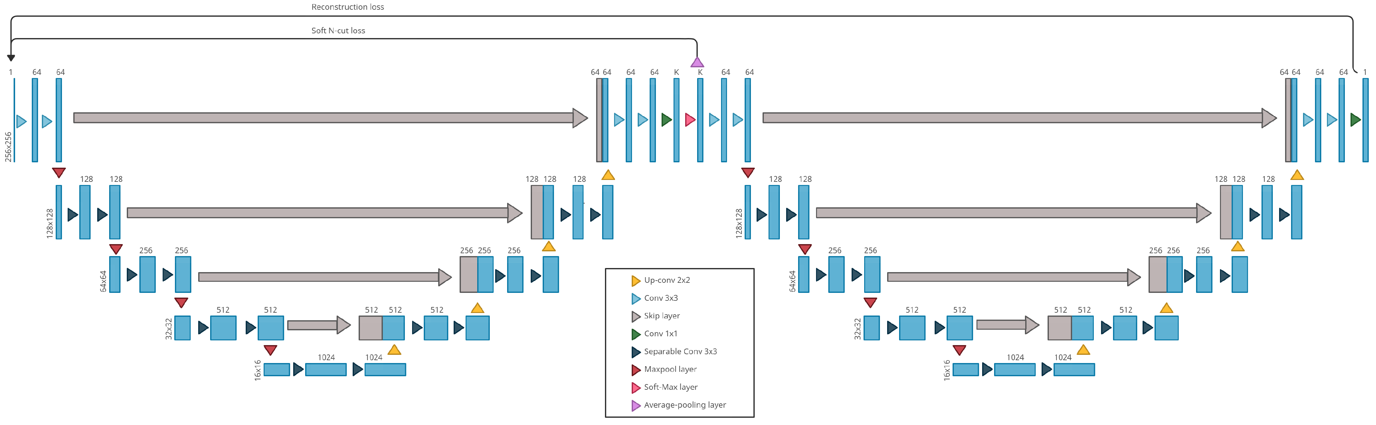
The W-net model is a fully convolutional autoencoder for which both encoder and decoder are U-net networks [18]. While U-nets are supervised neural networks commonly used for image segmentation, W-nets are the unsupervised equivalent. Unlike U-Nets, W-nets are trained using two loss functions. The first one is the usual reconstruction error used to train classic autoencoder, the second one is the soft-N-cut loss [2], a smooth version of the N-cut loss [29]. Minimizing the soft N-cut loss has the effect of enhancing the segmentation quality by maximizing the dissimilarity between the different clusters. The dissimilarity calculated is a function of the intensity pixel and the spatial position of the pixels.
During each training step, we have two successive optimization steps after each forward. First the full W-net is updated by back-propagating the self-reconstruction error (, where n is the number of pixel in the image), then only the encoding part is updated based on the soft N-cut loss :
with the probability for the pixel u to belong to the class k, and w a function which compute a weight for each couple of pixel, based on their position in the image and their intensity [29].
The architecture of our W-net is presented in Figure 2. Hence, the entire training of the W-net is unsupervised: the MSE loss is computed with the W-net output and the image input, while the soft-N-cut loss is computed with the probability map produced by the encoder (after the softmax layer in Figure 2) and the weights (which only need the image input to be computed). Compared with the original one, an average-pooling layer has been added before the computation of the soft N-cut loss. This loss is based on graph calculation, and thus, is memory-consuming when using large size images and not applicable on 256 × 256 sized images. Hence, the value of the soft N-cut loss is approximated by the value of the loss applied on the 128 × 128 (average) pooled input.
Once it has been trained on a set of unlabeled images, our network can be used on any ARMD cSLO images acquired in IR that have a similar resolution: For each pixel, the network will provide the probability of belonging to each class. Then applying a simple argmax will produce a segmentation. In our case, the purpose is to obtain two classes corresponding to the GA and the retina background. Thus, when the W-net is set with , one segmentation class will represent the GA and the other one the retina background. However, when the W-net is set with , we have to map the extra classes to the GA class or the background class. Finally, once trained, our W-net will always produce the same semantic classes for every image it processes, thus requiring a manual mapping only once.
4.2. Compared Methods
In this subsection, we present the three other compared algorithm: Gabor filters with KMeans [30], an active contour based model [5] and a model that combine CNN and clustering [28].
4.2.1. Gabor + KMeans
This algorithm is divided in three steps: creation of a set of Gabor filters, feature extraction using previous filters, pixels classification with KMeans on those features.
For a given frequency , Gabor function in spatial domain is a Gaussian modulated with a sinusoïd:
with and variances in direction x and y.
To capture features in multiple direction, we can add a rotation to the filter. Thus, we chose a set of directions, which define the set of Gabor filters. Each filter output pass through a non-linear function (sigmoïd function). The texture features are completed with spatial information (pixel position).
Finally, a KMeans clustering algorithm is applied on all the features, classifying each pixel and thus given us a pixel-wise segmentation.
4.2.2. Active Contour Model without Edges
Chan and Vese combined in [5] active contour methods, and Mumford-Shah functional and level set methods. Parametric active contour methods are based on a curve evolving technique: a parametrized curve evolve and is stopped using an edge detector, which usually rely on the gradient for a given image I. Such a method can then only detect objects with high gradient on their edges. Thus, the authors of [5] proposed a region oriented approach based on Mumford-Shah energy functional.
Let C be the evolving curve, I a given image, and the average value of I respectively inside C and outside C (case example with one object to detect from the background). The fitting energy function is defined as:
Thus, the solution of gives the boundary of the object we want to detect.
This algorithm is suitable for the GA segmentation as it can handle changes in topology with respect to the initialization, thanks to the level-set resolution method, as well as low contrast along the edges.
4.2.3. CNN + Superpixel Refinement
Kanezaki investigate the use of CNN for unsupervised segmentation. The algorithm is based on three assumptions:
- “Pixels of similar features are desired to be assigned the same label”
- “Spatially continuous pixels are desired to be assigned the same label”
- “The number of unique cluster labels is desired to be large”
For a given pixel of an RGB image (three channels) that we want to segment into q classes, we first extract p-dimensional features with p filters of size . Applying a linear classifier with weights and bias gives us a response map for each pixel: . Finally the cluster for each pixel is obtained by selecting the dimension with the greatest value. Thus, the output model is consistent with the features similarity constraint.
To satisfy the spatial continuity constraint, K fine superpixels are extracted and all the pixels of a given superpixel is forced to have the same cluster (which will be the most frequent cluster in the superpixel). Slic algorithm (KMeans-based segmentation algorithm) is used to compute the superpixels. Hence, the K classes obtained with Slic algorithm applied on the image I will correspond to the K superpixels.
The method in [28] aim to segment natural images (experiments on Berkeley Segmentation Dataset and Benchmark BSDS500) therefore, we do not have any prior knowledge of the number of unique clusters present in a given image. In this context, the algorithm must be able to output a variable number of clusters. Kanezaki’s strategy is to constraint the number of output clusters with a maximum number of cluster q. One has and to avoid the naive solution , he introduced the last constraint: q is preferred to be large. This is done by adding a whitening process, which transforms the response map into where each axis has zero mean and unit variance.
Two steps are applied alternatively to train the network:
- forward process: prediction of clusters with the network and refined cluster with the superpixel refinement process
- backward process: backpropagation of the signal error (cross-entropy loss) between the network response and the refined cluster
The training process of this model is different from the W-net one. One has to initialize and train the model for each individual image at contrary to the W-net which has to be trained only once. Indeed, the training process corresponds to the refinement of the model on a given image and can not be used to infer an other image.
5. Results
5.1. Experimental Setting
In our experiments, we use 18 series of 5 to 52 images (328 images). Due to the relatively small number of series and their variable size, we could not use k-folds validation. However, we used 8 different random combinations of 12 series to train the model and 6 for the tests. Our W-net is compared with Gabor Filters for texture extraction [30] and KMeans algorithm for the segmentation, the CNN model with superpixel refinement [28] and finally an active contour model [5].
As the lesions can only grow bigger, we also try to see if adding the segmentation from the previous image improves the results or not: we merge the segmentation provided by our W-net for the current Image with the segmentation of the same W-net for the previous image . This modification is supposed to reduce the risk of undersegmentation.
Our network is set with a kernel size of 3, and each U-net produces 1024 features after the contracting part. Our model is trained on 250 epochs, using two Adam optimizers. The number of classes is set to 3 in the experiments: using two classes, the latent representation is too restrictive. Using three classes, the network learns extra classes for the background (healthy regions and blood vessels) or the ARMD lesions.
Hyperparameters for Gabor filters methods, Chan and Vese’s method, and Kanezaki’s method have been tuned manually by referring to the visual output. Therefore, the fixed parameters are not the optimal ones, but a compromise to obtain the best average output.
The evaluation is based on the pixels’ classification using true positive (TP), false positive (FP), and false negative (FN) to build dice metrics such as the F1-Score:
with
and
KMeans algorithm output directly the classification an not the probability to belong to each class. However, those probabilities are needed to compute the ROC curve. Hence we use fuzzy CMeans instead (which provides, with an argmax, the same output as Kmeans)
All the experiments have been done using a GEFORCE RTX 3090 GPU with 24Gb of RAM, Python 3.8.5, Pytorch 1.7.1 and Cuda 11.1.
5.2. Experimental Results
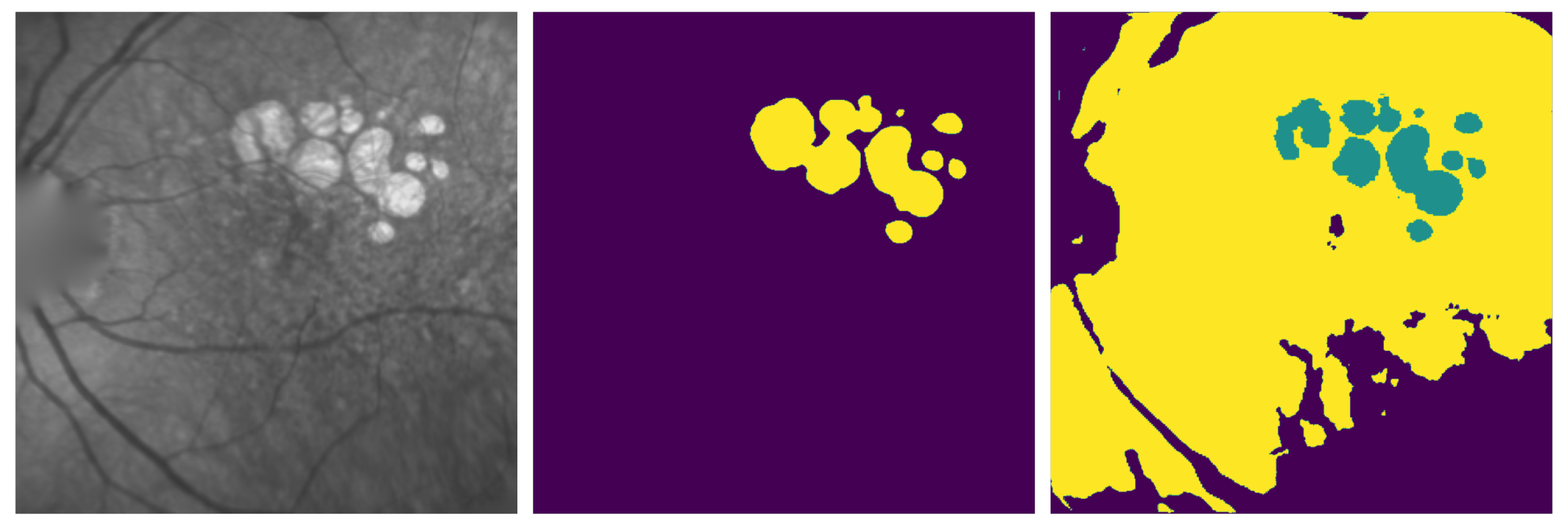
As explained before, our W-net is set to three classes. With this configuration, we manually map the classes to the lesion or the background. Figure 3 shows an example of different classes obtained with our 3-class W-net: the class of interest corresponding to the GA is in green. The two other classes belong to the retina background. Please note that this mapping is arbitrary and may not be optimal in specific cases.
Table 2 shows the average dice score (F1), precision and recall on the training set (W-net is the only model that need to be trained), while Table 3 focuses on the test set and features the comparison with the other algorithms introduced in Section 5.1. As one can see, W-net is the most relevant method. It has the best F1 score and achieves higher quality results with a better precision and recall. Moreover, our W-net has a smaller standard deviation for the F1 score and the precision, resulting in a more stable model.
The bottom line (W-net + ) in both tables corresponds to the fusion of a given segmentation with the previous one (see Section 5.1). However, we can see that this modification does not lead to any significant increase in the result quality: while the Recall is indeed better (less under-segmentation), the F1 score is not significantly different from the one of our method on individual images. This can be explained by an accumulation of over-segmented areas propagating through the series, which is confirmed by a worst Precision that we observe.
In any case, we can see that except for the recall—which can be explained by cases of under-segmentation—our W-net approaches outperform the Gabor filter and KMeans approach, Active contour method, and CNN model with superpixel refinement.
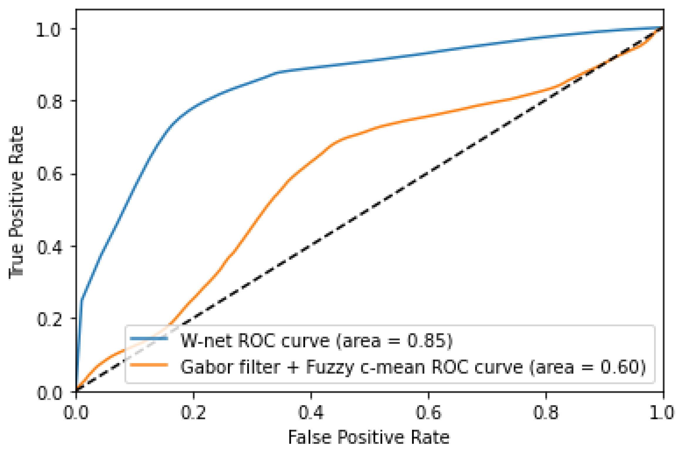
Our W-net superiority is also shown in Figure 4, where we can clearly see that the W-net is nearer to the perfect model compared to the Gabor filter with Fuzzy CMeans method. Please note that we compared the ROC curve for the two most relevant algorithm according to the results in Table 2 and Table 3.
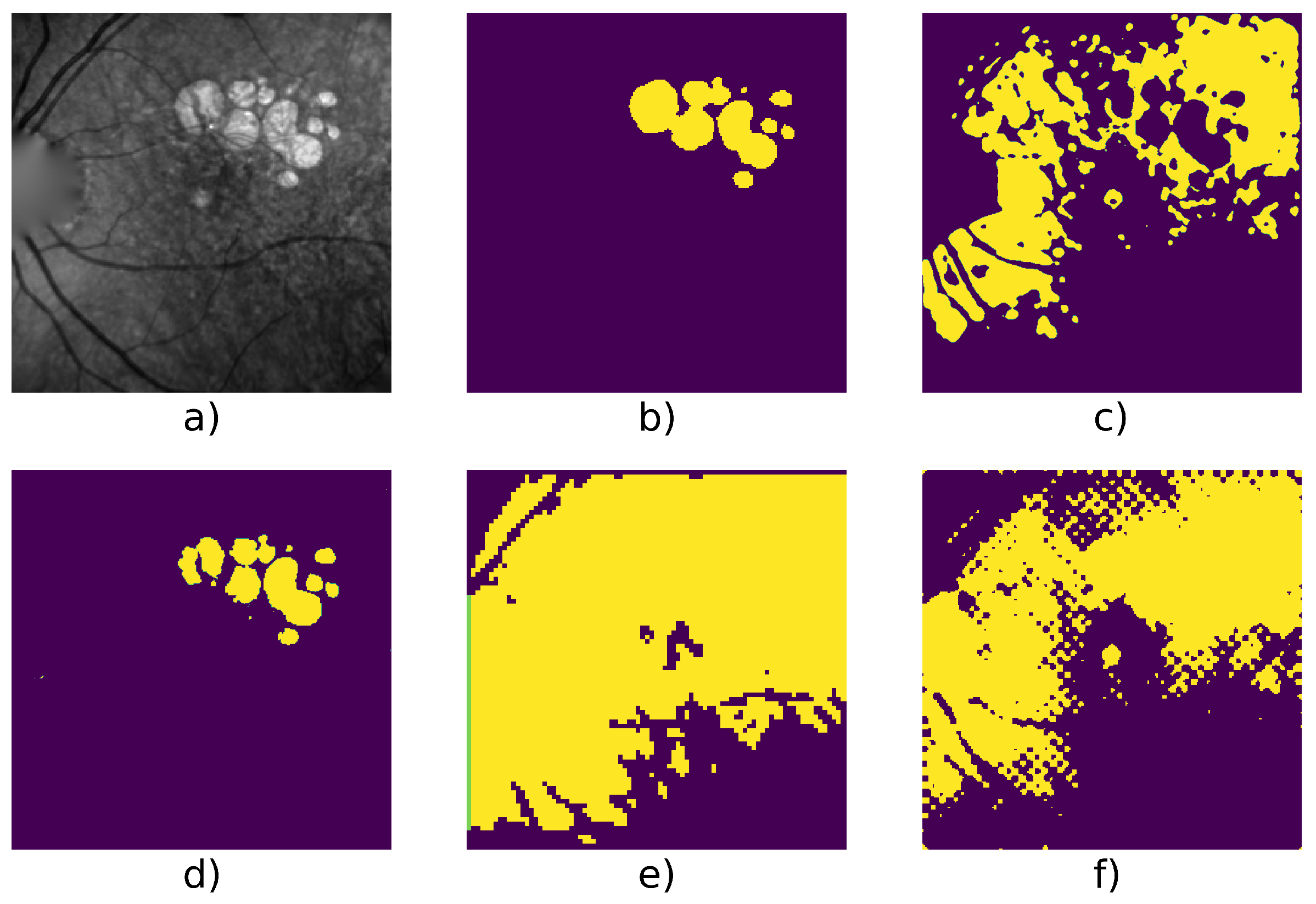
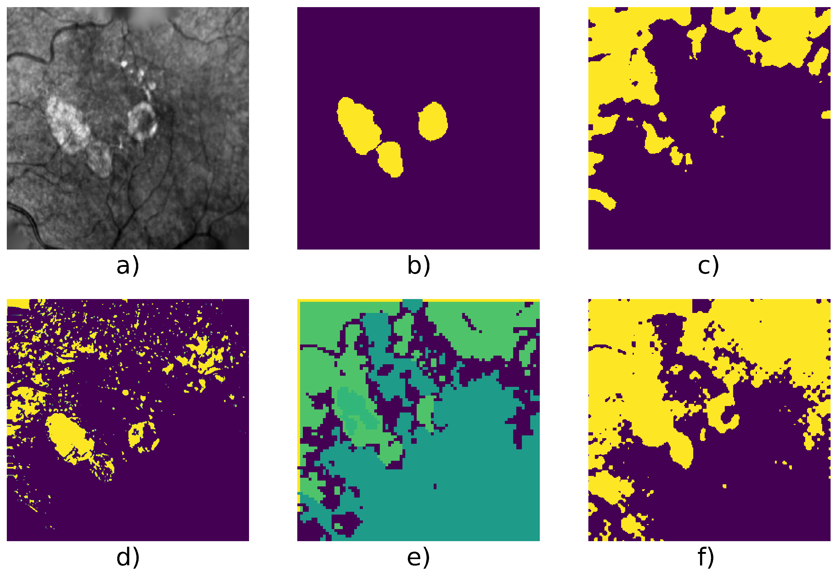
Table 4 shows detailed score on 6 series and we can see an example taken from each series in Figure 5, Figure 6, Figure 7, Figure 8, Figure 9 and Figure 10.
Figure 5 and Figure 9 show examples from average cases (in terms of complexity of the lesion’s structures), where W-net outperforms other methods with a mean F1 score on the series of 0.98 for the first series, and 0.946 for the second one. This also highlights the capacity of W-net to correlate the different classes based on intensity values, while the other methods attempt (and fails) to do so based on textures rather than intensity.
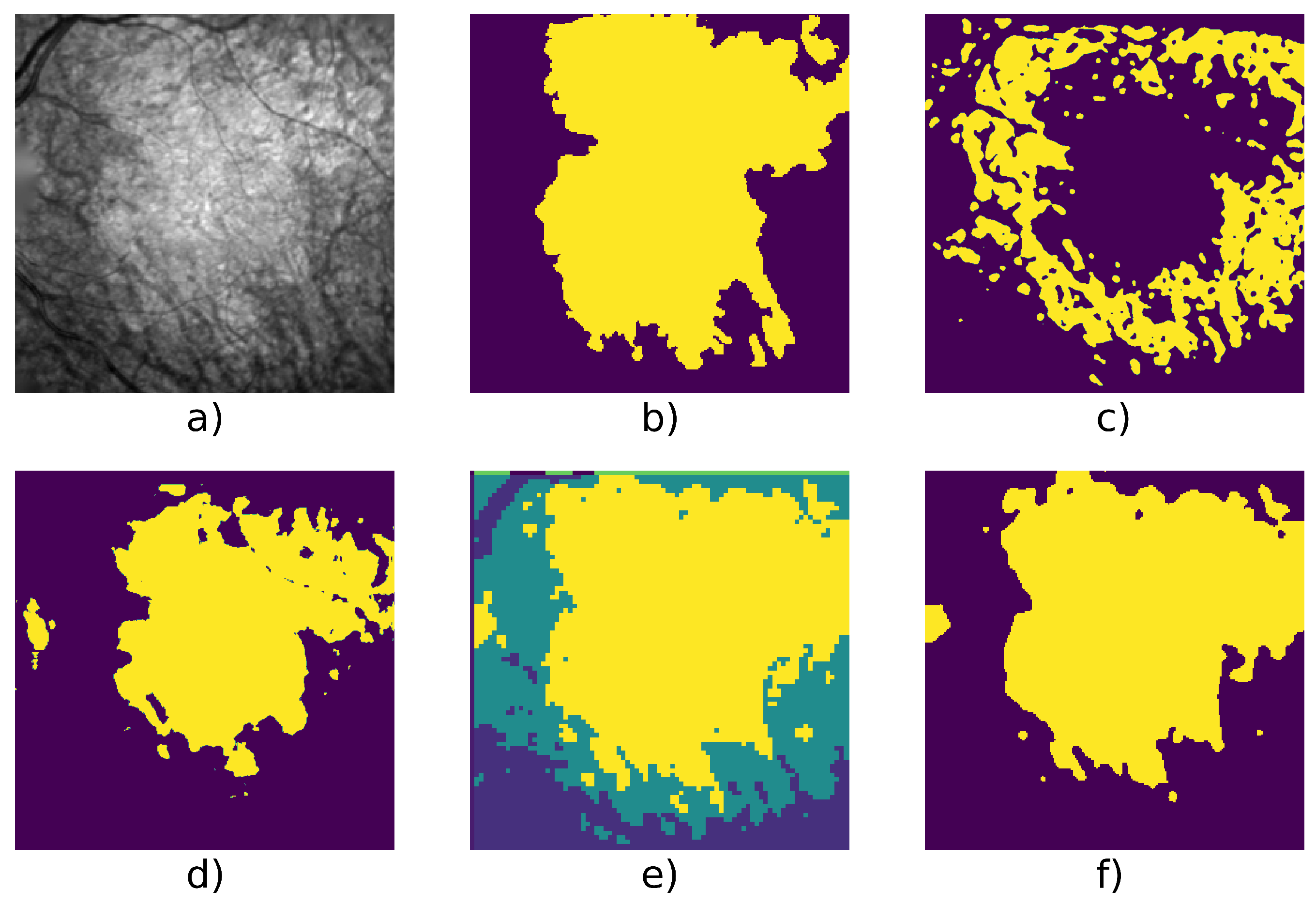
As said in the introduction, a lesion with blurred outlines will be difficult to segment. This is illustrated in Figure 6 where the Gabor filter algorithm fails to segment the GA, while the W-net does better but with some undersegmentation. In this case, CNN with super-pixel refinement method and the active contour methods output a better result; however, the first one gives more classes than expected due to the algorithm’s setting [28].
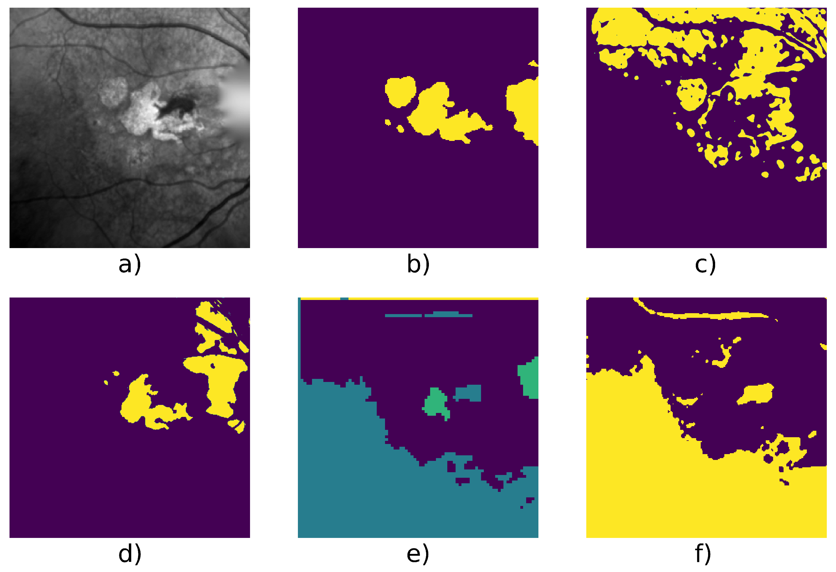
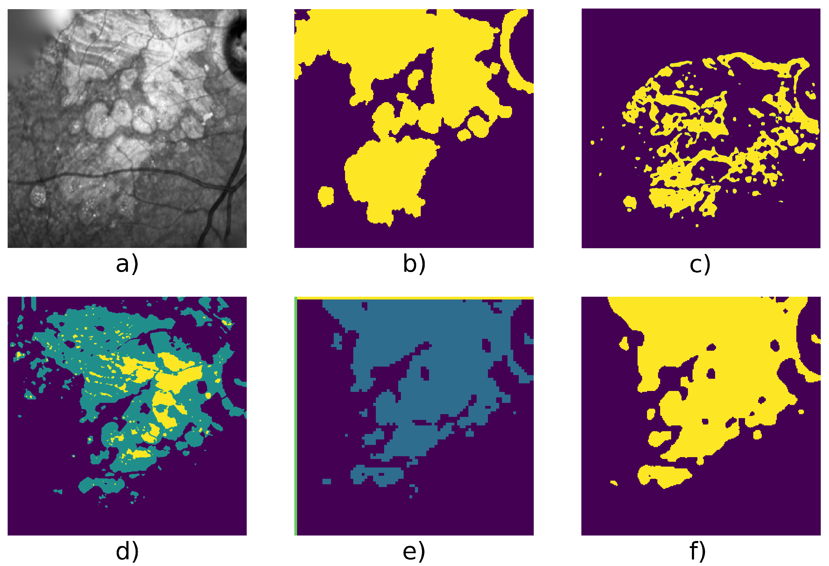
Finally, Figure 7 and Figure 10 show two cases where the lesion has different levels of contrast. These are good examples of cases in which it is useful to have three classes (which are represented in yellow/green/purple for example d): as one can see, most of the lesion class is contained within the green class, which is one of the two retina background classes, while the yellow class is the GA class (according to our mapping). In those cases and without the manual cluster/class mapping, both Gabor method and our W-net would fail to identify the GA. The W-net reliance on intensity creates this undersegmentation risk: a low-intensity region is more likely to belong to the background retina class. However, because of the extra class, in the case of our method, the segmentation can still easily be manually fixed. In this case, Kanezaki’s method and Chan and Vese’s method provide a better quality results. Nevertheless, it highlights the limits of unsupervised methods where user intervention is sometimes inevitable.
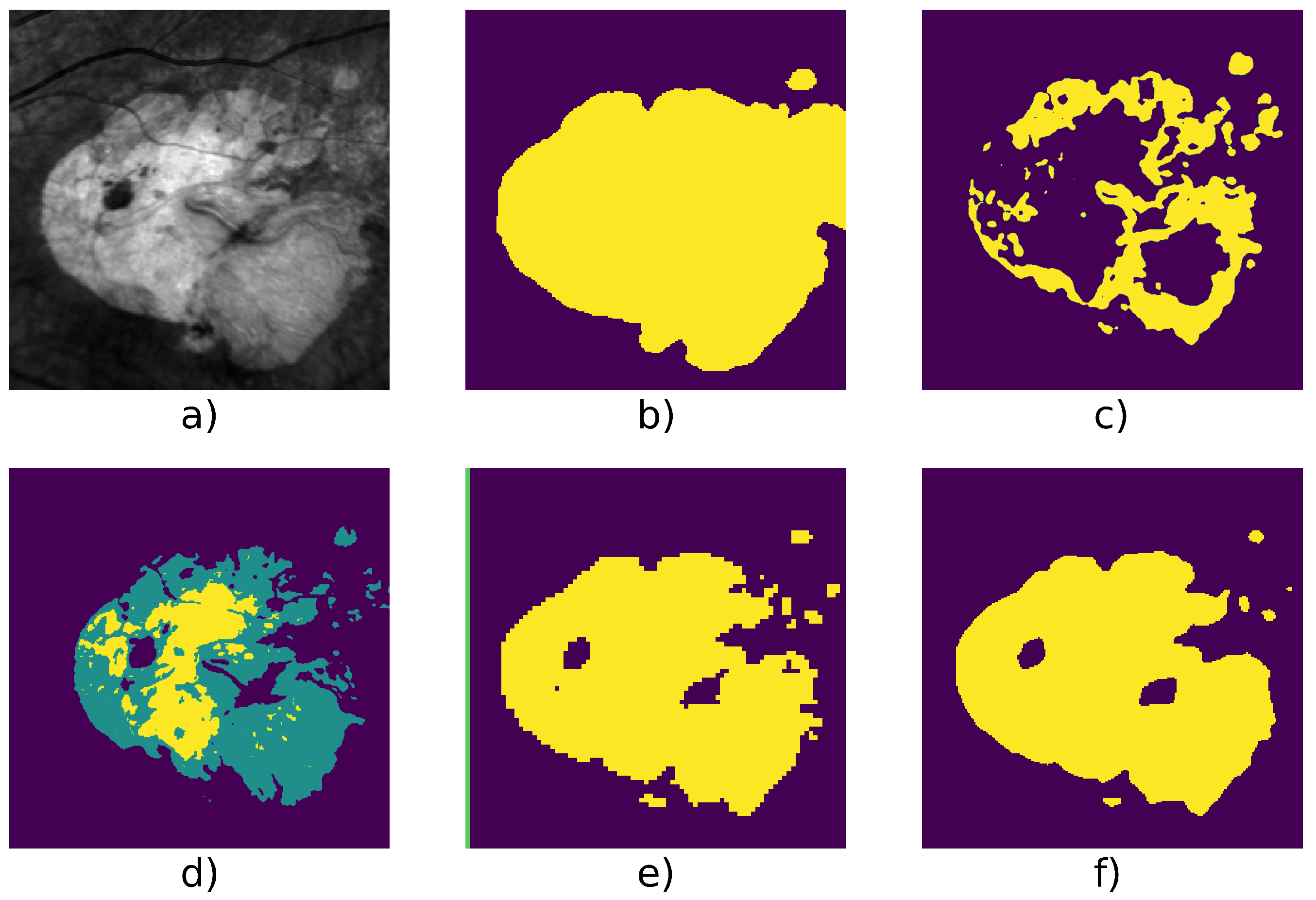
We can also mention that W-net outperfoms other compared algorithm on a long serie (Patient Id 020, fourth line of Table 4, Figure 9) which contain 50 images. This serie is an example of ARMD progression: as we can see in Figure 1e, the ARMD lesions progress from two tiny GA to three consequent GA in 6 years. Images from the beginning of the serie thus contain small GA which enhances risk of oversegmentation. This can also be seen in Figure 8 where despite a higher quality result provided by our W-net, it did not detect a small GA and oversegmented the top right region of the image.
From these experiments, we can see that in most cases, our modified W-net produces a better quality segmentation than the other algorithms and has the advantage to be more stable. Furthermore, from cases such as Figure 6, we can see that because of its reliance on textures only, the Gabor filter based approach sometimes entirely fails to capture the GA and appears to detect only peripheral areas of textural transition. However, our proposed W-net -despite some mismatches between the clusters and the classes- manages to have a group of clusters that match the GA class. The CNN with superpixel refinement method provides relevant outputs but need a post-processing step to enhance the segmentation quality. In fact, the results are not smooth enough, and we have no guarantee to obtain two final clusters: the number of clusters in the outuput can vary from an image to another (even for two successive images from a given serie). This is due to the third criterion of Kanezaki’s system: the segmentation context is different from ours, we aim to segment a fixed number of classes. Last but not least, active contour methods can produce a better quality result in some specific cases as they can totally fail in an average case. That highlight the lack of generality of those methods compared to the high variability of both texture and structure of the GA regions.
6. Conclusions and Future Works
The automatic segmentation of dry-ARMD lesion is a difficult problem with significant implications for patients afflicted by this disease, as it may allow for a better monitoring of the lesions progression. Despite the complexity of the task, we proposed a promising adaptation of W-nets to this problem. Our algorithm is fully unsupervised, which makes it possible to achieve good quality results without any need for labeled data that are difficult to come by, as even expert ophthalmologists often disagree on the proper segmentation of the lesions for difficult cases.
Our proposed algorithm was tested on 328 images from 18 patients, and has proven to be very effective. However, we identified a weakness, which is the W-net’s tendency to undersegment the lesions. This can be explained by the intensity distribution in the images: a single-channel input model can only exploit pixel intensity and spatial information. Thus, high intensity regions will generally correspond to be a part of a lesion, while low intensity regions generally correspond to be a part of the background. However, there is a high variability in the contrast in the images and some cases can show a GA with an intensity barely lighter than the background, hence the interest of having three classes. Furthermore, the most difficult case for this task is when the lesion has a blurred outline (e.g., Figure 1(a.1)). Automatic unsupervised segmentation algorithms tend to fail in this specific case in two different ways: if the blurry lesion is too small, the result will be over-segmented. If the blurry lesion is too large, the result will be under-segmented.
On the other side, the three other algorithms have a lack of generality because of the restrictive settings. To better exploit their advantage, a proper fine tuning in each specific case should be needed, leading to a supervised process that requires medical expertise.
Because of the reliability of the ground truths and the cost to produce them, the unsupervised context is the most appropriate to face this issue
In our future work, we plan on improving our segmentation capabilities by combining our proposed algorithm with generative adversarial networks [31] that have been shown to produce higher quality outputs and to outperform traditional convolutional autoencoders. Thus, a first improvement of the W-net is an adversial training, which could improve the reconstruction quality and therefore the segmentation map quality.
Finally, deep learning performance depends a lot on the dataset training, thus enrich the dataset with more series and with data augmentation can enhance robustness and performance.
Author Contributions
M.P. is with the Clinical Imaging Center of Paris Quinze-Vingts hospital and provided the data after a first preprocessing step. M.P. also provided the medical knowledge necessary to interpret our algorithm’s results. F.R. and M.P. worked together to produce and validate ground truths as reliable as possible. F.R. worked on data curation and the preprocessing algorithm for lighting correction. Most of the software programming, investigation, and experiments, as well as the result visualization were done by C.R. during his internship and his 1st year of PhD thesis. J.S. and F.R. worked on the problem analysis and conceptualization, as well as the experiment design and validation. C.R., F.R. and J.S. all participated in the redaction and proof-reading of the manuscript. F.R., M.P. and J.S. conducted the project and are C.R. Ph.D. advisors. All authors have read and agreed to the published version of the manuscript.
Funding
This research is partially funded by Sorbonne University, EDITE PhD scholarship.
Informed Consent Statement
This study has been approved by a French ethical committee (Comité de Protection des Personnes) and all participants gave informed consent.
Data Availability Statement
Sample images and the source code are available in https://github.com/clement-royer/Unsupervised-segmentation-of-dry-ARMD-lesions-in-cSLO-images-using-W-nets (accessed on 25 June 2021). Please note that since we are dealing with medical images, we are only allowed to disclose a limited number of them and not the full time series.
Conflicts of Interest
The authors declare no conflict of interest.
Abbreviations
The following abbreviations are used in this manuscript:
| AE | Autoencoder |
| APSP | Atrous Pyramid Spatial Pooling |
| ARMD or AMD | Age-Related Macular Degeneration |
| CNN | Convolutional Neural Networks |
| cSLO | confocal Scanning Laser Ophthalmoscopy |
| FAF | Fundus Autofluorescence |
| GA | Geographic Atrophy |
| IR | Infrared |
| OCT | Optical Coherence Tomography |
| PSP | Pyramid Spatial Pooling |
References
- Platanios, E.A.; Al-Shedivat, M.; Xing, E.; Mitchell, T. Learning from Imperfect Annotations: An End-to-End Approach. 2020. Available online: https://openreview.net/forum?id=rJlVdREKDS (accessed on 25 June 2021).
- Xia, X.; Kulis, B. W-Net: A Deep Model for Fully Unsupervised Image Segmentation. arXiv 2017, arXiv:1711.08506. [Google Scholar]
- Rossant, F.; Paques, M. Normalization of series of fundus images to monitor the geographic atrophy growth in dry age-related macular degeneration. Comput. Methods Programs Biomed. 2021, 208, 106234. [Google Scholar] [CrossRef] [PubMed]
- Köse, C.; Sevik, U.; Gençalioglu, O. Automatic segmentation of age-related macular degeneration in retinal fundus images. Comput. Biol. Med. 2008, 38, 611–619. [Google Scholar] [CrossRef] [PubMed]
- Chan, T.; Vese, L. Active contours without edges. IEEE Trans. Image Process. 2001, 10, 266–277. [Google Scholar] [CrossRef] [PubMed] [Green Version]
- Abdullah, A.S.; Rahebi, J.; Özok, Y.; Aljanabi, M. A new and effective method for human retina optic disc segmentation with fuzzy clustering method based on active contour model. Med. Biol. Eng. Comput. 2019, 58. [Google Scholar] [CrossRef]
- Hu, Z.; Medioni, G.; Hernandez, M.; Hariri, A.; Wu, X.; Sadda, S. Segmentation of the Geographic Atrophy in Spectral-Domain Optical Coherence Tomography and Fundus Autofluorescence Images. Investig. Ophthalmol. Vis. Sci. 2013, 54, 8375–8383. [Google Scholar] [CrossRef] [PubMed] [Green Version]
- Lee, N.; Laine, A.; Smith, R. A hybrid segmentation approach for geographic atrophy in fundus auto-fluorescence images for diagnosis of age-related macular degeneration. In Proceedings of the 2007 29th Annual International Conference of the IEEE Engineering in Medicine and Biology Society, Lyon, France, 22–26 August 2007. [Google Scholar]
- Köse, C.; Sevik, U.; Gençalioğlu, O.; Ikibaş, C.; Kayikiçioğlu, T. A Statistical Segmentation Method for Measuring Age-Related Macular Degeneration in Retinal Fundus Images. J. Med. Syst. 2010, 34, 1–13. [Google Scholar] [CrossRef] [PubMed]
- Cousty, J.; Bertrand, G.; Najman, L.; Couprie, M. Watershed Cuts: Thinnings, Shortest Path Forests, and Topological Watersheds. IEEE Trans. Pattern Anal. Mach. Intell. 2010, 32, 925–939. [Google Scholar] [CrossRef] [PubMed] [Green Version]
- G N, G.; Kothari, A.; Rajan, J. Marker Controlled Watershed Transform for Intra-Retinal Cysts Segmentation from Optical Coherence Tomography B-Scans. Pattern Recognit. Lett. 2017, 139, 86–94. [Google Scholar] [CrossRef]
- Köse, C.; İkibaş, C. Statistical Techniques for Detection of Optic Disc and Macula and Parameters Measurement in Retinal Fundus Images. J. Med. Biol. Eng. 2011, 31, 395–404. [Google Scholar] [CrossRef]
- Feeny, A.K.; Tadarati, M.; Freund, D.E.; Bressler, N.M.; Burlina, P. Automated segmentation of geographic atrophy of the retinal epithelium via random forests in AREDS color fundus images. Comput. Biol. Med. 2015, 65, 124–136. [Google Scholar] [CrossRef] [PubMed] [Green Version]
- Phan, T.V.; Seoud, L.; Chakor, H.; Cheriet, F. Automatic Screening and Grading of Age-Related Macular Degeneration from Texture Analysis of Fundus Images. J. Ophthalmol. 2016, 2016, 5893601. [Google Scholar] [CrossRef] [PubMed] [Green Version]
- Hu, Z.; Medioni, G.; Hernandez, M.; Sadda, S. Automated segmentation of geographic atrophy in fundus autofluorescence images using supervised pixel classification. J. Med. Imaging 2014, 2, 014501. [Google Scholar] [CrossRef] [PubMed]
- Lee, N.; Smith, R.T.; Laine, A.F. Interactive segmentation for geographic atrophy in retinal fundus images. Conf. Rec. Conf. Signals Syst. Comput. 2008, 2008, 655–658. [Google Scholar] [CrossRef] [Green Version]
- Deckert, A.; Schmitz-Valckenberg, S.; Jorzik, J.; Bindewald, A.; Holz, F.; Mansmann, U. Automated analysis of digital fundus autofluorescence images of geographic atrophy in advanced age-related macular degeneration using confocal scanning laser ophthalmoscopy (cSLO). BMC Ophthalmol. 2005, 5, 8. [Google Scholar] [CrossRef] [PubMed] [Green Version]
- Ronneberger, O.; Fischer, P.; Brox, T. U-Net: Convolutional Networks for Biomedical Image Segmentation. In Proceedings of the Medical Image Computing and Computer-Assisted Intervention—MICCAI 2015—18th International Conference, Munich, Germany, 5–9 October 2015; pp. 234–241. [Google Scholar]
- Milletari, F.; Navab, N.; Ahmadi, S. V-Net: Fully Convolutional Neural Networks for Volumetric Medical Image Segmentation. In Proceedings of the Fourth International Conference on 3D Vision, 3DV 2016, Stanford, CA, USA, 25–28 October 2016; IEEE Computer Society: Washington, DC, USA, 2016; pp. 565–571. [Google Scholar] [CrossRef] [Green Version]
- Çiçek, Ö.; Abdulkadir, A.; Lienkamp, S.S.; Brox, T.; Ronneberger, O. 3D U-Net: Learning Dense Volumetric Segmentation from Sparse Annotation. In Proceedings of the Medical Image Computing and Computer-Assisted Intervention—MICCAI 2016—19th International Conference, Athens, Greece, 17–21 October 2016; pp. 424–432. [Google Scholar]
- Hussain, M.A.; Govindaiah, A.; Souied, E.; Smith, R.T.; Bhuiyan, A. Automated tracking and change detection for Age-related Macular Degeneration Progression using retinal fundus imaging. In Proceedings of the 2018 Joint 7th International Conference on Informatics, Electronics & Vision (ICIEV) and 2018 2nd International Conference on Imaging, Vision & Pattern Recognition (icIVPR), Kitakyushu, Japan, 25–29 June 2018; pp. 394–398. [Google Scholar] [CrossRef]
- Burlina, P.; Freund, D.E.; Joshi, N.; Wolfson, Y.; Bressler, N.M. Detection of age-related macular degeneration via deep learning. In Proceedings of the 2016 IEEE 13th International Symposium on Biomedical Imaging (ISBI), Prague, Czech Republic, 13–16 April 2016; pp. 184–188. [Google Scholar] [CrossRef]
- Zhao, H.; Shi, J.; Qi, X.; Wang, X.; Jia, J. Pyramid Scene Parsing Network. In Proceedings of the 2017 IEEE Conference on Computer Vision and Pattern Recognition (CVPR), Honolulu, HI, USA, 21–26 July 2017; pp. 6230–6239. [Google Scholar] [CrossRef] [Green Version]
- Chen, L.C.; Zhu, Y.; Papandreou, G.; Schroff, F.; Adam, H. Encoder-Decoder with Atrous Separable Convolution for Semantic Image Segmentation. In Proceedings of the European Conference on Computer Vision, Munich, Germany, 8–14 September 2018. [Google Scholar]
- Ramsey, D.J.; Sunness, J.S.; Malviya, P.; Applegate, C.; Hager, G.D.; Handa, J.T. Automated image alignment and segmentation to follow progression of geographic atrophy in age-related macular degeneration. Retina 2014, 34, 1296–1307. [Google Scholar] [CrossRef] [PubMed]
- Dupont, G.; Kalinicheva, E.; Sublime, J.; Rossant, F.; Pâques, M. Analyzing Age-Related Macular Degeneration Progression in Patients with Geographic Atrophy Using Joint Autoencoders for Unsupervised Change Detection. J. Imaging 2020, 6, 57. [Google Scholar] [CrossRef]
- Kalinicheva, E.; Sublime, J.; Trocan, M. Change Detection in Satellite Images using Reconstruction Errors of Joint Autoencoders. In Artificial Neural Networks and Machine Learning—ICANN 2019: Image Processing; Springer: Munich, Germany, 2019; pp. 637–648. [Google Scholar] [CrossRef]
- Kanezaki, A. Unsupervised Image Segmentation by Backpropagation. In Proceedings of the IEEE International Conference on Acoustics, Speech, and Signal Processing (ICASSP), Calgary, AB, Canada, 15–20 April 2018. [Google Scholar]
- Tang, M.; Djelouah, A.; Perazzi, F.; Boykov, Y.; Schroers, C. Normalized Cut Loss for Weakly-Supervised CNN Segmentation. In Proceedings of the 2018 IEEE Conference on Computer Vision and Pattern Recognition, CVPR 2018, Salt Lake City, UT, USA, 18–22 June 2018. [Google Scholar] [CrossRef] [Green Version]
- Jain, A.; Farrokhnia, F. Unsupervised Texture Segmentation Using Gabor Filters. Pattern Recognit. 1990, 24, 14–19. [Google Scholar] [CrossRef] [Green Version]
- Goodfellow, I.J.; Pouget-Abadie, J.; Mirza, M.; Xu, B.; Warde-Farley, D.; Ozair, S.; Courville, A.C.; Bengio, Y. Generative adversarial networks. Commun. ACM 2020, 63, 139–144. [Google Scholar] [CrossRef]
Figure 1.
Five pairs of images: (a) advanced case with blur, low contrast and very indented GA boundary; (b) less advanced case with lesions at the center and around the optic disk; (c) a new lesion appears in the second image (green arrow); (d) GA with complex structure and texture; (e) example of progression of a GA during 6 years. A third GA appeared (green arrow). Arrows point to the GA (red) and to the optic disk (blue).

Figure 2.
Our W-net architecture for ARMD lesions segmentation.

Figure 3.
Example of three classes W-net output. From left to right: original image, ground truth, 3-class W-net output.
Figure 3.
Example of three classes W-net output. From left to right: original image, ground truth, 3-class W-net output.

Figure 4.
Receiver Operating Characteristic curve of Gabor filter + fuzzy CMeans and W-net.

Figure 5.
Patient id 117: (a) original image, (b) ground truth, (c) Gabor method segmentation, (d) W-net segmentation, (e) CNN + superpixel refinement segmentation, (f) active contour segmentation.
Figure 5.
Patient id 117: (a) original image, (b) ground truth, (c) Gabor method segmentation, (d) W-net segmentation, (e) CNN + superpixel refinement segmentation, (f) active contour segmentation.

Figure 6.
Patient id 005: (a) original image, (b) ground truth, (c) Gabor method segmentation, (d) W-net segmentation, (e) CNN + superpixel refinement segmentation, (f) active contour segmentation.
Figure 6.
Patient id 005: (a) original image, (b) ground truth, (c) Gabor method segmentation, (d) W-net segmentation, (e) CNN + superpixel refinement segmentation, (f) active contour segmentation.

Figure 7.
Patient id 016: (a) original image, (b) ground truth, (c) Gabor method segmentation, (d) W-net clusters, (e) CNN + superpixel refinement segmentation, (f) active contour segmentation.
Figure 7.
Patient id 016: (a) original image, (b) ground truth, (c) Gabor method segmentation, (d) W-net clusters, (e) CNN + superpixel refinement segmentation, (f) active contour segmentation.

Figure 8.
Patient id 010: (a) original image, (b) ground truth, (c) Gabor method segmentation, (d) W-net segmentation, (e) CNN + superpixel refinement segmentation, (f) active contour segmentation.
Figure 8.
Patient id 010: (a) original image, (b) ground truth, (c) Gabor method segmentation, (d) W-net segmentation, (e) CNN + superpixel refinement segmentation, (f) active contour segmentation.

Figure 9.
Patient id 020: (a) original image, (b) ground truth, (c) Gabor method segmentation, (d) W-net segmentation, (e) CNN + superpixel refinement segmentation, (f) active contour segmentation.
Figure 9.
Patient id 020: (a) original image, (b) ground truth, (c) Gabor method segmentation, (d) W-net segmentation, (e) CNN + superpixel refinement segmentation, (f) active contour segmentation.

Figure 10.
Patient id 109: (a) original image, (b) ground truth, (c) Gabor method segmentation, (d) W-net clusters, (e) CNN + superpixel refinement segmentation, (f) active contour segmentation.
Figure 10.
Patient id 109: (a) original image, (b) ground truth, (c) Gabor method segmentation, (d) W-net clusters, (e) CNN + superpixel refinement segmentation, (f) active contour segmentation.


Table 1.
Comparative summary of related works.
| Method | Pros | Cons | |
|---|---|---|---|
| Region oriented [4,5] | High performance on ARMD, semi-supervised (seeds) | FAF/OCT images | Conventionnal methods |
| Active contour [5,6] | High performance on retinal cases | Segment optic discs | |
| Statistical [12] | High performance on retinal cases | Segment blood vessels and optic discs | |
| Random Forest [13] | High performance on ARMD | Color fundus images, supervised | |
| Random Forest + SVM [14] | High performance on ARMD | Screening and grading task, supervised | |
| Fuzzy C-means [25] | Unsupervised, high performance on ARMD | High contrast FAF images | |
| K-NN [15] | High performance on ARMD | FAF images, supervised | |
| Watershed [10,11] | Semi supervised (seeds) | OCT images | |
| U-net [18,21] | High performance on ARMD | Supervised, training on GPU | Deep learning methods |
| Transfert learning on ARMD [22] | High performance | Supervised, color fundus images | |
| Scene parsing [23,24] | High performance | Supervised, requires multiple objects in a scene, training on GPU | |
| Change detection [26] | Unsupervised, applied on the same dataset | Change detection task | |
| CNN + Superpixel refinement [28] | Unsupervised, no training | Produce a variable number of cluster in the segmentation | |
| W-net [2] | Unsupervised, robust | Training on GPU | |
| Our W-net | Unsupervised, fast inference use, robust, high performance on ARMD | Training on GPU | |
| Human interaction [16,17] | High performance on ARMD | Require human interaction | Other methods |
Table 2.
Average W-net dice scores on the training set.
| Method | F1 | Precision | Recall |
|---|---|---|---|
| W-net | 0.83 ± 0.09 | 0.87 ± 0.08 | 0.81 ± 0.13 |
| W-net + | 0.82 ± 0.07 | 0.82 ± 0.10 | 0.82 ± 0.11 |
Table 3.
Average dice scores on the test set.
| Method | F1 | Precision | Recall |
|---|---|---|---|
| Active contour (Chan & Vese [5]) | 0.73 ± 0.07 | 0.64 ± 0.13 | 0.86 ± 0.05 |
| CNN + Superpixel Refinement (Kanezaki [28]) | 0.65 ± 0.07 | 0.54 ± 0.10 | 0.85 ± 0.06 |
| Gabor + KMeans [30] | 0.77 ± 0.08 | 0.80 ± 0.12 | 0.75 ± 0.08 |
| Our W-net | 0.87 ± 0.07 | 0.90 ± 0.07 | 0.85 ± 0.11 |
| W-net + | 0.85 ± 0.06 | 0.84 ± 0.07 | 0.87 ± 0.09 |
Table 4.
Detailed dice scores on specific series.
| Patient Id | Method | F1 | Precision | Recall | Nb. of Images | Fig. |
|---|---|---|---|---|---|---|
| 005 | Active Contour | 0.787 | 0.779 | 0.795 | 9 | Figure 6 |
| CNN + Superpixel refinement | 0.690 | 0.623 | 0.787 | |||
| Gabor + KMeans | 0.791 | 0.760 | 0.828 | |||
| Our W-net | 0.785 | 0.806 | 0.765 | |||
| W-net + | 0.799 | 0.805 | 0.792 | |||
| 010 | Active Contour | 0.644 | 0.504 | 0.892 | 6 | Figure 8 |
| CNN + Superpixel refinement | 0.589 | 0.440 | 0.909 | |||
| Gabor + KMeans | 0.809 | 0.907 | 0.731 | |||
| Our W-net | 0.922 | 0.921 | 0.922 | |||
| W-net + | 0.919 | 0.910 | 0.927 | |||
| 016 | Active Contour | 0.849 | 0.869 | 0.828 | 31 | Figure 7 |
| CNN + Superpixel refinement | 0.790 | 0.752 | 0.840 | |||
| Gabor + KMeans | 0.678 | 0.596 | 0.786 | |||
| Our W-net | 0.676 | 0.880 | 0.924 | |||
| W-net + | 0.706 | 0.817 | 0.622 | |||
| 020 | Active Contour | 0.654 | 0.516 | 0.901 | 50 | Figure 9 |
| CNN + Superpixel refinement | 0.622 | 0.489 | 0.898 | |||
| Gabor + KMeans | 0.744 | 0.903 | 0.640 | |||
| Our W-net | 0.946 | 0.977 | 0.920 | |||
| W-net + | 0.864 | 0.808 | 0.929 | |||
| 109 | Active Contour | 0.774 | 0.755 | 0.796 | 16 | Figure 10 |
| CNN + Superpixel refinement | 0.717 | 0.695 | 0.767 | |||
| Gabor + KMeans | 0.700 | 0.685 | 0.718 | |||
| Our W-net | 0.782 | 0.936 | 0.672 | |||
| W-net + | 0.799 | 0.903 | 0.717 | |||
| 117 | Active Contour | 0.658 | 0.512 | 0.920 | 6 | Figure 5 |
| CNN + Superpixel refinement | 0.609 | 0.469 | 0.892 | |||
| Gabor + KMeans | 0.933 | 0.966 | 0.902 | |||
| Our W-net | 0.987 | 0.995 | 0.979 | |||
| W-net + | 0.988 | 0.993 | 0.982 |
Publisher’s Note: MDPI stays neutral with regard to jurisdictional claims in published maps and institutional affiliations. |
© 2021 by the authors. Licensee MDPI, Basel, Switzerland. This article is an open access article distributed under the terms and conditions of the Creative Commons Attribution (CC BY) license (https://creativecommons.org/licenses/by/4.0/).
Share and Cite
MDPI and ACS Style
Royer, C.; Sublime, J.; Rossant, F.; Paques, M. Unsupervised Approaches for the Segmentation of Dry ARMD Lesions in Eye Fundus cSLO Images. J. Imaging 2021, 7, 143. https://0-doi-org.brum.beds.ac.uk/10.3390/jimaging7080143
AMA Style
Royer C, Sublime J, Rossant F, Paques M. Unsupervised Approaches for the Segmentation of Dry ARMD Lesions in Eye Fundus cSLO Images. Journal of Imaging. 2021; 7(8):143. https://0-doi-org.brum.beds.ac.uk/10.3390/jimaging7080143
Chicago/Turabian StyleRoyer, Clément, Jérémie Sublime, Florence Rossant, and Michel Paques. 2021. "Unsupervised Approaches for the Segmentation of Dry ARMD Lesions in Eye Fundus cSLO Images" Journal of Imaging 7, no. 8: 143. https://0-doi-org.brum.beds.ac.uk/10.3390/jimaging7080143
Note that from the first issue of 2016, this journal uses article numbers instead of page numbers. See further details here.