Real-Time 3D Multi-Object Detection and Localization Based on Deep Learning for Road and Railway Smart Mobility

 , , ,
, , ,
Abstract
:1. Introduction
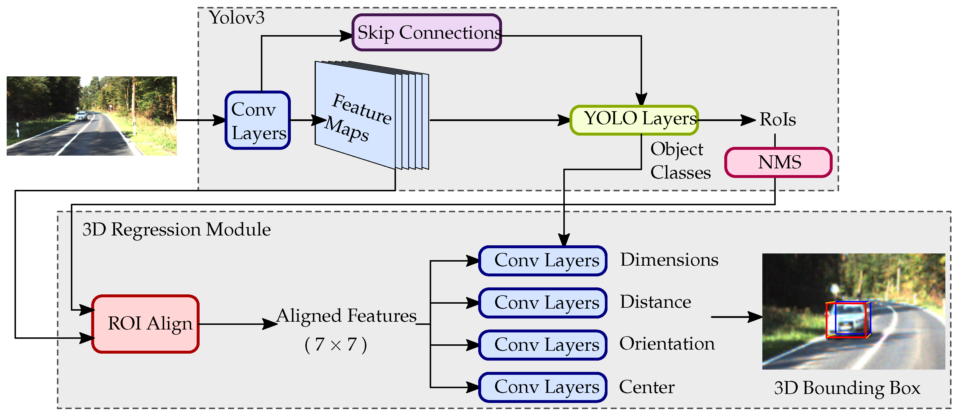
- A new method for a real-time multi-class 3D object detection network that is trainable end-to-end. We leverage the popular real-time object detector You Only Look Once (YOLO) v3 for regions of interest (RoIs) prediction used in our network. Our methods allow the following predictions:
- Object 2D detection;
- Object distance from the camera;
- Object 3D centers projected on the image plane;
- Object 3D dimension and orientation.
With these predictions, our method is able to draw 3D bounding boxes for the objects. - A new photo-realistic virtual multi-modal dataset for 3D detection in the road and railway environment using the video game Grand Theft Auto (GTA) V. The GTAV dataset includes images taken from the point of view of both cars and trains.
2. Related Work
2.1. 3D Object Detection from a Depth Sensor
2.2. 3D Object Detection from Monocular Images
3. Our Realtime 3D Multi-Object Detection and Localization Network
3.1. 3D Bounding Estimation
3.2. Parameters to Regress
3.3. Losses
4. Experimental Results
4.1. Training Details
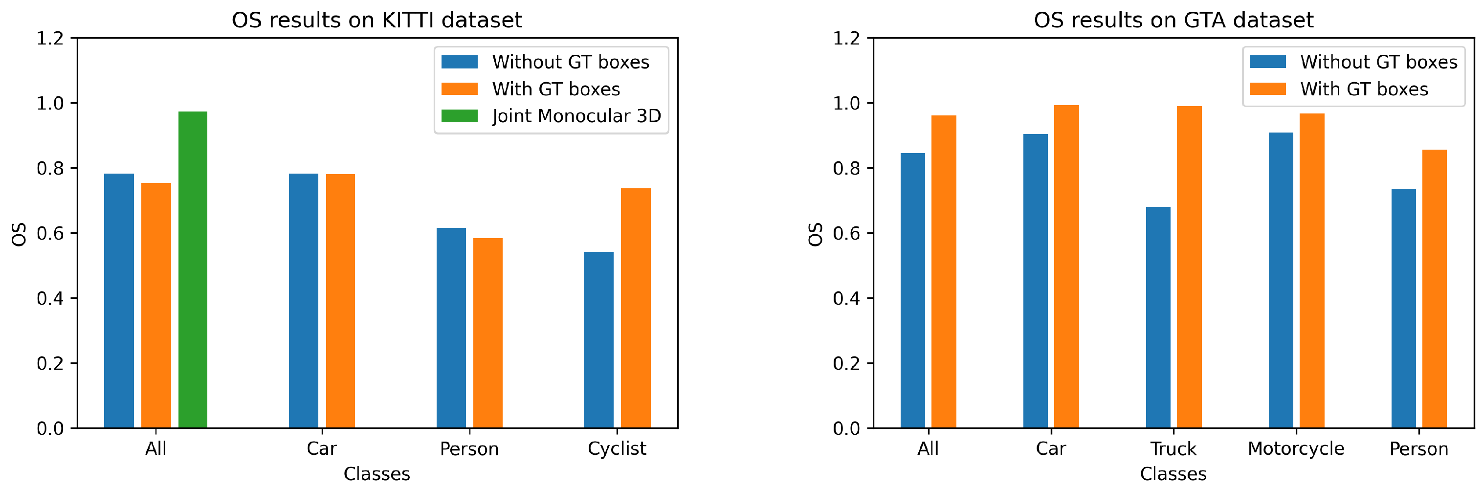
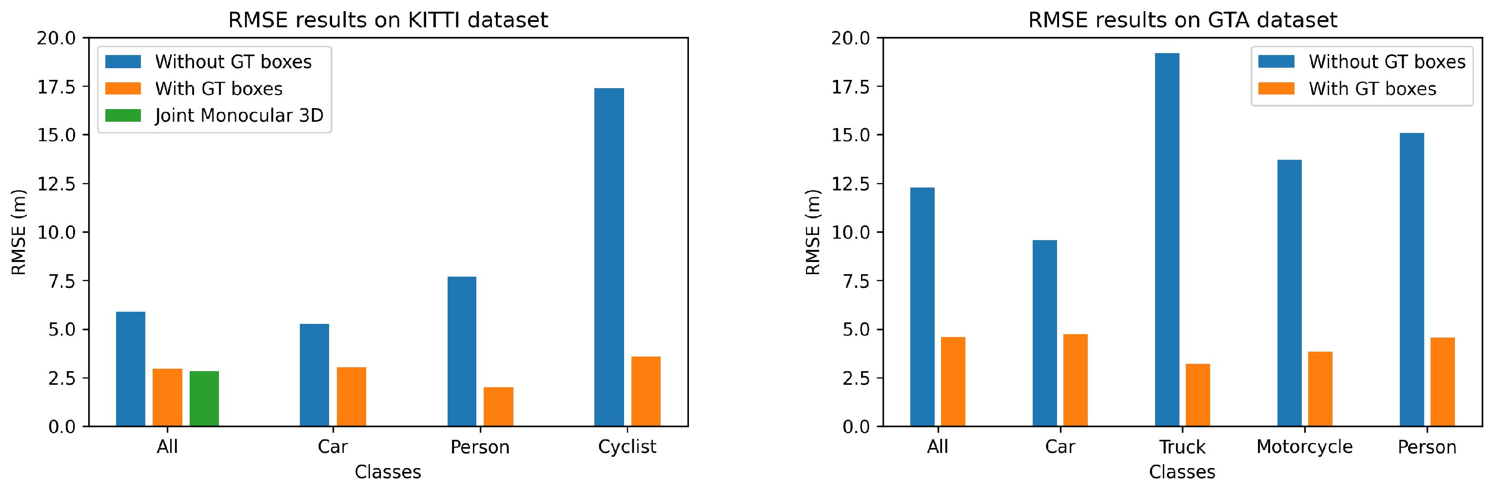
4.2. Evaluation
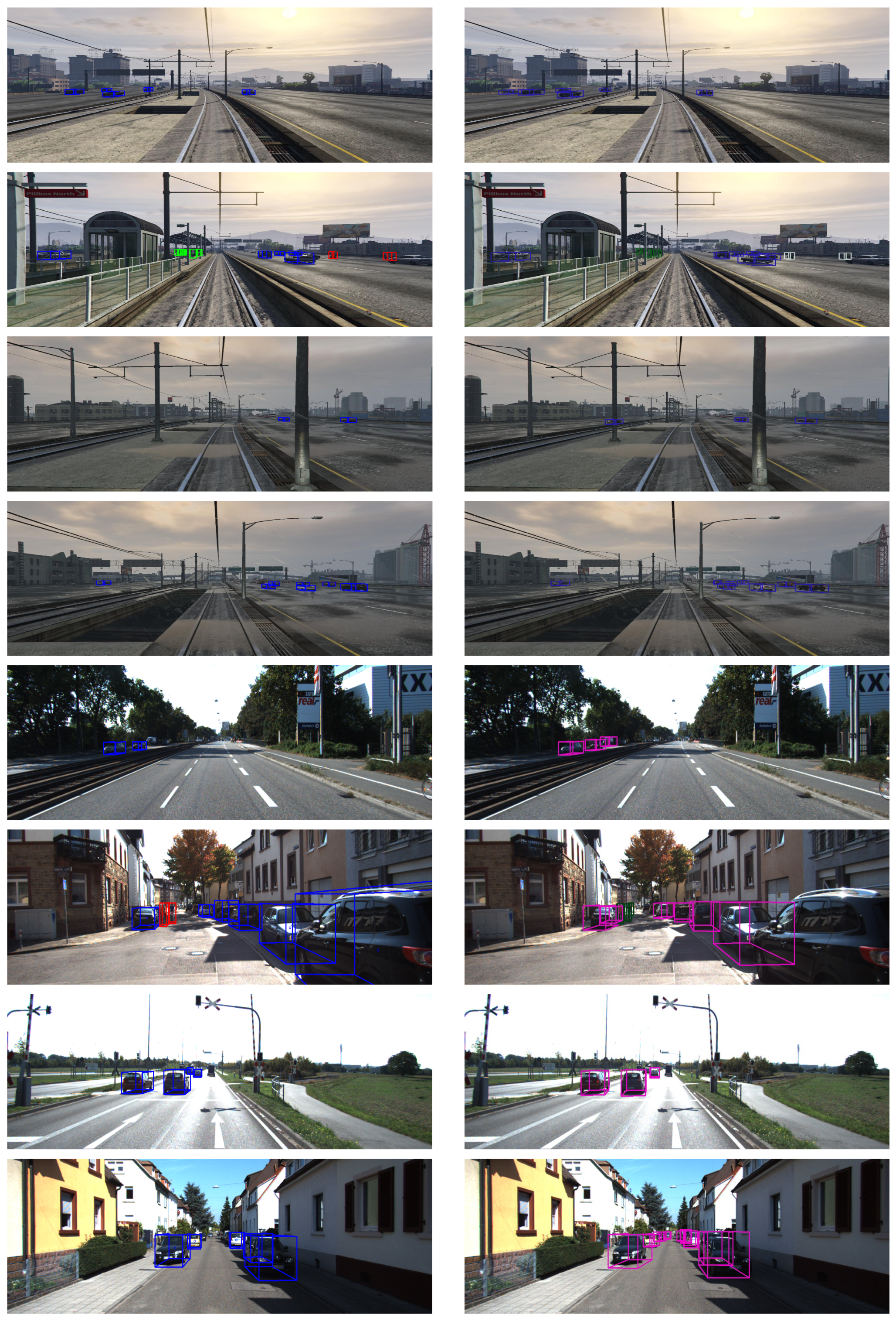
4.3. Results
5. Conclusions
Author Contributions
Funding
Institutional Review Board Statement
Informed Consent Statement
Data Availability Statement
Acknowledgments
Conflicts of Interest
Abbreviations
| ADAS | Advanced driver-assistance system |
| GTA | Grand Theft Auto |
| ToF | Time of flight |
| CNN | Convolutional neural networks |
| MLP | Multi-layer perceptron |
| PointRGCN | Pipeline based on graph convolutional networks |
| RoIs | Regions of interest |
| RPN | Region proposal network |
| NMS | Non-maximum suppression |
| GCN | Graph convolutional networks |
| ARE | Absolute relative error |
| RMSE | Root-mean-square error |
| BMP | Bad matching pixels |
| DS | Dimension score |
| CS | Center score |
| OS | Orientation score |
| YOLO | You only look once |
| LiDAR | Light detection and ranging |
| GT | Ground truth |
References
- Zhao, M.; Mammeri, A.; Boukerche, A. Distance measurement system for smart vehicles. In Proceedings of the 2015 7th International Conference on New Technologies, Mobility and Security (NTMS), Paris, France, 27–29 July 2015; pp. 1–5. [Google Scholar]
- Palacín, J.; Pallejà, T.; Tresanchez, M.; Sanz, R.; Llorens, J.; Ribes-Dasi, M.; Masip, J.; Arno, J.; Escola, A.; Rosell, J.R. Real-time tree-foliage surface estimation using a ground laser scanner. IEEE Trans. Instrum. Meas. 2007, 56, 1377–1383. [Google Scholar] [CrossRef] [Green Version]
- Kang, B.; Kim, S.J.; Lee, S.; Lee, K.; Kim, J.D.; Kim, C.Y. Harmonic distortion free distance estimation in ToF camera. In Three-Dimensional Imaging, Interaction, and Measurement; International Society for Optics and Photonics: Bellingham, WA, USA, 2011; Volume 7864, p. 786403. [Google Scholar]
- Qi, C.R.; Su, H.; Mo, K.; Guibas, L.J. PointNet: Deep Learning on Point Sets for 3D Classification and Segmentation. arXiv 2017, arXiv:cs.CV/1612.00593. [Google Scholar]
- Zarzar, J.; Giancola, S.; Ghanem, B. PointRGCN: Graph Convolution Networks for 3D Vehicles Detection Refinement. arXiv 2019, arXiv:cs.CV/1911.12236. [Google Scholar]
- Chang, A.X.; Funkhouser, T.; Guibas, L.; Hanrahan, P.; Huang, Q.; Li, Z.; Savarese, S.; Savva, M.; Song, S.; Su, H.; et al. ShapeNet: An Information-Rich 3D Model Repository. arXiv 2015, arXiv:cs.GR/1512.03012. [Google Scholar]
- Geiger, A.; Lenz, P.; Stiller, C.; Urtasun, R. Vision meets robotics: The KITTI dataset. Int. J. Robot. Res. 2013, 32, 1231–1237. [Google Scholar] [CrossRef] [Green Version]
- Ku, J.; Mozifian, M.; Lee, J.; Harakeh, A.; Waslander, S. Joint 3D Proposal Generation and Object Detection from View Aggregation. arXiv 2018, arXiv:cs.CV/1712.02294. [Google Scholar]
- Chen, X.; Kundu, K.; Zhang, Z.; Ma, H.; Fidler, S.; Urtasun, R. Monocular 3D object detection for autonomous driving. In Proceedings of the 2016 IEEE Conference on Computer Vision and Pattern Recognition (CVPR), Las Vegas, NV, USA, 27–30 June 2016; pp. 2147–2156. [Google Scholar] [CrossRef]
- Mousavian, A.; Anguelov, D.; Flynn, J.; Kosecka, J. 3D Bounding Box Estimation Using Deep Learning and Geometry. arXiv 2017, arXiv:cs.CV/1612.00496. [Google Scholar]
- Hu, H.N.; Cai, Q.Z.; Wang, D.; Lin, J.; Sun, M.; Krähenbühl, P.; Darrell, T.; Yu, F. Joint Monocular 3D Vehicle Detection and Tracking. arXiv 2019, arXiv:cs.CV/1811.10742. [Google Scholar]
- Chabot, F.; Chaouch, M.; Rabarisoa, J.; Teulière, C.; Chateau, T. Deep MANTA: A Coarse-to-fine Many-Task Network for joint 2D and 3D vehicle analysis from monocular image. arXiv 2017, arXiv:cs.CV/1703.07570. [Google Scholar]
- Redmon, J.; Farhadi, A. Yolov3: An incremental improvement. arXiv 2018, arXiv:1804.02767. [Google Scholar]
- Wu, Y.; Kirillov, A.; Massa, F.; Lo, W.Y.; Girshick, R. Detectron2. Available online: https://github.com/facebookresearch/detectron2 (accessed on 29 September 2019).
- Richter, S.R.; Vineet, V.; Roth, S.; Koltun, V. Playing for data: Ground truth from computer games. In European Conference on Computer Vision (ECCV); Leibe, B., Matas, J., Sebe, N., Welling, M., Eds.; Springer International Publishing: Berlin/Heidelberg, Germany, 2016; Volume 9906, pp. 102–118. [Google Scholar]
- Smith, L.N.; Topin, N. Super-Convergence: Very Fast Training of Neural Networks Using Large Learning Rates. arXiv 2018, arXiv:cs.LG/1708.07120. [Google Scholar]
- Zendel, O.; Murschitz, M.; Zeilinger, M.; Steininger, D.; Abbasi, S.; Beleznai, C. RailSem19: A dataset for semantic rail scene understanding. In Proceedings of the IEEE Conference on Computer Vision and Pattern Recognition Workshops, Long Beach, CA, USA, 16–20 June 2019; pp. 1221–1229. [Google Scholar]


| Dataset | Method | 2D Detection | Distance | Dimensions DS | Center CS | Orientation OS | VRAM Usage | Inference Time | |||||||||
|---|---|---|---|---|---|---|---|---|---|---|---|---|---|---|---|---|---|
| AP | R | mAP | F1 | Abs Rel | SRE | RMSE (m) | log RMSE | ||||||||||
| KITTI | Ours (w GT RoIs) | - | - | - | - | 0.096 | 0.307 | 2.96 | 0.175 | 0.941 | 0.980 | 0.988 | 0.847 | 0.983 | 0.753 | 3.22 GB | 10 ms |
| Ours (w/o GT RoIs) | 0.469 | 0.589 | 0.5 | 0.517 | 0.199 | 2.32 | 5.89 | 0.310 | 0.823 | 0.934 | 0.960 | 0.853 | 0.951 | 0.765 | 3.22 GB | 10 ms | |
| Joint Monocular 3D [11] | - | - | - | - | 0.074 | 0.449 | 2.847 | 0.126 | 0.954 | 0.980 | 0.987 | 0.962 | 0.918 | 0.974 | 5.64 GB | 97 ms | |
| GTA | Ours (w GT RoIs) | - | - | - | - | 0.069 | 0.420 | 4.60 | 0.100 | 0.965 | 0.992 | 0.999 | 0.886 | 0.999 | 0.961 | 3.22 GB | 10 ms |
| Ours (w/o GT RoIs) | 0.533 | 0.763 | 0.632 | 0.61 | 0.207 | 4.92 | 12.3 | 0.319 | 0.781 | 0.897 | 0.942 | 0.853 | 0.846 | 0.845 | 3.22 GB | ||
| Dataset | Classes | Method | 2D Detection | Distance | Dimensions | Center | Orientation | |||||||||
|---|---|---|---|---|---|---|---|---|---|---|---|---|---|---|---|---|
| AP | R | mAP | F1 | Abs Rel | SRE | RMSE (m) | log RMSE | DS | CS | OS | ||||||
| KITTI | Car | Ours (w GT RoIs) | - | - | - | - | 0.0957 | 0.312 | 3.05 | 0.18 | 0.941 | 0.980 | 0.988 | 0.872 | 0.981 | 0.781 |
| Ours (w/o GT RoIs) | 0.558 | 0.879 | 0.783 | 0.682 | 0.163 | 1.29 | 5.28 | 0.271 | 0.839 | 0.948 | 0.971 | 0.867 | 0.962 | 0.783 | ||
| Person | Ours (w GT RoIs) | - | - | - | - | 0.0979 | 0.254 | 2.01 | 0.154 | 0.935 | 0.983 | 0.992 | 0.705 | 0.993 | 0.584 | |
| Ours (w/o GT RoIs) | 0.508 | 0.518 | 0.464 | 0.513 | 0.424 | 7.92 | 7.70 | 0.485 | 0.729 | 0.844 | 0.892 | 0.719 | 0.885 | 0.616 | ||
| Cyclist | Ours (w GT RoIs) | - | - | - | - | 0.0979 | 0.359 | 3.57 | 0.150 | 0.940 | 0.979 | 0.988 | 0.809 | 0.997 | 0.738 | |
| Ours (w/o GT RoIs) | 0.342 | 0.371 | 0.253 | 0.356 | 1.04 | 30.9 | 17.4 | 0.797 | 0.415 | 0.622 | 0.719 | 0.812 | 0.678 | 0.542 | ||
| GTA | Car | Ours (w GT RoIs) | - | - | - | - | 0.0552 | 0.385 | 4.74 | 0.0761 | 0.990 | 0.999 | 0.999 | 0.860 | 0.999 | 0.993 |
| Ours (w/o GT RoIs) | 0.477 | 0.915 | 0.778 | 0.627 | 0.129 | 2.28 | 9.59 | 0.217 | 0.873 | 0.938 | 0.965 | 0.812 | 0.894 | 0.905 | ||
| Truck | Ours (w GT RoIs) | - | - | - | - | 0.0454 | 0.178 | 3.22 | 0.0576 | 0.994 | 1.00 | 1.00 | 0.871 | 0.999 | 0.989 | |
| Ours (w/o GT RoIs) | 0.312 | 0.880 | 0.617 | 0.461 | 0.259 | 6.99 | 19.2 | 0.455 | 0.642 | 0.78 | 0.868 | 0.736 | 0.622 | 0.681 | ||
| Motorcycle | Ours (w GT RoIs) | - | - | - | - | 0.0623 | 0.266 | 3.84 | 0.0753 | 1.00 | 1.00 | 1.00 | 0.918 | 1.00 | 0.967 | |
| Ours (w/o GT RoIs) | 0.614 | 0.764 | 0.725 | 0.681 | 0.186 | 3.58 | 13.7 | 0.281 | 0.691 | 0.878 | 0.967 | 0.901 | 0.689 | 0.909 | ||
| Person | Ours (w GT RoIs) | - | - | - | - | 0.116 | 0.612 | 4.56 | 0.159 | 0.877 | 0.966 | 1.00 | 0.963 | 0.997 | 0.856 | |
| Ours (w/o GT RoIs) | 0.263 | 0.659 | 0.488 | 0.375 | 0.372 | 10.5 | 15.1 | 0.453 | 0.620 | 0.834 | 0.903 | 0.961 | 0.812 | 0.735 | ||
Publisher’s Note: MDPI stays neutral with regard to jurisdictional claims in published maps and institutional affiliations. |
© 2021 by the authors. Licensee MDPI, Basel, Switzerland. This article is an open access article distributed under the terms and conditions of the Creative Commons Attribution (CC BY) license (https://creativecommons.org/licenses/by/4.0/).
Share and Cite
Mauri, A.; Khemmar, R.; Decoux, B.; Haddad, M.; Boutteau, R. Real-Time 3D Multi-Object Detection and Localization Based on Deep Learning for Road and Railway Smart Mobility. J. Imaging 2021, 7, 145. https://0-doi-org.brum.beds.ac.uk/10.3390/jimaging7080145
Mauri A, Khemmar R, Decoux B, Haddad M, Boutteau R. Real-Time 3D Multi-Object Detection and Localization Based on Deep Learning for Road and Railway Smart Mobility. Journal of Imaging. 2021; 7(8):145. https://0-doi-org.brum.beds.ac.uk/10.3390/jimaging7080145
Chicago/Turabian StyleMauri, Antoine, Redouane Khemmar, Benoit Decoux, Madjid Haddad, and Rémi Boutteau. 2021. "Real-Time 3D Multi-Object Detection and Localization Based on Deep Learning for Road and Railway Smart Mobility" Journal of Imaging 7, no. 8: 145. https://0-doi-org.brum.beds.ac.uk/10.3390/jimaging7080145