Mathematical Modeling of Heat Transfer in an Element of Combustible Plant Material When Exposed to Radiation from a Forest Fire


School of Energy and Power Engineering, Tomsk Polytechnic University, Tomsk 634050, Russia
*
Author to whom correspondence should be addressed.
Safety 2019, 5(3), 56; https://0-doi-org.brum.beds.ac.uk/10.3390/safety5030056
Submission received: 6 June 2019
/
Revised: 18 July 2019
/
Accepted: 11 August 2019
/
Published: 15 August 2019
(This article belongs to the Special Issue Fire Safety 2019)
Abstract
:The last few decades have been characterized by an increase in the frequency and burned area of forest fires in many countries of the world. Needles, foliage, branches, and herbaceous plants are involved in burning during forest fires. Most forest fires are surface ones. The purpose of this study was to develop a mathematical model of heat transfer in an element of combustible plant material, namely, in the stem of a herbaceous plant, when exposed to radiation from a surface forest fire. Mathematically, the process of heat transfer in an element of combustible plant material was described by a system of non-stationary partial differential equations with corresponding initial and boundary conditions. The finite difference method was used to solve this system of equations in combination with a locally one-dimensional method for solving multidimensional tasks of mathematical physics. Temperature distributions were obtained as a result of modeling in a structurally inhomogeneous stem of a herbaceous plant for various scenarios of the impact of a forest fire. The results can be used to develop new systems for forest fire forecasting and their environmental impact prediction.
1. Introduction
During surface forest fires, various forest fuels and combustible plant materials are involved in combustion processes [1], including herbaceous plants [2]. Such plants have a different structure. Herbaceous plants belonging to grass species often grow in forested areas. Various morphological parts (elements) can be marked out in the structure of such plants: stem, spikelet, leaf blade. This paper discusses the stem of a herbaceous plant [3]. A surface forest fire was chosen to act on the stem of the herbaceous plant [4], since most forest fires are surface forest fires. The overwhelming majority of crown forest fires develop from surface fires [5]. The processes of heat transfer in the combustible plant material play an important role in the ignition of these fires, as well as the propagation of the forest fire line over a layer of combustible plant material.
It should be noted that it is important to understand the process of heat transfer in vegetable fuel material because it affects the mass transfer in vegetable fuel material, and also causes many processes associated with the occurrence of a forest fire or grassland fire. The fires themselves play different roles in the formation and functioning of grasslands and forest stands. Fires can affect the near-surface soil layer, causing changes in the functioning of microbial communities and the chemical composition of the soil and causing water soil erosion [6,7,8,9]. On the other hand, during the combustion of combustible plant materials, large amounts of various gaseous substances are released into the atmosphere, including those that lead to the greenhouse effect and climate change on the planet [10,11]. Measurements using ground-based tools, aircraft, and balloons have shown that, as a result of natural fires, carbon dioxide, carbon monoxide, and methane emissions, as well as small particles of black carbon, occur in large volumes. These measurements showed that emission factors for forest and grassland fires are different by a factor of two. An understanding of the processes of heat transfer in the structure of combustible plant material is obviously necessary. In addition, mathematical models of heat transfer in vegetative fuel can be used in conjunction with information obtained from satellite systems [12]. The abovementioned aspects of forest fire danger determines the following research objective.
The purpose of the study was to develop a mathematical model of heat transfer in an element of combustible plant material, namely, in the stem of a herbaceous plant, when exposed to radiation from a surface forest fire. This mathematical model aimed to construct program instruments in GIS-systems to predict forest fire danger and fuel management.
2. Background
A forest fire is a spontaneous, uncontrollable spread of fire over forest areas [13]. The causes of fires in the forest can be divided into natural and man-made [14]. The most common natural causes of large forest fires on Earth are thunderstorms [15]. In young forests, in which there is a lot of greenery, the probability of fire from lightning is significantly lower than in aged forests, where there are many dry and diseased trees [16]. The ecological role of forest fires was formerly the natural renewal of forests [17]. However, in recent decades, forest fires have gone from being a natural regulatory factor to a catastrophic phenomenon [18]. Sometimes fires are caused artificially. Such fires are called prescribed [19]. The goal of prescribed fires is the destruction of fire-hazardous combustible materials, the removal of logging waste, the preparation of planting sites for seedlings, the fight against insects and forest diseases, etc.
Depending on where the fire spreads, fires are divided into surface, crown, and soil fires [4]. Surface fire is a significant disturbance factor in forests. Forest litter, lichens, mosses, grasses, and fallen branches burn during surface fires. The speed of fire movement in the wind is 0.25–5 km/h. The height of the flames is up to 2.5 m. The burning temperature is about 700 °C (sometimes higher).
A fluent surface fire burns the upper part of the ground cover, undergrowth, and underbrush. Such a fire spreads with great speed, bypassing places with high humidity, so parts of the area remain unaffected by fire. Fluent fires mainly occur in the spring, when only the topmost layer of small combustible materials dries out.
Steady surface fires spread slowly, with the living and dead ground cover completely burning out, the roots and bark of the trees burning very strongly, and the undergrowth and undergrowth burning down completely. Steady surface fires occur predominantly from mid-summer onwards.
A forest area is a significant integral forest territory, having natural borders (rivers, lakes, hills, separate parts of mountainous terrain) or bordering on a large distance with other lands (fields, meadows) or populated areas. A forest may have conditional boundaries, depending on the purpose of the forest, its proximity to transport routes, and points of removal and consumption. Its area may range from several hundred to several thousand hectares [20,21].
Depending on the biological characteristics of the most important plants, their age, and certain physiographic conditions in the forest, several tiers of plants develop. Longlines are fairly well-defined horizons of concentration of the active organs of plants. Longlines can be formed by one or two or more species [4]. Grass or grass–shrub tier can be marked out in the forest stand.
The processes of physicochemical reaction are due to heat transfer in the combustible plant material. One of the stages of ignition of combustible materials is their thermal decomposition (pyrolysis). From the point of view of the development of new mathematical models of forest fuel ignition, a simplified model of the pyrolysis of a polymeric material with regard to the transport of volatile compounds is of interest [22]. It should be noted that the problem of gasification of solids has been widely described in the literature, for example, in the review by Di Blasi [23]. The simplest approach to this problem implies that a solid decomposes with the release of volatile compounds directly at a critical temperature [22]. Accordingly, the critical temperature is a task parameter. This approach (often called the ablative model) is mathematically analogous to the problem of Stefan [24], and its variation with respect to the thawing process was described in the classic article by Landau [25] and later implemented in a number of papers, for example by Billings et al. and Whiting et al. [26,27]. The second approach includes a kinetic mechanism for the decomposition process, which is usually established as a result of thermogravimetric analysis. A fairly representative description of this approach can be found in References [28,29]. In Reference [22], the effect of a simple volatile transport mechanism in a transit model of polymer pyrolysis, which also takes into account the change in sample volume, was considered. The equations used for the variation with time of the mass and volume of the sample subjected to pyrolysis are given, as well as the energy equation (heat conduction equation). The model was closed by the expression for the speed of movement of volatile pyrolysis products [29]. The effects of external heat flux, and convective and radiative heat exchange with the environment were taken into account in the boundary conditions.
There have been many works on the experimental and theoretical study of the pyrolysis of cellulosic materials [30,31,32,33]. These studies have mainly focused on the effects of heat flux, size, moisture content, chemical composition of the sample and structural heterogeneity of the temperature distribution, decomposition of solids, and the rate of evolution of volatile compounds. Reference [34] also investigated the processes of thermal decomposition of moist wood under the influence of external heat flux. An experimental setup was created on the basis of a calorimeter that supported the heating mode in the range of heat fluxes from 0 to 80 kW/m2. Birch samples with different moisture contents (about 5%, 15%, and 26%) were studied. Several thermocouples were built into the samples at various locations to record the temperature along the center line. Samples were also measured. The temperature and mass of the sample were recorded in 1 s increments. It was found that the sample began to lose moisture if the temperature exceeded 100 °C. The loss of mass was slowed below 240 °C and the gases did not ignite. In the range of 240–320 °C, the pyrolysis process was endothermic and the gases mainly consisted of carbon dioxide and water vapor. Starting from 320 °C, pyrolysis took place very quickly, with the release of a large amount of combustible gases. A kinetic scheme for wet wood pyrolysis was established, which included charring, the formation of gaseous pyrolysis products, and water vapor. A mathematical model of pyrolysis was developed for comparative analysis with experimental data [34].
The bulk density and fuel load have an impact on the occurrence and spread of fire in grasslands [35]. These parameters are used in many forest fire management systems, such as forecasting and assessing forest fire danger [36,37], fire behavior assessment [38,39], and in forest fuel management systems [40,41,42]. As a rule, the fuel load is directly proportional to the energy that is released as a result of burning. Accordingly, the greater the fuel load, the more energy is released in the front of the fire [35]. It should be noted that the grass can be in a living, dried, or dead state, depending on the biophysical characteristics. Many herbaceous plants are perennial. For the purposes of monitoring, forecasting, and evaluating forest fire danger, it is important to understand how much vegetation is in a dead state. This is especially important when predicting a fire hazard in grasslands [43]. The authors of Reference [43] have developed a method for estimating the amount of dead grass based on spectral reflection. Soil and dead grass samples were collected and laboratory measurements were subsequently made. Spectral reflection was measured for samples with different densities and for different wavelengths (350–2500 nm). As a result, a new spectral index was developed, which can be used with satellite images of the Moderate-resolution Imaging Spectroradiometers (MODIS) instrument from the Terra/Aqua satellite system. On the other hand, spectral indices can be used to assess burn severity in grasslands [44]. These estimates can be made using Landsat imagery. Again, mathematical modeling of heat transfer can be used to jointly evaluate burn severity from ground data. As practice shows [45], the joint use of ground-based and satellite observations is the most promising method for obtaining spatial information about grass-covered areas.
Another important parameter determining the ability of combustible plant material to ignite is its moisture content [46]. The moisture content of combustible plant material plays a key role in ignition of the combustible material and the fire spreading through a layer of combustible material. Depending on moisture content, vegetation can both serve as a conductor of burning and slow down the spread of fire [47]. In addition, the moisture content of the combustible plant material influences the effective thermophysical characteristics of the material, causing differences in the processes of pre-heating the combustible plant material [48].
It should also be noted that, to date, various approaches have been used to predict the spread of fire over grassland. For example, empirical [49], physically based [50], and statistical [51] methods are known. It is important to understand the range of values in which the density of the radiant heat flux in grassland fires falls. In Reference [52], it was found that in the front of a grassland fire, the radiant heat flux density was about 26–45 kW/m2. This was in close proximity to the burning zone. It should be borne in mind that the density of the incident radiant heat flux on the element of combustible material will depend on the distance from the fire front to the herbaceous plant.
3. Study Area and Object
The study was conducted in the Gilbirinskiy forestland (Ivolginskiy district of the Republic of Buryatia, Figure 1) in a protected natural area. The study area is located between latitudes 51°35′50″ N and 51°46′40″ N and longitudes 106°42′ E and 107°02′ E [53]. This area is 55 km southeast of Lake Baikal, and belongs to the northern tip of the Selenga middle mountain (Figure 1). The area of the forestland is about 270 km2 [54]. The forestland was divided into 126 forest areas. The forest quarter is a part of the forestland and it has permanent boundaries. The forest quarter is the main accounting unit of the forest fund in the Russian Federation.
The study region, like the whole of Buryatia, has a sharply continental climate, with cold winters and hot summers. The average temperature in summer is about +18.5 °C, in winter is about −22 °C, and the average annual temperature is about −1.6 °C. The average annual rainfall is 244 mm. A significant feature of the climate is the long duration of sunshine for 1900–2200 hours per year [55].
About 90% of the territory is occupied by natural plantations. There are types of glades, slopes, pebbles, forest cultures, arable land, pastures, etc. The main forest-forming species are larch, pine, cedar, birch, and aspen [56].
The main functions of forests located in water protection zones are to prevent pollution, clogging, siltation of water bodies, and depletion of their waters, as well as to preserve the habitat of aquatic biological resources and other objects of the animal and plant world.
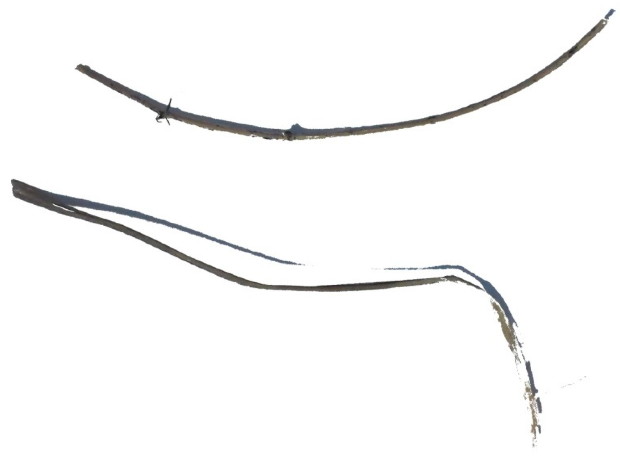
The use of forests for agriculture can include use for haying, grazing of farm animals, honey bearing plants and grasses, growing crops, etc. Figure 2 shows images of the typical elements of combustible plant material: the stem and leaf blades. A joint in the center can be seen on the stem.
As a prototype for building a geometric model, a stem of grass was used. The stem was partially brown and dried. The material was collected in the Gilbirinskiy forestland of the Republic of Buryatia in the spring of 2018.
4. Physical Model
The following physical model of heat transfer in combustible plant material was considered. A herbaceous plant grows in some forested area. A single element is considered, namely, the stem. Near the plant, there is an active surface forest fire. A radiant heat flux acts from the forest fire line on the element of the combustible plant material. Inert heating of the element of combustible plant material occurs. When the temperature rises, thermal decomposition of the dry organic matter of the combustible plant material occurs.
The following assumptions were applied to the physical model:
- (1)
- The spring season of the fire season is considered and the grass is dried.
- (2)
- The catastrophic scenario of forest fire danger is considered when moisture in the forest fuel material is absent.
- (3)
- The evaporation of moisture is neglected.
- (4)
- The thermophysical characteristics do not depend on temperature.
- (5)
- The pyrolysis of dry organic matter is considered as a one-step process with known thermokinetic constants.
- (6)
- The two-dimensional formulation of the problem is considered.
- (7)
- The process of heat transfer in the element of combustible plant material occurs due to thermal conductivity.
- (8)
- The main damaging factor of a forest fire is radiant heat flux, and other types of heat transfer are neglected.
- (9)
- The layered and structurally inhomogeneous composition of the combustible plant material is considered.
5. Mathematical Models
5.1. Simplified Mathematical Model of Heat Transfer in the Stem
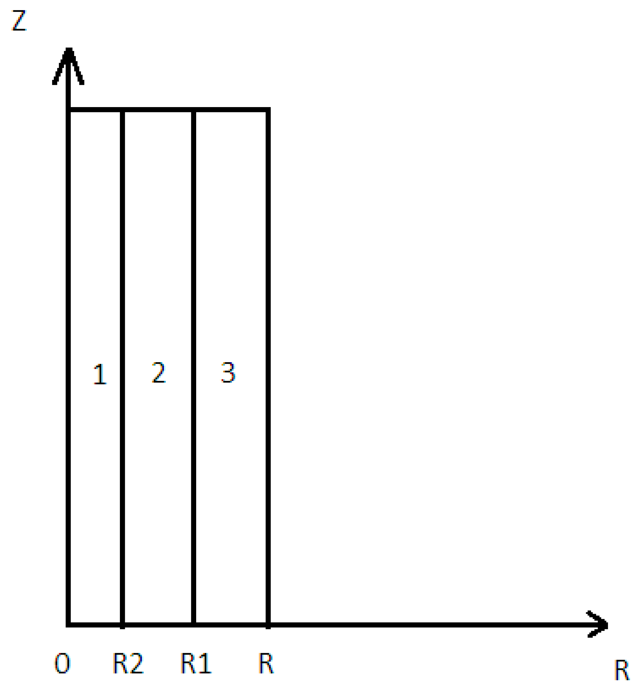
Figure 3 shows the geometry of the solution area, where 1 is the cavity, 2 is the pulp, and 3 is the protective skin.
Mathematically, heat transfer in the layered structure of the stem is described by a non-stationary heat conduction equation with the corresponding initial and boundary conditions:
The initial conditions:
The boundary conditions:
where Ti, ρi, ci, λi—temperature, density, heat capacity, and thermal conductivity of the stem layers (1—cavity, 2—pulp, 3—protective skin); r, z—spatial coordinates; t is the time coordinate; and qff is the radiant heat flux from the forest fire line. The finite difference method was used to solve the formulated system of equations. Difference analogues of differential equations were solved by the marched method. Two-dimensional partial differential equations were solved by the locally one-dimensional method [32,33].
5.2. Mathematical Model of Heat Transfer with the Joint
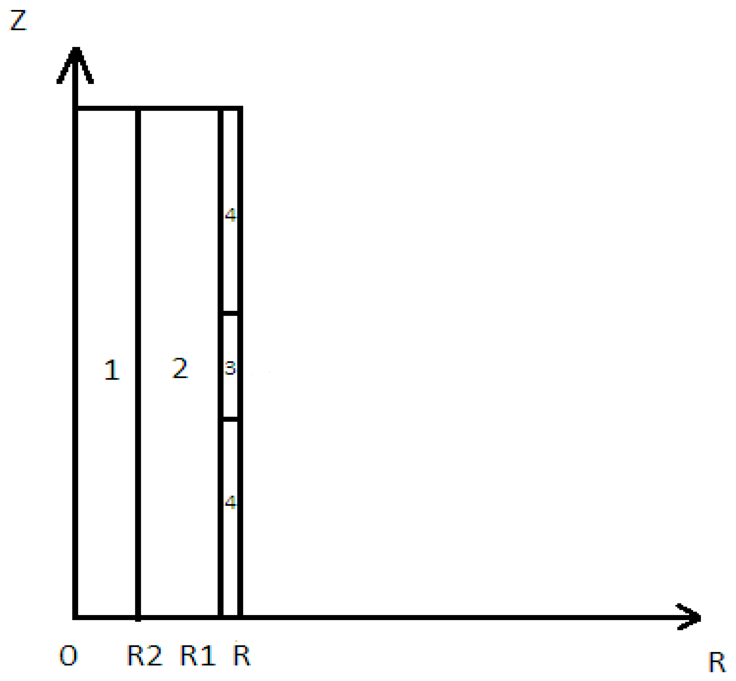
The geometry of the solution area is shown in Figure 4.
Mathematically, the process of heat transfer in an element of combustible plant material is described by a system of non-stationary nonlinear differential equations in partial derivatives, with corresponding initial and boundary conditions. Below is a mathematical model of heat transfer in the element of combustible plant material when exposed to radiation from a forest fire:
The initial conditions:
The boundary conditions:
where Ti, ρi, ci, λi—temperature, density, heat capacity, and thermal conductivity of the stem layers (1—pulp, 2—protective skin, 3—growth on the site of stem articulation, 4—air); r, z—spatial coordinates; t is the time coordinate; and qff is the radiant heat flux from the forest fire line. The finite difference method was used to solve the formulated system of equations. Difference analogues of differential equations were solved by the marched method. Two-dimensional partial differential equations were solved by the locally one-dimensional method [58,59].
6. Results and Discussion
The main scenarios of the surface forest fire impact on the element of combustible plant material were developed to carry out computational experiments. Descriptions of the main scenarios are given in Table A1, Table A2, Table A3, Table A4, Table A5 and Table A6.
An analysis of the results presented in Figure A1, Figure A2, Figure A3, Figure A4, Figure A5, Figure A6, Figure A7, Figure A8, Figure A9, Figure A10, Figure A11, Figure A12, Figure A13 and Figure A14 showed that a low temperature field was formed in the central part of the stem near the soil. This was due to the lower temperature of the soil relative to the layer of vegetation and the ambient air temperature. In turn, the radiant heat flux from the forest fire line affected the side surface and it warmed up more intensely in comparison with the central part of the stem. Over time, the depth of heat penetration increased. It is also logical that at higher heat fluxes, a higher temperature was observed along the layers of the stem of the herbaceous plant. It should be noted that the hollow structure of the stem is characteristic of many herbaceous plants. Moisture is transported in the pulp, which is located between the cavity and the protective skin of the stem. In the simulation scenarios, a single soil temperature was used around the stem of a herbaceous plant. This allowed us to carry out a parametric study of the mathematical model by varying the structural characteristics of the stem and the parameters of the external influence of a forest fire. In the future, the effect of soil temperature during the day and season on the conditions of heat distribution in the stem under the influence of a forest fire should be assessed.
It should also be noted that in addition to the values used for the thermophysical characteristics of dry organic matter, other close quantitative values were used for other combustible plant materials. Computational experiments showed that there were no significant differences in heat transfer for various herbaceous plants in a dry state. It is important to understand that in the vegetative state, the moisture content of various herbaceous plants may differ significantly. This question requires a separate study in conjunction with the development of mathematical models of moisture transport in the stems of herbaceous plants, as well as the evaporation of free and bound moisture from an element of combustible plant material when exposed to radiation from a forest fire. It should also be noted that this article has discussed monolithic structure of the layers in the stem of a herbaceous plant. This assumption has been used for both the pulp and the protective skin of the joint. In a real situation, a developed porous structure is characteristic of these parts of the stem, which is especially important when considering the pulp of the stem. This has been shown by studies of the stem of a herbaceous plant under a microscope [60].
The size of a herbaceous plant (stem diameter) has an effect on the temperature distribution inside the stem structure. As the analysis of the results showed, the thicker the stem of a herbaceous plant was, the thicker the protective skin was on the outer part of the stem. The thermal conductivity of this layer was less compared with other layers of the stem. Radiant energy did not have time to penetrate into the stem and the surface layer of the stem was heated. This caused a temperature increase in this zone for a thicker stem of a herbaceous plant. It is safe to extrapolate the results obtained in this work to other species of herbaceous plants, both forest and agricultural. The exposure time affected the temperature distribution in the layered structure of the stem of a herbaceous plant. In a sense, exposure time and heat flux density characterize the location and speed of the forest fire line spread or an agricultural fire spread.
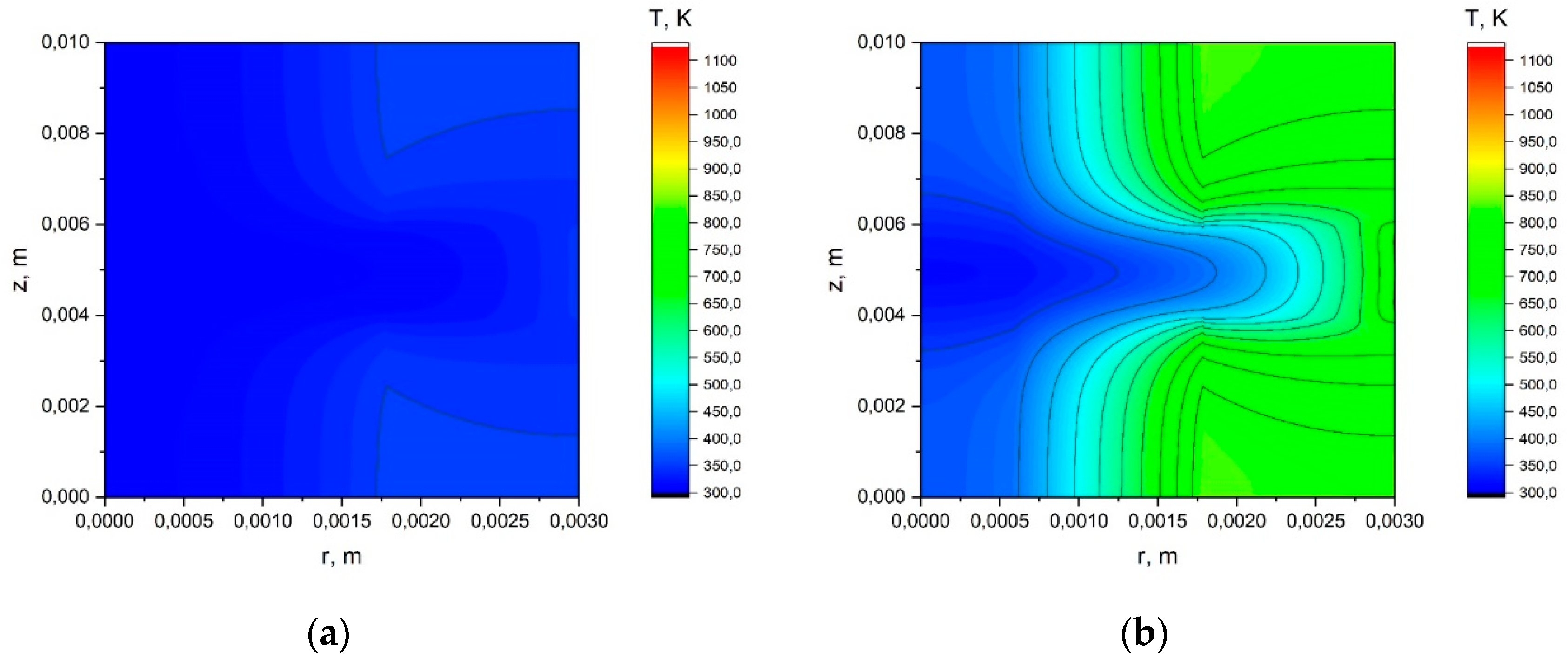
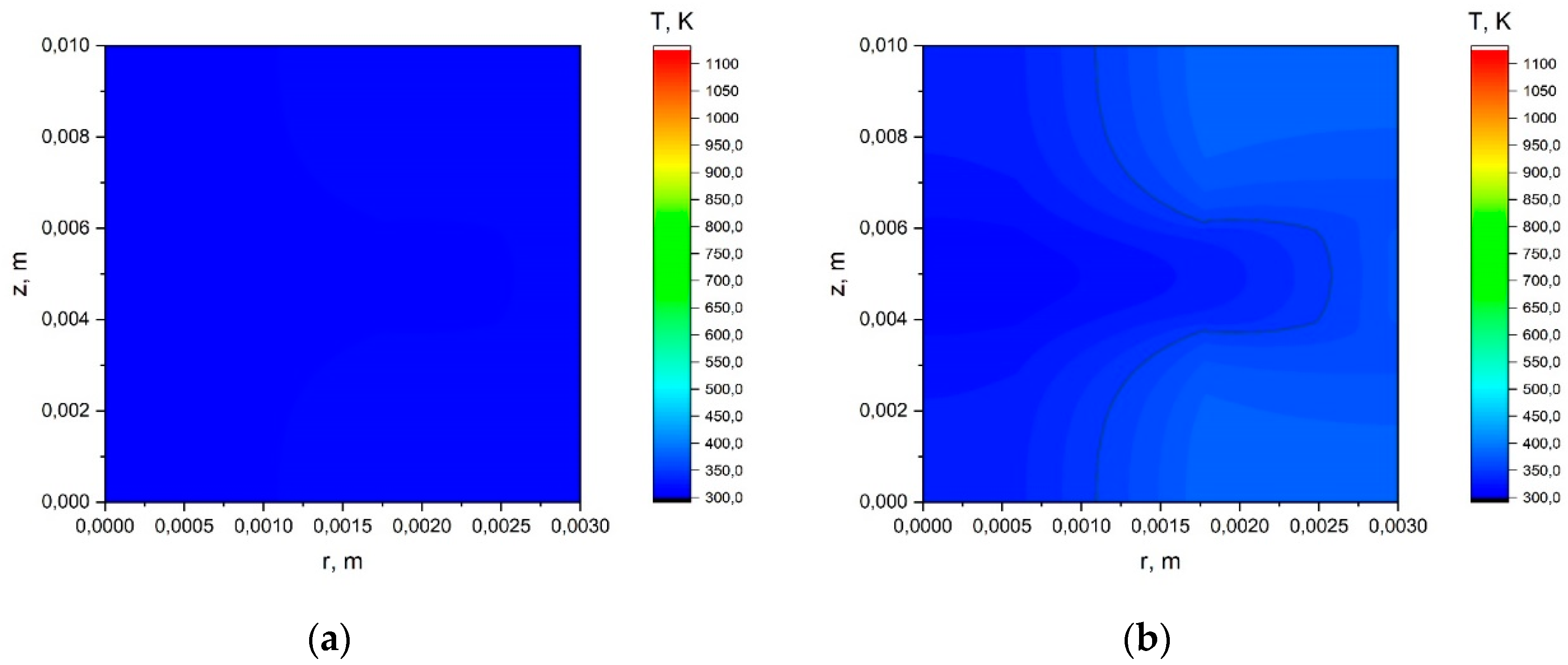
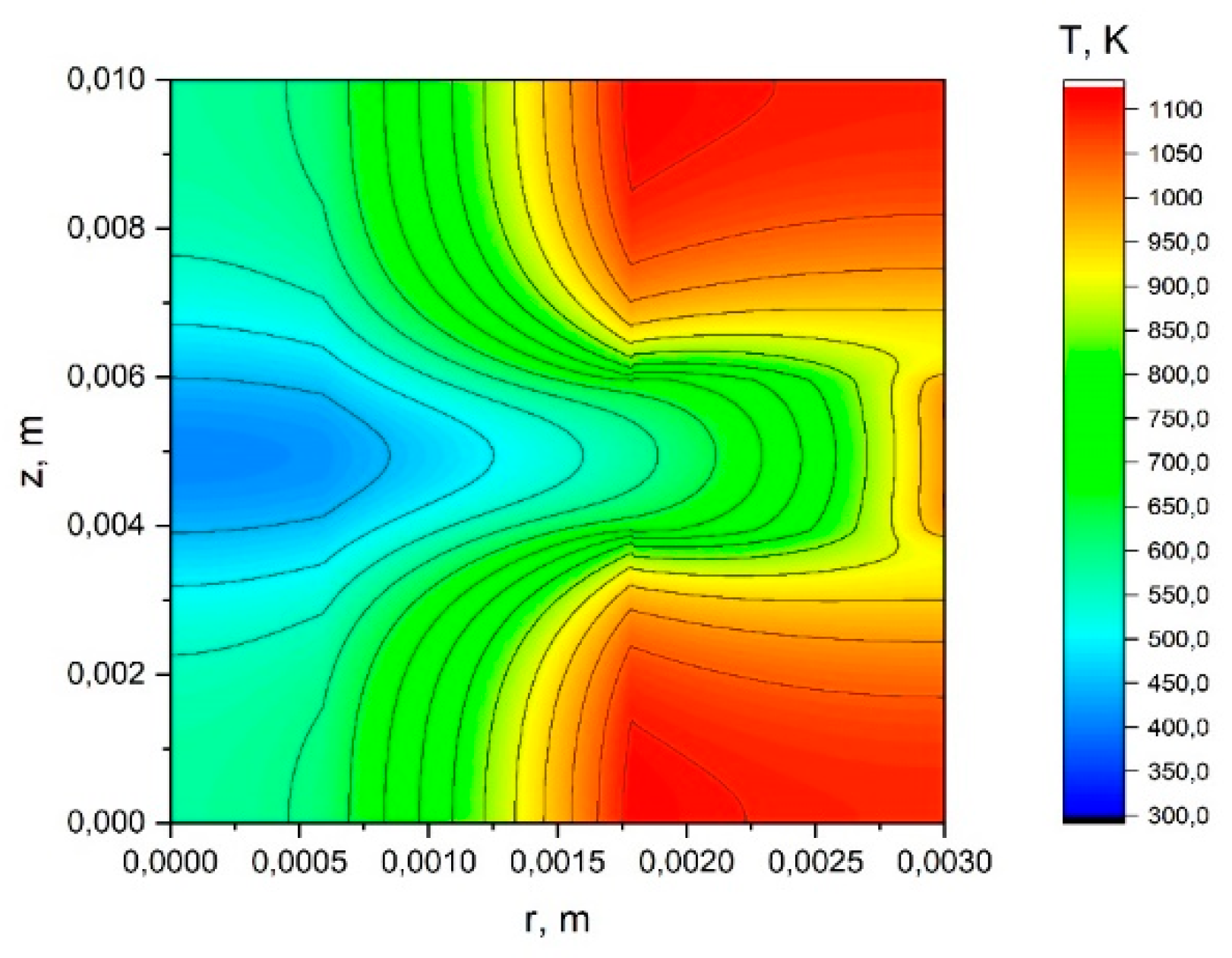
Figure A15, Figure A16, Figure A17, Figure A18, Figure A19, Figure A20, Figure A21, Figure A22, Figure A23, Figure A24, Figure A25, Figure A26, Figure A27 and Figure A28 show the results, the analysis of which allowed us to conclude that if a joint is located on the stem of a herbaceous plant, the temperature distributions become substantially non-uniform. This heterogeneity will be mainly due to structural heterogeneity. In the case of a fragment of the stem (solution region) being located above the soil layer, the heat transfer in the layered structure of the stem was not affected by the soil temperature at this height. However, in this variant there was a structural difference. There was no air cavity inside the stem, which somewhat changed the temperature distribution in this zone. This part was in this case occupied by the pulp. The main temperature changes occurred in the joint and the protective skin of the stem. The values of heat flux density and exposure time of radiation from a forest fire varied. The joint had a significant effect on the temperature distribution in the structurally inhomogeneous fragment of the stem of a herbaceous plant.
A forest fire is a multistep process in which the following stages can be marked out [4,61]: inert heating, evaporation of moisture, pyrolysis of dry organic matter, flammable combustion of gaseous combustible products of pyrolysis, and burning of coke residue. The initiation of a forest fire is due to the first three stages. All three stages, in turn, are due to heat transfer in the structure of the elements and the entire layer of combustible plant material. The features of heat transfer will affect the evolution of the evaporation front during high-temperature exposure to radiation from a forest fire [62,63]. As a result, this affects the forest fire maturity of the grass cover area and its readiness for ignition by radiant heat flux or a burning particle from the front of a forest fire. Accordingly, the process of heat transfer will affect the probability of igniting vegetation under conditions of exposure to a forest fire or an agricultural fire [64,65].
The next stage is the pyrolysis of dry organic matter [66,67]. The characteristics of heat transfer in the layered structure of the stem of a herbaceous plant also affect the temperature distribution along the stem. As a consequence, this affects the intensity of the thermal decomposition of dry organic matter and the release of gaseous pyrolysis products [68]. This will affect the conditions needed for vegetation cover to ignite. On the other hand, it is important to understand that if the subsequent layer of the element of combustible plant material is not heated, then there is no possibility of beginning thermal decomposition in this zone. As a result, there is no fresh portion of gaseous combustible pyrolysis products for sustained combustion [69]. As a result, heat transfer has an impact on the probability of a forest fire and the scenarios for its further spread over the grass cover [70].
In addition, differences in temperature in the layered structure of a herbaceous plant will lead to the fact that biomass residues will be in different stages of thermal degradation. As a result, there will be differences in the processes of their biological transformation and transition to the humus of the soil. There may also be observed different rates of microelement penetration in the upper soil layer in the post-fire period [71,72].
Summing up the general conclusions, it can also be said that direct contact of the stem of the plant with the soil leads to a slight heating of the lower layer of the stem, which contributes to the formation of a transitional zone between unburned vegetation and the zone of fire.
An analysis of the temperature distributions obtained by solving the problem with regard to the vertical structural inhomogeneity showed that a low temperature field is formed in these zones. The presence of precisely these morphological parts in the residual biomass in the transition zone between the conflagration and intact vegetation is most likely.
When exposed to radiant heat flux from the front of a forest fire, only the outer layers of the stem of a herbaceous plant are affected under certain conditions of high temperature:
- short exposure time (up to 3 s at q < 3 kW/m2),
- a large distance from the fire line (from 3 to 10 m depending on fire intensity),
- low fire intensity (surface fires with a height of 0.5 m).
Model and approach limitations should be considered. This model is limited to simulation of the first important stage of forest or grassland fires, namely, the pre-heating phase of combustible plant material. This stage influences further fire development and should be studied separately from other fire stages. This model did not take into account moisture evaporation and thermal degradation of dry organic matter of fuel. Thus, this model did not take into account non-linear physical and chemical processes of drying and pyrolysis. However, it is impossible to carefully study these stages without a good understanding of the pre-heating phase caused by heat conduction in the inhomogeneous layered structure of the stems of herbaceous plants.
7. Conclusions
Thus, the problem of heat transfer in the morphological part of a herbaceous plant (stem) when exposed to radiation from a surface forest fire has been solved. The stem of a herbaceous plant was considered. The first case corresponded to a stem without a joint. The second case corresponded to a stem with a joint. Mathematical models of heat transfer in the stem of a herbaceous plant were developed, which take into account heat transfer due to conduction and radiant heating of the surface of the morphological part of the plant. As a result of numerical simulation, temperature distributions in a structurally inhomogeneous stem of a herbaceous plant were obtained for various scenarios of exposure to a forest fire. It was established that a field of low temperature is formed in the joint zone. Under certain conditions, only the outer layers of the stem are exposed to high temperatures. These areas of the stem are mainly composed of tissue formed by a protective skin. This will lead to the formation of a transition zone between the unburned layer of combustible material and the conflagration zone, where there will be remnants of unburned biomass. It can be argued that this will influence the processes of biological transformation of plant residues in this territory and the subsequent biochemical cycle [73].
The presented mathematical models can be implemented in various geographic information systems for calculating heat transfer in elements of combustible plant material. Such GIS systems [74,75,76] can be used for mapping forest fuels and estimating the probability of occurrence and spread of forest fires. In addition, various satellite systems, both optical and radar, can be used in conjunction with GIS systems [77,78]. The software implementation can be performed using the ArcPy programming language, the Matlab computational modeling system, and the rapid application development environment RAD Studio together with Origin Pro software [79,80,81,82]. The methodology for forest fire risk assessment can be based on developments in the field of complex risk assessment, which is used in industry [83,84]. Program tools developed on the basis of the considered mathematical model can be applied for different problems in forest fire management, such as forest fire danger and spread prediction [85], classification and mapping of wildland fuels [86], analysis of fire regime [87], operation in global vegetation models [88], and prediction of grass mortality [89].
Author Contributions
Conceptualization, methodology, software, formal analysis, investigation, writing original draft preparation, writing—review and editing, supervision, project administration, funding acquisition, N.B.; Software, investigation, validation, writing—original draft preparation, visualization, A.D.
Funding
This research was funded by Russian Foundation for Basic Researches, grant 17-29-05093. The APC is funded by MDPI.
Conflicts of Interest
The authors declare no conflict of interest.
Appendix A

Table A1.
The Main Scenarios of Forest Fire Impact on a Stem without a Joint. Part 1.
| Scenario | Joint | d, mm | tff, s | q, kW/m2 | c, J/(kg K) | ρ, kg/m3 | λ, W/(m K) |
|---|---|---|---|---|---|---|---|
| 1 | No | 2 | 0.5 | 0.5 | 1400 | 500 | 0.16 |
| 2 | No | 2 | 2 | 0.5 | 1400 | 500 | 0.16 |
| 3 | No | 2 | 3 | 0.5 | 1400 | 500 | 0.16 |
| 4 | No | 2 | 6 | 0.5 | 1400 | 500 | 0.16 |
| 5 | No | 2 | 0.5 | 3 | 1400 | 500 | 0.16 |
| 6 | No | 2 | 2 | 3 | 1400 | 500 | 0.16 |
| 7 | No | 2 | 3 | 3 | 1400 | 500 | 0.16 |
| 8 | No | 2 | 6 | 3 | 1400 | 500 | 0.16 |
| 9 | No | 2 | 0.5 | 15 | 1400 | 500 | 0.16 |
| 10 | No | 2 | 2 | 15 | 1400 | 500 | 0.16 |
| 11 | No | 2 | 3 | 15 | 1400 | 500 | 0.16 |
| 12 | No | 2 | 6 | 15 | 1400 | 500 | 0.16 |
| 13 | No | 2 | 0.5 | 30 | 1400 | 500 | 0.16 |
| 14 | No | 2 | 2 | 30 | 1400 | 500 | 0.16 |
| 15 | No | 2 | 3 | 30 | 1400 | 500 | 0.16 |
| 16 | No | 2 | 6 | 30 | 1400 | 500 | 0.16 |
Table A2.
The Main Scenarios of Forest Fire Impact on a Stem without a Joint. Part 2.
| Scenario | Joint | d, mm | tff, s | q, kW/m2 | c, J/(kg K) | ρ, kg/m3 | λ, W/(m K) |
|---|---|---|---|---|---|---|---|
| 17 | No | 2.5 | 0.5 | 0.5 | 1400 | 500 | 0.16 |
| 18 | No | 2.5 | 2 | 0.5 | 1400 | 500 | 0.16 |
| 19 | No | 2.5 | 3 | 0.5 | 1400 | 500 | 0.16 |
| 20 | No | 2.5 | 6 | 0.5 | 1400 | 500 | 0.16 |
| 21 | No | 2.5 | 0.5 | 3 | 1400 | 500 | 0.16 |
| 22 | No | 2.5 | 2 | 3 | 1400 | 500 | 0.16 |
| 23 | No | 2.5 | 3 | 3 | 1400 | 500 | 0.16 |
| 24 | No | 2.5 | 6 | 3 | 1400 | 500 | 0.16 |
| 25 | No | 2.5 | 0.5 | 15 | 1400 | 500 | 0.16 |
| 26 | No | 2.5 | 2 | 15 | 1400 | 500 | 0.16 |
| 27 | No | 2.5 | 3 | 15 | 1400 | 500 | 0.16 |
| 28 | No | 2.5 | 6 | 15 | 1400 | 500 | 0.16 |
| 29 | No | 2.5 | 0.5 | 30 | 1400 | 500 | 0.16 |
| 30 | No | 2.5 | 2 | 30 | 1400 | 500 | 0.16 |
| 31 | No | 2.5 | 3 | 30 | 1400 | 500 | 0.16 |
| 32 | No | 2.5 | 6 | 30 | 1400 | 500 | 0.16 |
Table A3.
The Main Scenarios of Forest Fire Impact on a Stem without a Joint. Part 3.
| Scenario | Joint | d, mm | tff, s | q, kW/m2 | c, J/(kg K) | ρ, kg/m3 | λ, W/(m K) |
|---|---|---|---|---|---|---|---|
| 33 | No | 3 | 0.5 | 0.5 | 1400 | 500 | 0.16 |
| 34 | No | 3 | 2 | 0.5 | 1400 | 500 | 0.16 |
| 35 | No | 3 | 3 | 0.5 | 1400 | 500 | 0.16 |
| 36 | No | 3 | 6 | 0.5 | 1400 | 500 | 0.16 |
| 37 | No | 3 | 0.5 | 3 | 1400 | 500 | 0.16 |
| 38 | No | 3 | 2 | 3 | 1400 | 500 | 0.16 |
| 39 | No | 3 | 3 | 3 | 1400 | 500 | 0.16 |
| 40 | No | 3 | 6 | 3 | 1400 | 500 | 0.16 |
| 41 | No | 3 | 0.5 | 15 | 1400 | 500 | 0.16 |
| 42 | No | 3 | 2 | 15 | 1400 | 500 | 0.16 |
| 43 | No | 3 | 3 | 15 | 1400 | 500 | 0.16 |
| 44 | No | 3 | 6 | 15 | 1400 | 500 | 0.16 |
| 45 | No | 3 | 0.5 | 30 | 1400 | 500 | 0.16 |
| 46 | No | 3 | 2 | 30 | 1400 | 500 | 0.16 |
| 47 | No | 3 | 3 | 30 | 1400 | 500 | 0.16 |
| 48 | No | 3 | 6 | 30 | 1400 | 500 | 0.16 |
Table A4.
The Main Scenarios of Forest Fire Impact on a Stem with a Joint. Part 1.
| Scenario | Joint | d, mm | tff, s | q, kW/m2 | c, J/(kg K) | ρ, kg/m3 | λ, W/(m K) |
|---|---|---|---|---|---|---|---|
| 1 | Yes | 2 | 0.5 | 0.5 | 1400 | 500 | 0.16 |
| 2 | Yes | 2 | 2 | 0.5 | 1400 | 500 | 0.16 |
| 3 | Yes | 2 | 3 | 0.5 | 1400 | 500 | 0.16 |
| 4 | Yes | 2 | 6 | 0.5 | 1400 | 500 | 0.16 |
| 5 | Yes | 2 | 0.5 | 3 | 1400 | 500 | 0.16 |
| 6 | Yes | 2 | 2 | 3 | 1400 | 500 | 0.16 |
| 7 | Yes | 2 | 3 | 3 | 1400 | 500 | 0.16 |
| 8 | Yes | 2 | 6 | 3 | 1400 | 500 | 0.16 |
| 9 | Yes | 2 | 0.5 | 15 | 1400 | 500 | 0.16 |
| 10 | Yes | 2 | 2 | 15 | 1400 | 500 | 0.16 |
| 11 | Yes | 2 | 3 | 15 | 1400 | 500 | 0.16 |
| 12 | Yes | 2 | 6 | 15 | 1400 | 500 | 0.16 |
| 13 | Yes | 2 | 0.5 | 30 | 1400 | 500 | 0.16 |
| 14 | Yes | 2 | 2 | 30 | 1400 | 500 | 0.16 |
| 15 | Yes | 2 | 3 | 30 | 1400 | 500 | 0.16 |
| 16 | Yes | 2 | 6 | 30 | 1400 | 500 | 0.16 |
Table A5.
The Main Scenarios of Forest Fire Impact on a Stem with a Joint. Part 2.
| Scenario | Joint | d, mm | tff, s | q, kW/m2 | c, J/(kg K) | ρ, kg/m3 | λ, W/(m K) |
|---|---|---|---|---|---|---|---|
| 17 | Yes | 2.5 | 0.5 | 0.5 | 1400 | 500 | 0.16 |
| 18 | Yes | 2.5 | 2 | 0.5 | 1400 | 500 | 0.16 |
| 19 | Yes | 2.5 | 3 | 0.5 | 1400 | 500 | 0.16 |
| 20 | Yes | 2.5 | 6 | 0.5 | 1400 | 500 | 0.16 |
| 21 | Yes | 2.5 | 0.5 | 3 | 1400 | 500 | 0.16 |
| 22 | Yes | 2.5 | 2 | 3 | 1400 | 500 | 0.16 |
| 23 | Yes | 2.5 | 3 | 3 | 1400 | 500 | 0.16 |
| 24 | Yes | 2.5 | 6 | 3 | 1400 | 500 | 0.16 |
| 25 | Yes | 2.5 | 0.5 | 15 | 1400 | 500 | 0.16 |
| 26 | Yes | 2.5 | 2 | 15 | 1400 | 500 | 0.16 |
| 27 | Yes | 2.5 | 3 | 15 | 1400 | 500 | 0.16 |
| 28 | Yes | 2.5 | 6 | 15 | 1400 | 500 | 0.16 |
| 29 | Yes | 2.5 | 0.5 | 30 | 1400 | 500 | 0.16 |
| 30 | Yes | 2.5 | 2 | 30 | 1400 | 500 | 0.16 |
| 31 | Yes | 2.5 | 3 | 30 | 1400 | 500 | 0.16 |
| 32 | Yes | 2.5 | 6 | 30 | 1400 | 500 | 0.16 |
Table A6.
The Main Scenarios of Forest Fire Impact on a Stem with a Joint. Part 3.
| Scenario | Joint | d, mm | tff, s | q, kW/m2 | c, J/(kg K) | ρ, kg/m3 | λ, W/(m K) |
|---|---|---|---|---|---|---|---|
| 33 | Yes | 3 | 0.5 | 0.5 | 1400 | 500 | 0.16 |
| 34 | Yes | 3 | 2 | 0.5 | 1400 | 500 | 0.16 |
| 35 | Yes | 3 | 3 | 0.5 | 1400 | 500 | 0.16 |
| 36 | Yes | 3 | 6 | 0.5 | 1400 | 500 | 0.16 |
| 37 | Yes | 3 | 0.5 | 3 | 1400 | 500 | 0.16 |
| 38 | Yes | 3 | 2 | 3 | 1400 | 500 | 0.16 |
| 39 | Yes | 3 | 3 | 3 | 1400 | 500 | 0.16 |
| 40 | Yes | 3 | 6 | 3 | 1400 | 500 | 0.16 |
| 41 | Yes | 3 | 0.5 | 15 | 1400 | 500 | 0.16 |
| 42 | Yes | 3 | 2 | 15 | 1400 | 500 | 0.16 |
| 43 | Yes | 3 | 3 | 15 | 1400 | 500 | 0.16 |
| 44 | Yes | 3 | 6 | 15 | 1400 | 500 | 0.16 |
| 45 | Yes | 3 | 0.5 | 30 | 1400 | 500 | 0.16 |
| 46 | Yes | 3 | 2 | 30 | 1400 | 500 | 0.16 |
| 47 | Yes | 3 | 3 | 30 | 1400 | 500 | 0.16 |
| 48 | Yes | 3 | 6 | 30 | 1400 | 500 | 0.16 |
Appendix A.1. The Results of the Calculation Using the Simplified Model.
This section discusses the results of a numerical study of the mathematical model of heat transfer in a stem without joint. Figure A1, Figure A2, Figure A3, Figure A4, Figure A5, Figure A6, Figure A7, Figure A8, Figure A9, Figure A10, Figure A11, Figure A12, Figure A13 and Figure A14 show typical temperature distributions for individual scenarios of the impact of the surface forest fire on a stem of a herbaceous plant.
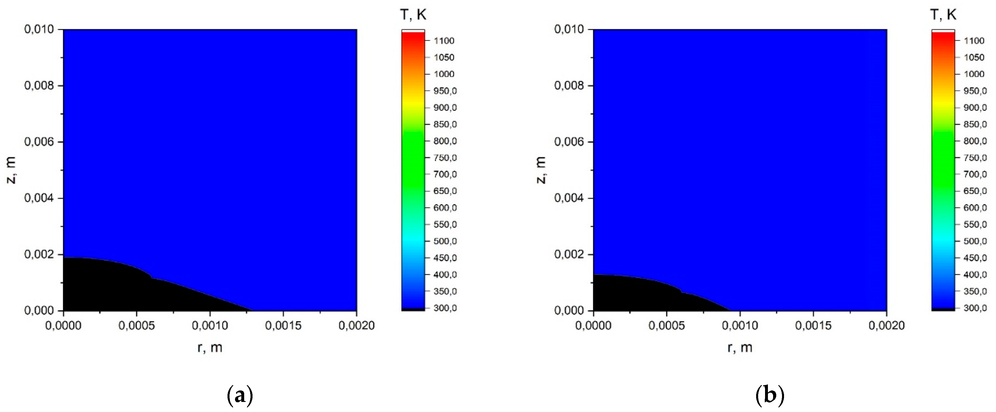
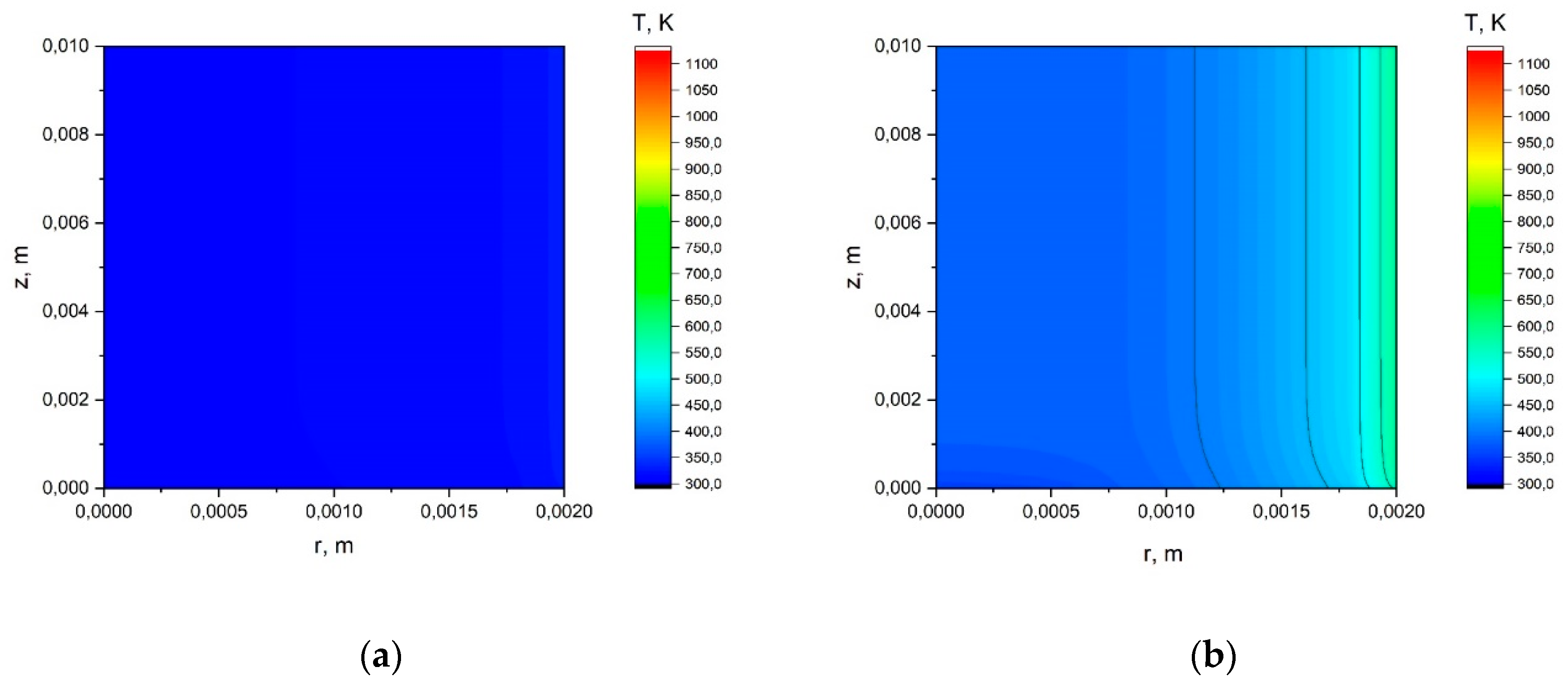
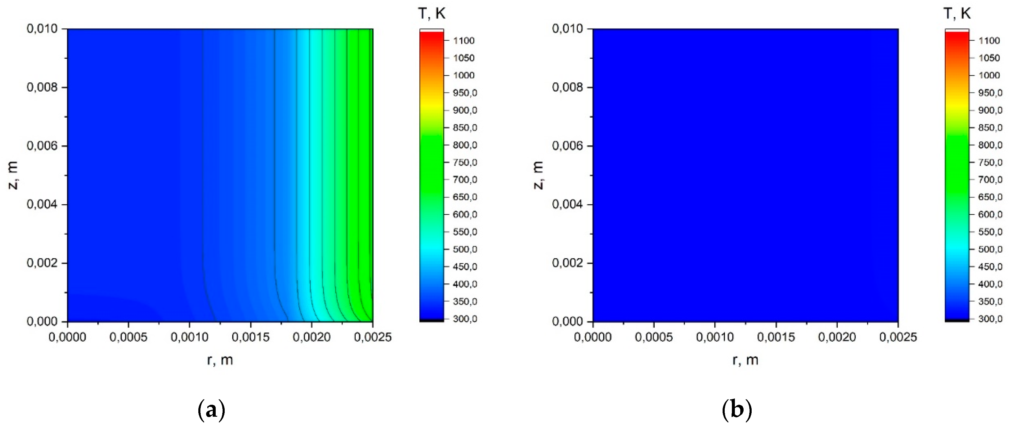
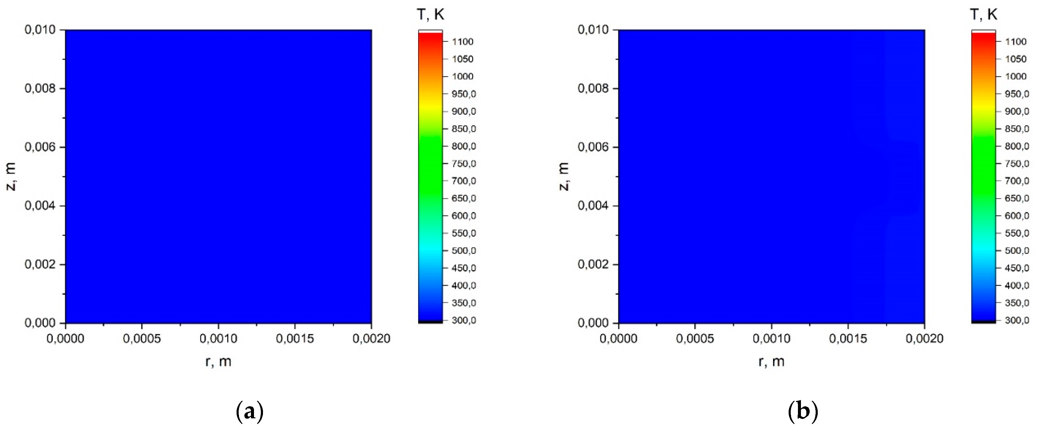
Figure A1.
Temperature distribution in the stem of a herbaceous plant: R = 0.002 m, t = 0.5 s, q = 0.5 kW/m2 (a); R = 0.002 m, t = 0.5 s, q = 3 kW/m2 (b).
Figure A1.
Temperature distribution in the stem of a herbaceous plant: R = 0.002 m, t = 0.5 s, q = 0.5 kW/m2 (a); R = 0.002 m, t = 0.5 s, q = 3 kW/m2 (b).

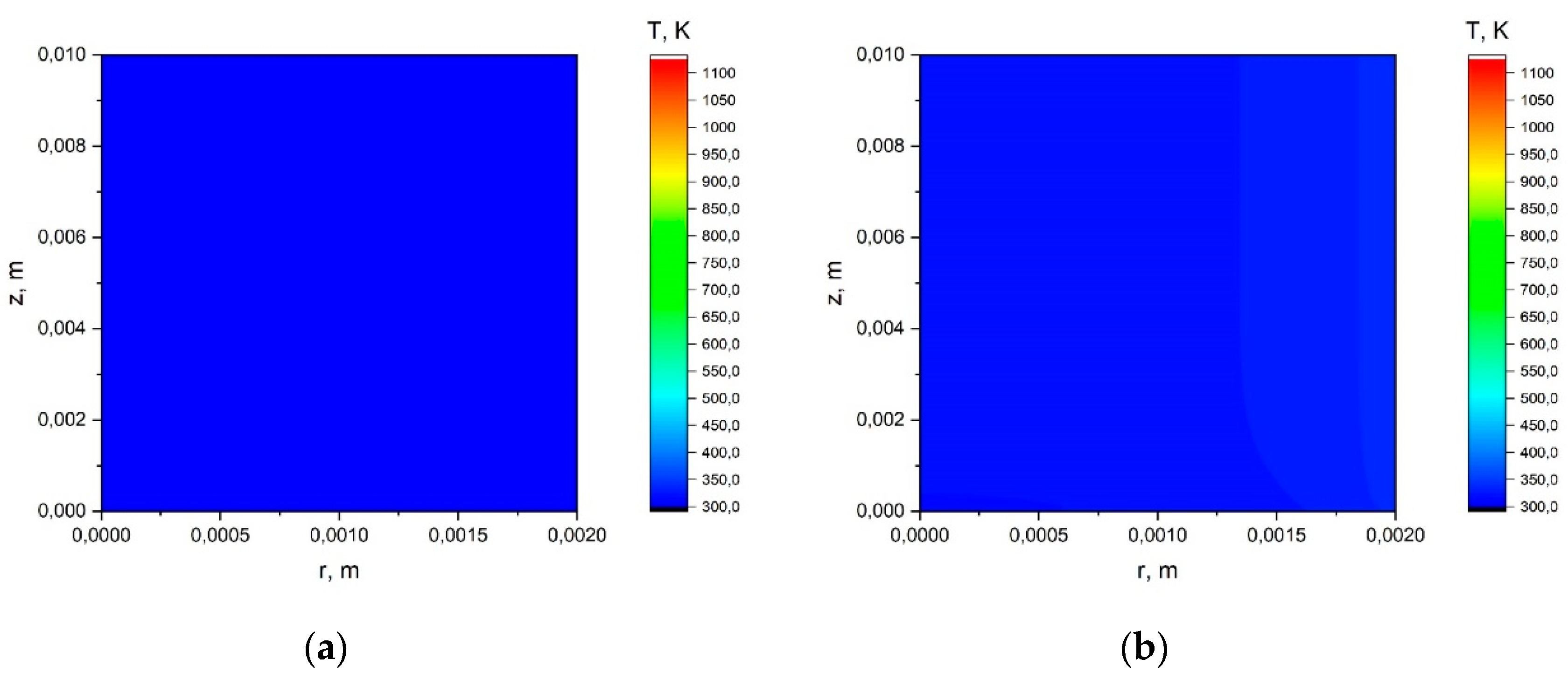
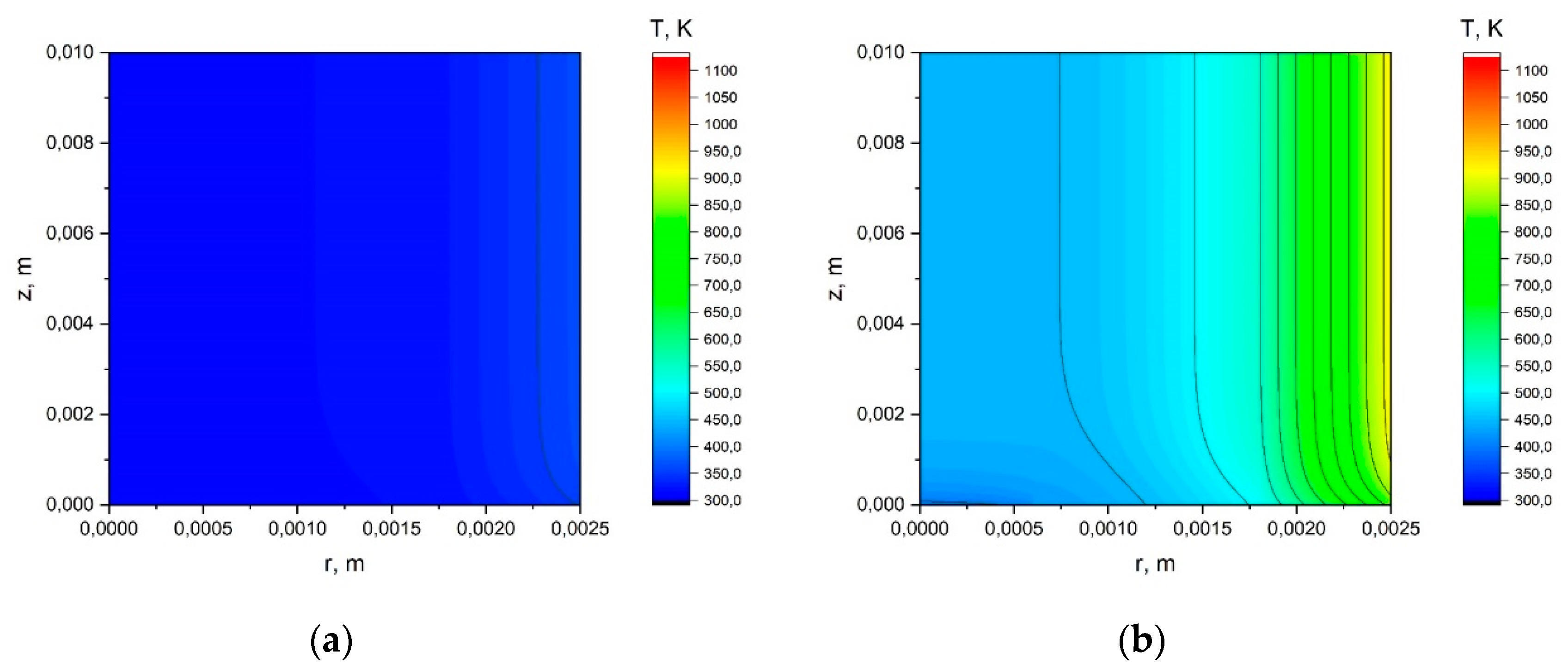
Figure A2.
Temperature distribution in the stem of a herbaceous plant: R = 0.002 m, t = 0.5 s, q = 30 kW/m2 (a); R = 0.002 m, t = 3 s, q = 0.5 kW/m2 (b).
Figure A2.
Temperature distribution in the stem of a herbaceous plant: R = 0.002 m, t = 0.5 s, q = 30 kW/m2 (a); R = 0.002 m, t = 3 s, q = 0.5 kW/m2 (b).
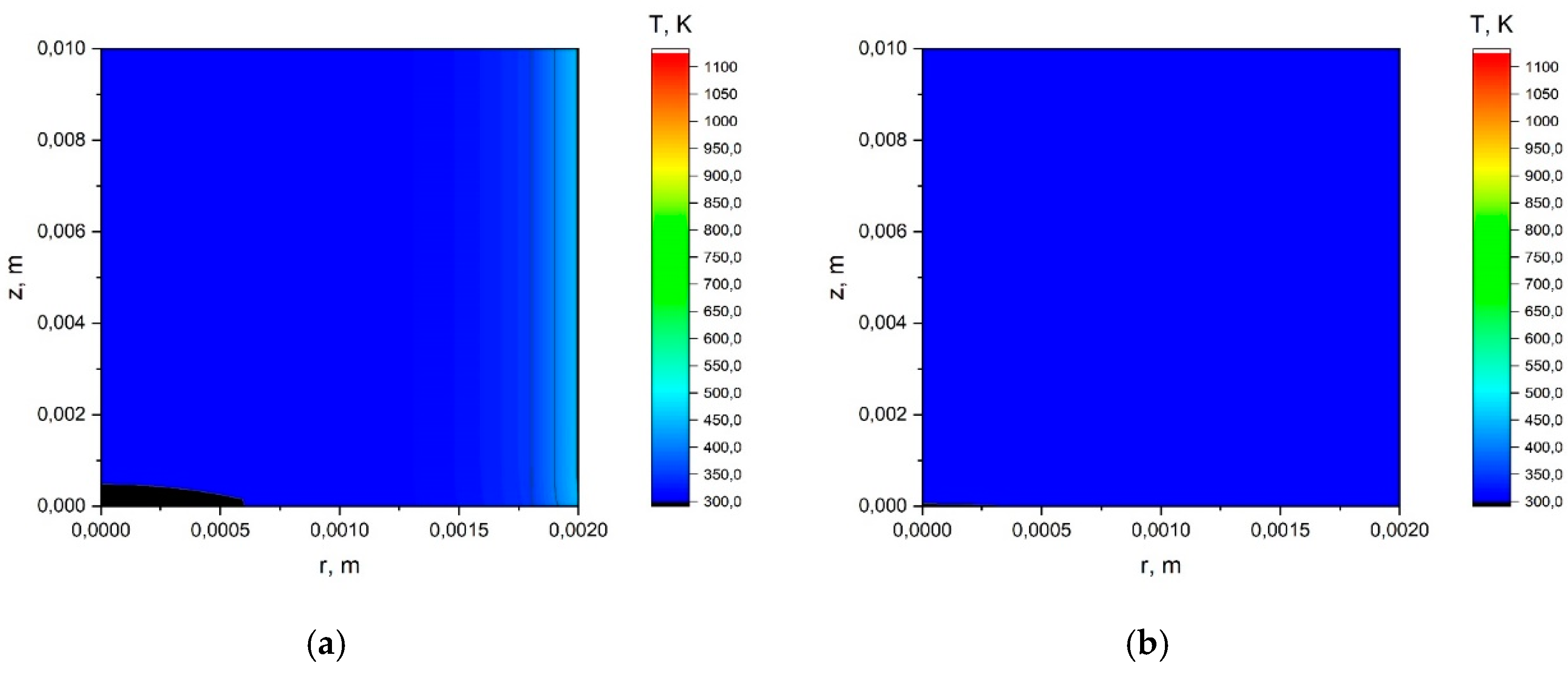
Figure A3.
Temperature distribution in the stem of a herbaceous plant: R = 0.002 m, t = 3 s, q = 3 kW/m2 (a); R = 0.002 m, t = 3 s, q = 30 kW/m2 (b).
Figure A3.
Temperature distribution in the stem of a herbaceous plant: R = 0.002 m, t = 3 s, q = 3 kW/m2 (a); R = 0.002 m, t = 3 s, q = 30 kW/m2 (b).

Figure A4.
Temperature distribution in the stem of a herbaceous plant: R = 0.002 m, t = 6 s, q = 0.5 kW/m2 (a); R = 0.002 m, t = 6 s, q = 3 kW/m2 (b).
Figure A4.
Temperature distribution in the stem of a herbaceous plant: R = 0.002 m, t = 6 s, q = 0.5 kW/m2 (a); R = 0.002 m, t = 6 s, q = 3 kW/m2 (b).

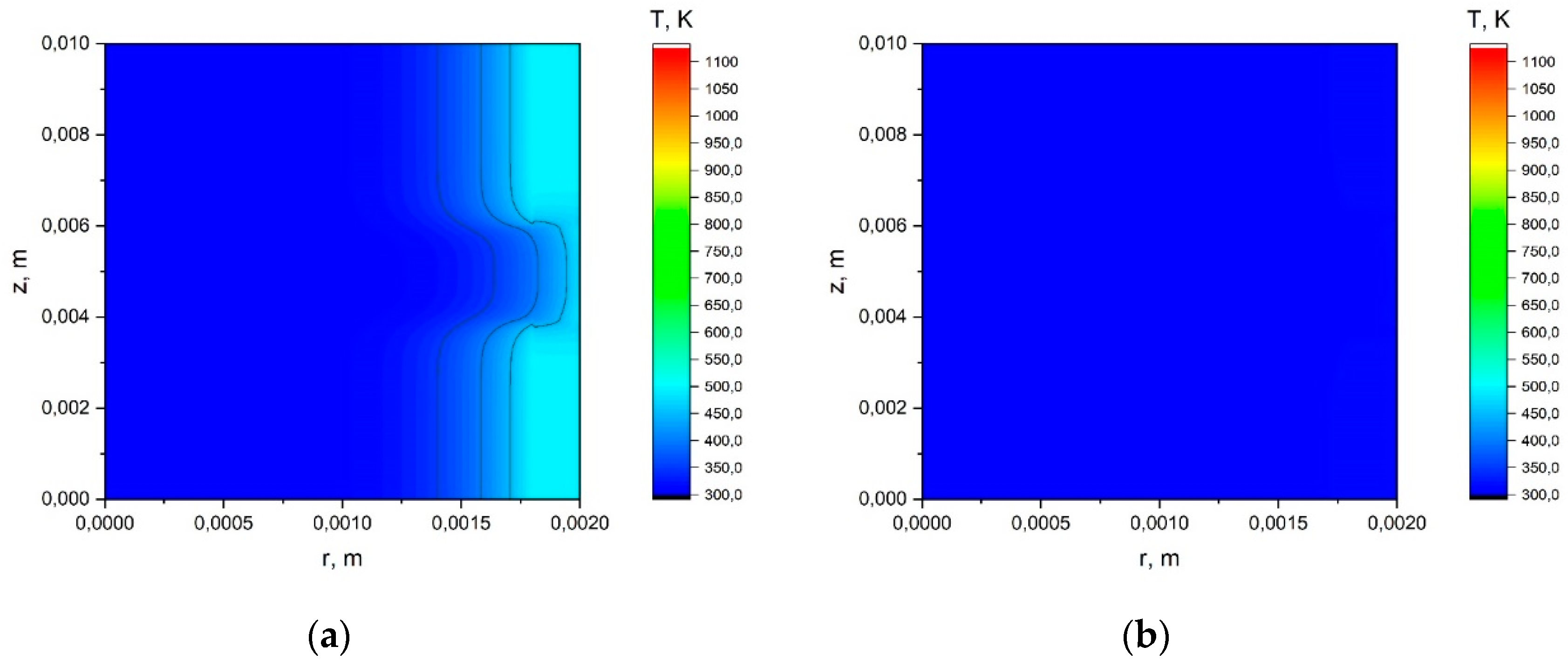
Figure A5.
Temperature distribution in the stem of a herbaceous plant: R = 0.002 m, t = 6 s, q = 30 kW/m2 (a); R = 0.0025 m, t = 0.5 s, q = 0.5 kW/m2 (b).
Figure A5.
Temperature distribution in the stem of a herbaceous plant: R = 0.002 m, t = 6 s, q = 30 kW/m2 (a); R = 0.0025 m, t = 0.5 s, q = 0.5 kW/m2 (b).

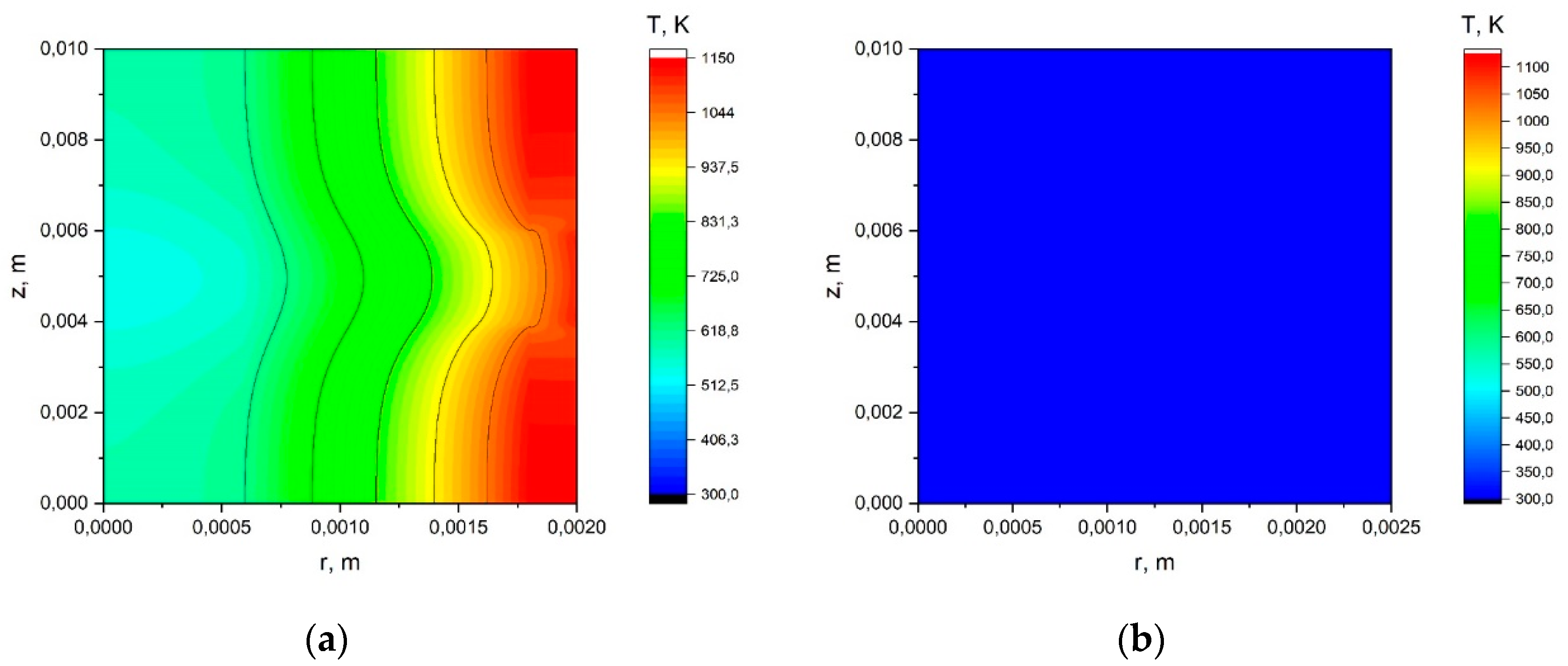
Figure A6.
Temperature distribution in the stem of a herbaceous plant: R = 0.0025 m, t = 0.5 s, q = 3 kW/m2 (a); R = 0.0025 m, t = 0.5 s, q = 30 kW/m2 (b).
Figure A6.
Temperature distribution in the stem of a herbaceous plant: R = 0.0025 m, t = 0.5 s, q = 3 kW/m2 (a); R = 0.0025 m, t = 0.5 s, q = 30 kW/m2 (b).

Figure A7.
Temperature distribution in the stem of a herbaceous plant: R = 0.0025 m, t = 3 s, q = 0.5 kW/m2 (a); R = 0.0025 m, t = 3 s, q = 3 kW/m2 (b).
Figure A7.
Temperature distribution in the stem of a herbaceous plant: R = 0.0025 m, t = 3 s, q = 0.5 kW/m2 (a); R = 0.0025 m, t = 3 s, q = 3 kW/m2 (b).

Figure A8.
Temperature distribution in the stem of a herbaceous plant: R = 0.0025 m, t = 3 s, q = 30 kW/m2 (a); R = 0.0025 m, t = 6 s, q = 0.5 kW/m2 (b).
Figure A8.
Temperature distribution in the stem of a herbaceous plant: R = 0.0025 m, t = 3 s, q = 30 kW/m2 (a); R = 0.0025 m, t = 6 s, q = 0.5 kW/m2 (b).

Figure A9.
Temperature distribution in the stem of a herbaceous plant: R = 0.0025 m, t = 6 s, q = 3 kW/m2 (a); R = 0.0025 m, t = 6 s, q = 30 kW/m2 (b).
Figure A9.
Temperature distribution in the stem of a herbaceous plant: R = 0.0025 m, t = 6 s, q = 3 kW/m2 (a); R = 0.0025 m, t = 6 s, q = 30 kW/m2 (b).

Figure A10.
Temperature distribution in the stem of a herbaceous plant: R = 0.003 m, t = 0.5 s, q = 0.5 kW/m2 (a); R = 0.003 m, t = 0.5 s, q = 3 kW/m2 (b).
Figure A10.
Temperature distribution in the stem of a herbaceous plant: R = 0.003 m, t = 0.5 s, q = 0.5 kW/m2 (a); R = 0.003 m, t = 0.5 s, q = 3 kW/m2 (b).
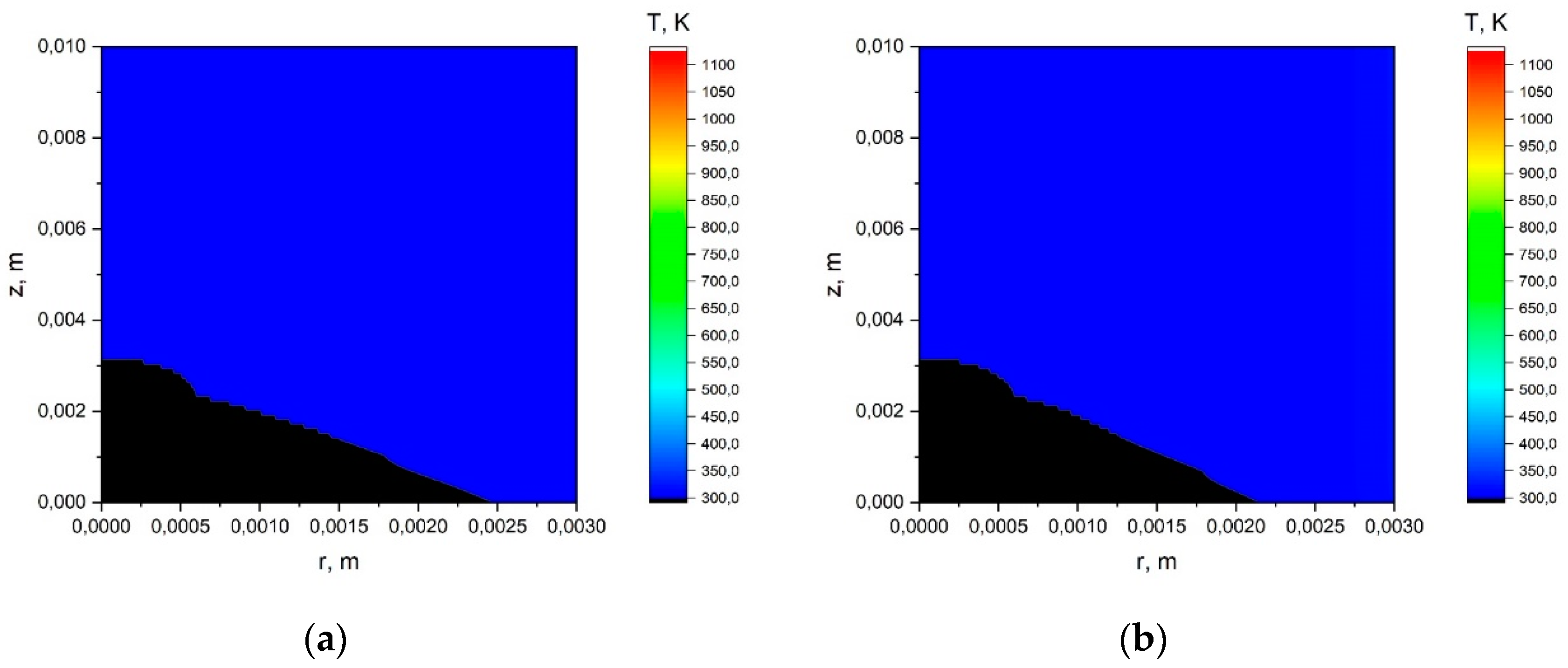
Figure A11.
Temperature distribution in the stem of a herbaceous plant: R = 0.003 m, t = 0.5 s, q = 30 kW/m2 (a); R = 0.003 m, t = 3 s, q = 0.5 kW/m2 (b).
Figure A11.
Temperature distribution in the stem of a herbaceous plant: R = 0.003 m, t = 0.5 s, q = 30 kW/m2 (a); R = 0.003 m, t = 3 s, q = 0.5 kW/m2 (b).

Figure A12.
Temperature distribution in the stem of a herbaceous plant: R = 0.003 m, t = 3 s, q = 3 kW/m2 (a); R = 0.003 m, t = 3 s, q = 30 kW/m2 (b).
Figure A12.
Temperature distribution in the stem of a herbaceous plant: R = 0.003 m, t = 3 s, q = 3 kW/m2 (a); R = 0.003 m, t = 3 s, q = 30 kW/m2 (b).
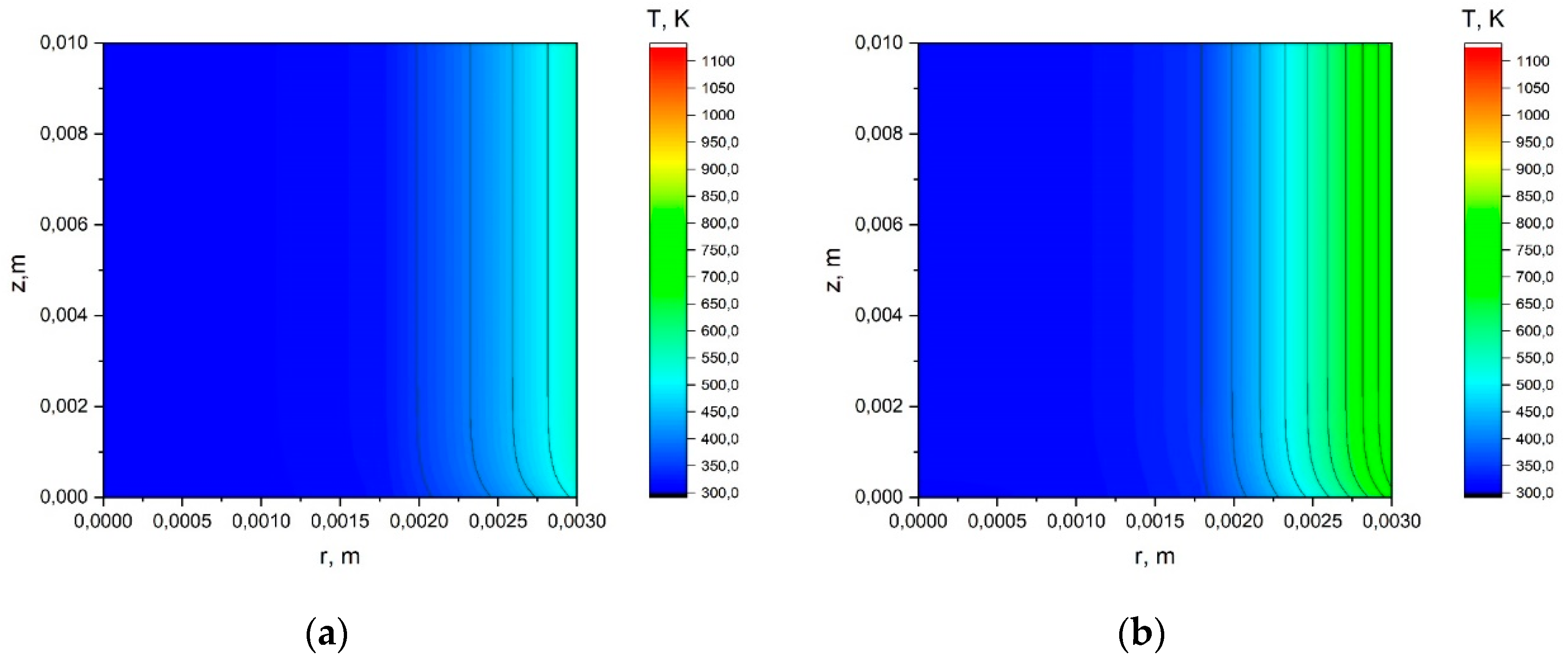
Figure A13.
Temperature distribution in the stem of a herbaceous plant: R = 0.003 m, t = 6 s, q = 0.5 kW/m2 (a); R = 0.003 m, t = 6 s, q = 3 kW/m2 (b).
Figure A13.
Temperature distribution in the stem of a herbaceous plant: R = 0.003 m, t = 6 s, q = 0.5 kW/m2 (a); R = 0.003 m, t = 6 s, q = 3 kW/m2 (b).

Figure A14.
Temperature distribution in the stem of a herbaceous plant: R = 0.003 m, t = 6 s, q = 30 kW/m2.
Figure A14.
Temperature distribution in the stem of a herbaceous plant: R = 0.003 m, t = 6 s, q = 30 kW/m2.

Appendix A.2. The Results of the Calculation Using the Model with a Joint
This section presents the results of a numerical study of the mathematical model of heat transfer in the stem, taking into account the joint, under the influence of radiation from a surface forest fire. Figure A15, Figure A16, Figure A17, Figure A18, Figure A19, Figure A20, Figure A21, Figure A22, Figure A23, Figure A24, Figure A25, Figure A26, Figure A27 and Figure A28 show the temperature distribution for individual scenarios of the impact of the surface forest fire on the stem of a herbaceous plant.
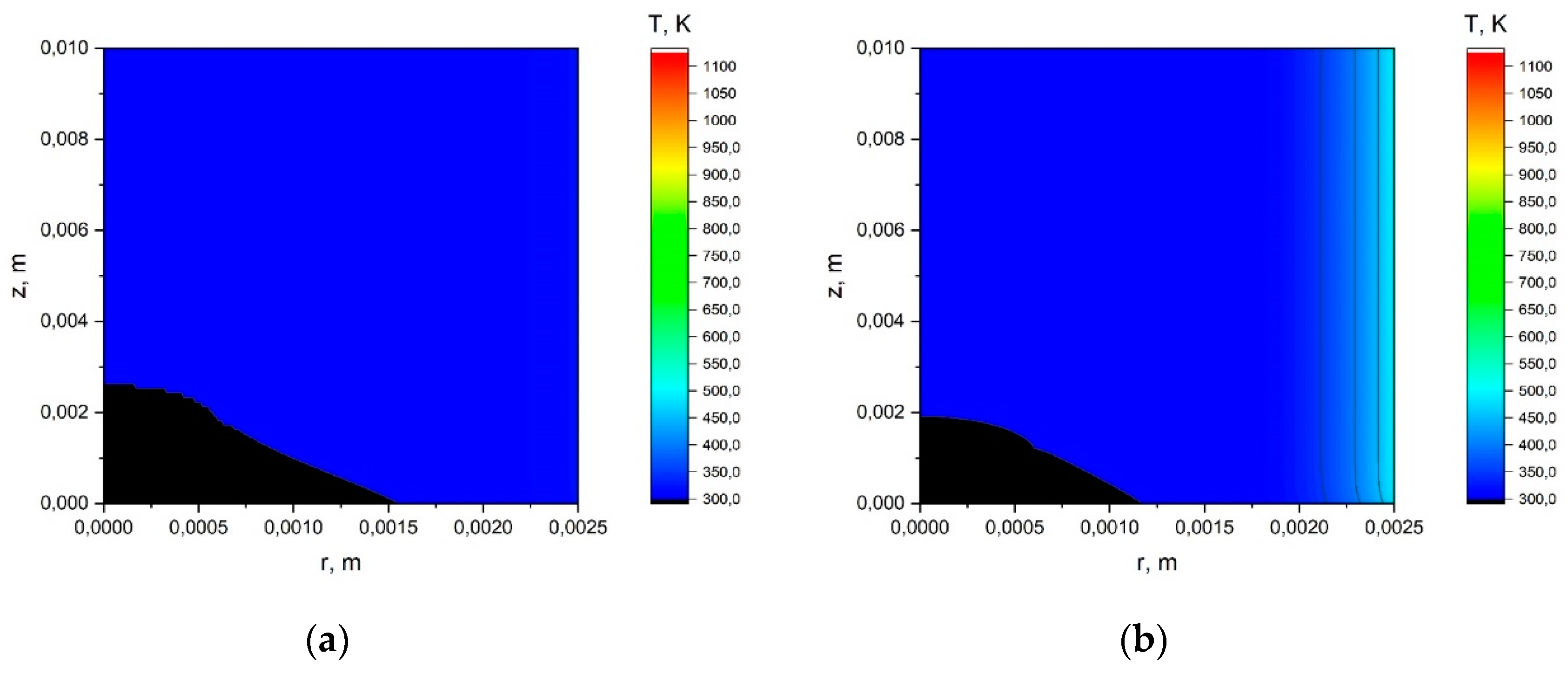
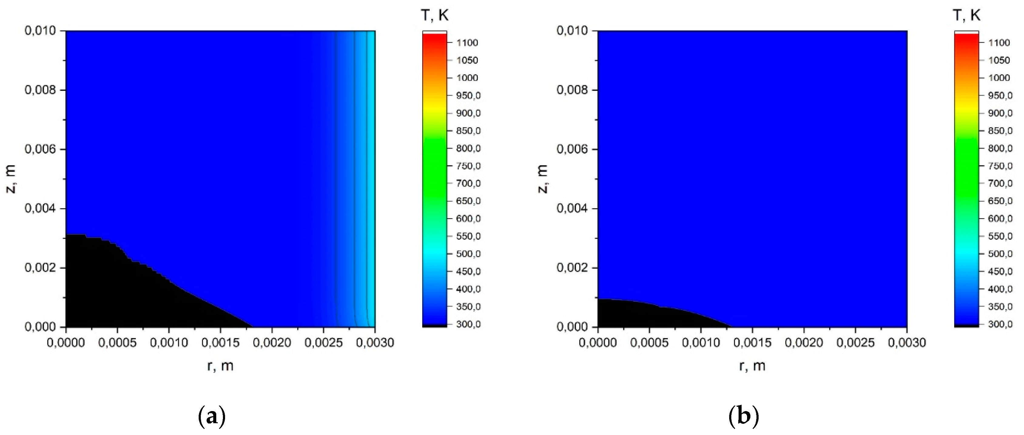
Figure A15.
Temperature distribution in the stem of a herbaceous plant: R = 0.002 m, t = 0.5 s, q = 0.5 kW/m2 (a); R = 0.002 m, t = 0.5 s, q = 3 kW/m2 (b).
Figure A15.
Temperature distribution in the stem of a herbaceous plant: R = 0.002 m, t = 0.5 s, q = 0.5 kW/m2 (a); R = 0.002 m, t = 0.5 s, q = 3 kW/m2 (b).

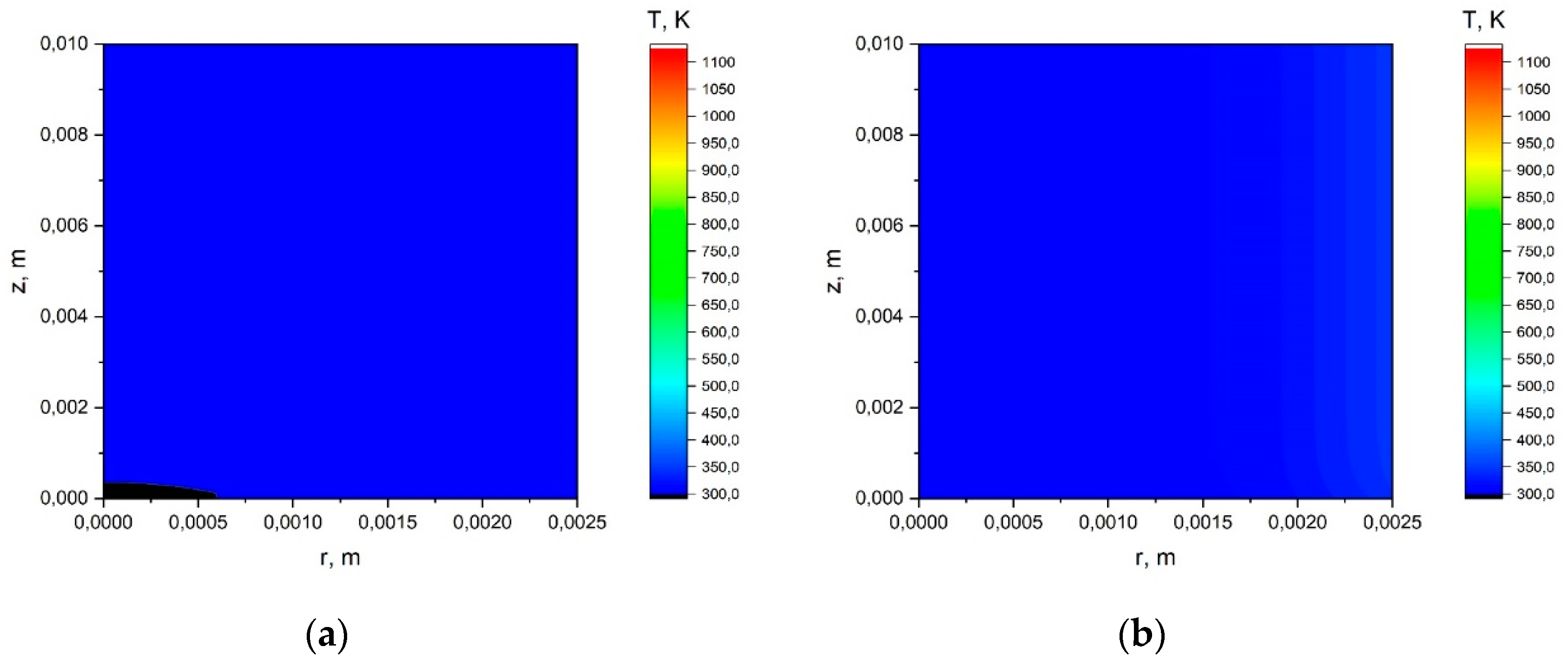
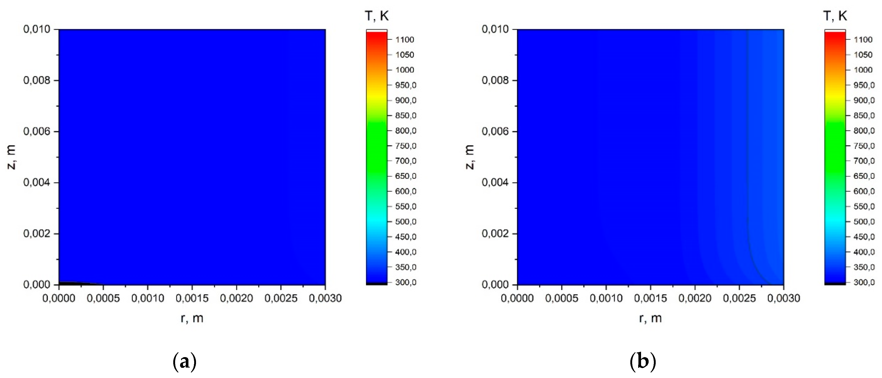
Figure A16.
Temperature distribution in the stem of a herbaceous plant: R = 0.002 m, t = 0.5 s, q = 30 kW/m2 (a); R = 0.002 m, t = 3 s, q = 0.5 kW/m2 (b).
Figure A16.
Temperature distribution in the stem of a herbaceous plant: R = 0.002 m, t = 0.5 s, q = 30 kW/m2 (a); R = 0.002 m, t = 3 s, q = 0.5 kW/m2 (b).

Figure A17.
Temperature distribution in the stem of a herbaceous plant: R = 0.002 m, t = 3 s, q = 3 kW/m2 (a); R = 0.002 m, t = 3 s, q = 30 kW/m2 (b).
Figure A17.
Temperature distribution in the stem of a herbaceous plant: R = 0.002 m, t = 3 s, q = 3 kW/m2 (a); R = 0.002 m, t = 3 s, q = 30 kW/m2 (b).
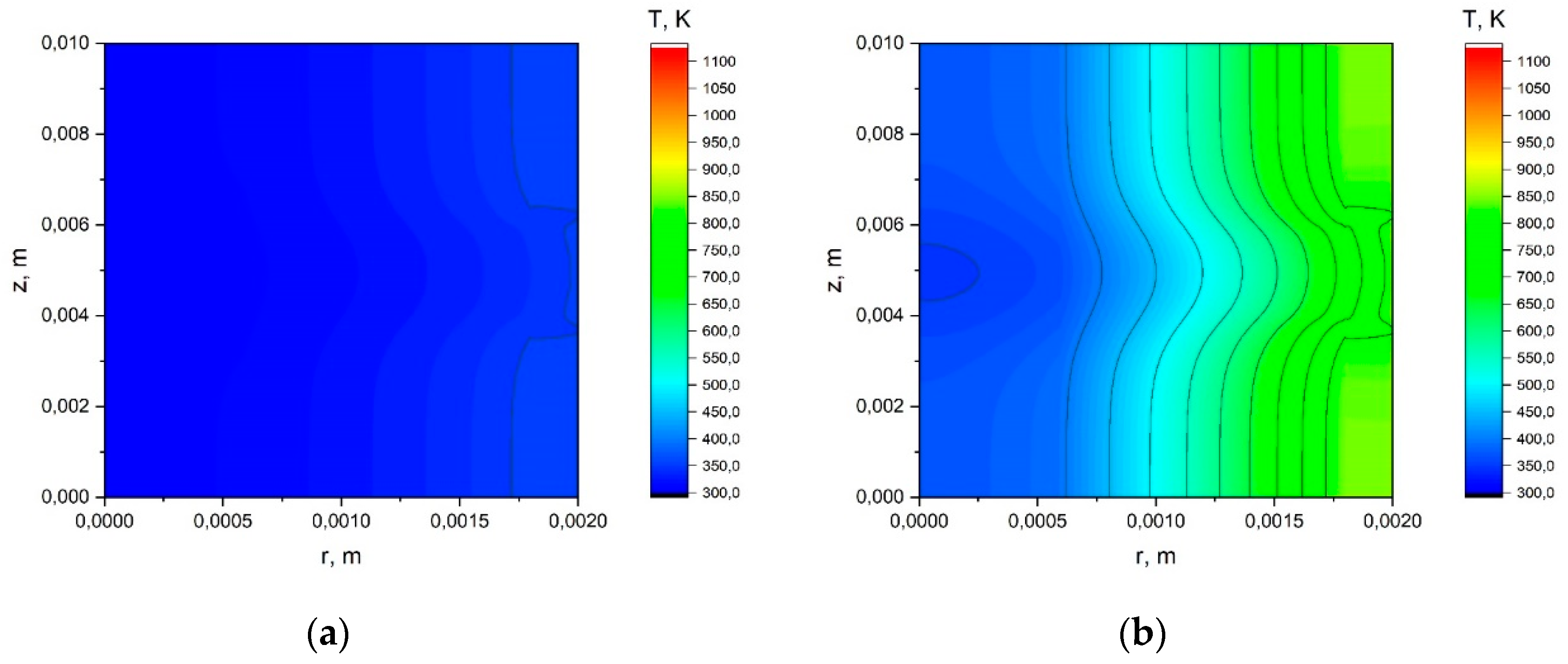
Figure A18.
Temperature distribution in the stem of a herbaceous plant: R = 0.002 m, t = 6 s, q = 0.5 kW/m2 (a); R = 0.002 m, t = 6 s, q = 3 kW/m2 (b).
Figure A18.
Temperature distribution in the stem of a herbaceous plant: R = 0.002 m, t = 6 s, q = 0.5 kW/m2 (a); R = 0.002 m, t = 6 s, q = 3 kW/m2 (b).

Figure A19.
Temperature distribution in the stem of a herbaceous plant: R = 0.002 m, t = 6 s, q = 30 kW/m2 (a); R = 0.0025 m, t = 0.5 s, q = 0.5 kW/m2 (b).
Figure A19.
Temperature distribution in the stem of a herbaceous plant: R = 0.002 m, t = 6 s, q = 30 kW/m2 (a); R = 0.0025 m, t = 0.5 s, q = 0.5 kW/m2 (b).

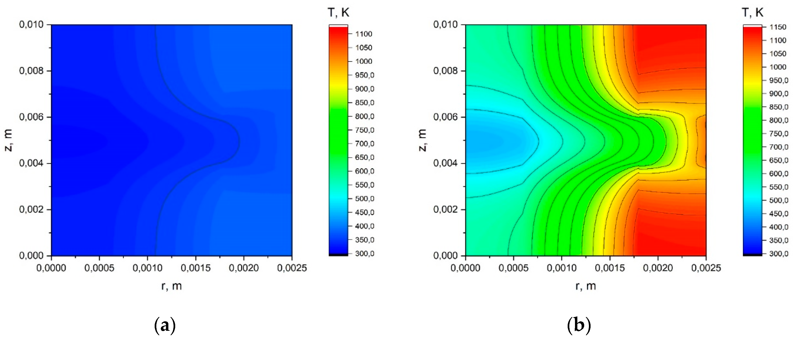
Figure A20.
Temperature distribution in the stem of a herbaceous plant: R = 0.0025 m, t = 0.5 s, q = 3 kW/m2 (a); R = 0.0025 m, t = 0.5 s, q = 30 kW/m2 (b).
Figure A20.
Temperature distribution in the stem of a herbaceous plant: R = 0.0025 m, t = 0.5 s, q = 3 kW/m2 (a); R = 0.0025 m, t = 0.5 s, q = 30 kW/m2 (b).

Figure A21.
Temperature distribution in the stem of a herbaceous plant: R = 0.0025 m, t = 3 s, q = 0.5 kW/m2 (a); R = 0.0025 m, t = 3 s, q = 3 kW/m2 (b).
Figure A21.
Temperature distribution in the stem of a herbaceous plant: R = 0.0025 m, t = 3 s, q = 0.5 kW/m2 (a); R = 0.0025 m, t = 3 s, q = 3 kW/m2 (b).

Figure A22.
Temperature distribution in the stem of a herbaceous plant: R = 0.0025 m, t = 3 s, q = 30kW/m2 (a); R = 0.0025 m, t = 6 s, q = 0.5 kW/m2 (b).
Figure A22.
Temperature distribution in the stem of a herbaceous plant: R = 0.0025 m, t = 3 s, q = 30kW/m2 (a); R = 0.0025 m, t = 6 s, q = 0.5 kW/m2 (b).
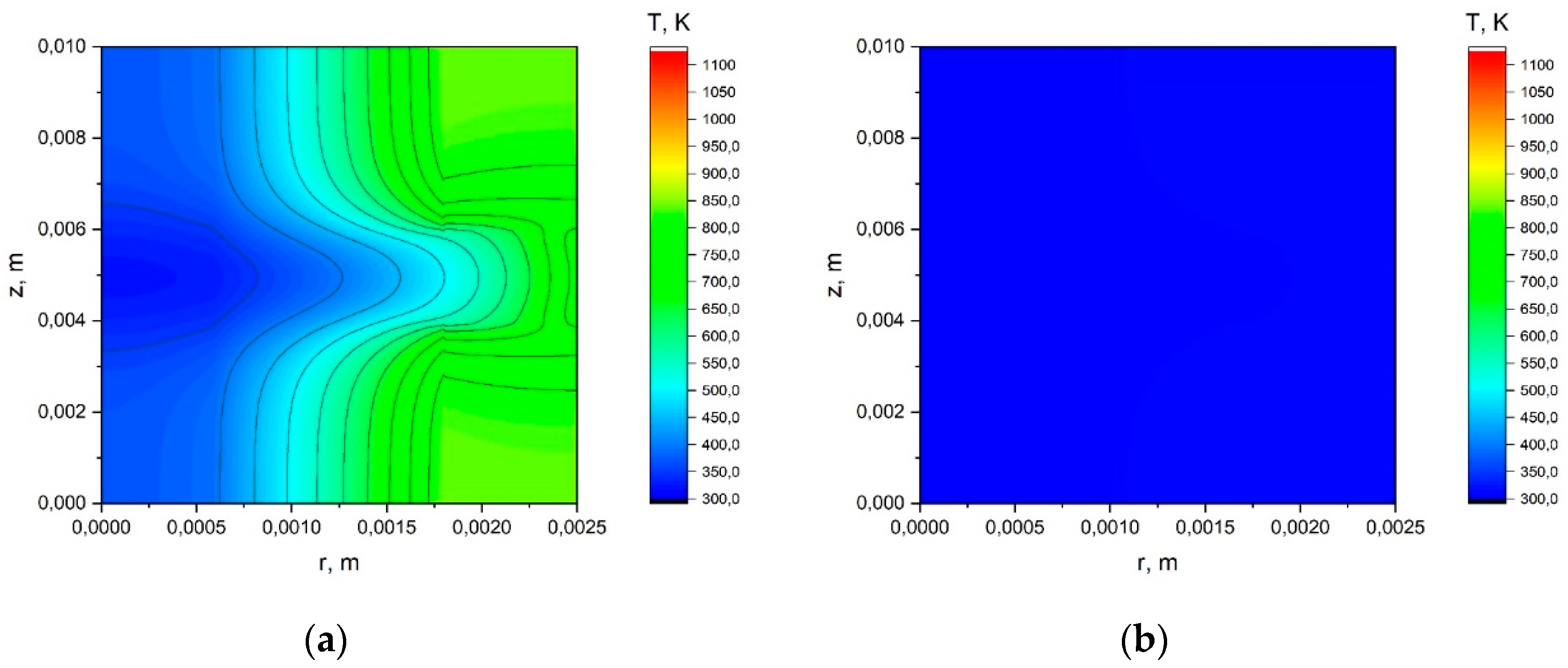
Figure A23.
Temperature distribution in the stem of a herbaceous plant: R = 0.0025 m, t = 6 s, q = 3 kW/m2 (a); R = 0.0025 m, t = 6 s, q = 30 kW/m2 (b).
Figure A23.
Temperature distribution in the stem of a herbaceous plant: R = 0.0025 m, t = 6 s, q = 3 kW/m2 (a); R = 0.0025 m, t = 6 s, q = 30 kW/m2 (b).

Figure A24.
Temperature distribution in the stem of a herbaceous plant: R = 0.003 m, t = 0.5 s, q = 0.5 kW/m2 (a); R = 0.003 m, t = 0.5 s, q = 3 kW/m2 (b).
Figure A24.
Temperature distribution in the stem of a herbaceous plant: R = 0.003 m, t = 0.5 s, q = 0.5 kW/m2 (a); R = 0.003 m, t = 0.5 s, q = 3 kW/m2 (b).
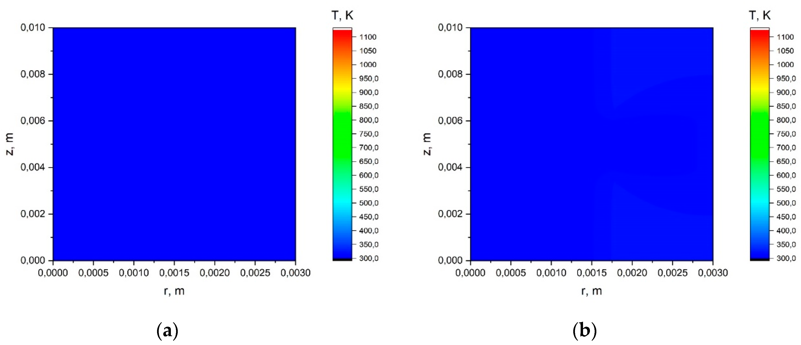
Figure A25.
Temperature distribution in the stem of a herbaceous plant: R = 0.003 m, t = 0.5 s, q = 30 kW/m2 (a); R = 0.003 m, t = 3 s, q = 0.5 kW/m2 (b).
Figure A25.
Temperature distribution in the stem of a herbaceous plant: R = 0.003 m, t = 0.5 s, q = 30 kW/m2 (a); R = 0.003 m, t = 3 s, q = 0.5 kW/m2 (b).
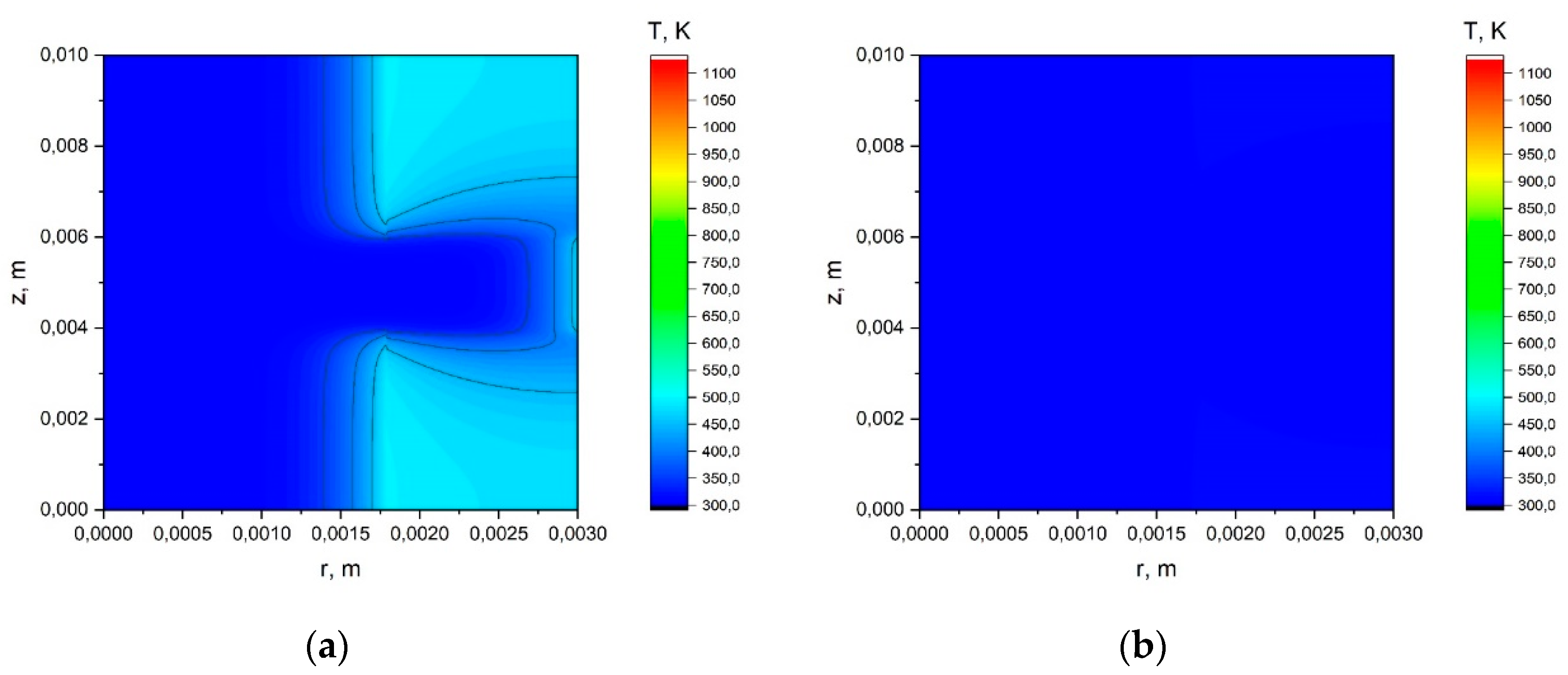
Figure A26.
Temperature distribution in the stem of a herbaceous plant: R = 0.003 m, t = 3 s, q = 3 kW/m2 (a); R = 0.003 m, t = 3 s, q = 30 kW/m2 (b).
Figure A26.
Temperature distribution in the stem of a herbaceous plant: R = 0.003 m, t = 3 s, q = 3 kW/m2 (a); R = 0.003 m, t = 3 s, q = 30 kW/m2 (b).

Figure A27.
Temperature distribution in the stem of a herbaceous plant: R = 0.003 m, t = 6 s, q = 0.5 kW/m2 (a); R = 0.003 m, t = 6 s, q = 3 kW/m2 (b).
Figure A27.
Temperature distribution in the stem of a herbaceous plant: R = 0.003 m, t = 6 s, q = 0.5 kW/m2 (a); R = 0.003 m, t = 6 s, q = 3 kW/m2 (b).

Figure A28.
Temperature distribution in the stem of a herbaceous plant: R = 0.003 m, t = 6 s, q = 30 kW/m2.
Figure A28.
Temperature distribution in the stem of a herbaceous plant: R = 0.003 m, t = 6 s, q = 30 kW/m2.

References
- Volokitina, A.V.; Sofronov, M.A. Classification and Mapping of Plant Combustible Materials; Publishing House of the Siberian Branch of the Russian Academy of Sciences: Novosibirsk, Russia, 2002; p. 314. [Google Scholar]
- Baranovskiy, N.V.; Demikhova, A.N. Mathematical Model of Heat Transfer in Morphological Part of Vegetation at Influence by Thermal Radiation from Surface Forest Fire Front. MATEC Web Conf. 2016, 72, 01025. [Google Scholar] [CrossRef] [Green Version]
- Esau, K. Anatomy of Seed Plants, 2nd ed.; Wiley: New York, NY, USA, 1977. [Google Scholar]
- Grishin, A.M. Mathematical Modeling of Forest Fire and New Methods of Fighting Them; Publishing House of the Tomsk State University: Tomsk, Russia, 1997; p. 390. [Google Scholar]
- Perminov, V.; Soprunenko, E. Numerical solution of crown forest fire initiation and spread problem. In Proceedings of the 2016 11th International Forum on Strategic Technology, IFOST, Novosibirsk, Russia, 1–3 June 2016; pp. 400–404. [Google Scholar] [CrossRef]
- Valette, J.-C.; Gomendy, V.; Houssard, C.; Gillon, D. Heat transfer in the soil during very low-intensity experimantal fires—The role of duff and soil-moisture content. Int. J. Wildland Fire 1994, 4, 225. [Google Scholar] [CrossRef]
- Scotter, D.R. Soil temperature under grass fires. Aust. J. Soil Res. 1970, 8, 273–279. [Google Scholar] [CrossRef]
- Stoof, C.R. Soil heating. In Fire Effects on Soil Properties; CSIRO Publishing: Clayton South, Australia, 2019; pp. 229–240. [Google Scholar]
- Pereira, P.; Úbeda, X.; Francos, M. Laboratory fire simulations: Plant litter and soils. In Fire Effects on Soil Properties; CSIRO Publishing: Clayton South, Australia, 2019; pp. 15–38. [Google Scholar]
- Redmann, R.E. Nitrogen losses to the atmosphere from grassland fires in Saskatchewan, Canada. Int. J. Wildland Fire 1991, 1, 239–244. [Google Scholar] [CrossRef]
- Strand, T.; Gullett, B.; Urbanski, S.; O’Neil, S.; Potter, B.; Aurell, J.; Holder, A.; Larkin, N.; Moore, M.; Rorig, M. Grassland and forest understorey biomass emissions from prescribed fires in the southeastern United States—RxCADRE 2012. Int. J. Wildland Fire 2016, 25, 102–113. [Google Scholar] [CrossRef]
- Wang, S.; Ali Baig, M.H.; Liu, S.; Wan, H.; Wu, T.; Yang, Y. Estimating the area burned by agricultural fires from Landsat 8 data using the Vegetation Difference Index and Burn Scar Index. Int. J. Wildland Fire 2018, 27, 217–227. [Google Scholar] [CrossRef]
- Kurbatsky, N.P. Terminology of forest pyrology. In Questions of forest pyrology; ILID SB AS USSR: Krasnoyarsk, Russia, 1972; pp. 171–231. [Google Scholar]
- Baranovskiy, N.V.; Kuznetsov, G.V. Forest Fire Occurrences and Ecological Impact Prediction: Monograph; Publishing House of the Siberian Branch of the Russian Academy of Science: Novosibirsk, Russia, 2017. [Google Scholar]
- Kipfmueller, K.; Elizabeth, A.; Schneider, S.A.; Weyenberg, L.B.; Johnson, G. Historical drivers of the frequent fire regime in the red pine forests of Voyageurs National Park, MN, USA. For. Ecol. Manag. 2017, 405, 31–43. [Google Scholar] [CrossRef]
- Baranovskiy, N.V.; Kuznetsov, G.V. Coniferous tree ignition by cloud-to-ground lightning discharge using approximation of “ideal” crack in bark. JP J. Heat Mass Transf. 2017, 14, 173–186. [Google Scholar] [CrossRef]
- Vorobiev, Y.L. Forest fires on the territory of Russia: Status and problems. Ecol. J. 2009, 3, 9–11. [Google Scholar]
- Amatulli, G.; Perez-Cabello, F.; Du la Riva, J. Mapping lightning/human-caused wildfires occurrence under ignition point location uncertainty. Ecol. Model. 2007, 200, 321–333. [Google Scholar] [CrossRef]
- Clarke, H.; Tran, B.; Boer, M.M.; Price, O.; Kenny, B.; Bradstock, R. Climate change effects on the frequency, seasonality and interannual variability of suitable prescribed burning weather conditions in south-eastern Australia. Agric. For. Meteorol. 2019, 271, 148–157. [Google Scholar] [CrossRef]
- Ilina, V.P. Pyrogenic effect on vegetation cover. Samara Luka: Problems of regional and global ecology. 2011, 20, 4–30. [Google Scholar]
- Bryukhanov, A.V. Environmental assessment of the state of forests in Siberia. Sustain. For. Manag. 2009, 2, 21–31. [Google Scholar]
- Staggs, J.E.J. A simple model of polymer pyrolysis including transport of volatiles. Fire Saf. J. 2000, 34, 69–80. [Google Scholar] [CrossRef]
- Di Blasi, C. Modelling and simulation of combustion processes of charring and non-charring solid fuels. Prog. Energy Combust. Sci. 1993, 19, 71–104. [Google Scholar] [CrossRef]
- Carlslaw, S.; Jaeger, J.C. Conduction of Heat in Solids; Oxford University Press: Oxford, UK, 1984; p. 510. [Google Scholar]
- Landau, G. Heat conduction in a melting solid. Q. J. Appl. Math. 1950, 8, 81–94. [Google Scholar] [CrossRef] [Green Version]
- Billings, M.J.; Warren, L.; Wilkins, R. Thermal erosion of electrical insulating materials. IEEE Trans. Electr. Insulation 1971, 6, 82–90. [Google Scholar] [CrossRef]
- Whiting, P.; Dowden, J.M.; Kapadia, P.D.; Davis, M.P. A one-dimensional mathematical model of laser induced thermal ablation of biological tissue. Lasers Med. Sci. 1992, 7, 357–368. [Google Scholar] [CrossRef]
- Kindelan, M.; Williams, F.A. Theory for endothermic gasification of a solid by a constant energy flux. Combust. Sci. Technol. 1975, 10, 1–9. [Google Scholar] [CrossRef]
- Wichman, I.S. A model describing the steady-state gasification of bubble-forming thermoplastics in response to an incident heat flux. Combust. Flame 1986, 63, 217–229. [Google Scholar] [CrossRef]
- Spearpoint, M.J.; Quintiere, J.G. Predicting the piloted ignition of wood in the cone calorimeter using an integral model—Effect of species, grain orientation and heat flux. Fire Saf. J. 2001, 36, 391–415. [Google Scholar] [CrossRef]
- Mackay, G.D.M. Mechanism of Thermal Degradation of Cellulose: A Review of the Literature; Forestry Branch Departmental Publication no 1201; Canada Department of Forestry and Rural Development: Petawawa, ON, Canada, 1967; p. 2. [Google Scholar]
- Moghtaderi, B. The state-of-the-art in pyrolysis modeling of lignocellulosic solid fuels. Fire Mater. 2006, 30, 1–34. [Google Scholar] [CrossRef]
- Galgano, A.; Di Blasi, C. Modeling the propagation of drying and decomposition fronts in wood. Combust. Flame 2004, 139, 16–27. [Google Scholar] [CrossRef]
- Shen, D.K.; Fang, M.X.; Luo, Z.Y.; Cen, K.F. Modeling pyrolysis of wet wood under external heat flux. Fire Saf. J. 2007, 42, 210–217. [Google Scholar] [CrossRef]
- Cruz, M.G.; Sullivan, A.L.; Gould, J.S.; Hurley, R.J.; Plucinski, M.P. Got to burn to learn: The effect of fuel load on grassland fire behavior and its management implications. Int. J. Wildland Fire 2018, 27, 727–741. [Google Scholar] [CrossRef]
- Deeming, J.E.; Burgan, R.E.; Cohen, J.D. The National Fire Danger Rating System—1978; General Technical Report INT—39; USDA Forest Service, Intermountain Forest and Range Experimental Station: Odgen, UT, USA, 1977. [Google Scholar]
- Alexander, M.E. Proposed Revision of Fire Danger Class Criteria for Forest and Rural Areas in New Zeland; National Rural Fire Authority: Wellington, New Zeland, 2008. [Google Scholar]
- Byram, G.M. Combustion of Forest Fuels//In Forest Fire: Control and Use; Davis, K.P., Ed.; McGraw-Hill: New York, NY, USA, 1959. [Google Scholar]
- Rothermel, R.C. A Mathematical Model for Predicting Fire Spread in Wildland Fuels; Research Paper INT-115; USDA Forest Service, Intermountain Forest and Range Experimental Station: Odgen, UT, USA, 1972. [Google Scholar]
- Luke, R.H.; McArthur, A.G. Bushfires in Australia; Australian Government Publishing Service: Canberra, Australia, 1978. [Google Scholar]
- Fernandes, P.M.; Botelho, H.S. A review of prescribed burning effectiveness in fire hazard reduction. Int. J. Wildland Fire 2003, 12, 117–128. [Google Scholar] [CrossRef] [Green Version]
- Fernandes, P.M. Empirical support for the use of prescribed burning as a fuel treatment. Curr. For. Rep. 2015, 1, 118–127. [Google Scholar] [CrossRef]
- Zhang, Z.; Zhang, H.; Feng, Z.; Li, X.; Bi, Y.; Shi, D.; Zhou, D.; Wang, Y.; Duwala; Zhao, J. A method for estimating the amount of dead grass fuel based on spectral reflectance characteristics. Int. J. Wildland Fire 2015, 24, 940–948. [Google Scholar] [CrossRef]
- Lu, B.; He, Y.; Tong, A. Evaluation of spectral indices for estimating burn severity in semiarid grasslands. Int. J. Wildland Fire 2016, 25, 147–157. [Google Scholar] [CrossRef]
- Martin, D.; Chen, T.; Nichols, D.; Bessell, R.; Kidnie, S.; Alexander, J. Integrating ground and satellite-based observations to determine the degree of grassland curing. Int. J. Wildland Fire 2015, 24, 329–339. [Google Scholar] [CrossRef]
- Dimitrakopoulos, A.P.; Mitsopoulos, I.D.; Gatoulas, K. Assessing ignition probability and moisture of extinction in a Mediterranean grass fuel. Int. J. Wildland Fire 2010, 19, 29–34. [Google Scholar] [CrossRef]
- Nelson, R.M., Jr. Water relations of forest fuels. In Forest Fires: Behavior and Ecological Effects; Johnson, E.A., Miyanishi, K., Eds.; Academic Press: Cambridge, CA, USA, 2001; pp. 79–150. [Google Scholar]
- Drysdale, D. An Introduction to Fire Dynamics; Wiley: Chichester, UK, 1998. [Google Scholar]
- Cheney, N.P.; Gould, J.S.; Catchpole, W.R. Prediction of fire spread in grasslands. Int. J. Wildland Fire 1998, 8, 1–13. [Google Scholar] [CrossRef]
- Mell, W.; Jenkins, M.A.; Gould, J.; Cheney, P. A physics-based approach to modeling grassland fires. Int. J. Wildland Fire 2007, 16, 1–22. [Google Scholar] [CrossRef]
- Cruz, M.G. Monte Carlo-based ensemble method for prediction of grassland fire spread. Int. J. Wildland Fire 2010, 19, 521–530. [Google Scholar] [CrossRef]
- Clements, C.B. Thermodynamic structure of a grass fire plume. Int. J. Wildland Fire 2010, 19, 895–902. [Google Scholar] [CrossRef]
- GEOPORTAL FGBU «ROSLESINFORG». Available online: http://geoportal.roslesinforg.ru:8080/ (accessed on 8 July 2019).
- Lesohozyaystvennyie Reglamentyi. Available online: http://egov-buryatia.ru/ralh/activities/documents/lesokhozyaystvennye-reglamenty/ (accessed on 8 July 2019).
- Official Site MO “Ivolginskiy Rayon”. Available online: http://egov-buryatia.ru/ivolga/o-munitsipalnom-obrazovanii/ob-organizatsii/ (accessed on 8 July 2019).
- Forest Resources. Available online: http://egov-buryatia.ru/about_republic/nature-resources/lesnye-resursy-/ (accessed on 9 July 2019).
- Yankovich, K.S.; Yankovich, E.P.; Baranovskiy, N.V. Classification of Vegetation to Estimate Forest Fire Danger Using Landsat 8 Images: Case Study. Math. Probl. Eng. 2019, 2019, 6296417. [Google Scholar] [CrossRef]
- Samarskii, A.A.; Vabishchevich, P.N. Computational Heat Transfer, Volume 1, Mathematical Modelling; Wiley: Chichester, UK, 1995. [Google Scholar]
- Samarskii, A.A.; Vabishchevich, P.N. Computational Heat Transfer, Volume 2, The Finite Difference Method; Wiley: Chichester, UK, 1995. [Google Scholar]
- Von Arx, G.; Crivellaro, A.; Prendin, A.L.; Čufar, K.; Carrer, M. Quantitative wood anatomy-practical guidelines. Front. Plant Sci. 2016, 7, 781. [Google Scholar] [CrossRef] [PubMed]
- Ward, D. Combustion chemistry and smoke. In Forest Fires: Behavior and Ecological Effects; Johnson, E.A., Miyanishi, K., Eds.; Academic Press: Cambridge, CA, USA, 2001; pp. 55–77. [Google Scholar]
- Grishin, A.M.; Golovanov, A.N.; Kataeva, L.Y.; Loboda, E.L. Problem of drying of a layer of combustible forest materials. Inzhenerno-Fizicheskii Zhurnal 2001, 74, 58–64. [Google Scholar]
- Grishin, A.M.; Golovanov, A.N.; Kataeva, L.Y.; Loboda, E.L. Formulation and solution of the problem of drying of a layer of combustible forest materials. Combust. Explos. Shock Waves 2001, 37, 57–66. [Google Scholar] [CrossRef]
- Cawson, J.G.; Duff, T.J. Forest fuel bed ignitability under marginal fire weather conditions in Eucalyptus forests. Int. J. Wildland Fire 2019, 28, 198–204. [Google Scholar] [CrossRef]
- Grishin, A.M.; Filkov, A.I. A deterministic-probabilistic system for predicting forest fire hazard. Fire Saf. J. 2011, 46, 56–62. [Google Scholar] [CrossRef]
- Grishin, A.M.; Sinitsyn, S.P.; Akimova, I.V. Comparative analysis of the thermokinetic constants for drying and pyrolyzing forest fuels. Combust. Explos. Shock Waves 1991, 27, 663–669. [Google Scholar] [CrossRef]
- Naresh, K.; Kumar, A.; Korobeinichev, O.; Shmakov, A.; Osipova, K. Downward flame spread along a single pine needle: Numerical modeling. Combust. Flame 2018, 197, 161–181. [Google Scholar] [CrossRef]
- Korobeinichev, O.P.; Paletsky, A.A.; Gonchikzhapov, M.B.; Shundrina, I.K.; Chen, H.; Liu, N. Combustion chemistry and decomposition kinetics of forest fuels. Procedia Eng. 2013, 62, 182–193. [Google Scholar] [CrossRef]
- Bhattarai, C.; Samburova, V.; Sengupta, D.; Iaukea-Lum, M.; Watts, A.C.; Moosmüller, H.; Khlystov, A.Y. Physical and chemical characterization of aerosol in fresh and aged emissions from open combustion of biomass fuels. Aerosol Sci. Technol. 2018, 52, 1266–1282. [Google Scholar] [CrossRef]
- Morvan, D.; Accary, G.; Meradji, S.; Frangieh, N.; Bessonov, O. A 3D physical model to study the behavior of vegetation fires at laboratory scale. Fire Saf. J. 2018, 101, 39–52. [Google Scholar] [CrossRef] [Green Version]
- Bandowe, B.A.M.; Leimer, S.; Meusel, H.; Velescu, A.; Dassen, S.; Eisenhauer, N.; Hoffmann, T.; Oelmann, Y.; Wilcke, W. Plant diversity enhances the natural attenuation of polycyclic aromatic compounds (PAHs and oxygenated PAHs) in grassland soils. Soil Biol. Biochem. 2019, 129, 60–70. [Google Scholar] [CrossRef]
- Hu, T.; Hu, H.; Li, F.; Zhao, B.; Wu, S.; Zhu, G.; Sun, L. Long-term effects of post-fire restoration types on nitrogen mineralisation in a Dahurian larch (Larix gmelinii)forest in boreal China. Sci. Total Environ. 2019, 679, 237–247. [Google Scholar] [CrossRef]
- Rovira, P.; Romanyà, J.; Duguy, B. Long-term effects of wildfires on the biochemical quality of soil organic matter: A study on Mediterranean shrublands. Geoderma 2012, 179–180, 9–19. [Google Scholar] [CrossRef]
- Majlingová, A.; Sedliak, M.; Smreček, R. Spatial distribution of surface forest fuel in the Slovak Republic. J. Maps 2018, 14, 368–372. [Google Scholar] [CrossRef]
- Eskandari, S. A new approach for forest fire risk modeling using fuzzy AHP and GIS in Hyrcanian forests of Iran. Arabian J. Geosci. 2017, 10, 190. [Google Scholar] [CrossRef]
- Qiao, C.; Wu, L.; Chen, T.; Huang, Q.; Li, Z. Study on Forest Fire Spreading Model Based on Remote Sensing and GIS. IOP Conf. Ser. Earth Environ. Sci. 2018, 199, 022017. [Google Scholar] [CrossRef]
- Santi, E.; Paloscia, S.; Pettinato, S.; Fontanelli, G.; Mura, M.; Zolli, C.; Maselli, F.; Chiesi, M.; Bottai, L.; Chirici, G. The potential of multifrequency SAR images for estimating forest biomass in Mediterranean areas. Remote Sens. Environ. 2017, 200, 63–73. [Google Scholar] [CrossRef]
- Frazier, R.J.; Coops, N.C.; Wulder, M.A.; Hermosilla, T.; White, J.C. Analyzing spatial and temporal variability in short-term rates of post-fire vegetation return from Landsat time series. Remote Sens Environ. 2018, 205, 32–45. [Google Scholar] [CrossRef]
- GRASS GIS Manual: I.atcorr. Available online: https://grass.osgeo.org/grass76/manuals/i.atcorr.html (accessed on 5 December 2018).
- Matlab Official Web-site. Available online: https://matlab.ru/products/matlab (accessed on 25 May 2019).
- RAD Studio. Available online: https://www.embarcadero.com/ru/products/rad-studio (accessed on 25 May 2019).
- Origin Lab Official Web-site. Available online: https://www.originlab.com/ (accessed on 25 May 2019).
- Di Bona, G.; Duraccio, V.; Silvestri, A.; Forcina, A. Validation and application of a safety allocation technique (integrated hazard method) to an aerospace prototype. In Proceedings of the IASTED International Conference on Model Identification and Control, Innsbruck, Austria, 17–19 February 2014; pp. 284–290. [Google Scholar]
- Di Bona, G.; Silvestri, A.; Forcina, A.; Petrillo, A. Total efficient risk priority number (TERPN): A new method fo risk assessment. J. Risk Res. 2018, 21, 1384–1408. [Google Scholar] [CrossRef]
- Moinuddin, K.A.M.; Sutherland, D.; Mell, W. Simulation study of grass fire using a physics-based model: Striving towards numerical rigour and the effect of grass height on the rate of spread. Int. J. Wildland Fire 2018, 27, 800–814. [Google Scholar] [CrossRef]
- Keane, R.E.; Burgan, R.; van Wagtendonk, J. Mapping wildland fuels for fire management across multiple scales: Integrating remote sensing, GIS, and biophysical modeling. Int. J. Wildland Fire 2001, 10, 301–319. [Google Scholar] [CrossRef]
- Oddi, F.J.; Ghermandi, L. Fire regime from 1973 to 2011 in north-western Patagonian grasslands. Int. J. Wildland Fire 2016, 25, 922–932. [Google Scholar] [CrossRef]
- Fosberg, M.A.; Cramer, W.; Brovkin, V.; Fleming, R.; Gardner, R.; Gill, A.M.; Goldammer, J.G.; Keane, R.; Koehler, P.; Lenihan, J.; et al. Strategy for a fire module in Dynamic Global Vegetation Models. Int. J. Wildland Fire 1999, 9, 79–84. [Google Scholar] [CrossRef]
- Boyd, C.S.; Davies, K.W.; Hulet, A. Predicting fire-based perennial bunchgrass mortality in big sagebrush plant communities. Int. J. Wildland Fire 2015, 24, 527–533. [Google Scholar] [CrossRef]
Figure 1.
The study area (Gilbirinskiy forestland, Republic of Buryatia, Russia) [57].
Figure 1.
The study area (Gilbirinskiy forestland, Republic of Buryatia, Russia) [57].
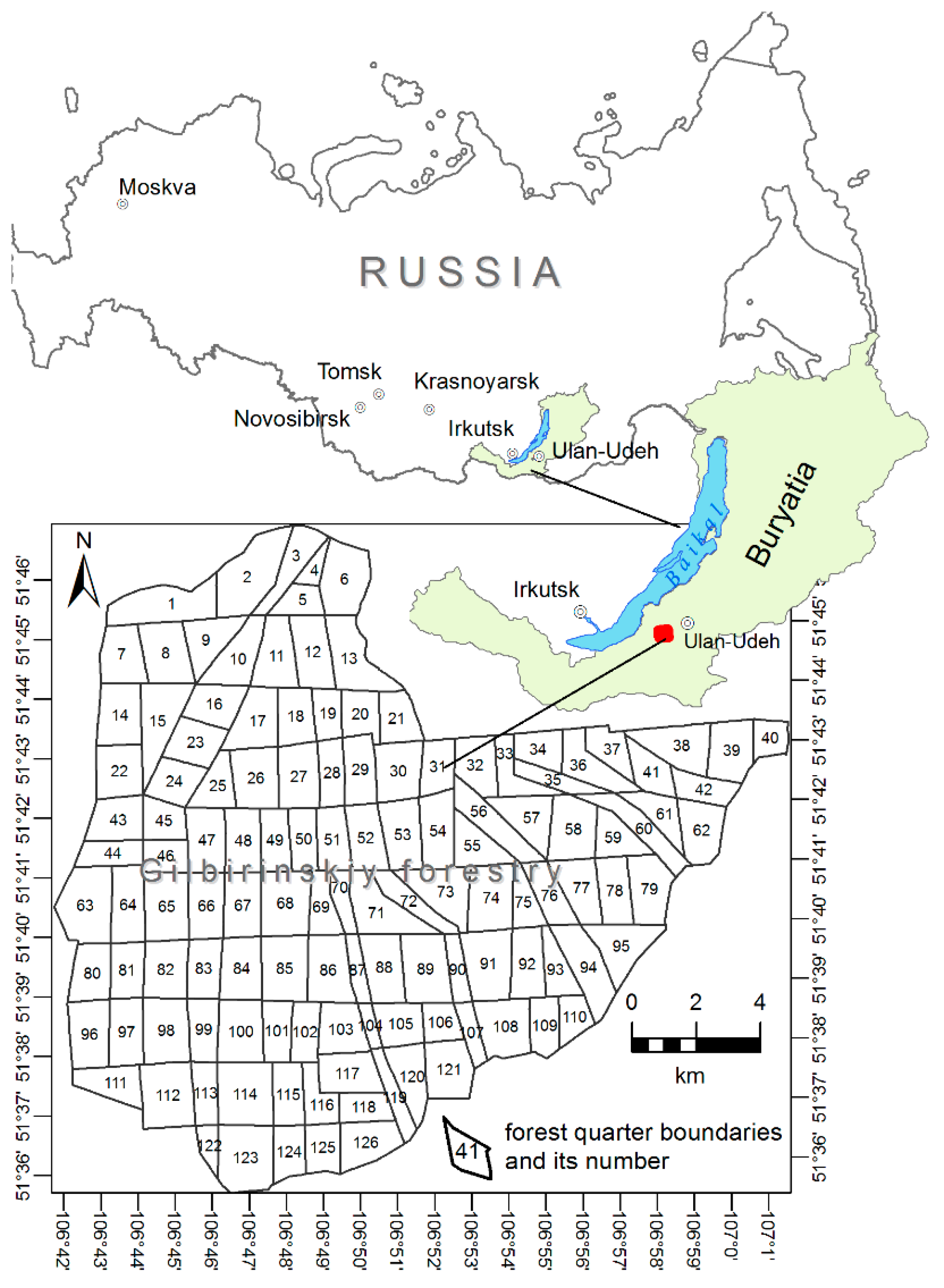
Figure 2.
Image of grass elements: stem (top) and leaf blades (bottom).

Figure 3.
Geometry of the solution area.

Figure 4.
Geometry of the solution area.

© 2019 by the authors. Licensee MDPI, Basel, Switzerland. This article is an open access article distributed under the terms and conditions of the Creative Commons Attribution (CC BY) license (http://creativecommons.org/licenses/by/4.0/).
Share and Cite
MDPI and ACS Style
Baranovskiy, N.; Demikhova, A. Mathematical Modeling of Heat Transfer in an Element of Combustible Plant Material When Exposed to Radiation from a Forest Fire. Safety 2019, 5, 56. https://0-doi-org.brum.beds.ac.uk/10.3390/safety5030056
AMA Style
Baranovskiy N, Demikhova A. Mathematical Modeling of Heat Transfer in an Element of Combustible Plant Material When Exposed to Radiation from a Forest Fire. Safety. 2019; 5(3):56. https://0-doi-org.brum.beds.ac.uk/10.3390/safety5030056
Chicago/Turabian StyleBaranovskiy, Nikolay, and Alena Demikhova. 2019. "Mathematical Modeling of Heat Transfer in an Element of Combustible Plant Material When Exposed to Radiation from a Forest Fire" Safety 5, no. 3: 56. https://0-doi-org.brum.beds.ac.uk/10.3390/safety5030056
Note that from the first issue of 2016, this journal uses article numbers instead of page numbers. See further details here.