How Cognitive Biases Influence the Data Verification of Safety Indicators: A Case Study in Rail


1
Safety and Security Science Group, Delft University of Technology, Jaffalaan 5, 2628 BX Delft, The Netherlands
2
Cognitive Psychology Unit, Leiden University, Wassenaarseweg 52, 2333 AK Leiden, The Netherlands
3
TNO Leiden, Schipholweg 77-89, 2316 ZL Leiden, The Netherlands
*
Author to whom correspondence should be addressed.
Safety 2019, 5(4), 69; https://0-doi-org.brum.beds.ac.uk/10.3390/safety5040069
Submission received: 20 July 2019
/
Revised: 28 September 2019
/
Accepted: 11 October 2019
/
Published: 15 October 2019
(This article belongs to the Collection Occupational Health and Safety in A Changing World: Realities, Challenges and Perspectives)
Abstract
:The field of safety and incident prevention is becoming more and more data based. Data can help support decision making for a more productive and safer work environment, but only if the data can be, is and should be trusted. Especially with the advance of more data collection of varying quality, checking and judging the data is an increasingly complex task. Within such tasks, cognitive biases are likely to occur, causing analysists to overestimate the quality of the data and safety experts to base their decisions on data of insufficient quality. Cognitive biases describe generic error tendencies of persons, that arise because people tend to automatically rely on their fast information processing and decision making, rather than their slow, more effortful system. This article describes five biases that were identified in the verification of a safety indicator related to train driving. Suggestions are also given on how to formalize the verification process. If decision makers want correct conclusions, safety experts need good quality data. To make sure insufficient quality data is not used for decision making, a solid verification process needs to be put in place that matches the strengths and limits of human cognition.
1. Introduction
The field of safety and incident prevention is becoming more and more data based. Organizations and institutions gather and analyze more data than ever before. Representatives from many different professional domains seek the benefits of the technological developments. Most are already implementing (big) data methods ranging from the traditional statistical analysis to state-of-the-art artificial intelligence and deep learning. Within the field of safety, new safety indicators can be used to find more detailed incident causes and effective solutions.
The field of safety however tends to have a constraint that is not shared by all fields: The data quality needs to be high. Decisions that are made can literally mean the difference between life and death. When the stakes are high, certainty is a well sought-after commodity, sometimes leading to overconservative choices. Data can help support decision making to create a better bridge between safety and innovation. This can be done by finding the common ground of overall improved execution of the core business, but only if the data can be, is and should be trusted.
Many examples unfortunately show that good data quality is not a given. Problems of faulty input data or algorithms can go undetected even when they occur frequently, like the following two bugs in software programs: “A programmatic scan of leading genomics journals reveals that approximately one-fifth of papers with supplementary Excel gene lists contain erroneous gene name conversions” [1] and “we found that the most common software packages for fMRI analysis (SPM, FSL, AFNI) can result in false-positive rates of up to 70%” [2].
There are multiple estimates available of the number of software bugs per number of lines of codes. Whilst the exact ratio estimates vary, it is generally accepted that there is such a ratio and when the number of lines of code increases, so do the number of bugs [3]. Some of these bugs might not affect the outcome significantly, while other software bugs can have large consequences, like the infamous and expensive bug in the software of the Ariana 5 rocket leading to a disintegration of the rocket 40 s after launch [4].
Besides software problems, unreliable information or input can also lead to the publication of incorrect results. Medical investigators have later learned that the cells they studied were from a different organ than expected. Such basic specification problems are not solved by having larger sample sizes [5]. Out-of-date documents can be a cause of errors, for example if a stop sign is moved but the documents are not updated to include the new location. Errors can also occur at a later stage, for example during data integration. Data integration has become more difficult due to a larger range of different data sources containing different data types and complex data structures [6].
The impact of low data quality can be very high, depending on the use case. If emergency services are sent to an incorrect location, the consequences can be negative and immediate. If incorrect data is used as a basis for performance indicators, the effects might not be immediately visible but can still be negative. When the indicators are used for safety related decision making, unsafe situations might appear safer than they are. On the other hand, safe situations can appear problematic, leading to unnecessary or even counterproductive measures. Especially in the era of Big Data, there is increased potential to draw erroneous conclusions based on little other than volume of data [7].
1.1. Verification Is Complicated
The above examples show the value of successful verification. Checking and judging data is however a complex task. Quality is a multi-dimensional concept including, amongst others, accuracy (both noise and errors), consistency and completeness [6]. At the moment, more data of varying quality is being collected and used than before [8]. Additionally, data consumers used to be (directly or indirectly) the data producers in many cases, whilst currently the data consumers are not necessarily also the data producers. This is because of the large range in different data sources that are used. The large data volume is also a challenge, both in amount of data per variable and in the high number of variables that can be integrated. When variables are being computed based on multiple sources, then verifying the quality of the individual sources is not sufficient. Verifying the computed variables alone is also not sufficient as problems can become less visible after sources are combined. Overall, verification can be a complex task for many reasons. Section 2.2 gives an overview of verification activities performed within the rail case study.
1.2. Cognitive Biases as Problem
In this article it is hypothesized that successful verification of data is hampered by the occurrence of cognitive biases. Cognitive biases are systematic errors in judgment [9]. This type of bias causes people to err in the same direction in the same information judgment task. The existence of cognitive biases during complex judgment tasks has been confirmed multiple times within numerous different experiments [10]. Cognitive biases have also been identified specifically within the domain of risk management, namely in incident investigation reports [11] and during process hazard analysis studies [12].
A lot of research has been done into cognitive biases since the pioneering work by Kahneman and Tversky in the early 1790′s [13,14,15]. Early research often consisted of experiments in which college students were presented with contrived questions they had to answer. As a result, it has been hypothesized that cognitive biases are an experimental artefact [16]. Research has however continued in more realistic settings and within a vast amount of topics (e.g., [17]). There is for example research on cognitive biases in specific health-compromised groups (e.g., persons with depression), different types of decision making (e.g., medical diagnosing), the negotiation process, project management and the military.
1.2.1. Preventing Cognitive Biases
Research on cognitive biases in specific domains can be very useful, because it is not easy to apply generic knowledge about cognitive biases to prevent errors. First of all, it is not efficient to try to eradicate all cognitive biases in human cognition. This is because the “slow” information processing which counteracts cognitive biases can come at a substantial cost. Our brains for instance consume 20% of our oxygen at rest and even greater proportions of our glucose, despite taking up only 2% of our body weight [18,19]. Trimmer [14] hypothesizes from an evolutionary perspective that cognitive biases arose for two reasons: (1) To reach optimal decision making in favor of evolution, and; (2) to reach a balance between decision quality and internal cost. Kahneman’s explanation [10] of cognitive biases in terms of two systems for cognition highlights the subjective experience of effortlessness belonging to the system responsible for cognitive biases. The subjective experience of the other system is one of significant effort.
Secondly, cognitive biases cannot be prevented by simply telling people about their existence. People tend to think they are less susceptible to biases than other people, which is called the bias blind spot. Pronin and colleagues [20] found that the bias blind spot was still present even after the participants read a description of how they themselves could have been affected by a specific bias. This bias blind spot is specifically related to recognizing our own biases, while people tend to recognize and even overestimate the influence of bias in other people’s judgment [21]. Whilst extensive training in recognizing one’s own cognitive biases is possible, the effectiveness is unclear and it could be very expensive.
Another option is to redesign the person-task system to inhibit the bias that interferes with the task (Fischoff, 1982 as in [15]). Planning poker is for example an estimation technique which has been specifically designed to prevent anchoring bias. Participants independently estimate for example ‘required time’ or ‘cost’ for a task and then simultaneously reveal their estimates. In this way, there is no anchor to be influenced by as there would have been if a number was spoken out loud by one person before others had made their estimates [22].
In the previous example, the problem of incorrect estimations in project planning was traced to being (in part) caused by a cognitive bias and debiasing action was undertaken. It is of course not always known which problematic errors are present within an organization or department. Errors might not be reported or recorded and especially in the case of errors as a result of cognitive biases, they might not even be noticed. Cognitive bias theory can be used to predict which errors might occur in specific tasks and thus help identify errors that are likely to reoccur. Both knowledge of cognitive biases and the specific tasks can then be used to redesign the person-task system.
Research on cognitive biases in specific domains can thus be very useful, but a search in the web of science database yielded few articles about both cognitive biases (or human factors) and big data. On the other hand, there has been some research on cognitive biases in software engineering (SE). While this field is obviously not the same as big data, it does contain some tasks with parallels to the verification process, specifically the testing of the code. The review by Mohanani and colleagues [15] provides interesting insights: The earliest paper of cognitive biases in software engineering was published in 1990, followed by one or two papers per year until an increase in publications as of 2001. Mohanani and colleagues found that most studies employed laboratory experiments, and concluded that qualitative research approaches like case studies were underrepresented. Most studies focus on the knowledge area SE management, whilst many critical knowledge areas including requirements, design, testing and quality are underrepresented.
The next sections of this article describe the method used in this study and the identified biases. The remainder of this introduction will first be used to explain what cognitive biases are and what the generic mechanism is behind this specific type of errors. Knowledge of this mechanism helps to understand the chosen methodology and the five cognitive biases that will be discussed in the results section.
1.2.2. Cognitive Biases: System 1 and System 2
Burggraaf and Groeneweg [11] (pp. 3–4) clarify the mechanism behind cognitive biases as follows: “According to the dual-system view on human cognition, everyone has a system 1 (fast system) and a system 2 (slow system), also known as the hare and turtle systems. Our system 1 generates impressions and intuitive judgments via automatic processes while our system 2 uses controlled processes with effortful thought [9]. System 1 is generally operating, helping you get around and about quickly and without effortful thought. Questions like “1 + 1 = …?” or “The color of grass is...?” can be answered without a lot of effort. The answers seem to pop up. When our system 1 does not know the answer, our system 2 can kick in [10]. System 2 requires time and energy, but can be used to answer questions like “389 times 356 = …?” The switch between system 1 and system 2 based on necessity, is an efficient approach. The problem is however that system 1 often provides an answer, even though the situation is actually too complex. We often think the answer from system 1 is correct, because it is difficult to recognize the need for system 2 thinking when system 1 answers effortlessly, but this is actually when a cognitive bias can occur. The main problem leading to cognitive biases is therefore not that people cannot think of the right solution or judgment (with system 2) but that people do not recognize the need to think effortful about the right solution. This lack of recognition also explains why making cognitive biases is unrelated to intellectual ability [23].
1.2.3. System 1: Automatic Activation
One of the mechanisms underpinning system 1 is the automatic spreading of activation that occurs within the neural networks of our brain. The spreading activation theory postulates that whenever a concept is activated, for example after seeing it or talking about it, this activation automatically spreads out towards the other information that the particular concept is related to [24]. This automatic spreading of activation can lead to cognitive biases when irrelevant information is activated and/or insufficient relevant information is activated [9]. This follows the description of judgement biases “as an overweighting of some aspects of the information and underweighting or neglect of others” ([9], p. 1).
Information or knowledge is not stored randomly in the brain but in meaningful networks, with related concepts close to each other. The information that is more closely related to the concept becomes activated more strongly than the information that is less closely related to the concept. When information is activated in the brain, the chance of thinking about it is increased [24]. We can for example activate the concept of the animal sheep in your brain by talking about sheep and how they walk around, eat grass and bleat. If we would now ask you: “Name materials from which clothing can be made,” we can predict that you will think of wool first, before thinking of other materials, because it was already slightly activated along the concept of sheep. Some other materials might come into your mind via system 1 quite quickly as well, while you will have to search effortful with system 2 to think of final additional options.
The mechanism of automatic activation in the context of cognitive biases is clarified further below by taking the confirmation bias as an example. The confirmation bias describes the process in which people search for, solicit, interpret and remember information that confirms their hypotheses and discount or ignore information that disconfirms them. It is caused by information processes that take place more or less unintentionally, rather than by deceptive strategies [25,26]. When testing a hypothesis, the activation of the hypothesis increases the accessibility of information in memory that is consistent with the hypothesis [27]. For example, when one considers the folk wisdom that opposites attract, multiple examples of couples of two different people are automatically activated, and the person judges the folk wisdom as true indeed. Or multiple examples are activated of how you and your partner are different and yet so good together. However, when one considers the folk wisdom that birds of a feather flock together, multiple examples of couples of two similar people (perhaps even the same couples as before, but now with respect to different parts of their personality) are automatically activated, and the person judges the folk wisdom as true indeed. Counterevidence for each piece of folk wisdom is not automatically activated, because it is not close to the activated concept in the network of activation. To activate counterevidence, one must actively think of counterevidence and thus use his or her system 2.
The enhanced activation of confirming information also influences the perception of other confirming information, which is then easier to process and activate. One can for example read an article with two consistent pieces of information and two inconsistent pieces of information and yet feel that the author’s hypothesis is supported as the consistent information is processed and remembered more easily, without the need for effortful thought [28]. A countermeasure is to think of alternative scenarios, alternative hypotheses and a good old-fashioned dose of effortful thought. Multiple experiments on biases have shown that the instruction to retrieve incompatible evidence did indeed alter judgment, while instruction to provide supporting evidence which was already automatically activated, did not alter judgment [9].
1.2.4. Relation between System 1 and System 2
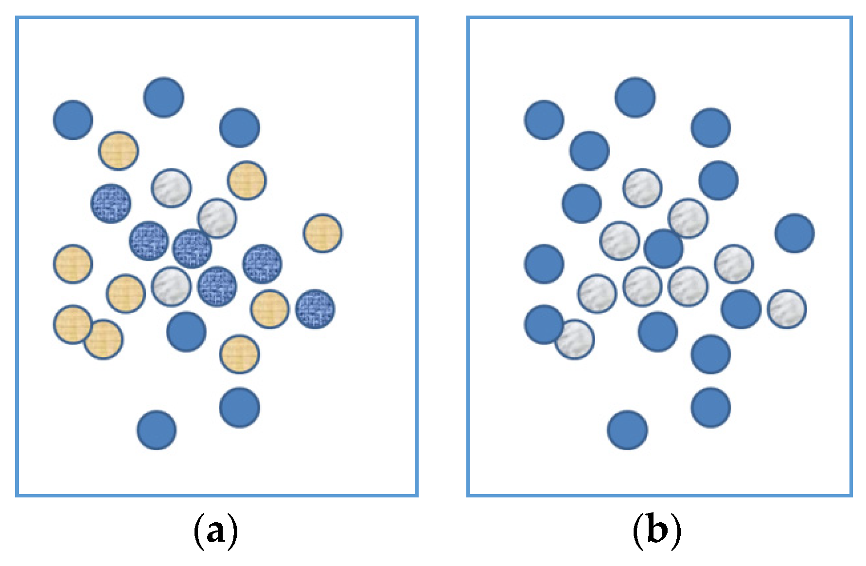
For explanation purposes, the terms ‘system 1′ and ‘system 2′ were used. It is important to note, that in this article, they are not considered as separate independently operating systems. The automatic spreading of activation as part of system 1 is a core functioning of the brain and shall always occur. It might not always be sufficient to lead to a direct answer, but the mechanism is present. Preventing cognitive biases is therefore not a matter of trying to switch off system 1 thinking, but of adding system 2 thinking, which means activating other relevant knowledge apart from the automatically activated concepts. It is not possible to suppress the automatically generated activation. The two images below are meant to illustrate this. Both images (see Figure 1) contain the capital letter A. When seeing only Figure 1a, it tends to be hard to see this letter. More noticeable are other patterns like the clustering of yellow on the bottom left and the wrinkly line through the middle. In Figure 1b, containing the exact same ordering of the circles, it is very easy to see the letter A. When people know the ‘correct answer’ after viewing Figure 1b, they are able to see the letter A in 1a, but still find it quite hard to suppress the other patterns. These other patterns tend to ‘compete’ while one tries to see the letter A. It is very hard to ignore the irrelevant information, even when you know it is irrelevant.
This is one of the key elements in identifying cognitive biases. The first cue is that they are errors which we tend to make over and over again. However, when we are capable of giving the correct answer, it is not because we are able to prevent the thought that feels intuitive, from occurring, but are able to correct it with a more reasoned thought. It is this pattern of being tempted to give an incorrect answer, which is characteristic to these types of errors.
So far, we have talked about generic cognitive biases which occur across domains. The mechanism behind these biases can also lead to more specific errors. These more specific errors are the result of the general mechanism in combination with specific knowledge about a domain, or domain-specific associations. The domain-specific manifestations of the biases will be called ‘cognitive pitfalls’ from this point on. The hypothesis is that there are cognitive pitfalls present in the verification process. The accompanying question is: which cognitive pitfalls can occur during the verification of data (for a quantitative safety indicator)?
2. Materials and Methods
Mohanani and colleagues [15] state in their review on cognitive biases in software engineering that qualitative research approaches like case studies are underrepresented, with most empirical studies taking place in laboratory settings. For the current research, the case study method was used. Yin [29] wrote in his book on case study research: “In general, case studies are the preferred strategy when ‘how’ or ‘why’ questions are being posed, when the investigator has little control over events, and when the focus is on a contemporary phenomenon within some real-life context.” (p. 1) He goes on to say that “the case study allows an investigation to retain the holistic and meaningful characteristics of real-life events—such as individual life cycles, organizational and managerial processes, neighborhood change, international relations, and the maturation of industries.” (p. 3) The case study method makes it possible to cover the contextual conditions, which are essential for the current study [29]. One of the seminal ideas that emerged from case studies includes the theory of groupthink from Janis’ case on high-level decision making [30].
In the current study, participation-observation and informal interviews were used to collect information and identify errors during the verification of a safety indicator. The identification of cognitive pitfalls was guided by theoretical propositions, specifically a number of criteria.
2.1. Method of Pitfall Identification
The method of identifying cognitive pitfalls consisted of (1) identifying errors, (2) checking whether the errors were possibly caused by system 1 thinking and (3) identifying the common ground between errors independent of the specific context, but within the verification process and (4) explaining the error in terms of system 1 automatic activation.
- 1.
- Identifying errors
The word ‘error’ here refers to having held an incorrect belief. In order for an error to be recognized, one must realize and believe that his previous statement was not true. In other words, an error has occurred when a person retracts their statement saying they no longer believe it is true.
- 2.
- Check whether the errors were possibly caused by system 1 thinking without system 2 compensation
Three cues were used to check whether the error could have been caused by system 1 thinking. A or B should occur and C.
- Tendency to have the exact same incorrect belief again by the same person, despite having been aware of its incorrectness.
This cue corresponds to the hard-wired nature of system 1 thinking and reduces the chance of the specific error manifestation being the result of randomness. For example, when there is a different error inducing factor, like time pressure, this can cause errors in a wide range of tasks and the resulting error, error A, could just as easily have occurred as error B. When error A only occurs once, this is not necessarily a reoccurring error that we as humans are vulnerable to due system 1 thinking.
- b.
- Other people have the same incorrect belief (or had it cross their mind before correcting themselves).
This cue corresponds to the characteristic of cognitive biases being person independent, and, like cue A, reduces the chance of the specific error manifestation being the result of randomness.
- c.
- The person had/could have had access to the correct information via system 2 thinking.
A false belief is not caused by system 1 thinking if the person simply did not have access to the correct information. For example, if a person was told that it takes three hours for a certain type of tank to fill up and he or she believes this until finding out it actually takes four hours, this person had an incorrect belief, but not because of system 1 thinking/a cognitive pitfall. However, consider the following scenario: there are two trains approaching a signal showing a red aspect, and both trains have the same required deceleration to still be able to stop in front of the red signal, but train A is closer to the red aspect than train B. Given that all other factors are equal, which train is at the highest risk? In this scenario someone might now answer ‘train A, because it is closer’, but after discussion say: ‘In my first answer I did not consider that train B must have a higher speed than train A, therefore I don’t think it is train A anymore, but train B’. The rejected belief in this example can be the result of system 1 thinking, because the person did not hear any new information, only used already known information in answering the question, which he or she had not done before. False assumptions are also a candidate for system 1 thinking. For example, one might assume that a sensor is gathering the correct data. If it later turns out that the gathered data was incorrect, then the previous incorrect assumption could have been a system 1 error. The argument ‘but we did not know the sensor was faulty’, does not change the fact that the persons in theory did have access to the correct information. By thinking about the quality of the sensor, they could have realized that the quality was in fact unknown and could be bad. This is in contrast to for example being asked what the capital is of a country. If you have never heard or read what the capital of the country is, no amount of thinking will lead to the correct information.
- 3.
- Identifying cognitive pitfalls
When the same type of error manifestation occurs within different topics, for example with respect to different data sources, then the common cognitive pitfall is identified.
- 4.
- Explaining pitfall in terms of system 1 automatic activation
As a final step, it should be possible to explain the occurrence of the pitfall in terms of system 1 automatic activation. The explanations listed in the results section sometimes include schematic representations of knowledge structures and the automatic activation. These visualizations are not empirically proven within this study, but included to illustrate how the theory of automatic activation can explain the occurrence of the cognitive biases. Even though it is not yet clear how exactly information is stored in our brains, being able to explain errors in terms of system 1 thinking and the automatic spreading of information is an indication that interventions tailored specifically to cognitive biases could have more effect than other error prevention approaches.
2.2. The Case Study: Deceleration to SPAD
Within the rail domain, one of the key dangerous events is a train running through a red light, also called a SPAD: Signal Passed at Danger. ProRail, the Dutch rail infrastructure manager, has developed a proactive safety indicator called ‘Deceleration-to-SPAD’ (DtSPAD) in cooperation with NS Dutch Railways (NS). This indicator can be calculated for any train approaching a red light and indicates the deceleration that the train needs in order to still be able to stop in front of the red light. A DtSPAD that is higher than the total available braking power of the train means that the train will pass the signal at danger unless the signal clears before the train reaches it. Besides DtSPADs higher than 100% of available braking power, high DtSPADs can also be interesting for safety monitoring as they indicate small buffers. The maximum DtSPAD can be taken to illustrate the smallest buffer the train driver had per red aspect approach. The distribution of maximum DtSPADs can then be used to monitor train driver behavior and effects of interventions on behavior.
The basic formula to calculate Deceleration-to-SPAD is a half times the current speed of the train squared, divided by the distance to the red signal. The location and speed of the train are recorded by Global Positioning System (GPS) sensors which are present on the trains. A Deceleration-to-SPAD value is calculated for every entry of speed and location supplied by the GPS sensor while the train is approaching a signal showing a red aspect. The DtSPAD calculation starts after a train has passed a signal showing a yellow aspect that is caused by a red aspect. The calculation stops when the train is no longer approaching a signal showing a yellow or red aspect [i.e., when he receives new movement authority].
Variables that were used to calculate DtSPAD include:
- distance from GPS sensor to head of the train (inferred via the driving direction of the cabin with the sensor and train-type dependent possible sensor positions);
- location of the signal in longitude and latitude;
- signal aspect at given times;
- longitude and latitude of GPS sensor;
- speed of the train;
- for combining data: Train number, train type and time;
- originally needed for time calibration because of non-synchronous clocks: Time the train passed a signal according to hardware in the tracks and according to GPS sensor.
The data was gathered from existing systems from ProRail and NS, pertaining to the whole of the Netherlands. None of these systems were specifically designed or chosen with the goal in mind of calculating the DtSPAD indicator. The used GPS sensors were for example installed by the organization performing the maintenance of the trains with the aim to find the location of the trains due for maintenance. There are other sources monitoring train location, but the data from these sensors was chosen because of the higher logging frequency compared to other systems providing data at the time.
One of the use cases for the DtSPAD was to identify factors that correlate with higher or lower DtSPAD levels. Potentially correlating factors were therefore also verified apart from the DtSPAD variable and the variables used for its computation. Both qualitative and quantitative verification methods were used as recommended by Cai and Zhu [6]. Where possible, quantitative variables were compared to a reference value. For example, the distance traveled between two points according to the GPS data was compared with the distance traveled according to the time between the two points and the speed. Variables were also checked for impossible or improbable values (e.g., higher speed or deceleration than the trains are capable of) or impossible combinations (e.g., low risk value, but negative distance to red signal). Problematic values were not simply removed, but rather the individual cases were examined to identify the cause, as part of the qualitative approach, and fix the cause. Patterns were also examined for oddities (e.g., when 99% of the values follow a curve and some do not) and the deviating approaches investigated. We analyzed the data in the programming language and software environment ‘R’, using our own code. The data that was used for verification covered periods of one month up to a year. The exact period varied due to the iterative nature of the verification process in which improvements to the data source or code could sometimes not be implemented retrospectively. As a result, data from the last update up to the day of analysis was used.
Apart from examination of the variables, qualitative verification of the code itself was also performed occasionally, as will become evident in Section 3.5.
The cognitive pitfalls framework was applied to the verification process from the start of the verification in March 2016 until October 2016.
3. Results
Five cognitive pitfalls were identified during the verification process: ‘the good form as evidence’-error, the ‘improved-thus-correct’ fallacy, ‘Situation-dependent-identity-oversight’, ‘Impact underestimation’ and ‘beaten path disadvantage’. These pitfalls will be clarified by an example, explanation of the pitfall and examples from the case study, after which the implication of the pitfall is discussed. It is noted that this list of five is not necessarily exhaustive. It is possible that there are other cognitive pitfalls relevant for a given verification process that are not in this list because they did not occur during this specific case study or did not lead to salient errors.
3.1. Pitfall 1
3.1.1. Example
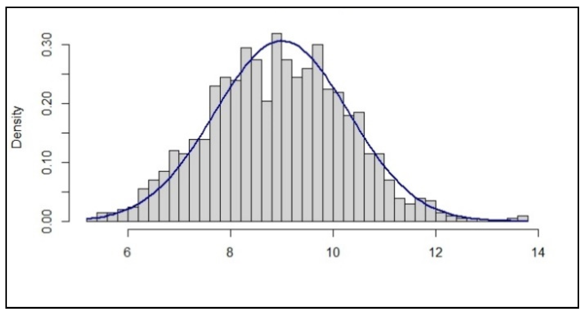
In this example we are looking at a variable which we expect, based on theory, to follow a normal distribution. We check the actual distribution of the real data as a means to check the quality of the data. The image below, Figure 2, is the result. What conclusion do we draw with respect to the quality of the data?
A typical response would be that the data is approximately normally distributed. The data looks ‘about right; quite good’, etcetera. Generally, this is seen as a reassurance that the data is correct and we can proceed.
3.1.2. ‘The Good Form as Evidence’-Error
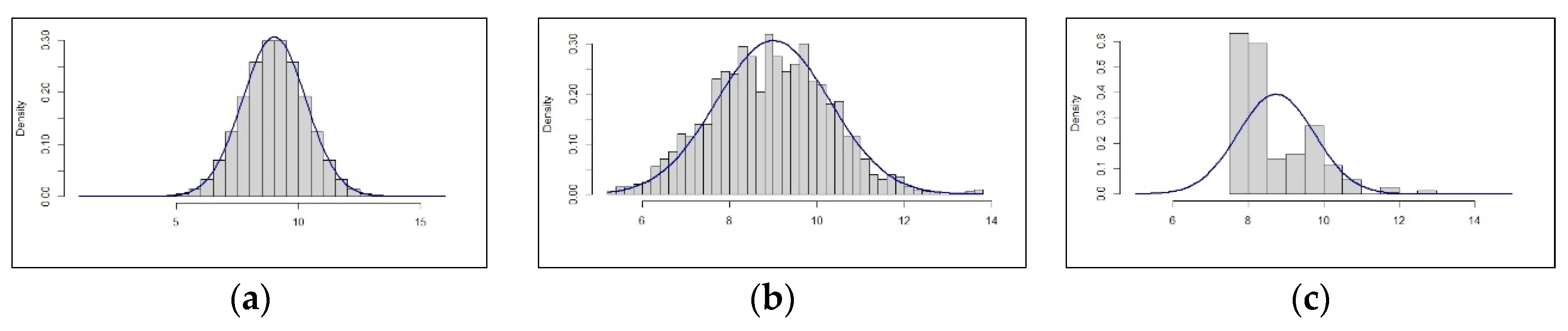
The images in Figure 3 roughly show all three situations which can occur when visualizing the data: (A) the data follows the distribution perfectly, (B) the data distribution looks about right and (C) the data looks awful in the sense that it does not meet expectations at all.
In the first case, the conclusion typically is: “That is too good to be true. This is proof that something is not right. We need to check this.” As mentioned before, the conclusion in the second case typically is: “Approximately fits the distribution. This is proof that the data is correct.” As well, in the third case: “This does not look at all like expected. This is proof that something is probably not right. We need to check this.” Whilst the first and third conclusion are correct and lead to the desired behavior of further verification, the second conclusion is not correct. This type of visual representation is not proof that the data is correct, since this distribution can occur as the result of correct, but also as the result of incorrect data. We tend to underestimate the chance that the underlying data is incorrect when we see this kind of ‘good form’ visualization. Incorrect data here refers to either faulty data sources or erroneous algorithms. The actual chance of the data being incorrect when we consider the evidence of ‘good form’ can be calculated via Bayes’ theorem:
The actual chance includes (1) base rates of incorrect data and of good form and (2) the estimated chance of incorrect data leading to good form. In chance estimates like these, people tend to rely on representativeness and not include the base rate. This fallacy is called the base rate neglect, previously described by Tversky and Kahneman [13] as “insensitivity to prior probability of outcomes”. This is possibly part of why we underestimate the presence of incorrect data in the face of ‘good form’. Another part of the reason can be our association between appearance and quality. We have a deep-rooted association between ‘bad’ and ‘ugly’ or ‘too perfect’. Villains tend to be depicted as physically ugly persona’s or too perfect persona’s, usually con artists. The strength of this association is underscored by the surprise we feel when confronted with something that does not fit this association. In the DtSPAD project, we looked at a distribution of the DtSPAD variable which resembled the ‘good form’ as previously displayed. Even after knowing that the displayed data was incorrect (because an error in the code was identified), we were still inclined to draw conclusions based on the data we saw. The notion that bad data could look like good data remained counterintuitive, while the intuitive association automatically gets activated: ‘but it is good looking data, so good quality data.’
In reality, it is possible that bad data looks good. Even though we do not know the numbers to the base rates or relations, we can enter hypothetical data in Bayes’ theorem to get a feel for the actual probability of incorrect data when visual inspection shows ‘good form’.
In the first draft of an indicator, let’s assume that the base rate of incorrect data is high, say 0.7. When incorrect data leads to good form with a chance of 0.3 and correct data leads to good form with a chance of 0.95, the probability is:
=0.3 × 0.7/(0.3 × 0.7 + 0.95 × (1 − 0.7)) = 0.21/0.495 = 0.42
This example indicates that it is actually highly likely that data is incorrect, even though it looks good.
Even when we assume that incorrect data only leads to good form in 10% of the cases, the chance of the data being incorrect in the face of ‘good form’ is still relatively high (0.20).
3.1.3. Implication
Visual inspection of the data, for example by looking at the distribution, is an essential part of the verification process. It can be an efficient way to verify problems after detecting for example outliers or a deviation in distribution. However, once the data has improved in such a way that its form no longer shows any worrisome elements, this should not be used as proof that the data is now correct. At this point in the process, other methods are needed to proof that the data quality is good (enough). One method is to compare a variable with another variable which is supposed to measure the same thing. In our verification project we for example compared time passed according to the time stamp with time passed according to distance travelled divided by the speed. This lead to the discovery that the time stamp was not accurate even though the DtSPAD data looked good upon form inspection. In our case, the time stamp in the dataset was not the actual time logged by the GPS sensor but the time that the logging took place of the GPS signal once it arrived at a server where the time of the server was taken. Due to differing latency times this lead to cases in which the timestamp indicated that two seconds had passed while in fact, given the distance travelled and the speed, zero to seven seconds had passed. This varying time deviation was very problematic for our indicator because it can lead to relevant data points not being included (still approaching a red light but data no longer included).
While the use of a different timestamp than the GPS time might seem strange, it was actually very straightforward for the persons who had set up the system. The alternative time was what they called “the train time” and made it easy to combine different measurements because they all had the same “train time” and the time latency was not a significant issue for their usage. It just never occurred to them that it might be a problem for the DtSPAD project, just as it did not occur to us before verification that there could be another “time” than the actual (GPS) time.
To further improve verification, Van Gelder and Vrijling [31] highlighted the importance of extending visual inspections and statistical homogeneity tests with physical-based homogeneity tests. By considering whether the data can be split in subsets based on physical characteristics of the individual data points, it can be prevented that the variable as a whole seems homogeneous, while it is in fact a combination of two or more different distributions that could, by chance, look like one homogeneous distribution when put together.
3.2. Pitfall 2
3.2.1. Example
For the DtSPAD indicator we created a categorizing variable indicating whether a yellow aspect was planned or not planned. This variable was not always correct. We discovered that sometimes a yellow aspect was characterized as ‘unplanned’ while it was in fact part of a planned arrival. It turned out that short stops of trains were not yet included as planned stops. A bug fix was done to include the short stops. What is now our view on the quality of the indicator?
3.2.2. The ‘Improved-Thus-Correct’ Fallacy
The intuitive response is to think the planned/not-planned indicator is now correct. This is called the ‘improved-thus-correct’ fallacy. In reality, the quality of the indicator is not necessarily good after improvement. The improvement can have caused new problems, especially in coding where bug fixes can create new bugs. However, even if the improvement was implemented correctly, there can still be problems within the data which are not fixed by this specific improvement. These are straightforward notions, yet we tend to forget them which leads to the ‘improved-thus-correct’ fallacy. This fallacy can present itself by someone saying an indicator is correct after it has been improved without knowing the actual quality, but more often the fallacy will result in someone not explicitly stating the quality is now good, but forgetting the need to recheck the quality.
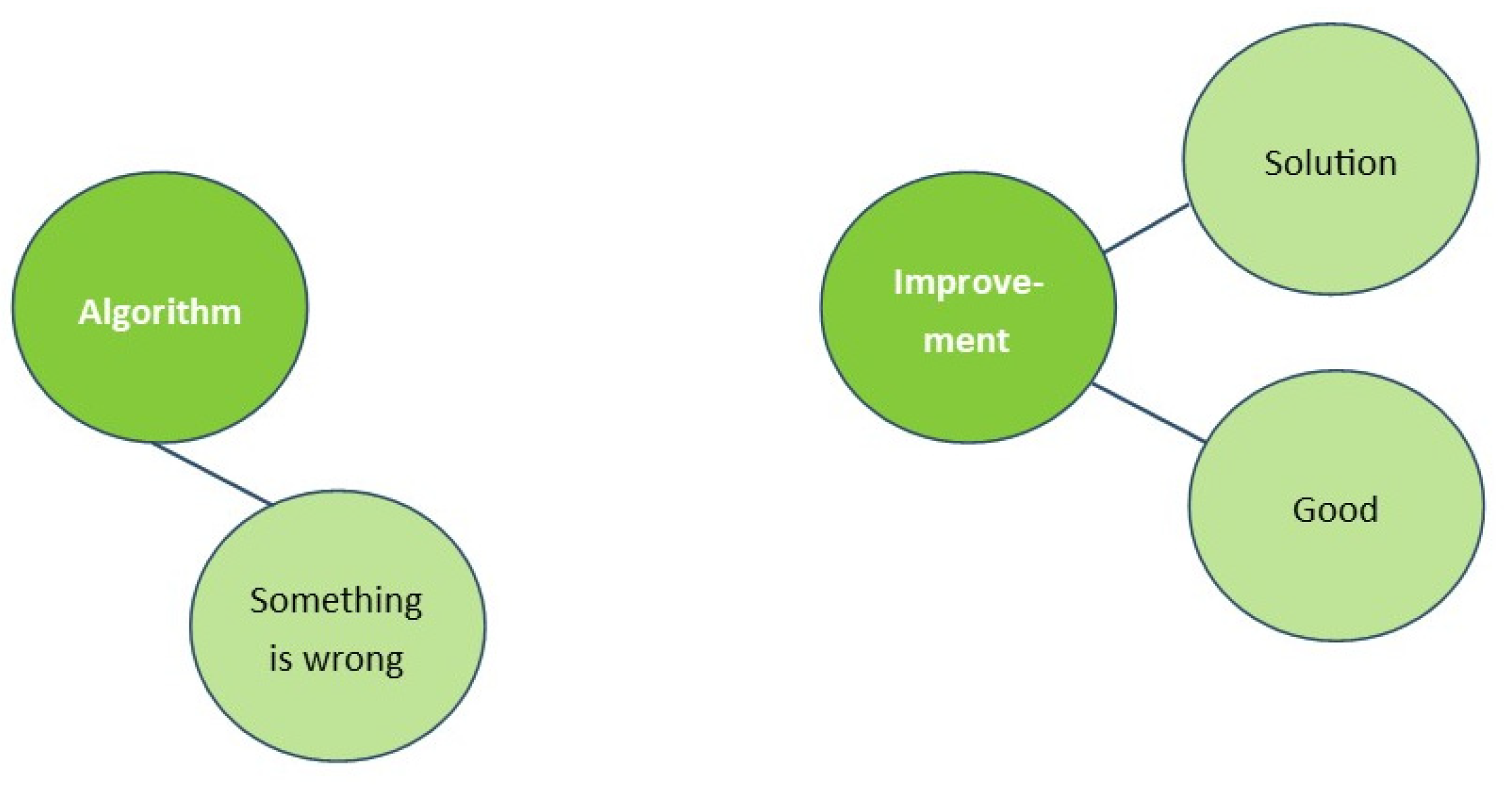
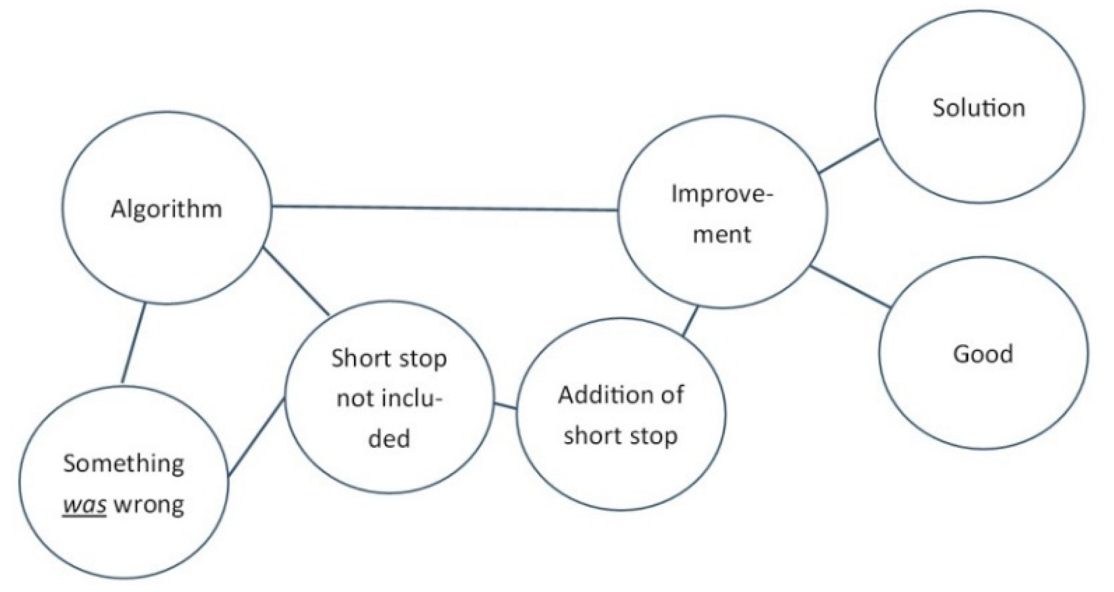
This phenomenon can be clarified by thinking of the structure of knowledge in our brain and the automatic activation of associations. Imagine the concepts ‘Algorithm’ and ‘Improvement’ being present in our brains. In the situation as stated by the example, we are aware that something is wrong with the algorithm and thus it is associated with ‘something is wrong’ and not yet with ‘improvement’. Activation of ‘algorithm’ will now also automatically activate ‘something is wrong’, while activation of ‘improvement’ activates other positive concepts like ‘good’ and ‘solution’ (See Figure 4).
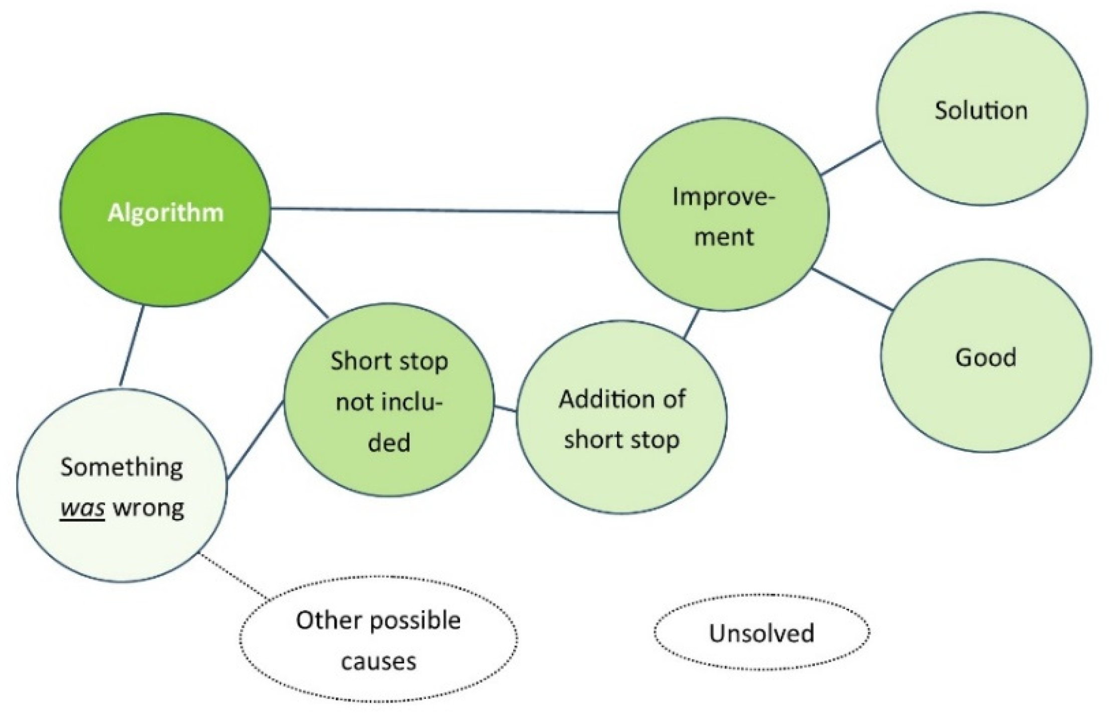
After the bug fix, the notion of ‘something is wrong’ changes to ‘something was wrong’ and ‘algorithm’ is now also associated with ‘short stop was not included’ and ‘improvement’, which both share ‘addition of short stop’ (See Figure 5).
The activation of ‘algorithm’ will now also activate ‘improvement’ and ‘good’. The aspect ‘something was wrong’ will still be activated as well, but this enhances what was wrong ‘missing short stop’ and then the solution which again is connected to ‘improvement’. At the same time, the idea that there might have been other causes as to why something was wrong with the algorithm is not automatically activated as it is not connected (See Figure 6). During the process there was no learning and thus no reason for neurons to connect between ‘something is wrong’ and any other cause which does not have a concrete representation yet, unlike for example ‘short stop was missing’ which can be vividly activated. That is to say, other possible causes ‘do not have a face’ and therefore are not automatically activated while other concepts are, providing a system 1 answer that is easy to accept.
In our verification project it was noticeable that when the generic status of the planned/unplanned indicator was questioned, the answer was: ‘there was a bug fix with a high impact two weeks ago to include short stops’. While it was then not explicitly said that the indicator was now correct, the effect of the fallacy was noticeable in the fact that we tended to forget to check the current quality of the indicator. Even though it was part of the to-do list, it needed explicit reminding, otherwise it was simply overlooked. Even when the indicator was checked, the implicit assumption was that it would now be correct, noticeable by the sense of surprise when discovering new problems. This sense of surprise also occurred for another indicator which was improved and a new check was done in the sense of ‘just a formality’, which to our surprise exposed the need for more improvement.
3.2.3. Implications
This fallacy highlights that people tend to overlook the need to check something (e.g., an algorithm) again after improvements. Therefore, it is important to create an explicit step within the verification process to perform a quality check after every improvement. Additionally, it is important to phrase the current quality not in statements of last improvements, but in a number or unit, like % unknown or % error, or even something more qualitative, like ‘checking for 5 h did not lead to the discovery of new errors’. Even if the current quality cannot yet be specified, the empty field will indicate the need to (re)do a quality check.
3.3. Pitfall 3
3.3.1. Situation-Dependent-Identity-Oversight
When thinking about the quality of an object, two problems occur. One is that it is hard for us to imagine all factors that can influence the quality. Examples include human factors issues, like things that can go wrong during installation, or the influence of human behavior on the collected results.
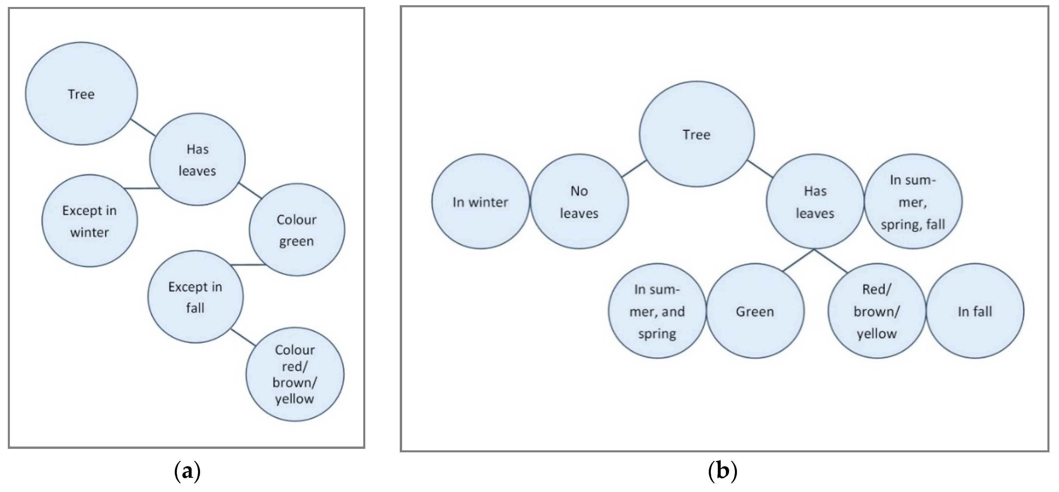
Discovering that the quality is very different than expected because of an unforeseen factor is usually followed by the phrase: ‘I did not think of that’. While this can be a serious problem, the inability to think of such factors is not a system 1 problem. In fact, it is a problem that remains, even when we use our system 2 thinking, since it is more a matter of the knowledge we have, our previous experiences and creativity. Being aware of our inability can help us to collect more information or choose different approaches, like performing verification measurements on the sensor once it has already been installed. This is however where the actual system 1 problem, the cognitive pitfall comes in: we have the tendency to overlook the fact that objects actually have differing identities or differing qualities in different situations. We do not think in terms of ‘this object = x in situation A and the same object = y in situation B’. Instead we just say ‘this object is x’. For example, when I ask you, what color do the leaves of an oak tree have? Your answer will be ‘green’. As well, anyone will accept this answer as true. Anyone will agree that indeed the leaves of an oak tree are green. We collectively accept this truth, even though all of us also know that the leaves are not always green. The fact that, even though the oak trees’ leaves are orange or yellow or brown in the fall, we still say the leaves are green, provides some inside in the way knowledge is structured in our brains. Figure 7 shown below illustrates a hypothetical structure. The concept ‘tree’ is linked to many other elements, including ‘has leaves’, which is connected to ‘except in winter’ and to ‘color green’, which is connected to ‘except in spring’ which is connected to ‘color red/yellow/orange’.
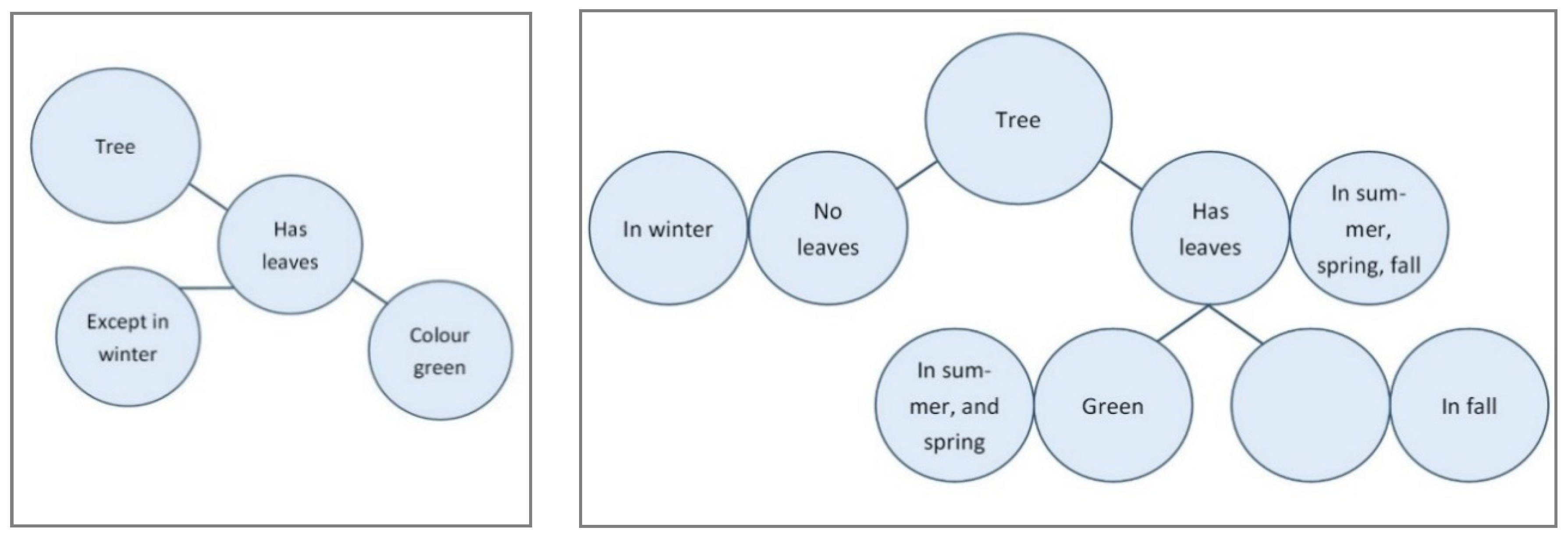
A model that incorporates a situation-dependent-identity would look more like Figure 7b above. The model on the right needs a lot more nodes to hold the same information. The structure of the model on the left makes it possible to get to a first answer quickly and efficiently (via automatic activation), with the possibility to obtain the rest of the knowledge when thinking more about it (system 2). The advantage of the model on the right however is that it is more noticeable when you do not know the answer in a specific situation, for example the color of leaves in fall, since there will be a blank node connected to that situation. In the model on the left, on the other hand, when you do not know the color of the leaves in fall, the bottom of the model will simply fall off and you can still answer the question ‘what color do leaves of trees have?’ without any empty spaces (see Figure 8).
3.3.2. Example
A hypothetical big data project uses temperature as one of the variables to calculate the final indicator. The used digital temperature sensor has been tested in the lab and logs the temperature every 30 s with an accuracy of 0.3 °C. For this project, an accuracy of ±0.5 °C or better is sufficient. Is the data quality of the sensor sufficient for this project?
The intuitive answer is yes. However, additional relevant questions are: Is the sensor installed correctly and in the correct place when used for the project? Has it been calibrated (repeatedly)? Does it work in the used context? After the sensors are installed on tracks, the impact and vibration caused by trains driving over the tracks might disturb measurements. Does the sensor have the same accuracy over the whole range of measured temperatures? Are human acts needed to turn on/off the sensor? Are there any other context factors of the actually implemented sensor that could impact its accuracy or the logging frequency?
3.3.3. Cases
During the DtSPAD project, the tendency to think in terms of one (situation independent) description was for example noticeable with respect to the GPS-sensor. We had seen plots of the GPS locations of a train and noticed that these follow the tracks. When asked about the quality of the GPS sensor, we were therefore inclined to answer: “fairly good based on initial observation”. Sometimes we forgot to include the phrase “but the quality is very bad when the train is located in a train shed or under a platform roof”. As well, we tended to forget the possibility of other factors impacting the quality as part of our check list. Even though these elements can come up when time is devoted to this specific topic and people are in system 2 thinking mode, they might be overlooked at other times, especially during (verbal) handovers to other people or in the interpretation by other people based on written handover.
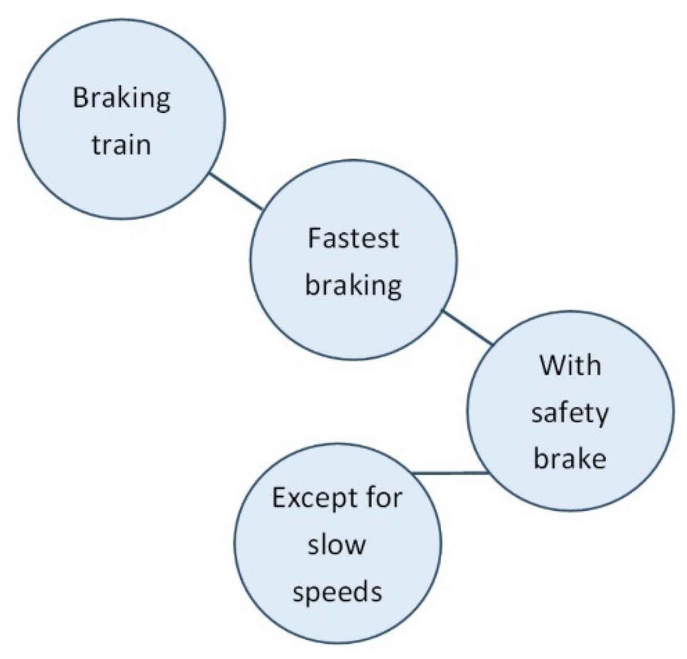
Another example of this pitfall occurred during the analysis of an error with the previous version of the indicator. This previous version looked at the remaining time available in seconds, before an emergency brake needed to be applied, instead of the required deceleration. In the dataset, we discovered trains with a negative time, indicating that they would pass a red signal, followed by a positive time, which should not have been possible. This suggested a problem in the calculation of the minimal braking distance. The minimal braking distance was calculated taking the parameters into account related to the safety brake/quick-acting brake (see Figure 9).
Repeated checks of the execution of the formula did not lead to any further insight. Eventually it was noticed that using the safety brake only leads to the shortest possible braking distance when the train is driving at a certain speed or faster. At very low speeds, the braking distance is actually shorter with the regular brake. The conceptual validity of the formula had been checked before as part of the verification but not considered as the problem. Only after other issues with respect to its execution were scrutinized and deemed well, was the conceptual validity checked again as part of the same verification and the problem found. This example again shows that thinking in terms of situation-dependent deviation is not a first intuitive approach, especially since the question (‘what is the fastest braking/minimal braking distance’) can already be answered (‘with safety brake/ this formula’) (See Figure 10).
3.3.4. Implication
To prevent oversight of factors influencing the quality, it is important to add to the quantification of the quality (accuracy and loggings frequency) for which situation this quality is applicable. For example, for the temperature sensor it could say: an accuracy of 0.3 °C when installed correctly and calibrated in a lab environment whilst measuring temperatures ranging from –10 °C to 40 °C. For other elements, it can be useful to include details about software package and expected human behavior in operation. Since it is difficult to oversee all possible factors influencing the quality it can be useful to test the quality whilst in the actual operation mode used for the project, check in a number of different ways, like with other software packages or other types of code, and to learn from other projects about which factors had an (unforeseen) effect.
3.4. Pitfall 4
3.4.1. Example
We calculate a DtSPAD value for a train on every moment a GPS location is logged. What is the influence on the DtSPAD indicator if the logging frequency would be reduced from once per two seconds to once per three seconds? Does this have a problematic impact on the quality of the DtSPAD indicator?
Based on this information, it is very hard to answer the question in detail. An exact answer does not come to mind, but system 1 immediately provides a response like ‘it is not really a problem’. We can however simply not know at this moment, regardless of our hunch that it is not very problematic. For demonstration purposes let’s consider the case of lowered logging frequency in more detail.
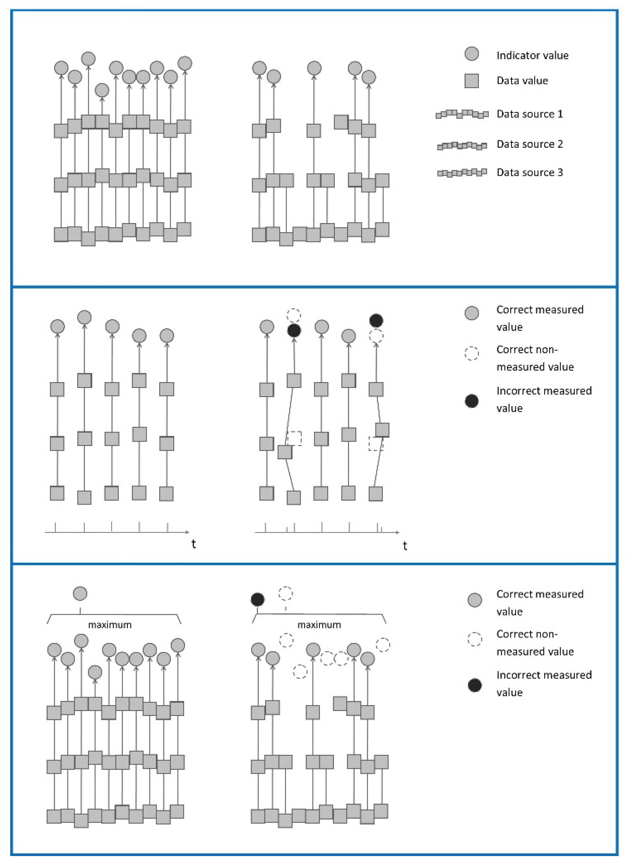
The left image (see top Figure 11) displays the ideal situation with continuous logging in which three variables are combined to create the indicator. In the situation on the right, some values are not logged leading to lower coverage in the indicator.
In the second situation (middle pane of Figure 11), there is not only lower logging frequency, but because the different variables are not logged at the same time, they need to be matched leading to lower coverage in the indicator and deviation from the actual indicator value.
In the final example (bottom pane Figure 11), the actual indicator is a selection from the data, like in our project we are interested in the maximum DtSPAD. In this case, there is deviation from the actual indicator value because a different data point is selected.
3.4.2. Impact Underestimation
The above example is meant to illustrate how complex the relation can be between one variable and the indicator and how difficult it is to oversee the impact of changes in a variable on the indicator. When we are confronted with questions like the one in the example, we actually do not know the answer, until we thoroughly analyze it. Yet, such questions do not trigger a sense of panic, because of two reasons (1) even without an exact answer we still have a rough idea that it probably does not have that much impact and (2) within humans, a sense of danger arises at the presence of signs of dangers and not by the absence of signs of safety. The former reason can be explained again by automatic activation. The small number related to the variable installs the idea of a small effect. This is a manifestation of the anchoring bias in which a specific number influences someone’s numerical estimate to an unrelated question [9,13].
3.4.3. Implication
The impact underestimation can cause small deviations in quality of a variable to, unwarrantedly, fly under the radar. When the quality of the indicator is critical, it is important to substantiate the impact of the given quality of each variable on the indicator. This requires thorough analysis and system 2 thinking whilst disregarding the system 1 feeling that there probably is not a problem.
3.5. Pitfall 5
3.5.1. The Beaten Track Disadvantage
When verifying data, texts, theories, code or formula’s, some persons prefer to take the ‘blank slate’ approach and first view the to-be-verified element and then judge. This is in contrast with first thinking of your own version of the data/text/theory/code/formula and then comparing it with the to-be-verified element. The beaten track disadvantage entails the tendency to overlook problems during verification when employing the ‘blank slate’ approach. During this approach, reading the to-be-verified element will activate the read concepts in your brain including the logic of the story and this will create a beaten track. This beaten track is easy to travel along in the sense that it is highly activated and the first ideas come up again easily. Alternative notions are activated less easily and can ‘lose’ from the beaten track.
A comparable experience we all have had is during brainstorm sessions, for example when considering a new approach or a project title or a gift for a friend. When a few suggestions have already been made, you have the tendency to think of these same suggestions again and again or the same suggestion in slightly different wording. As well, sometimes you feel you are on the brink of thinking of something new, and then another person offers their suggestion and you lose your own thought. It cannot compete with the other activation.
The beaten track disadvantage does not necessarily prevent you from noticing erroneous thinking. It mainly prevents you from including elements in your judgment that are not in the to-be-verified object, therefore causing you to overlook certain elements. You are able to judge what is done, but less able to judge what they have not done and should have done. In a verification task it is therefore useful to first consider your own version of the correct solution and then compare it with the actual solution. Even just considering all the factors to take into account and the necessary information to be collected can already be useful.
3.5.2. Example
“The possible locations to install the GPS sensor on the train differ per train. Each train has one possible location to install the GPS sensor with a set distance to the head of the train. The FTS train 4 has a distance of 54 m to the head of the train. The FTS train 6 has a distance of 86 m to the head of the train. Of all the FTS trains, only the FTS 6 trains have been equipped with a GPS sensor so far. The distance between the head of the train to the signal is calculated using Vincenty’s formula to discover the distance between longitude and latitude provided by the GPS sensor and longitude and latitude of the signal. The 86 m are then subtracted from that sensor-signal distance to get the distance between the head of the train and the signal (accepting some inaccuracies due to turns in the tracks instead of a straight line between the train and the signal).”
Above text describes part of a hypothetical calculation process. For this simplified example, a question during the verification process would be whether there are any issues with this process as described above?
When we accept the usage of Vincenty’s formula in this case, then there does not seem to be a problem with the process. Yet there is one potentially relevant question to ask: do we also receive GPS data from trains other than FTS trains? If so, then the adjustment for GPS sensor position might be incorrect. This seems like a straightforward question to ask and yet it is easily overlooked. The presence of more trains than only FTS trains with GPS data is actually a realistic situation, especially when different parts of the algorithms are written by different persons and they receive the information in fragments. The programmer who includes the distance from the sensor to the head of the train might be referred to someone knowledgeable about these distances. When this person only ever works with FTS trains he or she will only give the information related to the FTS trains and the programmer will use this knowledge in his coding.
3.5.3. Cases
One of the cases that occurred during our verification project did actually entail the adjustment for sensor distance. The distances were correctly adjusted for sensor location during the calculation of the DtSPAD. However, during an earlier version, calibration of the time was also necessary because the clocks of the sensors were not running synchronous. The calibration was done by taking the moment in time according to the GPS sensor when they passed a signal and the time according to the system in the tracks registering train passage. When we looked at the code written for this calibration, we did not register it as a problem that the actual longitude and latitude of the GPS sensor were used instead of the adjusted location of the head of the train, even though we were familiar with the issue of sensor distance even for calibration in other settings. However, when actually looking at the code, which was otherwise executed perfectly fine, the problem was not triggered. During code adjustments for the calculation of the DtSPAD with respect to the sensor distance, the programmer noted he should use this approach for the calibration as well upon which the response was: ‘did you not already do that?’, illustrating that the knowledge of its necessity was there but it was not sufficient for us to notice the glitch when looking at the code.
3.5.4. Implication
If quantitative verification with actual data is possible, this is a sound approach. When theories or algorithms need to be checked, this is however not always possible. In these types of expert-judgment verifications it is useful to discourage the ‘blank slate approach’ and encourage persons to first consider their own version of the correct solution and then compare it with the actual solution. When this is too time consuming, one can restrict the work to considering the factors to take into account when one would try to create the correct solutions themselves. These factors can then be used as a checklist or backbone to verify the element with.
3.6. Summary of All 5 Identified Pitfalls
The five identified pitfalls are summarised in Table 1 with a recommendation per pitfall.
4. Discussion
4.1. Limitations and Further Research
This ‘proof of concept’ case study of a safety indicator in the railway industry took a closer look at the human factors challenges in the verification process as part of (big) data utilization. Five cognitive pitfalls were identified to be aware of when verifying data, given the way our brains function. It is expected that knowledge of these pitfalls is relevant for other railway organizations and other industries as well, because cognitive biases in general have been proven to occur amongst all people. However, the prevalence of these pitfalls and data verification within other organizations is not known. The current study focused on testing a more extensive theoretical framework on cognitive biases in an actual setting, with a focus on providing a deeper understanding of these types of errors and their prevention. Future studies that focus on measuring the prevalence of these pitfalls would be beneficial, followed by research on the success rate of interventions.
Another limitation of the current research is that the list of five pitfalls is not necessarily exhaustive. It is possible that there are other cognitive pitfalls relevant for the verification process that are not in this list because they did not occur during this specific case study or did not lead to salient errors. Further research to identify other possible cognitive pitfalls can consist of other case studies or experimental settings with respect to data verification. This research is especially important in use cases where the results cannot be easily verified, that is when the calculated indicator does not have an equivalent indicator or predicted live data to compare it with. This is the case for safety indicators that relate to low incidence incidents, like SPADs, but can also be the case for ‘softer’ measures, like ‘safe driving behavior’ or, for example in health care, for measure like ‘improved health’ or ‘surgery success’.
Besides improving the verification process, future studies are also needed to improve other aspects of (big) data: Even when the input data is correct, the results can still be incorrect. Common errors include the sampling error causing the data to be non-representative. Even in the big data domain where the assumption often is that we have all the data, this can be a far cry from the truth if there are non-random gaps in the data [5]. Multiple comparison is also highlighted as a big data issue, meaning that the presence of a lot of variables and a lot of data will, by chance, always lead to some seemingly significant factors unless corrected for. Van Gelder and Nijs [32] also note this issue in their overview of typical statistical flaws and errors that they found upon investigation of published big data studies related to pharmacotherapy selection. Another problem is that big data solutions are notorious for focusing on correlation and ignoring causality. The Google Flu prediction algorithm for example was based on the amount of flu related google searches and was considered an exemplary use of big data, until the predictions were far off in 2013. The overestimation was likely caused, at least in part, by a media frenzy on flu in 2013 leading to a lot of flu-related searches by healthy people. Additionally, the constant improvements in Google’s search algorithm has likely had an effect on the quality of the predictions [33]. Even in cases where the prediction model can be updated based on new information of the changing circumstances, this might already have led to losses when the results were acted upon and the cost of a false-alarm or miss are high. The universal occurrence and especially recurrence of such errors (e.g., not taking changing relationships into account, multiple comparison and sampling error) can be illuminated by investigating the role that cognitive biases play in their occurrence.
4.2. Advocated Perspective and Recommendations
For each cognitive pitfall identified in this article, recommendations were given to prevent them from leading to errors. When thinking about tackling errors within risk monitoring, it is important to keep in mind that, given the way our brains function, it is expected that errors occur within information judgment tasks as part of risk monitoring. These errors occur regardless of the intelligence of the persons performing the tasks and are not person-dependent. Creating awareness among persons about these facts, the way we think and our tendency to fall into these pitfalls is part of the approach against cognitive pitfalls. Secondly, and equally if not more important, measures can be taken to improve the process itself and minimize the chances that people will make these type of errors.
This second approach consists of formalizing the verification process to create reminders of the factors that need to be considered with system 2 thinking so the errors do not occur. These formalizations of the verification process are not designed to take away some of the cognitive load or the thinking of the persons involved, but in contrast to encourage deep and reasoned thinking. It is a matter of setting up the right circumstances, of facilitating the possibility of persons to be able to handle the cognitive task in the desired manner: with system 2 thinking and thereby their own, well-based, judgment. Although this article might appear to highlight human’s limitations, it is actually meant to illustrate that there are many instances in which we do not use the full extent of our capabilities which causes errors rather than a lack of capabilities as a cause of these errors. With the right adjustments in processes and increased awareness, we do not become more intelligent, but we are able to perform as if we did. Especially in the age of (big) data usage where information judgment takes on a new level of complexity, while also providing unique opportunities to improve safety, facilitating the best possible performance of the human brain via work process improvement is not a matter of optimization but of necessity.
This article and other referenced examples make it apparent that we tend to have false assumptions: we implicitly assume that when we look at data, it is correct or we would notice and that persons looking at the data before us would have noticed if anything was wrong. As the use of (big) data is becoming more common, it is becoming increasingly important to tackle these issues. If we want correct conclusions, we need good quality data and if we want good quality data, we need to set up a solid verification process befitting human cognition. This paper has also shown that, in the larger conversation of improving data utilization, considering technical advancements alone is not enough: a focus on the human factor in the verification process is essential to truly fulfill the grand promises of big, and medium-sized, data.
Author Contributions
Conceptualization, J.B. and J.G.; methodology, J.B. and J.G.; validation, J.G.; investigation, J.B.; writing—original draft preparation, J.B.; writing—review and editing, J.G., P.v.G. and S.S.; visualization, J.B.; supervision, P.v.G. and S.S.; funding acquisition, J.G.
Funding
This research was funded by ProRail, the Dutch rail infrastructure manager.
Acknowledgments
We thank Jelle van Luipen, innovation manager at ProRail, for arranging the research infrastructure.
Conflicts of Interest
The authors declare no conflict of interest. The authors alone are responsible for the content and writing of this article. The funders had no role in the design of the study; in the collection, analyses, or interpretation of data; in the writing of the manuscript, or in the decision to publish the results.
References
- Ziemann, M.; Eren, Y.; El-Osta, A. Gene name errors are widespread in the scientific literature. Genome Biol. 2016, 17, 177. [Google Scholar] [CrossRef] [PubMed]
- Eklund, A.; Nichols, T.E.; Knutsson, H. Cluster failure: Why fMRI inferences for spatial extent have inflated false-positive rates. Proc. Natl. Acad. Sci. USA 2016, 113, 7900–7905. [Google Scholar] [CrossRef] [PubMed] [Green Version]
- Bird, J. Bugs and Numbers: How Many Bugs Do You Have in Your Code? Available online: http://swreflections.blogspot.nl/2011/08/bugs-and-numbers-how-many-bugs-do-you.html (accessed on 23 March 2017).
- Garfunkel, S. History’s Worst Software Bugs. Available online: https://archive.wired.com/software/coolapps/news/2005/11/69355?currentPage=all (accessed on 23 March 2017).
- Kaplan, R.M.; Chambers, D.A.; Glasgow, R.E. Big Data and Large Sample Size: A Cautionary Note on the Potential for Bias. Clin. Transl. Sci. 2014, 7, 342–346. [Google Scholar] [CrossRef] [PubMed] [Green Version]
- Cai, L.; Zhu, Y. The Challenges of Data Quality and Data Quality Assessment in the Big Data Era. Data Sci. J. 2015, 14, 2. [Google Scholar] [CrossRef]
- Lovelace, R.; Birkin, M.; Cross, P.; Clarke, M. From Big Noise to Big Data: Toward the Verification of Large Data sets for Understanding Regional Retail Flows. Geogr. Anal. 2016, 48, 59–81. [Google Scholar] [CrossRef]
- Otero, C.E.; Peter, A. Research Directions for Engineering Big Data Analytics Software. IEEE Intell. Syst. 2015, 30, 13–19. [Google Scholar] [CrossRef]
- Morewedge, C.K.; Kahneman, D. Associative processes in intuitive judgment. Trends Cogn. Sci. 2010, 14, 435–440. [Google Scholar] [CrossRef] [Green Version]
- Kahneman, D. Thinking, Fast and Slow; Penguin Books Ltd.: London, UK, 2011. [Google Scholar]
- Burggraaf, J.; Groeneweg, J. Managing the Human Factor in the Incident Investigation Process. In Proceedings of the SPE International Conference and Exhibition on Health, Safety, Security, Environment, and Social Responsibility, Stavanger, Norway, 1–13 April 2016. [Google Scholar]
- Baybutt, P. Cognitive biases in process hazard analysis. J. Loss Prev. Process Ind. 2016, 43, 372–377. [Google Scholar] [CrossRef]
- Tversky, A.; Kahneman, D. Judgment under Uncertainty: Heuristics and Biases. Science 1974, 185, 1124–1131. [Google Scholar] [CrossRef]
- Trimmer, P.C. Optimistic and realistic perspectives on cognitive biases. Curr. Opin. Behav. Sci. 2016, 12, 37–43. [Google Scholar] [CrossRef] [Green Version]
- Mohanani, R.; Salman, I.; Turhan, B.; Rodriguez, P.; Ralph, P. Cognitive Biases in Software Engineering: A Systematic Mapping Study. IEEE Trans. Softw. Eng. 2018. [Google Scholar] [CrossRef]
- Haselton, M.G.; Bryant, G.A.; Wilke, A.; Frederick, D.A.; Galperin, A.; Frankenhuis, W.E.; Moore, T. Adaptive Rationality: An Evolutionary Perspective on Cognitive Bias. Soc. Cogn. 2009, 27, 733–763. [Google Scholar] [CrossRef] [Green Version]
- Blumenthal-Barby, J.S.; Krieger, H. Cognitive Biases and Heuristics in Medical Decision Making. Med. Decis. Mak. 2015, 35, 539–557. [Google Scholar] [CrossRef] [PubMed]
- Clarke, D.D.; Sokoloff, L. The brain consumes about one-fifth of total body oxygen. In Basic Neurochemistry: Molecular, Cellular and Medical Aspects; Siegel, G.W., Agranoff, W.B., Albers, R.W., Eds.; Lippincott-Raven: Philadelphia, PA, USA, 1999. [Google Scholar]
- Kuzawa, C.W.; Chugani, H.T.; Grossman, L.I.; Lipovich, L.; Muzik, O.; Hof, P.R.; Wildman, D.E.; Sherwood, C.C.; Leonard, W.R.; Lange, N. Metabolic costs and evolutionary implications of human brain development. Proc. Natl. Acad. Sci. USA 2014, 111, 13010–13015. [Google Scholar] [CrossRef] [PubMed] [Green Version]
- Pronin, E.; Lin, D.Y.; Ross, L. The Bias Blind Spot: Perceptions of Bias in Self versus Others. Personal. Soc. Psychol. Bull. 2002, 28, 369–381. [Google Scholar] [CrossRef]
- Pronin, E. Perception and misperception of bias in human judgment. Trends Cogn. Sci. 2007, 11, 37–43. [Google Scholar] [CrossRef] [PubMed]
- Haugen, N.C. An Empirical Study of Using Planning Poker for User Story Estimation. In Proceedings of the AGILE 2006 (AGILE’06), Minneapolis, MN, USA, 23–28 July 2006; IEEE Computer Society: Washington, DC, USA, 2006; pp. 23–34. [Google Scholar]
- Stanovich, K.E.; West, R.F. On the relative independence of thinking biases and cognitive ability. J. Pers. Soc. Psychol. 2008, 94, 672–695. [Google Scholar] [CrossRef]
- Neely, J.H. Semantic priming and retrieval from lexical memory: Roles of inhibitionless spreading activation and limited-capacity attention. J. Exp. Psychol. Gen. 1977, 106, 226–254. [Google Scholar] [CrossRef]
- Oswald, M.E.; Grosjean, S. Confirmation bias. In Cognitive Illusions: A Handbook on Fallacies and Biases in Thinking, Judgement and Memory; Pohl, R.F., Ed.; Psychology Press: Hove, UK, 2004; pp. 79–96. ISBN 978-1-84169-351-4. OCLC 55124398. [Google Scholar]
- Olson, E.A. “You don’t expect me to believe that, do you?” Expectations influence recall and belief of alibi information. J. Appl. Soc. Psychol. 2013, 43, 1238–1247. [Google Scholar] [CrossRef]
- Dougherty, M.R.P.; Gettys, C.F.; Ogden, E.E. MINERVA-DM: A memory processes model for judgments of likelihood. Psychol. Rev. 1999, 106, 180–209. [Google Scholar] [CrossRef]
- Hernandez, I.; Preston, J.L. Disfluency disrupts the confirmation bias. J. Exp. Soc. Psychol. 2013, 49, 178–182. [Google Scholar] [CrossRef]
- Yin, R.K. Case Study Research Design and Methods: Applied Social Research and Methods Series, 2nd ed.; Sage Publications Inc.: Thousand Oaks, CA, USA, 1994. [Google Scholar]
- Leary, M.R. Introduction to Behavioral Research Methods, 5th ed.; Pearson Education, Inc.: Boston, MA, USA, 2008. [Google Scholar]
- Van Gelder, P.H.A.J.M.; Vrijling, J.K. Homogeneity aspects in statistical analysis of coastal engineering data. Coast. Eng. 1998, 26, 3215–3223. [Google Scholar]
- Van Gelder, P.H.A.J.M.; Nijs, M. Statistical flaws in design and analysis of fertility treatment studies on cryopreservation raise doubts on the conclusions. Facts Views Vis. ObGyn 2011, 3, 273–280. [Google Scholar] [PubMed]
- Lazer, D.; Kennedy, R.; King, G.; Vespignani, A. The Parable of Google Flu: Traps in Big Data Analysis. Science 2014, 343, 1203–1205. [Google Scholar] [CrossRef]
Figure 1.
(a) Image containing capital letter A; (b) image containing capital letter A.

Figure 2.
Example of data distribution.

Figure 3.
Types of data distributions (a) perfect; (b) good form; (c) ugly.

Figure 4.
Associations and automatic activation before bug fix.

Figure 5.
Associations after bug fix.

Figure 6.
Associations and activation after bug fix.

Figure 7.
(a) Hypothetical knowledge structure A; (b) hypothetical knowledge structure B.

Figure 8.
Saliency of missing information in both structures.

Figure 9.
Knowledge structure minimal braking distance.

Figure 10.
Relevant knowledge comes after the initial answer in the model.

Figure 11.
Complex relation between logging frequency and indicator.


Table 1.
Summary of the 5 identified pitfalls.
| # | Pitfall Name | Description | Recommendation |
|---|---|---|---|
| 1 | ‘The good form as evidence’-error | The incorrect assumption that if data looks good, for example in terms of distribution, that the quality is therefore good. | Starting with form checks is important, but make sure to check in other systematic ways as well by for example comparing sources that are supposed to measure the same variable. |
| 2 | The ‘improved-thus-correct’ fallacy | The incorrect assumption that if the data is improved, for example because of a bug fix, that the data quality is then good, or more subtly, forgetting to recheck whether the data is actually good. | Develop a procedure to recheck the data after every new improvement and express the data quality in terms of actual quality instead of bugfixes. Keeping a list of the quality of each variable at certain dates can be useful. |
| 3 | Situation-dependent-identity-oversight | The tendency to forget that data, for example coming from a sensor, can be of different quality depending on the situation. | When writing down the quality of a variable/data source, include a description of the condition in which this quality applies (especially when applies to lab tests versus in position). If unknown, leave a question mark to visualize that the listed quality might not apply in other circumstances. |
| 4 | Impact underestimation | The incorrect assumption that small variation in a data source corresponds with small variation in the outcome. | When the outcome is critical, assume that it is impossible to grasp the impact of a variable unless studied and simulated explicitly. Keep track of the decision which variations are accepted and which are not. |
| 5 | The beaten track disadvantage | The difficulty to spot problems when following the narrative of the to-be-verified item. | Use systematic verification where possible. If expert judgement is necessary, make sure the expert forms an opinion before verifying the to-be-verified item. |
| Generic recommendation | |||
| ALl | Create awareness regarding system 1 thinking, mainly focusing on the fact that data verification is complicated and (big) data projects include complex interactions. Solutions/conclusions that come to mind easily are likely based on system 1 thinking. Given the complexity of the tasks at hand, it is possible that these solutions/conclusions are not based on all relevant information and/or include implicit incorrect assumptions that work in general in life but not with respect to (big) data. Teams are important to help each other to think of and consider all the relevant information and to set aside time to reconsider previously drawn conclusions. | ||
© 2019 by the authors. Licensee MDPI, Basel, Switzerland. This article is an open access article distributed under the terms and conditions of the Creative Commons Attribution (CC BY) license (http://creativecommons.org/licenses/by/4.0/).
Share and Cite
MDPI and ACS Style
Burggraaf, J.; Groeneweg, J.; Sillem, S.; van Gelder, P. How Cognitive Biases Influence the Data Verification of Safety Indicators: A Case Study in Rail. Safety 2019, 5, 69. https://0-doi-org.brum.beds.ac.uk/10.3390/safety5040069
AMA Style
Burggraaf J, Groeneweg J, Sillem S, van Gelder P. How Cognitive Biases Influence the Data Verification of Safety Indicators: A Case Study in Rail. Safety. 2019; 5(4):69. https://0-doi-org.brum.beds.ac.uk/10.3390/safety5040069
Chicago/Turabian StyleBurggraaf, Julia, Jop Groeneweg, Simone Sillem, and Pieter van Gelder. 2019. "How Cognitive Biases Influence the Data Verification of Safety Indicators: A Case Study in Rail" Safety 5, no. 4: 69. https://0-doi-org.brum.beds.ac.uk/10.3390/safety5040069
Note that from the first issue of 2016, this journal uses article numbers instead of page numbers. See further details here.