Segmentation Effect on the Transferability of International Safety Performance Functions for Rural Roads in Egypt

Abstract

This paper examines the transferability of the Safety Performance Function (SPF) of the Highway Safety Manual (HSM) and other 10 international SPFs for total crashes on rural multi-lane divided roads in Egypt. Four segmentation approaches are assessed in the transferability of the international SPFs, namely: (1) one-kilometer segments (S1); (2) homogenous sections (S2); (3) variable segments with respect to the presence of curvatures (S3); and (4) variable segments with respect to the presence of both curvatures and U-turns (S4). The Mean Absolute Deviation (MAD), Mean Prediction Bias (MPB), Mean Absolute Percentage Error (MAPE), Pearson χ² statistic, and Z-score parameters are used to evaluate the performance of the transferred models. The overdispersion parameter (k) for each transferred model and each segmentation approach is recalibrated using the local data by the maximum likelihood method. Before estimating the transferability calibration factor (Cr), three methods were used to adjust the local crash prediction of the transferred models, namely: (1) the HSM default crash modification factors (CMFs); (2) local CMFs; and (3) recalibrating the constant term of the transferred model. The latter method is found to outperform the first two methods. Besides, the results show that the segmentation method would affect the performance of the transferability process. Moreover, the Italian SPFs based on the S1 segmentation method outperforms the HSM and all of the investigated international SPFs for transferring their models to the Egyptian rural roads.

1. Introduction

The rapid increase in population and car ownership has resulted in a major increase in traffic volume on both urban and rural roads in Egypt, which has led in turn to a significant increase in crash frequency levels on these roads, causing loss of lives and property [1]. Herman et al. [2] stated that the effect of traffic crashes on public health is noticeable to a great extent in countries with middle and low-income as 90% of the fatalities in the world due to road traffic occurs in these countries. Approximately 1.24 million persons are killed annually worldwide due to road traffic crashes and an estimated 50 million are seriously injured [1]. In Egypt, the death rate due to road traffic crashes is 44 deaths per 100 million vehicle kilometers compared to about 0.8 deaths per 100 million vehicle kilometers in the UK [1]. Road traffic crashes cost Egypt approximately 10 billion Egyptian Pounds (EGPs, about $US 1.8 billion) annually [3]. Hence, traffic safety in Egypt is considered as an area of serious importance due to the high cost of highway crashes paid by society as well as the loss of lives [4].

It is important to recognize the benefits of reducing road crashes. Of course, understanding of various safety measures and their significance in safety treatments will lead to better decisions [5]. Therefore, crash prediction models are important tools for identifying the locations with severe crash hazard, which enables evaluating the efficiency of treatments and helps professionals to take effective decisions [6]. Safety performance functions (SPFs, i.e., crash prediction models) are defined as mathematical relationships that relates the average crash frequency as a dependent variable with traffic flow and other site characteristics as independent variables [7]. There is a need to develop SPFs to apply crash modification factors (CMFs) to investigate the performance of an entity and to determine the effect of a specific treatment [6].

There are two methods for constructing safety performance functions: (1) development of local SPFs and (2) calibration of the Highway Safety Manual (HSM) models [8]. It is not an easy task to perform statistical accident modeling, as it requires a considerable quantity of accurate data like recorded traffic volumes, geometric characteristics, and recorded crashes for several years [9]. Another major problem in the historical crash data is the crash underreporting [10,11,12]. Amoros et al. [11] reported that most countries depend on police crash data in safety research, and this data is usually incomplete and biased. Moreover, fatal crashes are well reported, but this is not the case in non-fatal crashes. They concluded that any study based on police crash data may be quite misleading. Jacobs and Sayer [13] stated that there is an underreporting of crash data in the range of 25% to 50% in developing countries. As a result of these problems, attention was given to the transferability of SPFs in both time and space [14]. It is useful if the SPFs produced for a specific area at a specific time can be used in a different time in the same or a different area to obtain credible safety studies [14].

The World Health Organization has recommended that priority should be given to the adaptability of confirmed and propitious methods from developed countries to developing countries and collecting information about their effectiveness [15]. This is important as there is an expectation that the developing countries will show the greatest proportional increase in road fatalities and injuries mainly those in Africa and the Asia/Pacific region [15]. Srinivasan et al. [16] suggested that each jurisdiction has to first calibrate the HSM SPF and assess the quality of the calibration process.

The HSM introduces a quantitative estimation and road safety analysis to transportation experts [17]. It provides methods to evaluate the crash occurrence and to evaluate suggested solutions to minimize crash occurrence and severity. The HSM used crash data of specific states in the United States of America to develop specific SPFs dedicated to this environment. The HSM developed crash modification factors (CMFs) for lane width, shoulder width, median width, automated speed control, and presence of lighting for multilane rural roads. However, other geometric design characteristics were found to be significant such as the presence of horizontal curves and traffic composition, therefore, there is a need for additional investigations for all possible factors to be addressed in the future release of the HSM [1,18].

HSM Transferability Procedure

The HSM transferability method is composed of three parts, as follows [17]:

(1)

Choosing the suitable SPF according to the highway facility under specific base conditions,

(2)

Adjusting the base conditions using CMFs if the cross-section of the road deviates from the base condition, and

(3)

Finally, the calibration factor (Cr) is estimated to calibrate the predictive model to local conditions as follows:

$$\mathrm{Cr}=\frac{{\displaystyle \sum \mathrm{Observed}\mathrm{Crashes}}}{{\displaystyle \sum \mathrm{Predicted}\mathrm{Crashes}}}$$

(1)

The Cr value of the investigated model is used to judge if the model gives acceptable results in terms of the ability to estimate the number of crashes occurred on a roadway site with an acceptable error [19]. The calibrated SPF overestimates crashes for the roadway segment if the Cr is much lower than one and underestimates crashes for the roadway segment if it is much higher than one.

The accuracy of the Cr value can be assessed by estimating the standard deviation of the Cr values follows [20]:

$$\mathrm{SD}=\sqrt{\frac{{\displaystyle \sum _{\mathrm{i}}\left({\mathrm{N}}_{\mathrm{obs},\mathrm{i}}{+\mathrm{k}}_{\mathrm{i}}{\mathrm{N}}_{\mathrm{obs},\mathrm{i}}^2\right)}}{{\left({\displaystyle \sum _{\mathrm{i}}{\mathrm{N}}_{\mathrm{pred},\mathrm{i}}}\right)}^2}}$$

(2)

where SD = standard deviation of the calibration factor; N_obs,i = observed crashes on segment i; N_pred,i = predicted crashes on segment i and K_i = overdispersion parameter of the prediction model at site i.

Various studies have examined the possibility of transferring the HSM SPFs for local roadway networks [21,22,23,24]. Some studies reported that transferability proved its success [8,25,26,27], while others reported less successful transferability and suggested that developing own particular models is better [16,23,28,29]. Numerous studies have reported that the HSM SPFs calibration process is time-consuming because of the constraints related to the data collection, readiness, and completeness [21,30,31,32,33]. In addition, Fletcher et al. [34] reported that using simple or complicated conversion formulas for models developed for another country would not be useful as a result of the great differences in traffic composition, road condition, design, and the behavior of road user.

Moreover, Kaaf and Abdel-Aty [29] investigated the use of both the HSM default CMFs and the locally derived CMFs for the transferability of the HSM model for Urban four-lane divided roads in Saudi Arabia. They found that the estimated Cr value (0.56) based on the locally derived CMFs is much better than the Cr value (0.31) based on the HSM default CMFs [29]. Two procedures can be used to estimate CMFs, namely, the before-and-after analysis and the cross-sectional analysis methods [29]. CMFs derived from before-and-after analysis are mainly depending on the safety performance comparison before and after a certain treatment implementation. While CMFs derived from the cross-sectional analysis depend on the comparison of the safety performance of sites that have a specific feature with those that do not [6]. To get CMFs using before and after method, there is a need for a large database of before-after applications to derive the link between the CMFs and application circumstances. Such data is typically not available [35].

Table 1. Studies investigating the transferability of HSM SPFs.

#	Author	Facility Type	Calibration Factor (Cr)	Transferability Assessment
1	Sun et al. [36]	Rural two-lane roads in Louisiana State (USA)	Cr = 2.28 for AADT < 10,000vpd Cr = 1.49 for AADT > 10,000vpd	The HSM SPFs underestimate crashes in Louisiana State.
2	Fitzpatrick et al. [37]	Rural two-lane roads in Texas State (USA)	Cr = 1.12	The HSM SPFs slight under-predict crashes in Texas State.
3	Martinelli et al. [38]	Rural two-lane roads in Italian Province of Arezzo	Cr = 0.38	The HSM SPFs overestimate crashes in Arezzo.
4	Koorey [39]	Rural two-lane undivided roads in New Zealand	Cr = 0.89	The HSM SPFs predict New Zealand’s crashes reasonably well.
5	Persaud et al. [40]	Rural two-way undivided roads in Ontario (Canada)	Cr = 0.74	The HSM SPFs overestimate crashes in Ontario.
6	Srinivasan et al. [41]	Rural two-lane roads in Arizona (USA)	Cr = 1.079	The HSM SPFs predict Arizona crashes very well
7	Srinivasan et al. [42]	Rural-multilane divided roads in Florida (USA)	Cr =0.664	The HSM SPFs over estimate crashes in Florida state.
8	Brimley et al. [30]	Rural two-lane roads in Utah State (USA)	Cr = 1.16	The HSM SPFs slight under-predict crashes in Utah State.
9	Sacchi et al. [28]	Italian two-lane undivided rural roads	Cr = 0.44	The HSM SPFs overestimate crashes on Italian roads.
10	Dixon et al. [43]	Rural-multilane divided roads in Oregon (USA)	Cr = 0.77	The HSM SPFs over estimate crashes in Oregon state.
11	Sun et al. [26]	Rural-multilane divided roads in Missouri (USA)	Cr = 0.98	The HSM SPFs predict Missouri crashes very well
12	Agostino [19]	Italian rural roads	Cr = 1.26	The HSM SPFs underestimate crashes on Italian roads.
13	Asal & Said [1]	Rural-multilane divided rural roads in Egypt	Cr = 0.48	The HSM SPFs over estimate crashes in Egypt

summarizes some relevant studies that investigated the transferability of the HSM model for rural roads around the world. As a result of the scarcity of accurate models in Egypt [1], it is necessary to evaluate the appropriateness of transferring the HSM SPFs to Egypt. This would benefit Egypt in safety assessment and crash prediction, in addition to evaluating the measures of crash reduction in terms of costs. To the author’s knowledge, Asal and Said [1] are the only researchers who assessed the potential of transferring the HSM SPFs to the Egyptian rural divided multi-lane highways. Their study led to the conclusion that there is a requirement for developing locally derived SFPs [1], as The HSM SPFs over estimate crashes in Egypt (Cr = 0.48). Thus, the main objective of this study is to investigate the transferability of the HSM and other international SPFs to rural multilane divided roads in Egypt. The performance of the transferability process is assessed using four different segmentation methods, namely: (1) one-kilometer segments; (2) homogenous sections; (3) variable segments with respect to the presence of curvatures; and (4) variable segments with respect to the presence of both curvatures and U-turns.

2. Materials and Methods

This section introduces the data used in the current study, the used variables, the investigated segmentation methods, the transferability alternatives evaluated, and the international SPFs investigated, before viewing the results.

2.1. Data Description

Five rural multi-lane divided roads in Egypt were chosen in this research, as shown in Figure 1. The codes and names of the investigated roads along with their lengths are given in

Table 2. Names and Lengths of Roads under Study.

Road Code	Road Name	Length (Km)
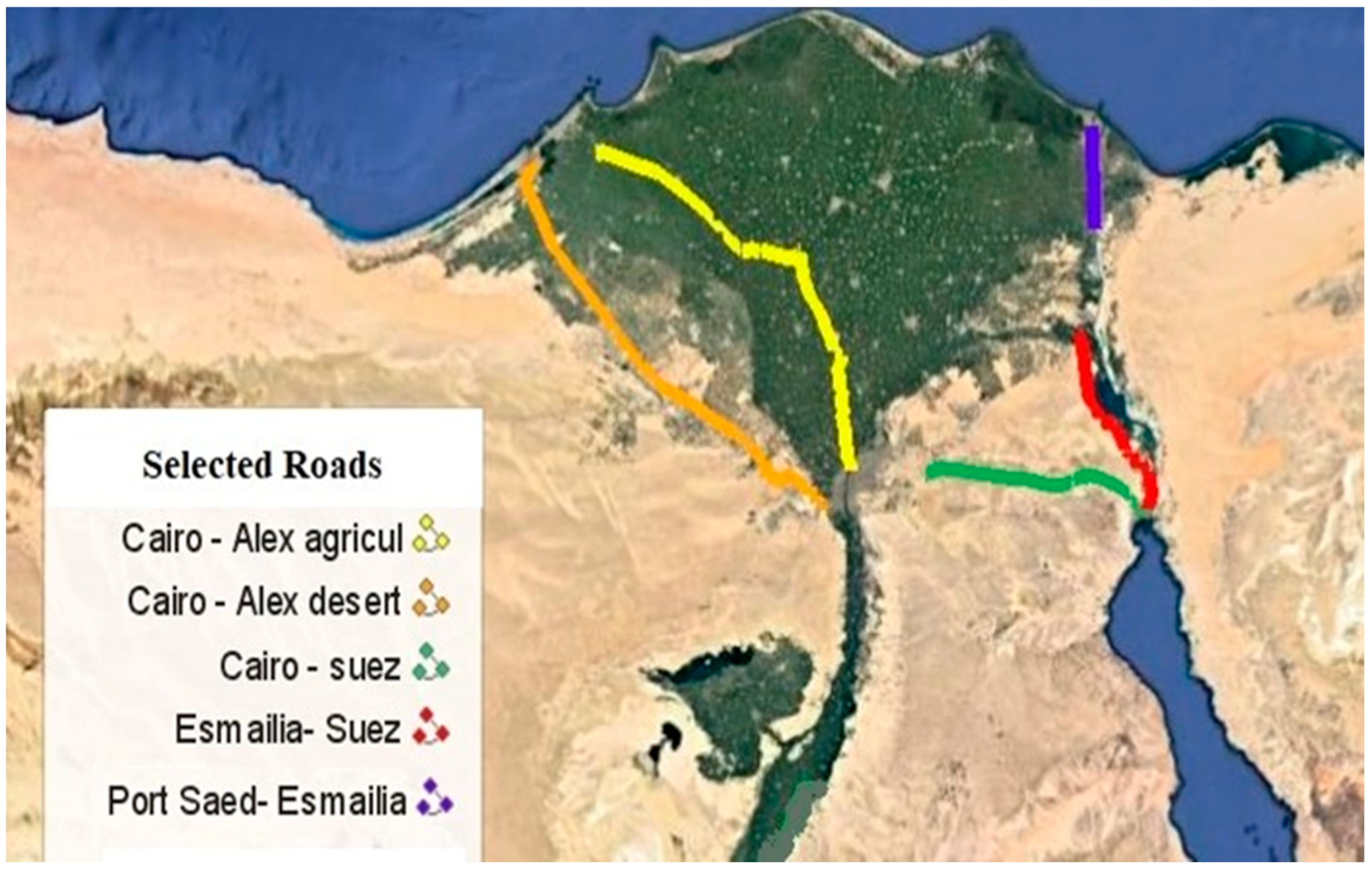
RD1	Cairo- Alexandria agriculture road	50
RD2	Cairo- Alexandria desert road	108
RD3	Cairo- Suez desert road	73
RD4	Ismailia-Port Said desert road	30
RD5	Ismailia-Suez desert road	61

. The geometric data obtained from the General Authority of Roads, Bridges, and Land Transport (GARBLT). This data consists of: (a) section length, (b) total pavement width in each direction, (c) median width, (d) shoulder width, (e) number of access points per section, (f) number of physical U-turns per section (g) number of lanes in each direction, and (h) the presence of curves along the section. Additionally, Google Earth maps were used to obtain missing geometric data. The data of crash frequencies for each kilometer and traffic volumes along the rural sections were obtained from GARBLT for four years (2008 to 2011). This data can be found in [4]. It is worth noting that GARBLT classify the roads to agricultural and desert roads based on the roadside activities (i.e., land use). The desert roads are the roads on which the main roadside activity is desert, while the agricultural roads are the ones on which the main roadside activity is Agriculture.

Four various segmentation approaches were used in this study [4]:

(1)

Sections with constant length, specifically, a length of one-kilometer (S1). This length was chosen as the crash data reported by GARBLT was available only for every kilometer;

(2)

Homogenous sections (S2): in this method, the highway length was divided into homogenous segments, as suggested by HSM [17] with respect to AADT and some geometric characteristics (e.g., number of lanes, median widths, shoulder width, etc.);

(3)

Segmentation based on curvature (S3): the highway was divided into two types of segments based on the presence of curves, as follows: (a) segments with curves, and (b) segments with no curves. It is worth mentioning that, as the crash data is reported every kilometer, the consecutive segments that contain curves are taken as one section and the consecutive one-kilometer sections with no curves are taken as one segment. This is done with respect to the AADT and other geometric characteristics; and

(4)

Segmentation based on curvature and U-turns (S4): the segments were categorized according to the presence of both curves and U-turns, as in S3. The consecutive segments with curves or U-turns were merged into one segment, and the consecutive sections without curves or U-turns were merged into one segment.

The number of sections for each road using the different segmentation methods along with the total crashes number per each year is presented in

Table 3. Crashes and number of sections based on the segmentation approach (Adapted with permission from [4], Springer Nature, 2020).

Road	Total Crashes/Year	Number of Sections
		S1	S2	S3	S4
RD1	271.75	50	16	28	30
RD2	46.75	108	21	51	55
RD3	47.50	73	31	41	48
RD4	69.0	30	13	13	21
RD5	24.0	61	34	44	40
Total	459.0	322	115	177	194

. It is worth noting that, the HSM procedure suggests that the minimum sample size desired for the calibration processes for each facility type is 30 to 50 sites, with 100 crashes at least per year [17]. From Table 3, none of the selected roads satisfies the HSM criteria needed for the calibration process regarding the number of sites and the total crashes per year except the first road (Cairo-Alexandria agriculture road) for S1 and S4. Thus, the data for all five roads were combined in one database to perform the calibration process.

Summary statistics describing the geometric elements and the AADT of the selected roads for the different segmentation methods are presented in

Table 4. Summary statistics of the selected roads geometric elements and AADT (Adapted with permission from [4], © Springer Nature, 2020).

Geometric Element	Maximum				Minimum				Mean
	Segmentation Method				Segmentation Method				Segmentation Method
	S1	S2	S3	S4	S1	S2	S3	S4	S1	S2	S3	S4
L (km) a	1.00	12.00	7.00	6.0	1.00	1.00	1.00	1.00	1.00	2.78	1.81	1.65
Accesses b	14	50	25	27	0	0	0	0	2.19	6.12	3.97	4.00
Uturn c	2.00	7.00	4.00	7.00	0.00	0.00	0.00	0.00	0.38	1.04	0.69	1.00
NHL d	2.00	5.00	5.00	5.00	0.00	0.00	0.00	0.00	0.34	0.95	0.61	1.00
AADT e	107,947				14,101				32,212
PW f	13				5.50				9.52
SW g	5.00				1.69				3.24
MW h	44.32				1.60				8.73
Nlanes i	4				2				3.05

^a L = Section length. ^b Accesses = Number of side access points. ^c Uturn = Number of U-turns. ^d NHL = Number of horizontal curves per section. ^e AADT = Average annual daily traffic (veh/day). ^f PW = Pavement width in each direction in meters. ^g SW = Shoulder width in meters.^h MW = Median width in meters. ⁱ Nlanes = Number of lanes in each direction.

.

2.2. Investigated SPFs

Table 5. The investigated international SPFs.

Model	SPF	Reference
HSM	$\mathrm{Ln}\left(\mathrm{N}\right)=-9.025+1.049\times \mathrm{Ln}\left(\mathrm{AADT}\right)+\mathrm{Ln}\left(\mathrm{L}\right)$	AASHTO [17]
Virginia	$\mathrm{Ln}\left(\mathrm{N}\right)=-7.47+0.88\times \ln (\mathrm{AAADT})+\ln (\mathrm{L})$	Kweon et al. [44]
North-Carolina	$\mathrm{Ln}(\mathrm{N})=-5.89+0.76\times \ln (\mathrm{AADT})+\ln (0.6214\times \mathrm{L})$	Srinivasan and Carter [45]
Alabama	$\mathrm{Ln}\left(\mathrm{N}\right)=-6.16+0.74\times \ln (\mathrm{AADT})+0.35\times \ln (0.6214\times \mathrm{L})$	Mehta & Lou [21]
Ohio	$\mathrm{Ln}\left(\mathrm{N}\right)=-9.709+1.125\times \ln (\mathrm{AADT})+\ln (0.6214\times \mathrm{L})-0.074\times \mathrm{SW}$	Farid et al. [46]
Italy (2012)	$\mathrm{Ln}(\mathrm{N})=-18.52+1.17\times \ln (\mathrm{AADT})+\ln (\mathrm{L})$	Cafiso et al. [47]
Italy (2017)	$\mathrm{Ln}\left(\mathrm{N}\right)=-19.19+1.24\times \ln (\mathrm{AADT})+\ln \left(\frac{\mathrm{L}}{1000}\right)$	Cafiso et al. [24]
Netherlands	$\mathrm{Ln}\left(\mathrm{N}\right)=-10.1934+0.4967\times \ln (\mathrm{AADT})+0.9647\times \ln (L)$	Reurings & Janssen [48]
Czech Rep.	$\begin{array}{ll}\mathrm{Ln}(\mathrm{N})=& -13.6468+0.9307\times \ln (\mathrm{AADT})+0.9499\times \ln (\mathrm{L})\\ & +0.42\times \mathrm{LES}+0.0004\times \mathrm{Curvature}\end{array}$	Šenk et al. [49]
Korea	$\mathrm{Ln}(\mathrm{N})=-15.245+\ln (\mathrm{AADT})+\ln (\mathrm{L})$	Choi et al. [50]
Ghana	$\mathrm{Ln}\left(\mathrm{N}\right)=-1.92+0.37\times \ln (\mathrm{AADT})+0.36\times \ln (\mathrm{L})$	Ackaah & Salifu [51]

L = Segment length (Kilometers); SW = Shoulder width (m); LW = lane width (m); LES = road vicinity (forest) [1 = yes]; Curvature = Number of curves in the road segment.

summarizes the investigated SPFs used in this study.

Five models are from the United States of America (USA): the HSM model, and four models from the states of Virginia, North Carolina, Alabama, and Ohio. Four models are from Europe: two models from Italy, and the other two from The Netherlands and the Czech Republic. Finally, the other two models are from Korea and Ghana, respectively.

2.3. Adjusting the Base Conditions

The base conditions of the international transferred SPFs were adjusted to accommodate local conditions in Egypt using three alternatives, namely: (1) default CMFs from the HSM; (2) locally derived CMFs; and (3) by recalibrating the constant term of the transferred SPF.

2.3.1. Default CMFs from the HSM

The HSM base conditions for the SPF for divided roadway segments on rural multilane highways are as follows:

(a)

Lane width (LW): 12 ft. (3.65 m),

(b)

Right shoulder width: 8 ft. (2.44 m),

(c)

Median width: 30 ft. (9.14 m),

(d)

Lighting: None, and

(e)

Automated speed enforcement: None.

If the local conditions are different from the HSM base conditions, then the corresponding CMFs which have been documented in the HSM for the changes should be applied. These CMFs can be obtained from the HSM (Equations (11)–(16) and (11)–(17), Tables 11–16 to 11–19) in the HSM) [17]. The HSM values were used to estimate the CMFs for lane width, median width, and right shoulder width only, as the automated speed enforcement was not applied on the roads under study, and the lightening information was not available in the collected data from GARBLT. Hence, the CMFs for both of the auto speed enforcement and lightening are equal to one for all segments.

2.3.2. Locally Derived CMFs Values

In this study, the local CMFs were derived using pre-developed jurisdiction cross-sectional SPFs, using the four pre-mentioned segmentation approaches [4]. The best-developed jurisdictions cross-sectional SPF is as follow (values between brackets [] represent the standard error) [4]:

$$\begin{array}{ll}\mathrm{N}=& \exp \left(\begin{array}{l}-13.62[1.09]+1.62[0.12]\times \ln (\mathrm{AADT})+1.54[0.13]\ln (\mathrm{L})-0.22[0.10]\times \mathrm{SW}+\\ t-0.21[0.03]\times \mathrm{PW}-0.08\left[0.02\right]\times \mathrm{Accesses}-0.44[0.13]\times \mathrm{HL}\end{array}\right)\\ & \mathrm{Degrees}\mathrm{of}\mathrm{Freedom}\left(\mathrm{DoF}\right)=698;\mathrm{Residual}\mathrm{Deviance}(\mathrm{RD})=634.77;\\ & AIC=2167.60;2LL=-2145.57;\mathrm{Shape}\mathrm{Parameter}(1/\mathrm{k})=0.68[0.07].\end{array}$$

(3)

where N = Predicted number of crashes (crashes/year); AADT = Average annual daily traffic (vehicle/day); L = Segment length (Km); t_i = Time trend effect (t₂₀₀₈, t₂₀₀₉, t₂₀₁₀, t₂₀₁₁); SW = Shoulder width (m); PW = Pavement width in each direction (m); Accesses = Number of side accesses per section and HL = Categorized variable, yes if the section contains a horizontal curve, and No otherwise.

The pre-developed jurisdiction SPF was then used to derive local CMFs, as follows [52]:

$${\mathrm{CMF}}_{\mathrm{x},\mathrm{i}}=\exp [{\mathsf{\beta }}_{\mathrm{i}}\times (\mathrm{X}-{\mathrm{X}}_{0,\mathrm{i}})]$$

(4)

where CMF_x,i = CMF specific to variable i with value of x; β_i = estimated coefficient for variable i; X = value of variable i, such as lane width, median width, shoulder width and X_0,i = base condition defined for variable i. 12ft (3.65 m) for lane width, 30ft (9.14 m) for median width, 8ft (2.44 m) for shoulder width, and zero for the presence of HL curve and accesses.

Table 6. Locally derived CMFs.

CMFi	Value
CMFSW	$e^{-0.22\times \left(\mathrm{SW}-2.44\right)}$
CMFPW	$e^{-0.21\times (\mathrm{PW}-\mathrm{N}*3.65)}$
CMFAccesses	$e^{-0.08\times (\mathrm{Accesses})}$
CMFHL	$e^{-0.44\times (\mathrm{HL})}$

presents the locally derived CMFs based on the pre-developed SPF.

The pre-developed cross-sectional model showed that shoulder width, pavement width, and the presence of either horizontal curves or accesses have a significant effect on crash occurrence, so the CMFs of these variables were developed to evaluate its effect on crash reduction as shown in Table 6. For example, for the shoulder width, the base case is assumed to be a shoulder width of 2.44 m (8 ft), which would translate to a CMF of 1. CMFs for varying shoulder width can be estimated by comparing their safety to the safety at a shoulder width of 2.44 m. For instance, for a shoulder width of 3 m, the CMF for total crashes would be about 0.88 (12% reduction in crashes).

2.3.3. Recalibrating the Constant Term and the Over-Dispersion Parameter of the Transferred SPF

The main advantage of recalibrating the constant term of the transferred SPF is that it allows the transferred SPF to accommodate local conditions as the model constant takes into consideration most factors outside the explanatory variables [14]. In this paper, the R-statistical software [53] was used to recalibrate the over-dispersion parameter and the constant of the transferred SPFs using the same approach by Sawalha and Sayed [14]. In this procedure, the constant of the transferred SPFs is recalibrated using the maximum likelihood method. The R-statistical software was used to recalibrate both of the overdispersion parameter and the constant of the transferred model by forcing the coefficient of the variables of the transferred model to remain constant with the same values in the transferred model. For all the three alternatives it is important to recalibrate the over-dispersion parameter (k) of the transferred SPFs before testing the SPFs transferability. The over-dispersion parameter is an indication of the variability of the model compared with the Poisson distribution with the same mean. The lower the value of the over-dispersion coefficient (k), the higher the accuracy of the resulting models [14].

2.4. Recalibrating the Over-Dispersion Parameter

The overdispersion parameter (k) of the transferred model was recalibrated using local data to allow the models to better suit local conditions in Egypt using the maximum likelihood procedure. This is the most widely used procedure [54]. Two alternatives were applied in recalibrating the over-dispersion parameter (k) of the transferred models. The first approach assumes that the over-dispersion parameter of the transferred models is fixed for all locations, while the second approach assumes that this over-dispersion parameter varies with the segment length. The difference between the two approaches was assessed by estimating the standard deviation of the Cr value of the transferred SPFs.

2.4.1. Constant Over-Dispersion Parameter

The log-likelihood function based on the Negative Binomial used in estimating the model parameters is as follows [55]:

$$\ln \left[{\mathrm{l}*(\mathsf{\beta }}_0{,\mathsf{\beta }}_1,\dots ,\mathrm{b})\right]={\displaystyle \sum _{\mathrm{i}=1}^{\mathrm{n}}\left[\begin{array}{l}\ln \mathsf{\Gamma }\left({\mathrm{obs}}_{\mathrm{i}}+\mathrm{b}\right)-\ln \mathsf{\Gamma }\left(\mathrm{b}\right)+\mathrm{bln}\left(\mathrm{b}\right)+\\ {\mathrm{obs}}_{\mathrm{i}}\ln \left({\mathrm{pred}}_{\mathrm{i}}\right)-\left({\mathrm{b}+\mathrm{obs}}_{\mathrm{i}}\right)\ln \left({\mathrm{b}+\mathrm{pred}}_{\mathrm{i}}\right)\end{array}\right]}$$

(5)

where obs_i = observed crashes on segment i; pred_i = predicted crashes on segment i; β₀, β1, …, b = parameter estimates of the model coefficients; b = inverse of the overdispersion parameter (shape parameter or b =1/k); and k = overdispersion parameter.

The recalibrated over-dispersion parameter of the prediction model is calculated as the value that maximizes the sum of $\ln \left[{\mathrm{l}*(\mathsf{\beta }}_0{,\mathsf{\beta }}_1,\dots ,\mathrm{b})\right]$.

2.4.2. Over-Dispersion Parameter as a Function of the Segment Length

In this case, k will vary for each location, and the value of “k*L” is calculated as the value that maximizes the sum of $\ln \left[{\mathrm{l}*(\mathsf{\beta }}_0{,\mathsf{\beta }}_1,\dots ,\mathrm{b})\right]$ as follows [55]:

$$\ln \left[{\mathrm{l}*(\mathsf{\beta }}_0{,\mathsf{\beta }}_1,\dots ,\mathrm{b})\right]={\displaystyle \sum _{\mathrm{i}=1}^{\mathrm{n}}\left[\begin{array}{l}\ln \mathsf{\Gamma }\left({\mathrm{obs}}_{\mathrm{i}}{+\mathrm{b}*\mathrm{L}}_{\mathrm{i}}\right)-\ln \mathsf{\Gamma }\left({\mathrm{b}*\mathrm{L}}_{\mathrm{i}}\right){+\mathrm{b}*\mathrm{L}}_{\mathrm{i}}\ln \left({\mathrm{b}*\mathrm{L}}_{\mathrm{i}}\right)+\\ {\mathrm{obs}}_{\mathrm{i}}\ln \left({\mathrm{pred}}_{\mathrm{i}}\right)-\left({\mathrm{b}*\mathrm{L}}_{\mathrm{i}}{+\mathrm{obs}}_{\mathrm{i}}\right)\ln \left({\mathrm{b}*\mathrm{L}}_{\mathrm{i}}{+\mathrm{pred}}_{\mathrm{i}}\right)\end{array}\right]}$$

(6)

where b = inverse of the overdispersion parameter (shape parameter or b = 1/k) and L_i = segment length i.

2.5. Goodness-of-Fit (GOF) Measures

In this analysis, five GOF measures are used to compare the performances of the international transferred SPFs, namely: (1) the mean absolute deviation (MAD); (2) the mean prediction bias (MPB); (3) the mean absolute percentage error (MAPE); (4) Pearson χ² statistic; and (5) Z-score.

2.5.1. The Mean Absolute Deviation (MAD)

MAD gives an indication of the average magnitude of variability in the model. Smaller values of MAD are preferred to larger ones [56]. The MAD is given by:

$$\mathrm{MAD}=\frac{{\displaystyle \sum _{\mathrm{i}=1}^{\mathrm{n}}\left|{\hat{\mathrm{Y}}}_{\mathrm{i}}{-\mathrm{Y}}_{\mathrm{i}}\right|}}{\mathrm{n}}$$

(7)

where n = sample size; ${\hat{\mathrm{Y}}}_{\mathrm{i}}$ = predicted crashes for site i; and Y_i = observed crashes for site i.

2.5.2. The Mean Prediction Bias (MPB)

MPB gives a knowledge into the average model bias compared to the observed data. If the model, does not over/under predict observations, the estimation of MPB will be zero [56]. The MPB is given by:

$$\mathrm{MAD}=\frac{{\displaystyle \sum _{\mathrm{i}=1}^{\mathrm{n}}\left|{\hat{\mathrm{Y}}}_{\mathrm{i}}{-\mathrm{Y}}_{\mathrm{i}}\right|}}{\mathrm{n}}$$

(8)

2.5.3. The Mean Absolute Percentage Error (MAPE)

MAPE measures the deviation between predicted and observed values. The prediction would be better when the value of MAPE approach “zero” [57].

$$\mathrm{MAPE}=\frac{{\displaystyle \sum _{\mathrm{i}=1}^{\mathrm{n}}\left|{\hat{\mathrm{Y}}}_{\mathrm{i}}{-\mathrm{Y}}_{\mathrm{i}}\right|}}{{\displaystyle \sum _{\mathrm{i}=1}^{\mathrm{n}}{\mathrm{Y}}_{\mathrm{i}}}}$$

(9)

2.5.4. Pearson χ² Statistic

The Pearson χ² statistic is given by the following equation:

$${\mathsf{\chi }}_{\mathrm{P}}^2={{\displaystyle \sum _{\mathrm{i}=1}^{\mathrm{n}}\frac{\left[{\mathrm{y}}_{\mathrm{i}}{-\mathrm{E}}_{\mathrm{i}}\left(\mathrm{Y}\right)\right]}{\mathrm{Var}\left({\mathrm{Y}}_{\mathrm{i}}\right)}}}^2=\frac{{\left({\mathrm{y}}_{\mathrm{i}}{-\mathsf{\mu }}_{\mathrm{i}}\right)}^2}{{\mathsf{\mu }}_{\mathrm{i}}\left({1+\mathsf{\mu }}_{\mathrm{i}}/\mathrm{k}\right)}$$

(10)

where µ_i = the mean crash frequency at section i during the same time.

Pearson χ² statistic is a measure of the goodness of fit that tests if a definite SPF developed by using certain data set gives a reliable expectation for a different set of data [13]. In addition, if the SPF that is applied to a new data set is correct and the observations in the new data set are independent, then the expected value and the standard deviation of the Pearson χ² statistics are as follow [58]:

$$\mathrm{E}\left({\mathsf{\chi }}_{\mathrm{P}}^2\right)=\mathrm{N}$$

(11)

$$\mathsf{\sigma }\left({\mathsf{\chi }}_{\mathrm{P}}^2\right)=\sqrt{2\mathrm{N}\left(1+3/\mathrm{k}\right)+{\displaystyle \sum _{\mathrm{i}=1}^{\mathrm{N}}\frac{1}{{\mathsf{\mu }}_{\mathrm{i}}\left({1+\mathsf{\mu }}_{\mathrm{i}}/\mathrm{k}\right)}}}$$

(12)

where N = the number of observations in the new data set.

2.5.5. Z-Score

The score that measures how far the calculated ${\mathsf{\chi }}_P^2$ is from its expected value is called the Z-score and is estimated as follows [14]:

$$\mathrm{Z}=\frac{{\mathsf{\chi }}_{\mathrm{P}}^2-\mathrm{E}\left({\mathsf{\chi }}_{\mathrm{P}}^2\right)}{\mathsf{\sigma }\left({\mathsf{\chi }}_{\mathrm{P}}^2\right)}$$

(13)

The Z-score value can be used to test the transferability of the crash prediction model, as the values near zero support the transferred model [14].

3. Results

3.1. Default CMFs from HSM Versus Locally Derived CMFs

Table 7. Recalibrated overdispersion parameters and Calibration factors for the HSM model using HSM default CMFs and locally derived CMFs.

Variable	Segmentation Method
	S1	S2	S3	S4
Recalibrated overdispersion parameter (k)	2809	2579	2.965	2.713
Observed crashes	1836
Predicted crashes using HSM default CMFs	5695	5676	5678	5675
Calibration factor using HSM default CMFs (Cr)	0.322 a,b,c,g (0.066) *	0.323 a,d,e,g (0.127)	0.323 b,d,g (0.115)	0.323 c,e,g (0.102)
Predicted crashes using Local CMFs	4692	2488	3706	3823
Calibration factor using Local CMFs	0.391 a,b,c,g (0.081)	0.738 a,g (0.289)	0.495 b,g (0.176)	0.480 c,g (0.151)

* Values between parentheses () represent the standard deviation of the Cr. ^a The difference between S1 and S2 segmentation methods is statistically significant at the 5% SL. ^b The difference between S1 and S3 segmentation methods is statistically significant at the 5% SL. ^c The difference between S1 and S4 segmentation methods SPF is statistically significant at the 5% SL. ^d The difference between S2 and S3 segmentation methods SPF is statistically significant at the 5% SL. ^e The difference between S2 and S4 segmentation methods SPF is statistically significant at the 5% SL. ^f The difference between S3 and S4 segmentation methods SPF is statistically significant at the 5% SL. ^g The difference between the two methods for the same segmentation method is statistically significant at the 5% SL.

shows the values of the recalibrated over-dispersion parameter (k) along with the calibration factors (Cr) of the transferred HSM SPF, with the standard deviation of the Cr in Parentheses, derived from using the default HSM CMFs and the locally derived Egyptian CMFs for the total crashes (TCs) for each segmentation approach. It can be noticed that from Table 7, the k parameter for segmentation S2 is relatively lower than the other investigated segmentations, which may indicate higher reliability of this segmentation method. It is worth noting that, the values of the calibration factors using new local CMFs outperform the HSM default values for total crashes, which is consistent with the results of AL Kaaf and Abdel-Aty [29]. Furthermore, by comparing the results of the calibration factors using new local CMFs for each segmentation approach, it can be found that the calibration factor from segmentation S2 (Cr = 0.738) is higher than the other segmentation methods, which is expected as the HSM SPFs were developed using homogeneous sections. Finally, both calibration methods yielded calibration factors lower than one meaning that HSM base SPFs are overestimating the mean crash frequencies on rural multilane divided roads in Egypt for all segmentation approaches.

To examine the validity of differences between the values of the calibration factors derived from the investigated segmentation approaches, two tests were employed: (1) the analysis of variance (ANOVA) that shows the difference between the four segmentation methods and (2) the t-test that shows the difference between each pair of segmentation methods for each transferred SPF model [59]. The result of the ANOVA test for both the calibrated HSM SPF using the HSM default CMFs and the local CMFs values show a statistically significant difference between the values of the calibration factors, derived from the investigated segmentation approaches at the 99.99% level of confidence as the p-values are almost zero (i.e., 0.000). The t-test for the calibrated HSM using the default CMFs shows that the difference between each pair of segmentation approaches is statistically significant at the 5% significance level (SL) except, the difference between S3 and S4 which is not statistically significant at both the 5% and the 10% significance level (p-value = 0.458 > 0.1). Finally, the t-test was performed to investigate whether there is a significant difference between the calibrated HSM SPF using the HSM default CMFs and the local CMFs using the same segmentation method. The t-test results show a statistically significant difference between the calibrated HSM SPF using the HSM default CMFs and the local CMFs for each segmentation method at the 99.99% level of confidence as the p-values are 0.000, 0.000, 0.000, and 0.000 for S1, S2, S3, and S4, respectively.

3.2. Locally Derived CMFs Versus Recalibrating the Constant of the Transferred Models

The results of recalibrating the over-dispersion parameters of the investigated international SPFs and the total calibration factors with the standard deviation of the Cr in Parentheses () using the two different procedures are shown in

Table 8. The calibration factors estimate using the locally derived CMFs.

Model	Nobs.	S1			S2			S3			S4
		k	Npred.	Cr	k	Npred.	Cr	k	Npred.	Cr	k	Npred.	Cr
HSM	1836	2.809	4692	0.391 a,b,c (0.081) *	2.580	2488	0.738 a (0.289)	2.966	3706	0.495 b (0.176)	2.713	3823	0.480 c (0.151)
Virginia		2.551	3760	0.488 a,b,c (0.096)	2.379	1997	0.919 a (0.346)	2.714	2965	0.619 b (0.210)	2.475	3055	0.601 c (0.181)
N. Carolina		3.210	5506	0.333 a,b,c (0.073)	3.004	2931	0.626 a (0.265)	3.537	4338	0.423 b (0.164)	3.099	4467	0.411 c (0.138)
Alabama		2.972	5636	0.326 a,b,c (0.069)	2.229	1305	1.406 a,d,e (0.516)	3.499	2487	0.738 b,d (0.284)	2.564	2792	0.658 c,e (0.201)
Ohio		1.812	2436	0.754 a,b,c (0.125)	1.675	1302	1.410 a (0.446)	1.934	1945	0.944 b (0.271)	1.784	1996	0.920 c (0.235)
Italy (2012)		1.657	2039	0.901 a,b,c (0.143)	1.611	1082	1.697 a (0.526)	1.800	1613	1.138 b (0.315)	1.741	1665	1.103 c (0.278)
Italy (2017)		1.752	2177	0.843 a,b,c (0.138)	1.634	1156	1.588 a (0.496)	1.838	1725	1.065 b (0.298)	1.775	1781	1.031 c (0.263)
Netherlands		1.966	1914	0.959 a,b,c (0.166)	1.852	990	1.854 a (0.616)	2.050	1469	1.250 b (0.369)	1.892	1519	1.209 c (0.318)
Czech		2.987	5045	0.364 a,b,c (0.077)	2.708	2527	0.727 a (0.292)	3.122	3834	0.479 b (0.174)	2.854	3982	0.461 c (0.149)
Korea		3.921	8958	0.205 a,b,c (0.050)	3.606	4752	0.386 a (0.179)	4.083	7072	0.260 b (0.108)	3.764	7292	0.252 c (0.093)
Ghana		2.323	2593	0.708 a (0.133)	2.188	761	2.413 a,d,e (0.871)	2.440	1388	1.323 d (0.426)	2.148	1554	1.181 e (0.331)

* Values between parentheses () represent the standard deviation of the Cr. ^a The Difference between S1 and S2 methods for the same transferred SPF is statistically significant at the 5% SL. ^b The difference between S1 and S3 methods for the same transferred SPF is statistically significant at the 5% SL. ^c The difference between S1 and S4 methods for the same transferred SPF is statistically significant at the 5% significance level. ^d The difference between S2 and S3 methods for the same transferred SPF is statistically significant at the 5% SL. ^e The Difference between S2 and S4 methods for the same transferred SPF is statistically significant at the 5% SL. ^f The Difference between S3 and S4 methods for the same transferred SPF is statistically significant at the 5% SL. ^g The Difference between the HSM-The Netherlands models for the S1 method is statistically significant at the 5% SL. ^h The difference between the Alabama-Virginia models for the S2 method is statistically significant at the 5% SL. ⁱ The Difference between the Korea-Ohio models for the S3 method is statistically significant at the 5% SL. ^j The Difference between the Czech-Italy (2017) models for the S4 method is statistically significant at the 5% SL.

and

Table 9. Calibration factors estimates by recalibrating the constant of the transferred SPFs.

Model	S1			S2			S3			S4
	New Constant	k	Cr	New Constant	k	Cr	New Constant	k	Cr	New Constant	k	Cr
HSM	−10.202	1.605	1.134 a,b,c	−10.17	1.593	1.102 a,d,e	−10.306	1.628	1.263 b,d	−10.146	1.694	1.076 c,e
			(0.177) *			(0.334)			(0.332)			(0.265)
Virginia	−8.458	1.642	1.184 a,b,c	−8.455	1.561	1.185 a,d,e	−8.575	1.65	1.335 b,d	−8.423	1.687	1.147 c,e
			(0.187)			(0.362)			(0.354)			(0.282)
N. Carolina	−7.278	1.688	1.202 a,b,c	−7.295	1.593	1.228 a,d,e	−7.426	1.691	1.4 b,d	−7.256	1.788	1.181 c,e
			(0.193)			(0.379)			(0.375)			(0.138)
Alabama	−7.394	1.697	1.204 a,b,c	−9.41	1.564	1.141 a,d,e	−7.094	2.078	1.4 b,d	−7.091	1.799	1.308 c,e
			(0.194)			(0.346)			(0.416)			(0.335
Ohio	−10.219	1.581	1.154 a,b,c	−10. 191	1.642	1.130 a,d,e	−10.323	1.538	1.285 b,d	−10. 172	1.546	1.104 c,e
			(0.176)			(0.331)			(0.329)			(0.263)
Italy (2012)	−18.826	1.568	1.084 a,b,c	−18.774	1.542	1.031 a,d,e	−18.937	1.62	1.214 b,d	−18.757	1.669	1.014 c,e
			(0.168)			(0.313)			(0.319)			(0.251)
Italy (2017)	−19.545	1.605	1.05 a,b,c	−19.481	1.549	0.987 a,d,e	−19.639	1.627	1.156 b,d	−19.467	1.685	0.974 c,e
			(0.164)			(0.3)			(0.304)			(0.242)
Netherlands	−10.5	1.865	1.195 a,b,c	−10.531	1.741	1.296 a,d,e	−10.621	1.861	1.393 b,d	−10.498	1.792	1.227 c,e
			(0.201)			(0.418)			(0.392)			(0.314)
Czech	−14.921	1.627	1.172 a,b,c	−14.867	1.556	1.19 a,d,e	−15.006	1.653	1.333 b,d	−14.861	1.699	1.147 c,e
			(0.184)			(0.363)			(0.353)			(0.282)
Korea	−17.081	1.612	1.157 a,b,c	−17.057	1.553	1.128 a,d,e	−17.189	1.629	1.287 b,d	−17.031	1.691	1.099 c,e
			(0.18)			(0.342)			(0.338)			(0.27)
Ghana	−2.51	1.979	1.166 a,b,c	−1.933	2.188	1.372 a,d,e	−2.23	2.348	1.359 b,d	−2.234	2.053	1.279 c,e
			(0.202)			(0.495)			(0.429)			(0.35)

* Values between parentheses () represent the standard deviation of the Cr. ^a The difference between S1 and S2 methods for the same transferred SPF is statistically significant at the 5% SL. ^b The difference between S1 and S3 methods for the same transferred SPF is statistically significant at the 5% SL. ^c The difference between S1 and S4 methods for the same transferred SPF is statistically significant at the 5% SL. ^d The difference between S2 and S3 methods for the same transferred SPF is statistically significant at the 5% SL. ^e The difference between S2 and S4 methods for the same transferred SPF is statistically significant at the 5% SL. ^f The difference between S3 and S4 methods for the same transferred SPF is statistically significant at the 5% SL. ^g The difference between the Netherlands-Italy (2017) models for the S1 method is statistically significant at the 5% SL. ^h The difference between the Ghana-Italy (2017) models for the S2 method is statistically significant at the 5% SL. ⁱ The difference between the Alabama-Italy (2017) models for the S3 method is statistically significant at the 5% SL. ^j The difference between the Alabama-Italy (2012) models for the S4 method is statistically significant at the 5% SL.

, respectively. It can be seen from Table 8 that, for the S1 segmentation method, the Netherlands and Italy (2012) models are the best models, as they lead to the best calibration factors of 0.959 and 0.901 (i.e., close to one). For the S2 segmentation method, the Virginia model is the best (Cr = 0.919). For the S3 segmentation method, Ohio, Italy (2017), and Italy (2012) models are the best models (Cr = 0.944, 1.065, 1.138, respectively). For the S4 segmentation method, the Italy (2017), Ohio, and Italy (2012) models are the best models (Cr =1.031, 0.920, 1.103, respectively). Additionally, the calibrated Italian SPF models using the locally derived CMFs have the lowest over-dispersion parameters.

Table 9 shows that for the S1 segmentation method, the Italy (2017) and Italy (2012) models are the best models, as they lead to the best calibration factors of 1.050 and 1.084 (i.e., close to one). For the S2 segmentation method, the Italy (2017) and Italy (2012) models are the best models (Cr = 0.987 and 1.031, respectively). For the S3 segmentation method, Italy’s (2017) model is the best (Cr = 1.156). For the S4 segmentation method, Italy (2012) and Italy (2017) models are the best models (Cr =1.014, 0.974, respectively).

By comparing between Table 8 and Table 9, it can be noticed that the recalibrated k parameters for the transferred models with recalibrated constant are lower than those estimated from the locally derived CMFs, which may indicate higher reliability of this transfer alternative. Additionally, the calibration factors for the transferred models with calibrated constant are outperforming the transferred models calibrated using the locally derived CMFs.

Additionally, the ANOVA and t-test were performed to investigate whether there is a significant difference among all the calibrated international SPFs for each segmentation approach. For example, the result of the t-test for the calibrated Alabama SPF using the locally derived CMFs shows that the difference between each pair of segmentation approaches is statistically significant at the 5% significance level except, the difference between S3 and S4 which is not statistically significant at both the 5% and the 10% significance level (p-value = 0.745 > 0.1), and the result of the ANOVA test shows that the difference between the calibrated international SPFs using the locally derived CMFs for all segmentation methods is statistically significant at the 99.99% level of confidence, as the P-values are almost zero (i.e., 0.0000) for all segmentation methods.

Finally, the t-test was performed to investigate whether there is a significant difference between each pair of the calibrated international SPFs for each segmentation method. For example, the t-test results show that for the S1 segmentation method, the difference between the calibrated HSM and the calibrated Netherlands model using the locally derived CMFs is statistically significant at the 5% level of significance (p-value = 0.000).

Table 10. Goodness of fit results of the transferred international SPFs.

S1 Segmentation Method
SPF Model	MAD		MBP		MAPE		χp2		σ(χp2)		Z−score
	Local CMFs	New Constant	Local CMFs	New Constant	Local CMFs	New Constant	Local CMFs	New Constant	Local CMFs	New Constant	Local CMFs	New Constant
HSM	10.717	4.781	8.870	−0.673	1.880	0.838	71.423	293.208	77.922	61.315	−3.216	−0.469
Virginia	9.094	5.013	5.977	−1.180	1.595	0.836	76.460	285.254	74.656	61.886	−3.289	−0.594
N. Carolina	13.146	5.069	11.398	−0.960	2.306	0.889	66.012	287.028	82.738	62.583	−3.094	−0.559
Alabama	13.730	5.089	11.798	0.968	2.408	0.893	68.819	288.034	79.910	62.727	−3.168	−0.541
Ohio	6.583	4.675	1.864	−0.762	1.154	0.820	119.594	284.803	64.420	59.940	−3.142	−0.621
Italy (1)	5.946 *	4.670 **	0.630 *	−0.440 **	1.043 *	0.819 **	179.548	309.559	62.083	60.756	−2.295 *	−0.205 **
Italy (2)	5.996 **	4.624 *	1.060 **	−0.269 *	1.052 **	0.811 *	166.785	312.470	63.543	61.340	−2.443 **	−0.155 *
Netherlands	6.604	5.363	1.243	−0.930	1.158	0.940	70.159	290.670	76.888	62.895	−3.275	−0.498
Czech Rep.	11.708	4.902	9.965	−0.837	2.053	0.860	68.558	286.699	80.092	61.657	−3.164	−0.573
Korea	22.356	4.832	22.118	−0.749	3.921	0.848	60.885	289.918	90.667	61.422	−2.880	−0.522
Ghana	7.868	5.533	2.352	−0.811	1.380	0.970	122.362	348.290	71.650	66.895	−2.786	0.393
S2 Segmentation Method
HSM	12.885	9.601	4.530	−1.182	1.011	0.753	26.560	93.582	44.837	44.837	−1.972	−0.595
Virginia	12.567	9.945	1.120	−1.993	1.986	0.780	27.613	90.811	43.261	43.261	−2.020	−0.668
N. Carolina	15.858	10.161	7.607	−2.369	1.244	0.797	24.716	90.754	47.986	47.986	−1.881	−0.664
Alabama	12.462	9.762	−3.685	−1.576	0.977	0.766	36.286	91.967	42.048	42.048	−1.872	−0.639
Ohio	10.993	9.400	−3.708	−1.463	0.862	0.737	37.252	89.532	40.610	40.610	−1.997	−0.727
Italy (1)	10.689 **	9.382 **	−5.238 **	−0.389 **	0.838 **	0.736 **	60.680	96.620	36.662	36.662	−1.482 *	−0.510 **
Italy (2)	10.581 *	9.270 *	−4.721 *	0.163 *	0.830 *	0.727 *	58.974	98.557	36.878	36.878	−1.519 **	−0.455 *
Netherlands	11.458	10.648	−5.871	−2.915	0.899	0.835	53.716	90.094	38.844	38.844	−1.578	−0.714
Czech Rep.	13.701	9.782	4.802	−2.036	1.075	0.767	25.797	90.919	45.812	45.812	−1.947	−0.666
Korea	22.514	9.708	20.253	−1.450	1.766	0.761	23.369	92.521	52.135	52.135	−1.758	−0.624
Ghana	11.992	11.458	−7.473	−3.459	0.941	0.899	47.923	93.439	36.719	36.719	−1.826	−0.604
S3 Segmentation Method
HSM	15.037	7.992	10.566	−2.162	1.450	0.770	37.719	149.175	59.196	45.636	−2.353	−0.610
Virginia	13.547	8.252	6.379	−2.605	1.306	0.796	39.276	144.694	56.894	45.965	−2.421	−0.703
N. Carolina	18.660	8.394	14.137	−2.964	1.799	0.809	35.295	151.525	62.883	46.432	−2.253	−0.549
Alabama	13.714	9.175	3.676	−2.963	1.322	0.885	43.441	144.405	58.054	46.634	−2.301	−0.699
Ohio	10.445	7.882	1.615	−2.301	1.007	0.760	54.672	144.180	49.097	44.680	−2.492	−0.735
Italy (1)	9.585 **	7.773 **	−1.259 **	−1.826 **	0.924 **	0.749 **	75.859	158.888	47.636	45.643	−2.123 *	−0.397 **
Italy (2)	9.572 *	7.678 *	−0.629 *	−1.402 *	0.923 *	0.740 *	73.503	159.278	48.061	45.722	−2.153 **	−0.388 *
Netherlands	10.501	8.858	−2.072	−2.926	1.012	0.854	66.624	157.078	52.324	48.321	−2.193	−0.412
Czech Rep.	16.198	8.209	11.288	−2.591	1.562	0.791	36.637	145.992	60.583	46.005	−2.317	−0.674
Korea	30.188	8.071	29.581	−2.313	2.910	0.778	29.039	147.401	68.488	45.691	−2.160	−0.648
Ghana	10.501	9.773	11.288	−2.738	1.059	0.942	71.171	117.476	48.486	78.527	−2.183	−0.758
S4 Segmentation Method
HSM	13.659	7.493	10.242	−0.668	1.443	0.792	43.319	163.096	59.548	48.158	−2.530	−0.642
Virginia	12.099	7.771	6.285	−1.213	1.278	0.821	45.698	155.991	57.180	48.196	−2.594	−0.789
N. Carolina	16.968	7.951	13.562	−1.454	1.793	0.840	40.068	153.741	63.209	48.439	−2.435	−0.831
Alabama	12.681	8.063	4.928	−2.228	1.340	0.852	46.082	164.059	58.077	49.858	−2.547	−0.601
Ohio	9.405	7.436	0.924	−0.890	0.994	0.776	72.072	158.497	49.672	46.845	−2.455	−0.758
Italy (2012)	8.748 **	7.347 **	−0.880 **	−0.130 *	0.924 **	0.776 **	109.561	169.772	49.178	48.355	−1.717 *	−0.501 **
Italy (2017)	8.720 *	7.263 *	−0.282 *	0.256 **	0.921 *	0.767 *	105.363	171.620	49.583	48.547	−1.788 **	−0.461 *
Netherlands	9.599	8.346	−1.636	−1.751	1.014	0.882	92.172	162.146	50.914	49.777	−2.000	−0.640
Czech Rep.	14.739	7.667	11.063	−1.213	1.557	0.810	41.700	156.258	60.910	48.108	−2.500	−0.785
Korea	28.439	7.572	28.126	−0.850	3.005	0.800	37.504	160.706	69.064	48.130	−2.266	−0.690
Ghana	10.024	8.566	−1.453	−2.065	1.059	0.905	96.587	124.462	53.758	52.720	−1.812	−1.319

* The best GOF values. ** The second best GOF values.

summarizes the GOF results of the investigated international SPFs to Egypt after the recalibration using the locally derived CMFs and by recalibrating the constant of the transferred international SPFs using the four segmentation methods. It can be noticed that the transferred SPFs with recalibrated the model constant have the lowest values of MAD, MPB, MAPE, and Z-score for all segmentation approaches. In addition, the transferred SPFs using segmentation method S1 have the best GOF results compared to the other segmentation methods. Additionally, the transferred Italian SPFs using the locally derived CMFs and by recalibrating the constant have the lowest values of MAD, MPB, MAPE, and Z-score for segmentation S1. For example, the MAD, MPB, MAPE, χ_p², and Z-score values for transferred Italy (2012) SPF by recalibrating the constant are 4.670, −0.440, 0.819, 309.559, and −0.205, respectively, compared to 5.946, 0.630, 1.043, 179.548 and −2.295, for the transferred Italy (2012) SPF using the locally derived CMFs. Moreover, the MAD, MPB, MAPE, χ_p², and Z-score values for transferred Italy (2017) SPF by recalibrating the constant are 4.624, −0.269, 0.811, 312.470, and −0.155, respectively, compared to 5.996, 1.060, 1.052, 166.785 and −2.443, for transferred Italy (2017) SPF using the locally derived CMFs.Thus, it can be concluded that the transfer of the SPFs with recalibrated model constant is superior to the transfer of the SPFs using the local CMFs, and the transferred Italian SPFs using segmentation method S1 predict crashes in Egypt reasonably well based on the GOF results.

3.3. Fixed Over-Dispersion Parameter Versus Variable Over-Dispersion Parameter

Table 11. The Calibration factors estimates using the locally derived CMFs with “fixed” and “variable” over-dispersion parameters.

Model	Segmentation S1		Segmentation S2		Segmentation S3		Segmentation S4
	Fixed k	Variable k	Fixed k	Variable k	Fixed k	Variable k	Fixed k	Variable k
HSM	0.391 (0.081) *	0.391 (0.081)	0.738 (0.289)	0.738 (0.266)	0.495 (0.176)	0.495 (0.128)	0.480 (0.151)	0.480 (0.117)
Virginia	0.488 (0.096)	0.488 (0.096)	0.919 (0.346)	0.919 (0.270)	0.619 (0.210)	0.619 (0.152)	0.601 (0.181)	0.601 (0.139)
N. Carolina	0.333 (0.073)	0.333 (0.073)	0.626 (0.265)	0.626 (0.204)	0.423 (0.164)	0.423 (0.116)	0.411 (0.138)	0.411 (0.106)
Alabama	0.326 (0.069)	0.326 (0.069)	1.406 (0.516)	1.406 (0.370)	0.738 (0.284)	0.738 (0.178)	0.658 (0.201)	0.658 (0.148)
Ohio	0.754 (0.125)	0.754 (0.125)	1.410 (0.446)	1.410 (0.365)	0.944 (0.271)	0.944 (0.199)	0.920 (0.235)	0.920 (0.182)
Italy (2012)	0.901 (0.143)	0.901 (0.143)	1.697 (0.526)	1.697 (0.417)	1.138 (0.315)	1.138 (0.234)	1.103 (0.278)	1.103 (0.212)
Italy (2017)	0.843 (0.138)	0.843 (0.138)	1.588 (0.496)	1.588 (0.343)	1.065 (0.298)	1.065 (0.221)	1.031 (0.263)	1.031 (0.201)
Netherlands	0.959 (0.166)	0.959 (0.166)	1.854 (0.616)	1.854 (0.480)	1.250 (0.369)	1.250 (0.272)	1.209 (0.318)	1.209 (0.247)
Czech Rep.	0.364 (0.077)	0.364 (0.077)	0.727 (0.292)	0.727 (0.226)	0.479 (0.174)	0.479 (0.126)	0.461 (0.149)	0.461 (0.114)
Korea	0.205 (0.050)	0.205 (0.050)	0.386 (0.179)	0.386 (0.139)	0.260 (0.108)	0.260 (0.078)	0.252 (0.093)	0.252 (0.072)
Ghana	0.708 (0.133)	0.708 (0.133)	2.413 (0.871)	2.413 (0.675)	1.323 (0.426)	1.323 (0.317)	1.181 (0.331)	1.181 (0.255)

* Values between parentheses () represent the standard deviation of the Cr.

summarizes the standard deviation of the calibration factor (SD (Cr)) of the recalibrated international SPFs using the locally derived CMFs using fixed over-dispersion parameter and variable over-dispersion parameter. Additionally,

Table 12. The Calibration estimates after recalibrating the constant with “fixed” and “variable” over-dispersion parameters.

Model	Segmentation S1		Segmentation S2		Segmentation S3		Segmentation S4
	Fixed k	Variable k	Fixed k	Variable k	Fixed k	Variable k	Fixed k	Variable k
HSM	1.134 (0.177) *	1.134 (0.177)	1.102 (0.334)	1.102 (0.263)	1.263 (0.332)	1.263 (0.253)	1.076 (0.265)	1.076 (0.201)
Virginia	1.184 (0.187)	1.184 (0.187)	1.185 (0.362)	1.185 (0.285)	1.335 (0.354)	1.335 (0.270)	1.147 (0.282)	1.147 (0.216)
N. Carolina	1.202 (0.193)	1.202 (0.193)	1.228 (0.379)	1.228 (0.299)	1.400 (0.375)	1.4 (0.288)	1.181 (0.138)	1.181 (0.226)
Alabama	1.204 (0.194)	1.204 (0.194)	1.141 (0.346)	1.141 (0.273)	1.400 (0.416)	1.4 (0.327)	1.308 (0.335)	1.308 (0.261)
Ohio	1.154 (0.176)	1.154 (0.176)	1.130 (0.331)	1.130 (0.262)	1.285 (0.329)	1.285 (0.251)	1.104 (0.263)	1.104 (0.201)
Italy (2012)	1.084 (0.168)	1.084 (0.168)	1.031 (0.313)	1.031 (0.247)	1.214 (0.319)	1.214 (0.243)	1.014 (0.251)	1.014 (0.190)
Italy (2017)	1.050 (0.164)	1.050 (0.164)	0.987 (0.300)	0.987 (0.206)	1.156 (0.304)	1.156 (0.232)	0.974 (0.242)	0.974 (0.183)
Netherlands	1.195 (0.201)	1.195 (0.201)	1.296 (0.418)	1.296 (0.330)	1.393 (0.392)	1.393 (0.300)	1.227 (0.314)	1.227 (0.245)
Czech Rep.	1.172 (0.184)	1.172 (0.184)	1.190 (0.363)	1.190 (0.285)	1.333 (0.353)	1.333 (0.271)	1. 147 (0.282)	1.147 (0.215)
Korea	1.157 (0.180)	1.157 (0.180)	1.128 (0.342)	1.128 (0.270)	1.287 (0.338)	1.287 (0.259)	1.099 (0.270)	1.099 (0.206)
Ghana	1.166 (0.202)	1.166 (0.202)	1.372 (0.495)	1.372 (0.384)	1.359 (0.429)	1.359 (0.336)	1.279 (0.350)	1.279 (0.279)

* Values between parentheses () represent the standard deviation of the Cr.

summarizes the standard deviation of the calibration factor (SD (Cr)) of the recalibrated international SPFs by recalibrating the constant using fixed over-dispersion parameter and variable over-dispersion parameter.

An examination of the tables indicates that using a variable over-dispersion parameter for the recalibrated SPFs is better than using fixed over-dispersion parameter, as the values of the standard deviation of the calibration factors of the recalibrated international SPFs with a variable over-dispersion parameter is lower than the standard deviation of the calibration factors of the recalibrated international SPFs with a Fixed over-dispersion parameter.

4. Discussion and Conclusions

This paper evaluated the transferability of HSM SPFs for total crashes on multilane divided rural roads in Egypt. As it is not an easy task to perform statistical crash modeling especially in developing countries, as it requires a considerable quantity of accurate data like recorded traffic volumes, geometric characteristics, and recorded crashes for several years. It will be useful if the SPFs produced for a specific area at a specific time can be used in a different time in the same or a different area as it will save time, effort, and money. The HSM SPFs was calibrated using both the HSM default CMFs values and local CMFs from a pre-developed Egyptian SPFs. Five Egyptian major rural roads with four-year crash data between 2008 and 2011were used in this research study. In addition, four different segmentation approaches were considered in this study, to compare the segmentation effect on transferability, namely: fixed segment length of one kilometer (S1); homogenous sections (S2); according to the presence of curvatures (S3); and according to the presence of curvatures and U-turns (S4).

The highway safety manual (HSM) models along with several international safety performance functions (SPFs) from United States of America, Europe, Netherlands, the Czech Republic, Korea, and Ghana were calibrated using the local CMFs from a pre-developed Egyptian SPFs and by recalibrating the constant of the transferred SPFs, to assess their suitability to represent crashes on Egyptian rural multilane highways.

The HSM transferability procedure was used in this analysis. The overdispersion parameter of the transferred models was firstly recalibrated to allow the transferred international SPFs to suit local conditions. The maximum likelihood method was presented for recalibrating the overdispersion parameter of the transferred international SPFs. Moreover, the t-test and ANOVA were used to investigate if the difference between the various segmentation approaches and among the calibrated models is statistically significant. In addition, five performance measures were used to assess the performance of the transferred models. These measures are the mean absolute deviation (MAD), the mean prediction bias (MPB), the mean absolute percentage error (MAPE), Pearson χ² statistic, and Z-score.

Based on the presented results and analyses, the main conclusions of this study are:

• The segmentation method was found to affect the performance of the transferred SPF model. The difference between the segmentation approaches and among the investigated international models is statistically significant at the 5% significance level.
• The total crashes calibration factors derived from both HSM default CMFs values and locally derived CMFs are lower than one, meaning that the HSM models are overestimating the crash occurrence on multilane rural divided roads in Egypt. Moreover, the calibrated HSM model using locally derived CMFs with the S2 segmentation method outperformed the calibrated HSM model using HSM default CMFs values;
• The calibrated Italian SPF using both locally derived CMFs and by recalibrating the constant outperformed all other investigated international SPFs, as they performed very well for all segmentation methods, especially, for the S1 segmentation method;
• The recalibration of the constant of the transferred models to allow it to better suit local conditions in Egypt is superior to the SPFs recalibration using the local CMFs;
• Using variable overdispersion parameter for the recalibrated SPFs outperforms the constant overdispersion parameter.

Study Limitations

In spite of the fact that this study introduced comprehensive examinations to evaluate the transferability of the international SPFs to Egypt; the main challenge of this study was the lack of recent crash data, and therefore crash data for the years 2008 to 2011 were used. The second challenge was the crash underreporting; Asal and Said [1] reported that less than half of the road crashes fatalities are reported to the police. Thus, crash underreporting is considered a major problem in safety analysis that requires quick solutions.

References

- Asal, H.I.; Said, D. An Approach for Development of Local Safety Performance Functions for Multi-Lane Rural Divided Highways in Egypt. Transp. Res. Rec. 2019, 2673, 510–521. [Google Scholar] [CrossRef]
- Herman, J.; Ameratunga, S.; Jackson, R.T. Burden of road traffic injuries and related risk factors in low and middle-income Pacific Island countries and territories: A systematic review of the scientific literature (TRIP 5). BMC Public Health 2012, 12, 479. [Google Scholar] [CrossRef] [Green Version]
- Ismail, M.A.; Abdelmageed, S.M.M. Cost of road traffic accidents in Egypt. World Acad. Sci. Eng. Technol. 2010, 42, 1308–1314. [Google Scholar]
- Elagamy, S.R.; El-Badawy, S.M.; Shwaly, S.A.; Zidan, Z.M.; Shahdah, U. Segmentation effect on developing safety performance functions for rural arterial roads in Egypt. Innov. Infrastruct. Solut. 2020, 5, 1–12. [Google Scholar] [CrossRef]
- Park, J.; Abdel-Aty, M.; Lee, J.; Lee, C. Developing crash modification functions to assess safety effects of adding bike lanes for urban arterials with different roadway and socio-economic characteristics. Accid. Anal. Prev. 2015, 74, 179–191. [Google Scholar] [CrossRef]
- Saleem, T. Advancing the Methodology for Predicting the Safety Effects of Highway Design and Operational Elements. Ph.D. Thesis, Ryerson University, Toronto, ON, Canada, 2016. [Google Scholar]
- Glavić, D.; MladenoviĆ, M.N.; Stevanovic, A.; Tubić, V.; Milenković, M.; Vidas, M. Contribution to Accident Prediction Models Development for Rural Two-Lane Roads in Serbia. PROMET Traffic Transp. 2016, 28, 415–424. [Google Scholar] [CrossRef] [Green Version]
- Claros, B.; Sun, C.; Edara, P. Missouri-Specific Crash Prediction Model for Signalized Intersections. Transp. Res. Rec. J. Transp. Res. Board 2018, 2672, 32–42. [Google Scholar] [CrossRef]
- Eenink, R.; Reurings, M.; Elvik, R.; Cardoso, J.; Wichert, S.; Stefan, C. Accident Prediction Models and Road Safety Impact Assessment: Recommendations for using these tools. RiPCORD iSEREST 2005, 506184, 1–20. [Google Scholar]
- Hauer, E.; Hakkert, A.S. Extent and some implications of incomplete accident reporting. Transp. Res. Rec. 1988, 1185, 1–10. [Google Scholar]
- Amoros, E.; Martin, J.-L.; Laumon, B. Under-reporting of road crash casualties in France. Accid. Anal. Prev. 2006, 38, 627–635. [Google Scholar] [CrossRef]
- Imprialou, M.-I.M.; Quddus, M. Crash data quality for road safety research: Current state and future directions. Accid. Anal. Prev. 2019, 130, 84–90. [Google Scholar] [CrossRef] [Green Version]
- Jacobs, G.; Sayer, I. Road accidents in developing countries. Accid. Anal. Prev. 1983, 15, 337–353. [Google Scholar] [CrossRef] [Green Version]
- Sawalha, Z.; Sayed, T. Transferability of accident prediction models. Saf. Sci. 2006, 44, 209–219. [Google Scholar] [CrossRef]
- Peden, M.; Scurfield, R.; Sleet, D.; Mohan, D.; Hyder, A.A. World Report on Traffic Injury Prevention: A Graphical Overview of the Global Burden of Injuries; WHO: Geneva, Switzerland, 2004. [Google Scholar]
- Srinivasan, R.; Carter, D.; Bauer, K. Safety Performance Function Decision Guide: SPF Calibration versus SPF Development (No. FHWA-SA-14-004); Federal Highway Administration, Office of Safety: Washington, DC, USA, 2013.
- Highway Safety Manual; American Association of State Highway and Transportation Officials: Washington, DC, USA, 2010.
- Sayed, T.; Leur, P. Collision Prediction Models for British Columbia; BC Ministry of Transportation & Infrastructure: Victoria, BC, Canada, 2008.
- Agostino, C.D. Investigating Transferability and Goodness of Fit of Two Different Approaches of Segmentation and Model form for estimating safety performance of Motorways. Procedia Eng. 2014, 84, 613–623. [Google Scholar] [CrossRef] [Green Version]
- Geni, B.B.; Hauer, E. User’s Guide to Develop Highway Safety Manual Safety Performance Function Calibration Factors; National Cooperative Highway Research Program: Washington, DC, USA, 2014. [Google Scholar]
- Mehta, G.; Lou, Y. Calibration and Development of Safety Performance Functions for Alabama. Transp. Res. Rec. J. Transp. Res. Board 2013, 2398, 75–82. [Google Scholar] [CrossRef]
- Saha, D.; Alluri, P.; Gan, A. A Bayesian procedure for evaluating the frequency of calibration factor updates in highway safety manual (HSM) applications. Accid. Anal. Prev. 2017, 98, 74–86. [Google Scholar] [CrossRef]
- Persaud, B.; Lord, D.; Palmisano, J. Calibration and Transferability of Accident Prediction Models for Urban Intersections. Transp. Res. Rec. J. Transp. Res. Board 2002, 1784, 57–64. [Google Scholar] [CrossRef] [Green Version]
- Cafiso, S.; Dágostino, C.; Persaud, B. Investigating the influence of segmentation in estimating safety performance functions for roadway sections. J. Traffic Transp. Eng. 2018, 5, 129–136. [Google Scholar] [CrossRef]
- Dissanayake, S.; Aziz, S.R. Calibration of the Highway Safety Manual and Development of New Safety Performance Functions for Rural Multilane Highways in Kansas (No. K-TRAN: KSU-14-3); Kansas Department of Transportation, Bureau of Research: Topeka, KS, USA, 2016. [Google Scholar]
- Sun, C.; Brown, H.; Edara, P.; Claros, B.; Nam, K. Calibration of the HSM’s SPFs for Missouri; Publication CMR14-007; Missouri Department of Transportation: Missouri, MO, USA, 2014.
- Young, J.; Park, P.Y. Benefits of small municipalities using jurisdiction-specific safety performance functions rather than the Highway Safety Manual’s calibrated or uncalibrated safety performance functions. Can. J. Civ. Eng. 2013, 40, 517–527. [Google Scholar] [CrossRef]
- Sacchi, E.; Persaud, B.; Bassani, M. Assessing International Transferability of Highway Safety Manual Crash Prediction Algorithm and Its Components. Transp. Res. Rec. J. Transp. Res. Board 2012, 2279, 90–98. [Google Scholar] [CrossRef]
- Al Kaaf, K.; Abdel-Aty, M. Transferability and Calibration of Highway Safety Manual Performance Functions and Development of New Models for Urban Four-Lane Divided Roads in Riyadh, Saudi Arabia. Transp. Res. Rec. J. Transp. Res. Board 2015, 2515, 70–77. [Google Scholar] [CrossRef]
- Brimley, B.K.; Saito, M.; Schultz, G.G. Calibration of Highway Safety Manual Safety Performance Function. Transp. Res. Rec. J. Transp. Res. Board 2012, 2279, 82–89. [Google Scholar] [CrossRef]
- Lu, J.; Haleem, K.; Alluri, P.; Gan, A. Full versus Simple Safety Performance Functions. Transp. Res. Rec. J. Transp. Res. Board 2013, 2398, 83–92. [Google Scholar] [CrossRef]
- Williamson, M.; Zhou, H. Develop Calibration Factors for Crash Prediction Models for Rural Two-Lane Roadways in Illinois. Procedia Soc. Behav. Sci. 2012, 43, 330–338. [Google Scholar] [CrossRef] [Green Version]
- Xie, F.; Gladhill, K.; Dixon, K.K.; Monsere, C.M. Calibration of Highway Safety Manual Predictive Models for Oregon State Highways. Transp. Res. Rec. J. Transp. Res. Board 2011, 2241, 19–28. [Google Scholar] [CrossRef]
- Fletcher, J.P.; Baguley, C.J.; Sexton, B.; Done, S. Road Accident Modelling for Highway Development and Management in Developing Countries. Main Report: Trials in India and Tanzania; Project Report No: PPR095; UK Department for International Development (DFID): London, UK, 2006.
- Hauer, E.; Persaud, B. Common Bias in Before-and After Accident Comparison and Its Elimination. Transp. Res. Rec. J. Transp. Res. Board 1983, 905, 164–174. [Google Scholar]
- Sun, X.; Li, Y.; Magri, D.; Shirazi, H. Application of Highway Safety Manual Draft Chapter: Louisiana Experience. Transp. Res. Rec. J. Transp. Res. Board 2006, 1950, 55–64. [Google Scholar] [CrossRef]
- Fitzpatrick, K.; Iv, W.S.; Carvell, J. Using the Rural Two-Lane Highway Draft Prototype Chapter. Transp. Res. Rec. 2007, 1950, 44–54. [Google Scholar] [CrossRef]
- Martinelli, F.; La Torre, F.; Vadi, P. Calibration of the Highway Safety Manual’s Accident Prediction Model for Italian Secondary Road Network. Transp. Res. Rec. J. Transp. Res. Board 2009, 2103, 1–9. [Google Scholar] [CrossRef]
- Koorey, G. Calibration of Highway Crash Prediction Models for Other Countries: A Case Study with IHSDM. In Proceedings of the 4th International Symposium on Highway Geometric Design, Valencia, Spain, 2–5 June 2010. [Google Scholar]
- Persaud, B.; Lyon, C.; Faisal, S.; Chen, Y.; James, B. Adoption of Highway Safety Manual methodologies for safety assessment of Canadian roads. In Proceedings of the 2012 Conference of the Transportation Association of Canada, Fredericton, NB, Canada, 14–17 October 2012. [Google Scholar] [CrossRef]
- Srinivasan, R.; Colety, M.; Bahar, G.; Crowther, B.; Farmen, M.; Information, R. Estimation of Calibration Functions for Predicting Crashes on Rural Two-Lane Roads in Arizona. Transp. Res. Rec. J. Transp. Res. Board 2016, 2583, 17–24. [Google Scholar] [CrossRef]
- Srinivasan, S.; Haas, P.; Dhakar, N.S.; Hormel, R.; Torbic, D.; Harwood, D. Development and Calibration of Highway Safety Manual Equations for Florida Conditions; Florida Department of Transportation Research Center: Tallahassee, FL, USA, 2011.
- Dixon, K.; Monsere, C.; Xie, F.; Gladhill, K. Calibrating the Highway Safety Manual Predictive Methods for Oregon Highways Final Report; Oregon Transportation Research and Education Consort: Portland, OR, USA, 2013. [Google Scholar]
- Kweon, Y.J.; Lim, I.K. Development of Safety Performance Functions for Multilane Highway and Freeway Segments Maintained by the Virginia Department of Transportation; (No. FHWA/VCTIR 14-R14); Virginia Center for Transportation Innovation and Research: Charlottesville, VA, USA, 2014. [Google Scholar]
- Srinivasan, R.; Carter, D. Development of Safety Performance Functions for North Carolina; (No. FHWA/NC/2010-09); North Carolina Department of Transportation Research and Analysis Group: Chapel Hill, NC, USA, 2011.
- Farid, A.; Abdel-Aty, M.; Lee, J. Transferring and calibrating safety performance functions among multiple States. Accid. Anal. Prev. 2018, 117, 276–287. [Google Scholar] [CrossRef] [PubMed]
- Cafiso, S.; Di Silvestro, G.; Di Guardo, G. Application of Highway Safety Manual to Italian Divided Multilane Highways. Procedia Soc. Behav. Sci. 2012, 53, 910–919. [Google Scholar] [CrossRef] [Green Version]
- Reurings, M.; Janssen, T. Accident Prediction Models for Urban and Rural Carriageways; Report R-2006-14; SWOV Institute for Road Safety Research: Leidschendam, The Netherlands, 2007. [Google Scholar]
- Šenk, P.; Ambros, J.; Pokorný, P.; Striegler, R. Use of Accident Prediction Models in Identifying Hazardous Road Locations. Trans. Transp. Sci. 2012, 5, 223–232. [Google Scholar] [CrossRef] [Green Version]
- Choi, E.; Kim, E.; Cho, H.; Yang, J. Development of a Korea highway safety evaluation proto type model on the concept of IHSDM crash prediction module. Int. J. Urban Sci. 2014, 18, 61–75. [Google Scholar] [CrossRef]
- Ackaah, W.; Salifu, M. Crash prediction model for two-lane rural highways in the Ashanti region of Ghana. IATSS Res. 2011, 35, 34–40. [Google Scholar] [CrossRef] [Green Version]
- Wu, L.; Lord, D.; Zou, Y. Validation of Crash Modification Factors Derived from Cross-Sectional Studies with Regression Models. Transp. Res. Rec. J. Transp. Res. Board 2015, 2514, 88–96. [Google Scholar] [CrossRef]
- R Development Core Team. R: A Language and Environment for Statistical Computing; R Foundation for Statistical Computing: Vienna, Austria, 2019. [Google Scholar]
- Lawless, J.F. Negative binomial and mixed poisson regression. Can. J. Stat. 1987, 15, 209–225. [Google Scholar] [CrossRef]
- Hauer, E. The Art of Regression Modeling in Road Safety; Springer: New York, NY, USA, 2015. [Google Scholar]
- Begum, S.M. Investigation of Model Calibration Issues in the Safety Performance Assessment of Ontario Highways. Ph.D. Thesis, Ryerson University, Toronto, ON, Canada, 2008. [Google Scholar]
- Qian, Y.; Zhang, X.; Fei, G.; Sun, Q.; Li, X.; Stallones, L.; Xiang, H. Forecasting deaths of road traffic injuries in China using an artificial neural network. Traffic Inj. Prev. 2020, 1–6. [Google Scholar] [CrossRef]
- Vogt, A.; Joe, B. Accident Models for Two-Lane Rural. Transp. Res. Rec. 2014, 1635, 18–29. [Google Scholar] [CrossRef]
- StatPages. Interactive Statistics—One-Way ANOVA from Summary Data. 2019. Available online: https://statpages.info/anova1sm.html (accessed on 12 November 2019).