What Employees Do Today Because of Their Experience Yesterday: How Incidental Learning Influences Train Driver Behavior and Safety Margins (A Big Data Analysis)

Abstract

Employee behavior plays an important role in the occurrence and prevention of incidents, affecting safety margins. In this study, we examine the potential impact of incidental learning on human behavior in the presence of variation in task design. Incidental learning is the day-to-day on-the-job learning that occurs unintentionally. This learning influences which behavior (schema) is more likely to be activated in the employee’s brain. We posit that an incorrect schema can be activated and lead to undesired behavior if the employee is often exposed to (visually) similar tasks that require different behavior. In rail transport, there is a risk of trains passing through red signals. The train driver’s behavior plays an important role in preventing these signal passed at danger (SPAD) incidents. In this study we used speed and location data to analyze train driver deceleration behavior during red signal approaches in the Netherlands. The Dutch rail system showed variation in yellow signal aspects and signal distance. An analysis using 19 months of empirical data indicated changes in behavior when the employee had been previously exposed to different behavior requirements in the same location with a similar yellow signal. These results imply that task design can be improved by taking into consideration what an employee is exposed to during other moments of the shift, and not just during the execution of the specific task.

1. Introduction

Incidents still occur, even in situations when rules and regulations are followed and organizations feel that they did everything they could to prevent them. One important element in incident causation and prevention is the behavior of employees at the “sharp end”. How can organizations support their employees in executing tasks as desired?

In this study, we look at the risk of a train passing through a red signal. A signal passed at danger (SPAD) event can lead to a derailment or collision. Even those SPAD events with negligible chances of derailment or collision incur costs in terms of delays, required reactive actions, and the emotional state of train drivers [1]. In 2019, there were 142 SPADs in the Netherlands [2]. Train driver behavior has a large influence on whether SPADs occur or not. Train drivers in the Netherlands are trained, tested, and experienced, and are fully aware of the risks involved during red aspect approaches. Many developments have also been made to improve the infrastructure to better fit the tasks of train drivers. The visibility of signals has for example been improved and care is taken that signals are not placed in confusing locations. There is however still some variation in train driving behavior that is not understood.

In this paper, we examine incidental learning as a factor impacting human behavior [3]. Incidental learning can have a positive or a negative impact. Incidental learning is the learning that occurs without an explicit intention [4]. It is the on-the-job learning that occurs, in contrast to learning during training sessions and courses. In experimental settings, a distinction between intentional learning and incidental learning is made depending on the instructions that participants are given. During the incidental learning condition, the participants are not aware of the learning situations and are not instructed as to what they will truly be tested on [5].

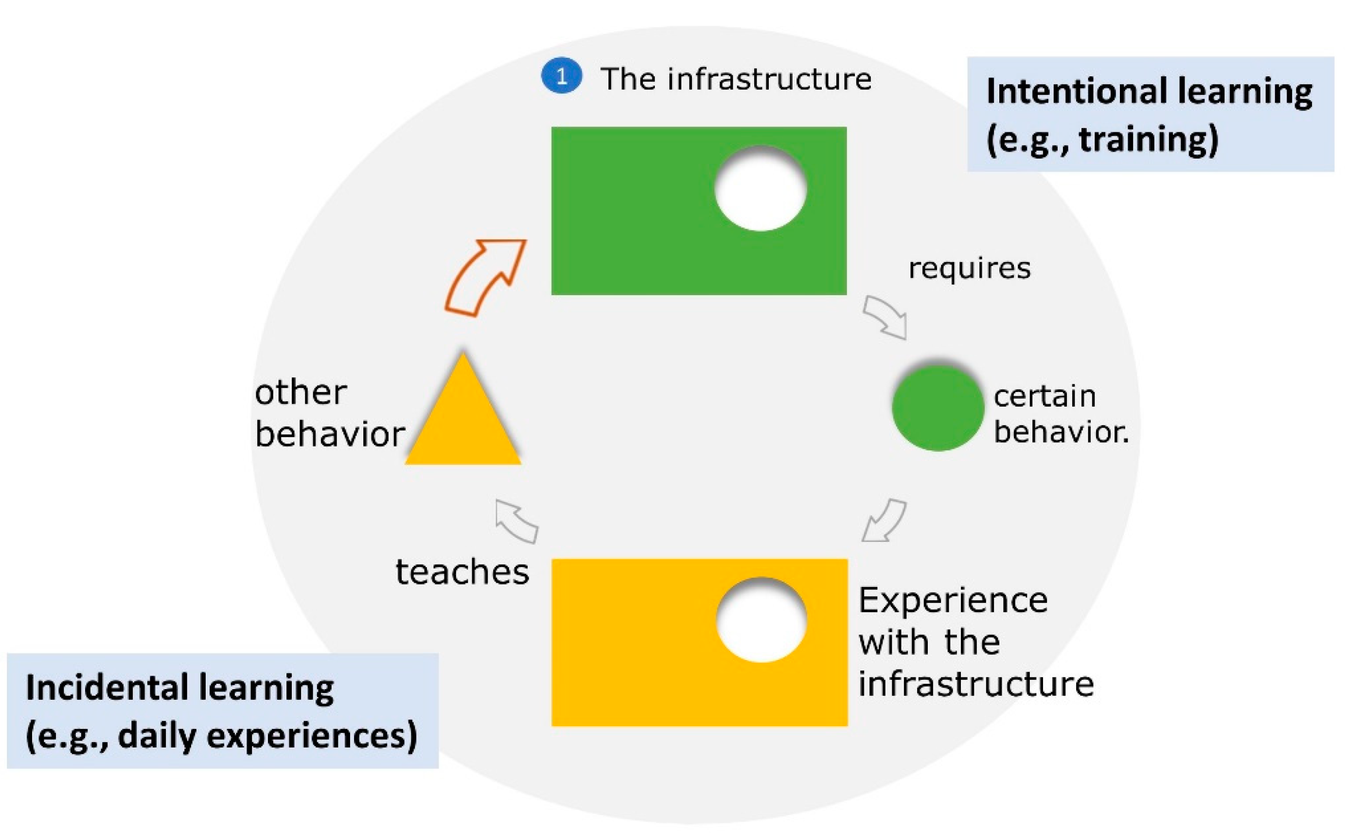
If there is indeed a significant negative influence of incidental learning, this is important to understand as it can undermine results of explicit training and awareness campaigns (See Figure 1). It is of course important to train employees (see top right of figure), but if incidental learning teaches employees different behavior (bottom left of figure), then this explicit training will be partly undone.

Incidental learning is difficult to identify as a cause for changes in human behavior. One reason for this is that incidental learning can be part of implicit learning. This means that the employee is not necessarily aware of what he or she has learned or even that he or she has learned. Implicitly learned knowledge can control action, but the learner himself is not able to tell others that this is what happened [6,7,8]. Wang and Theeuwes focus on implicit attentional bias and show that people quickly pick up on visual changes in the environment and change their behavior accordingly even though they are not aware of the changes. They conclude that “people adapt to a changing environment but that there are lingering biases from previous learned experiences that impact the current selection priorities” [9].

Another reason that incidental learning can be difficult to identify is that during an incident analysis, the situation at the time of the incident is analyzed. Whilst the causes of the situation might also be analyzed, the preceding “normal” situation is often not analyzed. Thus, what the employee or train driver is exposed to on a daily basis before the incident is not necessarily considered. Even when it is, it is hard to prove the impact of previous exposure, i.e., incidental learning. In the case of SPADs, there are simply not enough incidents to analyze this cause systematically without specific direction and detailed hypotheses. A third reason for difficulty of detecting incidental learning in the past may be small effect size.

1.1. Incidental Learning Influences the Schemas in an Employee’s Brain

Incidental learning influences the development and activation of schemas in an employee’s brain. Schemas embody the procedural knowledge that is needed to carry out actions [10,11,12]. Schemas can be described as generalized procedures for carrying out actions. In novel tasks, when a schema does not yet exist, much attention is needed to carry out the action. Once schemas are present, these actions can mostly be performed automatically, i.e., with little attention required. Schemas thus help us perform actions more efficiently [13]. Actions will be performed correctly if the right schema is activated at the right time.

Schemas can be activated in a top-down fashion via the intention to perform an action. This requires attention. Schemas can however also include triggering conditions. If the environmental conditions match the triggering conditions, then the schema can be activated without conscious thought. For example, if one has a cup nearby on the desk, he/she can pick it up and have a sip without explicit intention or even thirst. The mere sight of the glass can trigger the schema to pick it up (see Ref. [14,15] with respect to unconscious control of motor action; Ref. [16,17,18,19] specifically for hand movement). An event (a cue) can become a trigger for a schema when it is often paired with the execution of the schema. The more often they are paired, the stronger the schema activation will be upon perception of the cue. This linking of a cue to a schema is part of incidental learning.

Problems occur when the incorrect schema in one’s head is activated. Correct behavior is then activated, but it is unsuitable for the specific situation. We hypothesize that this is more likely to occur if there is variation in task design. Specifically, we posit that human error is more likely to occur if different behavior is required in (visually) similar settings. An example is crossing the street on foot. In right-driving countries, pedestrians should look left and right and left again, before crossing. When a pedestrian goes on holiday to a left-driving country, he or she should look right and left and then right again, but the pedestrian is inclined to look in the pattern he or she is used to, namely left–right–left. This is clearly not caused by a sudden lack of head turning ability, but caused by a different requirement in a similar situation (crossing a road). It can therefore occur even if the pedestrian is fully aware of the rules that apply in a given country and wishes to adhere to them (see e.g., research using the Stroop test for ample evidence of people erring in the simple task of naming a color because they read the colored word instead [20]). The same applies to driving a car. People are perfectly capable of taking a roundabout clockwise. They are also perfectly capable of taking a roundabout anti-clockwise. However, going on holiday and driving on the opposite side of the road than one is used to is very difficult the first few times. When there are other cars around, this is a visual reminder that one is in a different country and the roundabout should be taken the other way round. However, when there are no other cars in sight or there are other distracting traffic situations present, it is easy to veer into the old pattern and take a roundabout the wrong way round.

1.2. Application to Rail

During a red aspect approach, it is the train diver’s task to decelerate sufficiently to stop in front of the red aspect. The driver has schemas in his brain for the deceleration behavior. The signal aspects along the tracks provide information on which behavior is suitable. A red aspect is preceded by a yellow aspect to inform a train driver that a red aspect is coming and that he should start to decelerate. 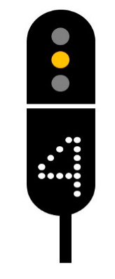In contrast to road transport, this is necessary because trains have a very long braking distance (e.g., 580 m at 140 km/h and an emergency deceleration of 1.3 m/s²). In the Dutch signaling system, the aspect sequence green–yellow–red is most common, but other yellow aspects are also used. A yellow aspect can for example be combined with a number. If the distance between the yellow and red signal is relatively short given the track speed, then the yellow signal can be preceded by, for example, yellow with the number four (yellow:4) (See Figure 2). In that case, the driver will have to reduce his/her speed and drive at 40 km/h or less by the next signal.

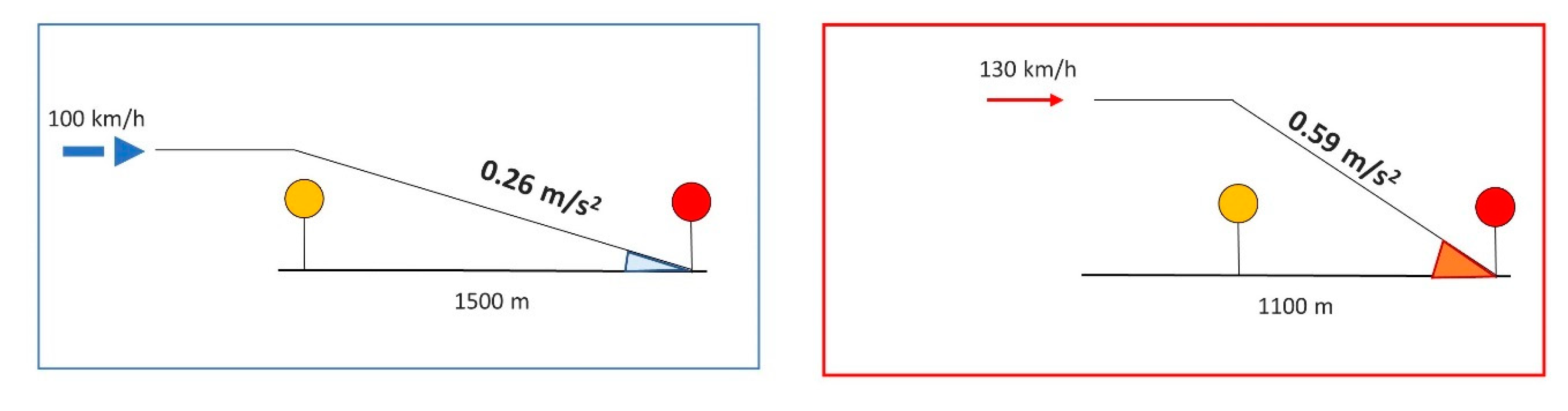
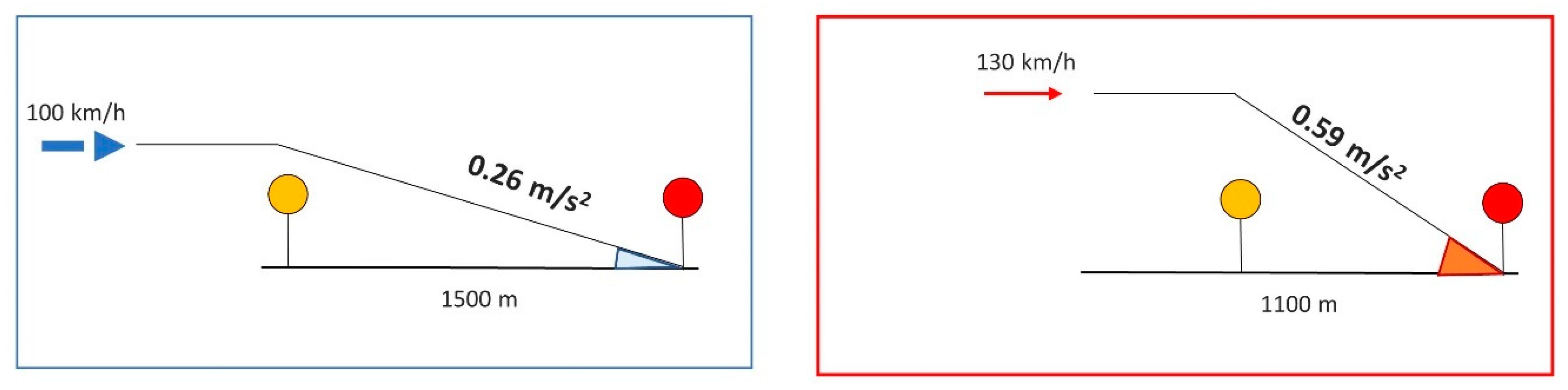
There are multiple forms of variation in rail task design that can cause incorrect schema activation after incidental learning. One type of variation is the combination of variation in permitted track speed and in distance between signals. These cause variation in the amount of deceleration that is necessary to stop in front of the red signal. In Figure 3 it is illustrated that in the left scenario, a continuous deceleration rate of 0.26 m/s² would be sufficient to stop in front of the red signal, while in the situation on the right, a deceleration rate of 0.59 m/s² is needed. If a driver is more often exposed to the situation on the left, then the cue “yellow aspect” can trigger the initiation of a schema resulting in a slower rate of deceleration than required for the situation on the right.

The above example illustrates variation in the required deceleration for the same signal aspect (yellow). In Dutch rail, there is also variation in which signal aspect is present at a given location. Figure 4 shows that signal Sx can have signal aspect yellow:4, as part of a yellow:4 yellow–red sequence. It can also have a yellow aspect as part of a green–yellow–red sequence.

A signal can also have a yellow:number aspect as part of a speed restriction. This kind of speed restriction is sometimes needed to prevent trains from driving too fast over a switch (Figure 5). Aspect yellow:4 indicates a speed restriction to 40 km/h by the next signal, whilst yellow:8 signals a speed restriction to 80 km/h, etc.

In this study, we investigated the effect of the above variations on train driver driving behavior. An additional infrastructure characteristic that was taken into account was the track speed limit just before the first yellow signal. We did not expect to see an effect of incorrect schema activation for those approaches with such low speed that the train driver could start with deceleration upon sight of the red signal and still come to a standstill with mild deceleration. The issue of incorrect schema is assumed to be mostly relevant for those approaches where the train driver needs to decelerate before the red signal is visible. This is because automatic behavior can also occur without the use of schemas. This can occur when the information needed to perform the action is directly available in the environment [21]. When the driver can see the red signal, he can estimate the distance and the best rate of deceleration. When the train driver has to start decelerating before seeing the red signal, he needs to rely fully on the information stored in the schema in his long-term memory.

1.3. Previous Research on Incidental Learning and Task Design Variation

The field of human factors looks at the influence of system or task design on human behavior [22]. There is however a strong focus on task design at the moment of performing the task and not on the potential influence of previous exposure to other task designs. Experience is also mentioned as a positive factor, without the nuance that experience and variation can interact to lead to errors.

Some commonly used taxonomies of human error causes, for example, do not include this factor. One accident analysis method called the Human Factors Analysis and Classification System (HFACS) was inspired by Reasons’ popular Swiss Cheese model and provides a taxonomy of failure across four organizational levels: unsafe acts, preconditions for unsafe acts, unsafe supervision, and organizational influences [23]. Of the seven preconditions for unsafe acts, the “technological environment” is most aligned with the idea of task design. This precondition is further clarified as encompassing “a variety of issues including the design of equipment and controls, display/interface characteristics, checklist layouts, task factors and automation” (p.62). The focus is mostly on the state of the individual at that precise moment, and not the impact of previous learning.

One human reliability analysis method, the SPAR-H method, estimates error probability and contains a list of performance-shaping factors (PSFs). The eight PSFs are: available time, stress/stressor, complexity, experience/training, procedures, ergonomics/human-machine interface, fitness for duty, and work process. The PSF “experience/training” can only be scored as poor, nominal, or good (or it can be considered that there is insufficient information). For this factor, more experience is considered better and reduces the (calculated) probability of an error [24]. In our research, the hypothesis is that greater experience can lead to errors, if combined with problems in task design. The PSF “ergonomics/human-machine interface” comes closest to the idea of task design, but focuses mostly on the state at that moment and not the impact of previous learning.

In scientific SPAD literature, the role of infrastructure elements is mainly considered with respect to visibility and interpretability of the signal [25,26,27]. One study on driver performance modeling and its practical application included line speed as related to signal and sign visibility and reading times [28]. One human factors SPAD hazard checklist contains the following scoring factors: the presence of driver’s personal factors, driver inattentiveness, signal visibility, the association between the signal and the correct line, the ability to read signal aspect correctly, the ability to interpret signal aspect correctly, and the ability to perform correct action [29]. There is no factor for task variation.

Within the rail industry, there are some recommendations on infrastructure variation, such as making sure there is no standard caution or low speed aspect in front of the red signal, because “permanent caution signals, for example, do not provide drivers with information about the next signal, and can therefore be a SPAD trap” [30]. Incident investigations at the Dutch Rail infrastructure manager ProRail have also led to the hypothesis that such locations pose a risk, but the mechanism and the size of the effect are unclear. Up until recently, there was not enough data to test these effects rigorously.

The UK Rail Safety and Standards Board (RSSB) conducted a large-scale investigation in 2016, reviewing 257 industry SPAD investigation reports and organizing SPAD workshops with 60 participants with various job titles from freight operating companies, passenger operating companies, and the UK Infrastructure manager Network Rail [31]. They identified 10 risk management areas, such as signal design/layouts and driver competence management including route knowledge. The recommendations for signal design/layouts focus mostly on visibility of the signal and design of the signal itself and of the gantry. The route knowledge was considered as positive in that report. Route knowledge is also in other countries mentioned as a positive and important factor [32]. Variations in signal aspect shown on the same route are not mentioned.

Balfe, on the other hand, mentions expectation bias as a factor influencing SPADs in her review of 83 internal investigation reports of SPADs occurring between 2005 and 2015 on the Irish rail network [33]. The exact link between expectation bias and infrastructure is not specified. This author does mention the potential for congested networks to result in single or double signals being routinely experienced by drivers across a route, thereby leading to an expectation of continued movement rather than a subsequent stop signal upon seeing a yellow aspect.

1.4. Objective of This Study

The objective of this study was to investigate whether incidental learning impacted employee task performance in the presence of task design variation. We hypothesized that incorrect schema activation caused lower deceleration rates and thereby smaller safety margins between trains and red signals. We focused on similarities in the yellow aspect and the location as triggers for schema activation. The specific question was:

• Does frequent exposure to certain signal aspects (at certain locations) impact the behavior in a (visually) similar but deviating situation?

In previous railway research, research questions like this could not be answered due to small sample size. Thanks to technological developments, we now have different tools that make it possible to answer questions that could not be answered in the past.

1.5. Hypotheses

We hypothesized that incorrect schema activation was a cause of insufficient deceleration, potentially resulting in SPADs or near-misses. We identified four situations where this could occur. The more common signal approach is here referred to as “the standard approach”. The less common approach is referred to as “the deviating approach”. This deviating approach is also the safety-critical approach. If the schema of the standard approach is activated during the deviating approach, then an incorrect schema is activated. The more often the train driver is exposed to the standard situation, the higher the chances of incorrect schema activation during the deviating approach.

In Dutch rail, there are two main types of situations when a specific signal is often yellow and can become “the standard approach”. One situation is when the scheduling is such that the signal at the train’s stopping location is often red. The signal(s) preceding it will be yellow at an equal frequency. We call this “yellow entrance to the station”.

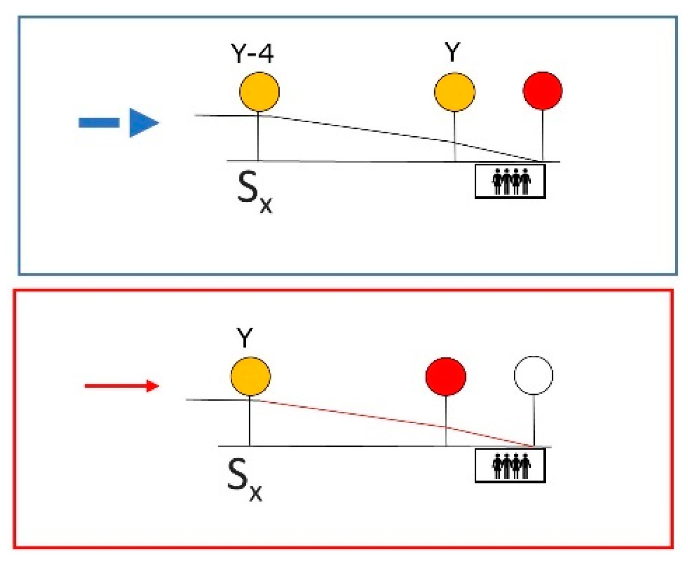
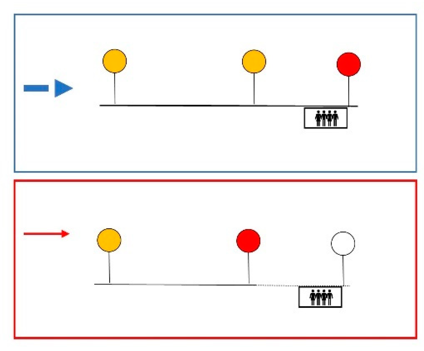
When “yellow entrance” is common, this is the standard situation. The deviating situation is then when one signal earlier is red. In these situations, we can find similarities between the standard and deviating situation in terms of signal aspect and signal location. The required behavior is however different, because an earlier signal is red. In Figure 6, the standard, more common situation is visualized at the top (blue). Below this is the deviating situation (red). In this scenario, the signal aspect and location are exactly the same during both approaches.

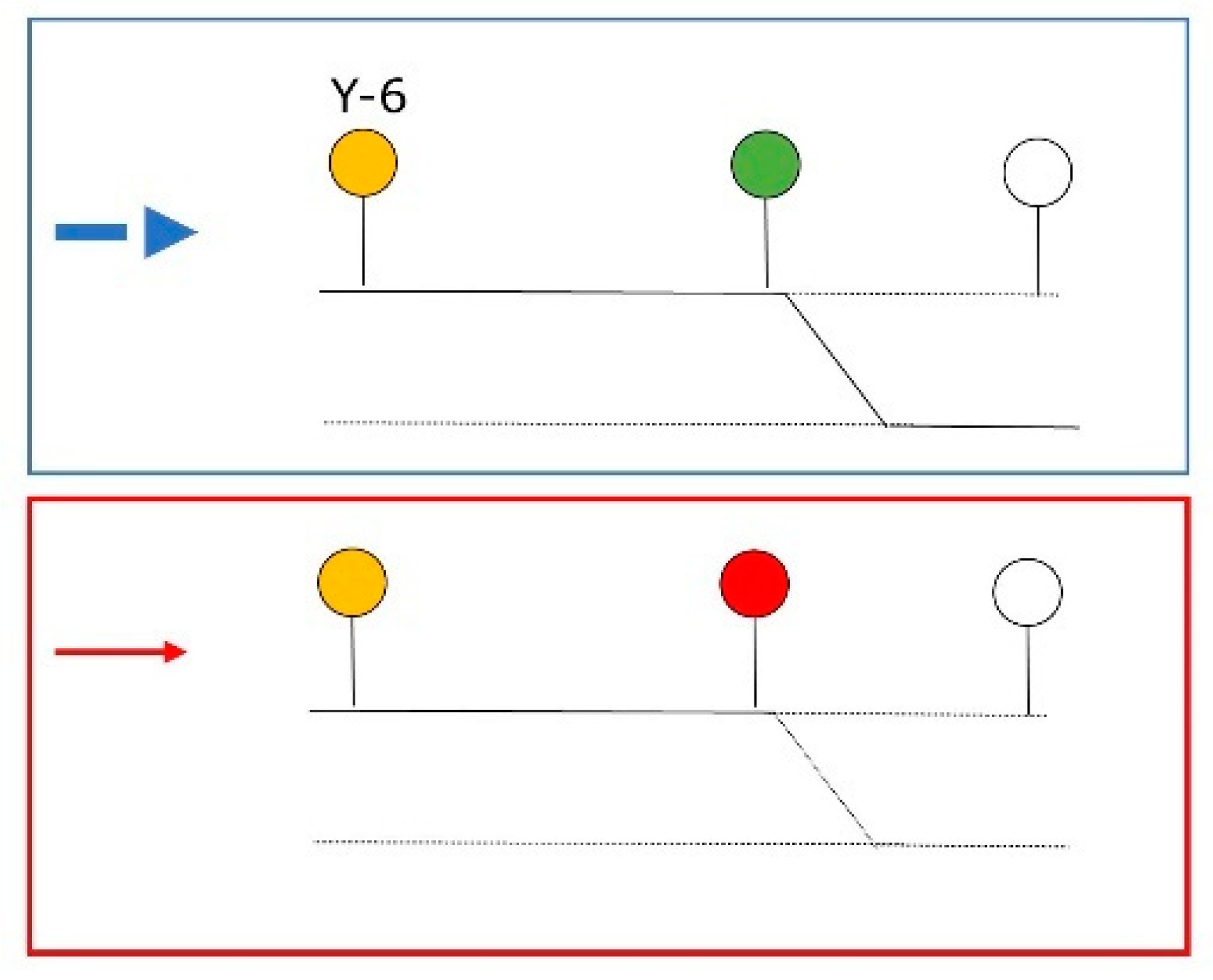
The second main situation where a specific signal is often yellow is when that signal often functions as a speed limit indicator in front of a switch (Figure 7). The standard, more common situation is shown at the top (blue). Below this is the deviating situation (red). In this scenario, the location is exactly the same during both approaches and the signal aspect is visually similar.

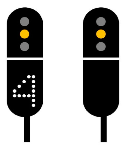
In the above example, the yellow and yellow:number signal aspects are said to be visually similar. Visual similarity is defined by the number of shared points or common features, and the type of difference. Visual similarity is higher with deletion at end points (such as the number 4 missing below) than for differences like deletions leading to breaks in continuity or mirror image reversals [34]. The signals with yellow and yellow:number aspects are thus visually similar because they have many visually identical points with the difference being a deletion at the bottom (Figure 8).

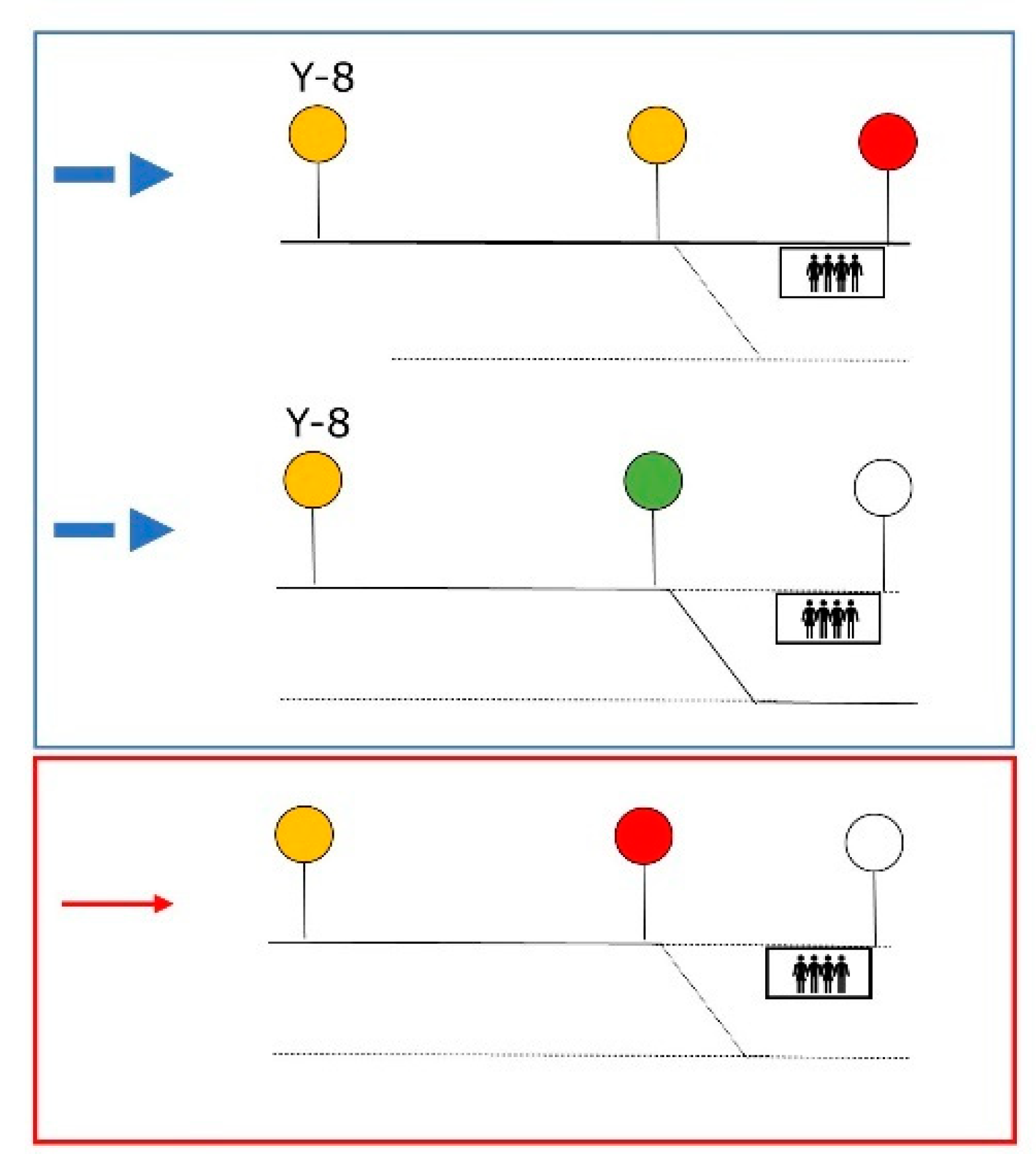
Speed restriction and entrance at yellow can also occur at the same location (Figure 9). While the signal aspects can differ (e.g., yellow:8 and yellow:4), the only relevant situations are those where both are the same.

The last hypothesis encompasses the same signal, but with differences in location. As mentioned previously, the distances between signals varies during approaches where the red aspect is preceded by a yellow and green signal (GR–Y–R approaches). The track speed and signal distance determine the amount of deceleration that is needed. We call this “mean deceleration”. The mean deceleration is not a fixed value. The hypothesis is that GR–Y–R approaches with higher mean deceleration values are deviating situations in comparison to GR–Y–R approaches with lower mean deceleration values (See Figure 10). If the schema of the blue (left) situation is activated during the red (right) situation, insufficient deceleration is used.

2. Method

2.1. The Braking Behavior Measure (Dependent Variable)

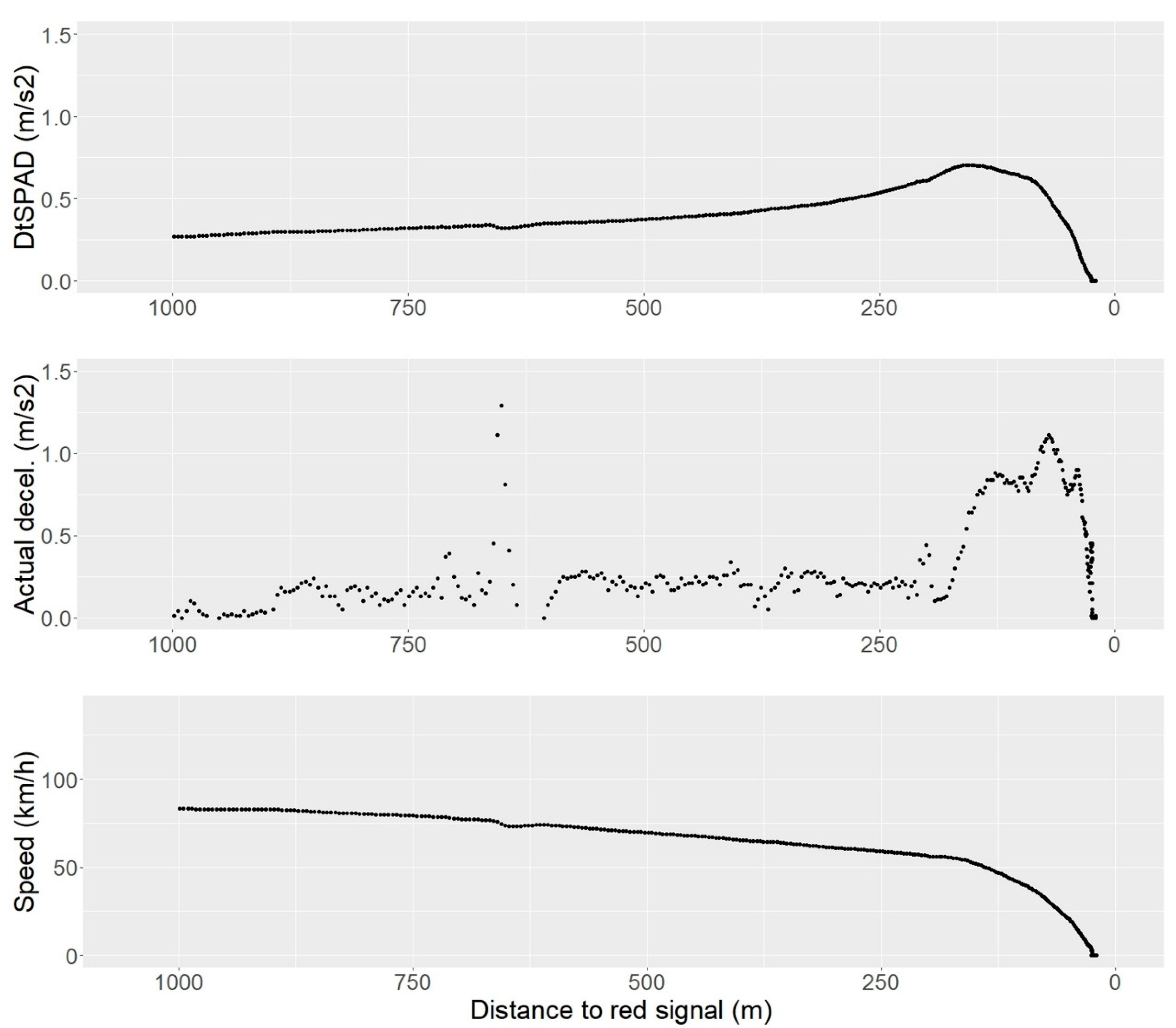
The driving behavior is operationalized in one value for each red aspect approach. The measure is called the maximum deceleration to SPAD (mDtSPAD). First, the deceleration to SPAD is calculated for each location log via the formula DtSPAD = 0.5 $\times$ $spee{d}^2$/distance to red aspect, where speed is measured in meters per second and distance in meters. The DtSPAD indicates the deceleration rate the train needs to maintain to be able to stop exactly at the red signal. The maximum value of these is the mDtSPAD. In Figure 11 the relationship between DtSPAD and actual deceleration is visible. The DtSPAD increases during an approach if the actual deceleration is lower than the DtSPAD value, and the DtSPAD decreases again if the actual deceleration is higher than the DtSPAD value.

The train’s speed and position is needed to calculate the mDtSPAD. This information was gathered from Dutch Railways (NS) trains that have Orbit. Orbit is an auditory SPAD warning system. For this system to work, both the train’s speed and position are registered, among other data. This data is logged multiple times per second from the moment the train is within 1000 m of a red aspect. Frequent logging (more than once per second) made this data source the most suitable. Automatic signals, which cannot be influenced by traffic controllers, are not monitored by the Orbit system due to technical limitations.

In our study we were interested in changes in behavior leading to higher mDtSPAD values. There is no absolute criterion for what constitutes a high DtSPAD value. In this study, 0.5 m/s² was chosen as a criterion for two reasons:

1.

In previous initial analyses with similar data, the mDtSPAD followed a roughly normal distribution. The value of 0.5 m/s² was in the right tail of that distribution.

2.

The Orbit warning system can alter the behavior of the train driver, and thus its mDtSPAD value, if the SPAD alarm sounds. For approaches where the Orbit alarm sounded, the mDtSPAD might have been higher if no warning system had been in place. In previous research it was noted that during most of the relevant approaches the alarm did not sound for DtSPAD values below 0.5 m/s². Unfortunately, the warning does not sound at a specific DtSPAD value. The algorithm for the warning system is based on other indicators that are not suitable for the current study.

Nineteen months of train data were analyzed, starting from 20 August 2018. On this date, approximately 50% of the trains of the operator NS had been equipped with Orbit (±300 trains). More trains were equipped with Orbit following this date, and their data were included as well. All were passenger trains with a brake power of up to 1.0 to 1.4 m/s². Train drivers were from the Dutch operator NS. The NS employs over 3000 train drivers and has 28 places of employment where train drivers start and end their shifts [35,36].

The Orbit system employs a quality filter to the GPS data. The warning system is temporarily shut down when the GPS quality becomes too low. In this study, we only used the data when the warning system was active. We also only included approaches where the time between two logs was always below three seconds.

2.2. Inclusion Criteria

Braking behavior was calculated for the approaches falling within the hypothesis criteria and when:

• For speed: The track speed was higher than 80 km/h according to permanent traffic signs.
• For speed: The train did not pass a yellow signal before the red signal approach as part of a previous red aspect approach. Previous yellow aspects would have already resulted in lower train speed.
• For speed: The train was driving before passing the yellow signal instead of departing from a station.
• For exposure: The red signal remained red until standstill of the train or until the train was within 123 m of the red signal. At 123 m, the train can still have a high value on our risk indicator at a speed of 40 km/h. This is the speed train drivers are instructed to decelerate to after having passed a yellow aspect to be able to stop for the red aspect.
• For other factors: The red signal was not at a scheduled stop location. These approaches were excluded because the train driver would need to stop at these locations regardless of the aspect color.
• For other factors: The speed at which mDtSPAD was recorded was higher than 10 km/h.

2.3. Measures of Variation (Independent Variables)

The two independent variables were the mean deceleration and the frequency of yellow in last 14 days for this train series. The mean deceleration (m/s²) was calculated via 0.5 $\times$ track speed (m/s)²/distance between signals (m). The frequency was calculated by counting the number of times the same train series passed the yellow(-number) signal in the last 14 days. Data from the Dutch infrastructure manager ProRail were used to calculate the frequency so that all train approaches could be used, not just those of trains with Orbit.

2.4. Tests Overview

An approach can be influenced by different effects. To deal with this overlap, the following tests were performed:

• To test the mean deceleration effect, approaches were selected where only the mean deceleration was a factor (exclusion of yellow entrance or yellow speed restriction; n = 3478 red aspect approaches).
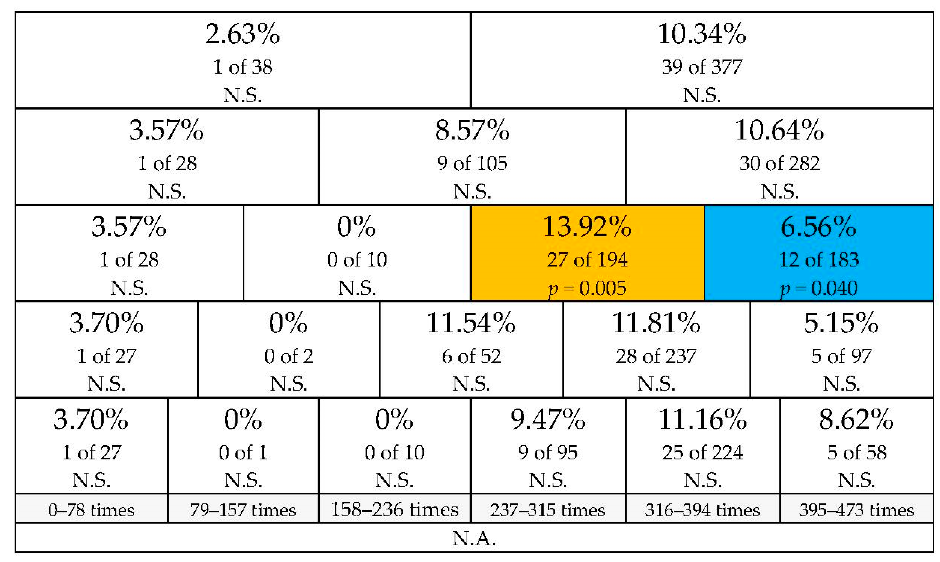
• To test the yellow:number entrance effect, locations with speed restrictions were included if these speed restrictions had the same signal aspect. Three types of tests were done. The first used all the approaches (n = 3429 red aspect approaches). The second used approaches within a specific mean deceleration range (n = 2021 red aspect approaches for a high mean deceleration range and n = 1287 for a low mean deceleration range). The third used approaches towards one specific signal. Only one signal was eligible as it had a sufficiently large number of approaches across different frequencies of entrance at yellow–x (n = 415 red aspect approaches).
• To test the speed restriction effect, approaches were selected where there were speed restrictions via yellow–x and a specific mean deceleration range. Locations with entrance at yellow were excluded (n = 509 red aspect approaches).
• To test the y–y–red effect, all y–y–red locations were included where there was no yellow–x speed restriction or yellow–x station entrance (n = 20 red aspect approaches).

2.5. Statistical Analysis

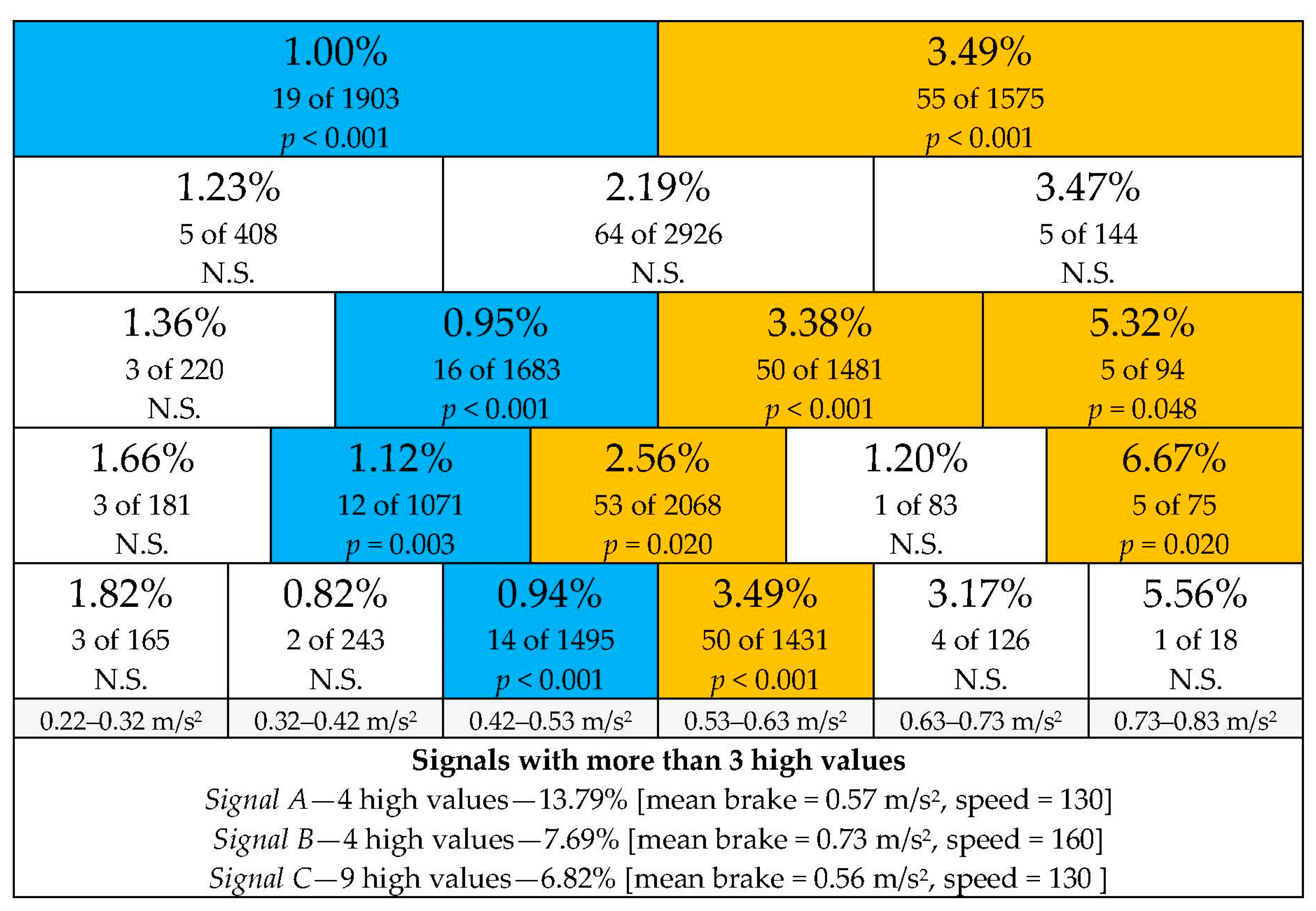
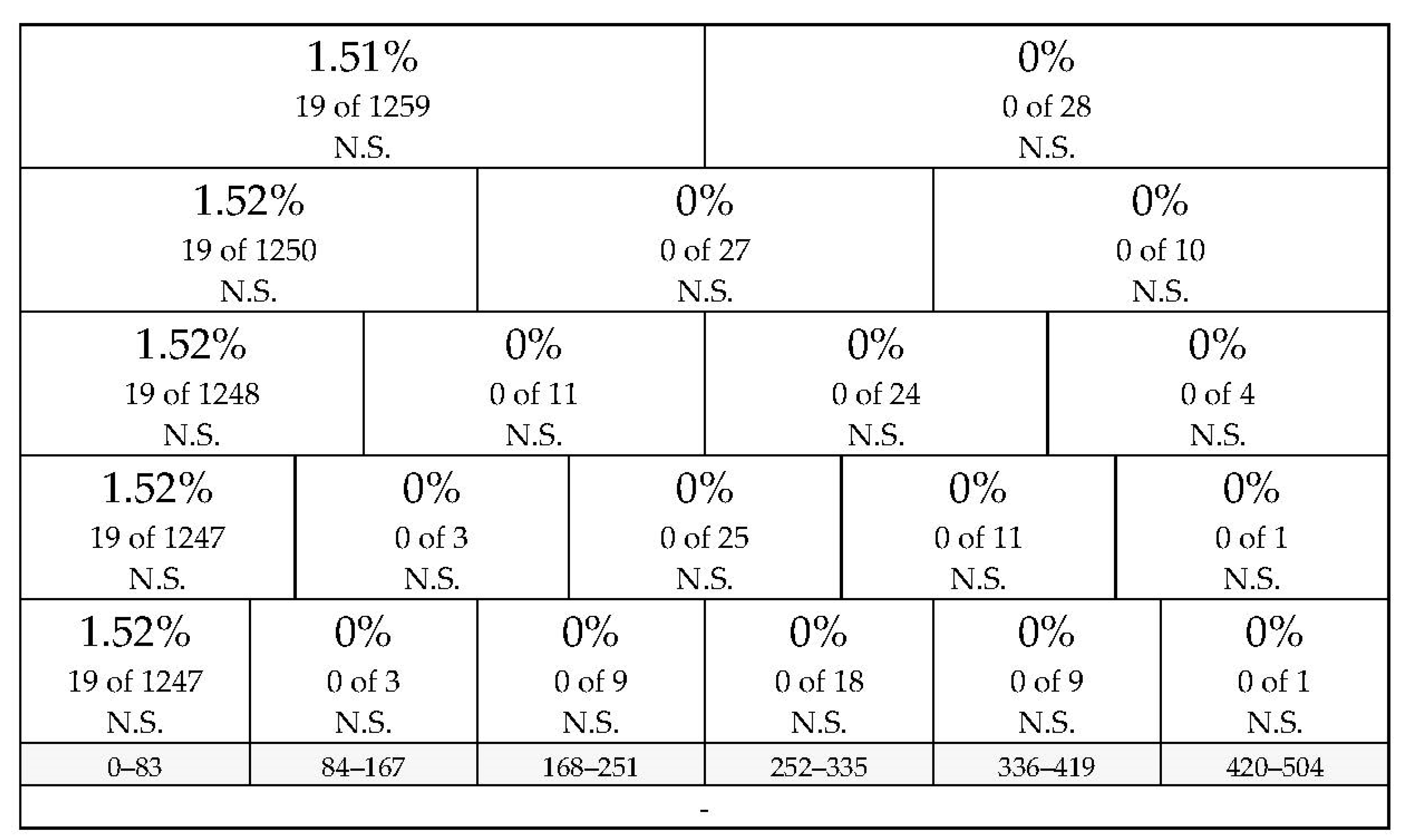
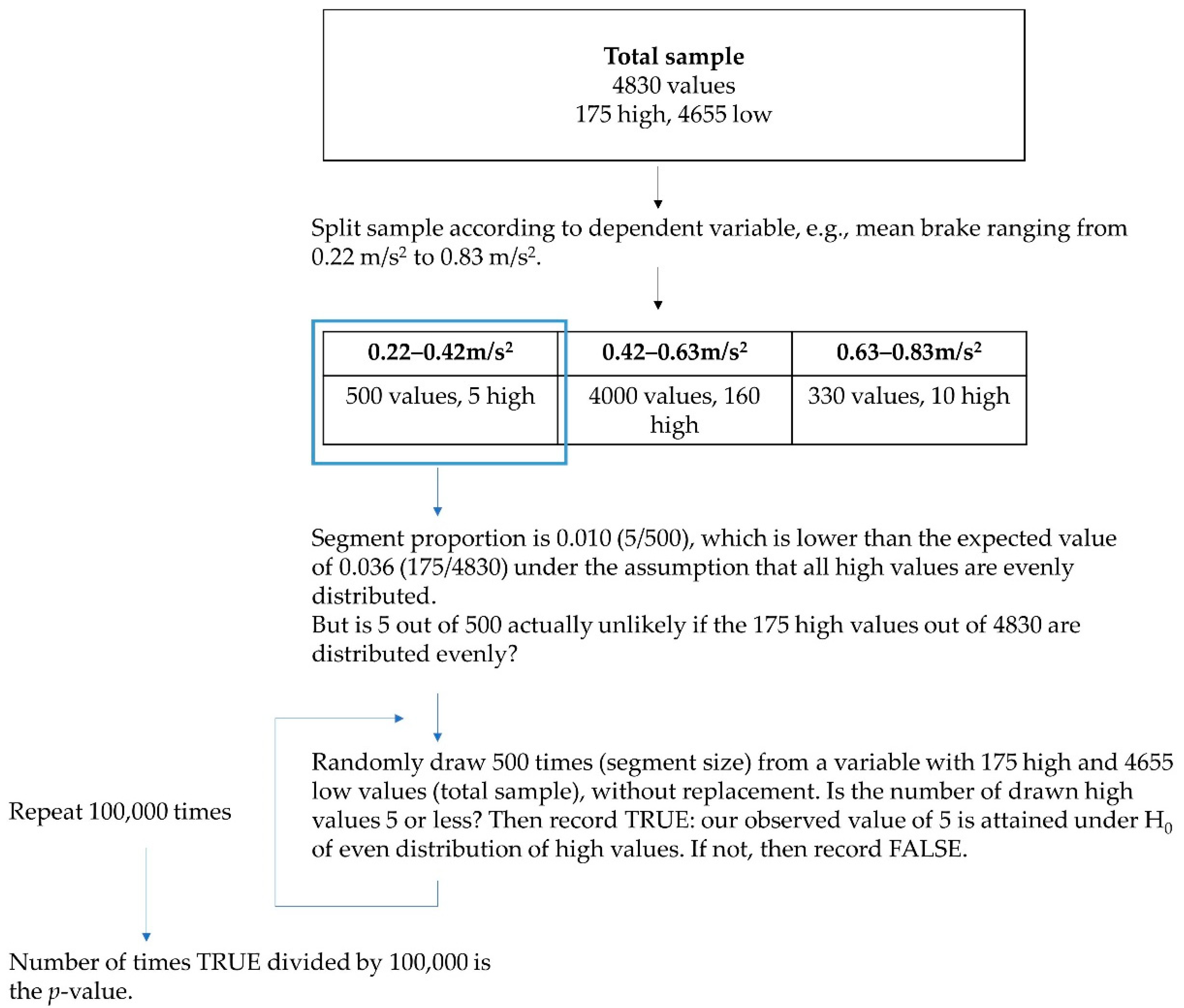
To test the relation between the binary dependent variable and the (ratio) independent variables, a logistic regression analysis was considered. However, the assumption of linearity of independent variables and log odds was violated. Since there was no continuously increasing effect and we wanted to understand the actual shape of the relation, we considered an alternative analysis. In piecewise regression, more than one line is fitted to the data. Multiple points in the independent variable can be chosen to split the data. These points of separation are called knots. Choosing the number of knots and their location is however very difficult. To refrain from using subjective input we decided to split the data evenly five ways. The first split was in half. The second split was in three segments, the third in four segments, the fourth in five segments, and the fifth in six segments. The different splits lead to differences in under- and overfitting and in sample size per segment. Most importantly, insight is provided on the shape of the curve, which can be difficult with a binary dependent variable. The effect of knot selection is also shown. If the pattern remains the same across splits this is evidence for an effect.

The p-value was calculated per segment by comparing the observed number of high values with the number of high values that is expected for the segment under the H0 assumption that there was no difference between segments. The analyses were run in R, version 3.6.2. No additional packages were used for the analyses. The R Code is provided in Appendix A. The steps are clarified with an example in Figure 12.

In the Results section the exact p-values were recorded when they were below 0.05, and were listed as p < 0.001 when they were below 0.001. p-values above 0.05 were recorded as non-significant (N.S.).

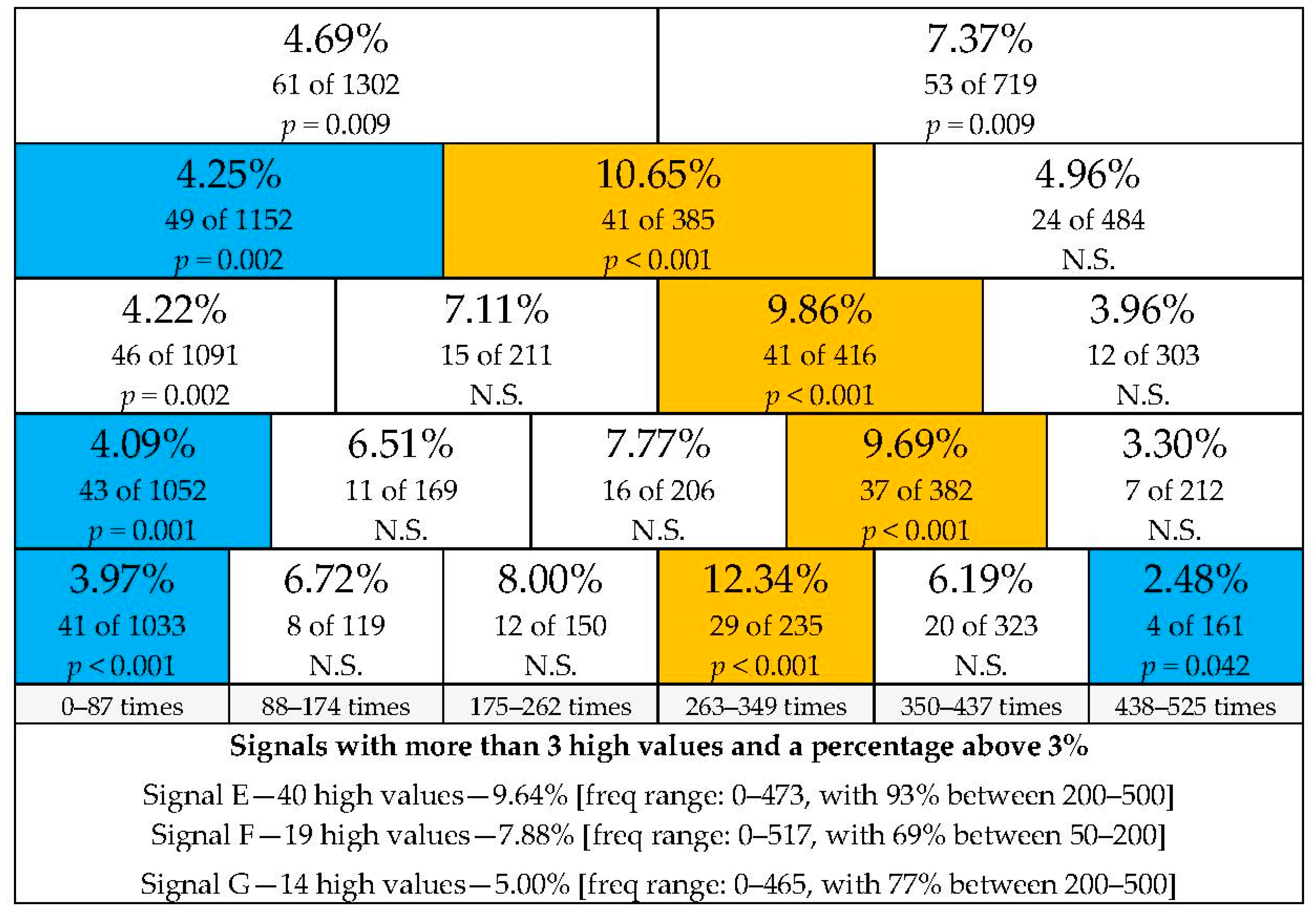
2.6. Signal Effects

It is possible that there are signals which have many approaches with high values. If the results are fully attributable to one or a few signals, the results are less likely to be caused by the investigated variable. To check whether the results were not fully attributable to one or a few signals, signals with more than three high values were identified. These signals are listed in the tables in the Results section and have been used to interpret the results.

3. Results

3.1. Mean Deceleration Effect

If incidental learning occurs, we expect a correlation between the percentage of high values and the mean deceleration, with higher percentages for higher mean decelerations. Figure 13 shows the results with the mean rate on the x-axis. Significant results were found for four out of five splits (i.e., the rows in the figure). In general, the expected pattern was seen, with high percentages for higher mean decelerations (See Figure 13).

Can the effect be caused by an alternative explanation of signal effects?

Signal B is almost solely responsible for the significant cells on the far right, annotated with an asterisk, contributing four out of five high values. This signal had a track speed of 160 km/h. Separate inspection of approaches with track speed of 160 km/h showed that the percentage around a mean deceleration value of 0.6 m/s² seemed lower than those for approaches with track speeds below 160 km/h and a mean deceleration value around 0.6 m/s². It might be the case that approaches at a track speed of 160 km/h are experienced differently. Potentially, (a) this highest mean deceleration segment in fact shows less behavior change and the effect seen is all due to Signal B with other unknown factors; or (b) there is learning within 160 km/h where the mean deceleration value of 0.6 m/s² is experienced as “much space” and only 0.7 m/s² as a “short” distance; or (c) the speed difference is attributable to chance and the effect on the outermost right cells is caused by the mean deceleration effect and not by a signal effect.

The high percentage for the segment between 0.53 and 0.63 m/s² is not attributable to specific signal effects, since there are 50 high values and only 13 of these are caused by two signals that have high percentages.

3.2. Yellow(-Number) Entrance at Station Effect

3.2.1. Yellow Entrance at Station Effect: Analysis 1

The effect of yellow entrance is expected to be higher when the frequency of yellow:number at that location has been higher in the last 14 days, and thereby more learning can have occurred. Figure 14 shows that the significant results follow the expected pattern of increasing percentages. The non-significant outer right percentages are however surprising. Since the total number of approaches is almost 500 for the outer right cell in the second split from the top, this percentage is most likely non-significant because it is close to the mean and is not due low power. The effect on behavior thus seems to taper off, rather than showing the expected continuous increase.

Can the effect be caused by an alternative explanation of signal effects?

A surprisingly high percentage of 22.9% was found for Signal D. Upon inspection by randomly sampling some approaches, it was noted that the preceding yellow signal was often yellow:8 as part of a yellow:8–yellow–red sequence. This red signal was however not at a station stop, which is why these approaches were not added in the calculation of the frequency. Despite the presence of this signal in the outer left segments, these segments are still significant on the lower end. The possible signal effect of Signal D therefore does not affect the interpretation of the pattern.

The other signals have a wide range in frequency which would cause any potential signal effect to be spread out. The signal percentages were not higher than the highest significant cell percentages, making it unlikely that the pattern was fully caused by signal effects.

3.2.2. Yellow Entrance at Station Effect: Analysis 2

The previous analysis contained approaches with different mean decelerations. We know there is a significant effect of mean deceleration. Therefore, the test was repeated using only approaches in the mean deceleration range of 0.5–0.6 m/s². This segment was significant in the mean deceleration analysis (and not potentially explained by a signal effect like the mean deceleration ranges above 0.6 m/s²). The mean deceleration of 0.6 m/s² was the highest mean deceleration value permitted for track speeds up to 140 km/h in the absence of an inclining slope. Signal D was removed from this subset because there seemed to be a frequent yellow:8 aspect at that specific location which was not measured in our current method for frequency calculation (see Section 3.2.1).

Figure 15 shows that the significant results still followed the expected pattern of increasing percentages. There are in fact more significant values, despite a smaller number of approaches. The low percentages on the outer right are surprising. The pattern remains of an effect that tapers off or even has an inverted u-shape.

The prior analysis was repeated for the subset with mean deceleration smaller than 0.5 m/s². None of the splits led to significant cells. There were however relatively few approaches with a high entrance at yellow frequency (See Figure 16). This caused problems with statistical power, especially because the number of approaches was very low in the middle section, which showed the highest percentages in the previous analyses. It is unknown whether there was too little power, or whether the yellow entrance effect was only present in combination with a higher mean deceleration.

3.2.3. Yellow Entrance at Station Effect: Analysis 3

The final analysis for the entrance at yellow effect contains only data from one signal. Figure 17 shows two significant results in the expected direction. Most approaches were concentrated around the frequency of 300, leading to many cells with relatively few total approaches. Although the number of significant cells is underwhelming, the pattern displayed by the percentages is in line with the previous results.

3.3. Speed Restriction Effect

Incidental learning was expected to influence driving behavior in locations where the signal aspect frequently was yellow–number due to speed restrictions. There were 509 approaches at locations with speed restrictions that were not at a yellow station entrance location. Unfortunately, 479 of those had a speed restriction frequency of 0 in the last 14 days. The remaining 30 approaches had a frequency between 1 and 15. There was thus insufficient data to examine this effect separately.

3.4. Yellow–Yellow–Red Effect

There were only 20 approaches that fell within the selection criteria. Many more approaches would have been present if approaches had included where the red aspect was at the station stop during the “deviating approach”. Unfortunately, looking at these planned stops creates many methodological issues, including the influence of the distance between the red signal and the stopping location.

4. Discussion

Can incidental learning contribute to SPAD incidents? In this study we took a step towards answering that question by first checking whether there was evidence of a change in behavior as a result of incidental learning. Significant results were found in the expected direction. Other factors can however also influence the results, like signal effects. Deceleration behavior can be different for certain signals, for example because signal approaches differ in track speed, signal distance, and (early) signal visibility. The “entrance at yellow” effect was however also seen within one specific signal. That result cannot be influenced by any signal effects.

The same result pattern was seen during the other “entrance at yellow” tests. The effect was therefore not only present for the one signal. Unfortunately, there was insufficient data to test whether the effect was also present for signals with a lower mean rate. It is therefore not yet known whether the “entrance at yellow” effect is always present, or only for those approaches with a higher mean rate. It is possible that the approaches with a lower mean rate provide more time for the driver to correct his or her deceleration behavior before it shows up in our behavior measure. In theory, low mean rates might “buffer” against problematic situations. In the Netherlands, the trains are forced to decelerate at a minimal deceleration rate after passing the yellow signal. For approaches with low mean rates in particular this brings the speed down significantly.

The shape of the effect was not entirely as expected for the entrance at yellow effect. The effect seemed to taper off as the entrance at yellow frequency reached very high values. Given the high frequencies, these were approaches where the train series had entrance at yellow almost every time. A potential explanation is that the extreme familiarity with the situation leads to a heightened awareness when something is different. This is comparable to coming to a friend’s house occasionally and going there nearly every day. When visiting occasionally one will recognize the picture on their living room wall. One might not notice when they change the picture to a comparable one. However, when the individual visits nearly every day he/she is more likely to notice that they changed the picture despite minimal changes.

It is of course also possible that there is a hidden factor that happens to be more present for those entrances with the highest frequency of entrance at yellow. This is unlikely, because a similar pattern was seen when looking within one signal, but the possibility cannot be excluded. Further research is needed to see whether the pattern is indeed caused by this psychological effect or whether it was an artefact of our data.

During the “entrance at yellow” effect, incidental learning occurred because the approach was in the same location and with a similar cue (e.g., yellow:4 and yellow). We also obtained evidence of a mean deceleration effect. In these situations, the location is different, but the cue is identical (yellow). The pattern for mean rate was as expected, with higher mean rates leading to higher percentages. However, the high percentages at the highest mean rates were caused by one signal and could thus be the result of a signal effect. Even if this is the case, the pattern remains for the low to medium–high mean rates. It would be jumping to conclusions to say that this pattern was definitely caused by incidental learning. It could be a conscious choice to always decelerate at for example 0.4 m/s², which would lead to a mDtSPAD above 0.5 m/s² for approaches with a mean rate above 0.4 m/s² and to low mDtSPAD values for approaches with a mean rate below 0.4 m/s².

4.1. Limitations and Future Research

In future research, additional factors could be included. One identified factor was the presence of a frequent yellow:number aspect caused by a red signal that was not at a station stop. While the timetable is designed to avoid this kind of approach frequently in the same place, it is of course possible for this to occur. Additional involved factors could be line of sight, with early visibility as a protective factor.

An extra finding was the identification of signals with high percentages. It is clear that there are behavior-influencing factors that are currently out of scope and unknown. Whilst they did not interfere with the conclusions of this research, it would be an interesting avenue to discover what causes these differences between signals.

A limitation of our research was that the exposure frequency was calculated by train series and not by train driver. Since learning takes place in the mind of an individual, it would have been preferable to measure how often the train driver had previously experienced similar situations. Information about the train driver was not disclosed for privacy reasons. The same train series was considered the next best alternative under the assumption that a train driver often drives the same train series. Another possibility was to simply calculate how often any train was exposed to yellow aspects at the relevant location. We however assumed that train drivers link their experiences with the infrastructure to the train series they are in, since their driving experience is influenced by the present train series. A train driver might for example drive from Utrecht to Amsterdam, as many trains do, but the train series he is in determines which stations he has to stop at, what his timetable looks like, and the continuation of his journey.

Fortunately, our research focuses on relative changes. When a train series has an entrance at yellow frequency of 200 over the past 14 days, the specific train driver probably does not experience a yellow entrance in that location all 200 times. However, the train driver is likely to have experienced a greater number of entrances in yellow than in those cases where the frequency was only 100.

Nonetheless, the research would be improved by replication using driver data. This would also give more insight into how often an employee actually needs to be exposed to a certain situation for incidental learning to occur. Another related avenue for future research could be individual differences in incidental learning.

4.2. Answering the Question and Using the Answer

Our results indicate changes in train driver behavior when employees have previously been exposed to different behavior requirements in the same location with a similar yellow signal. The results are in line with our expectations of incidental learning. Using actual data, we identified a shift in braking behavior in the direction of a lower safety margin. We thus found evidence for the notion that incidental learning impacts employee behavior and thereby safety margins.

It is possible that the effects of incidental learning results in SPADs in certain situations. Further research can test whether the effects of incidental learning are indeed also visible using data of actual SPADs. A commonly known disadvantage of using incident data for quantitative analysis is that there is usually a small amount of data since there are relatively few (large) incidents. This is especially the case in the Netherlands when looking at nuanced causes. There are for example multiple SPADs with aspect sequence green–yellow–red, but fewer with that specific aspect sequence and entrance at yellow. There are even fewer incidents within that segment with various frequencies of entrance at yellow. The results of this study, based on data of all red aspect approaches, can be used to focus an analysis with incident data.

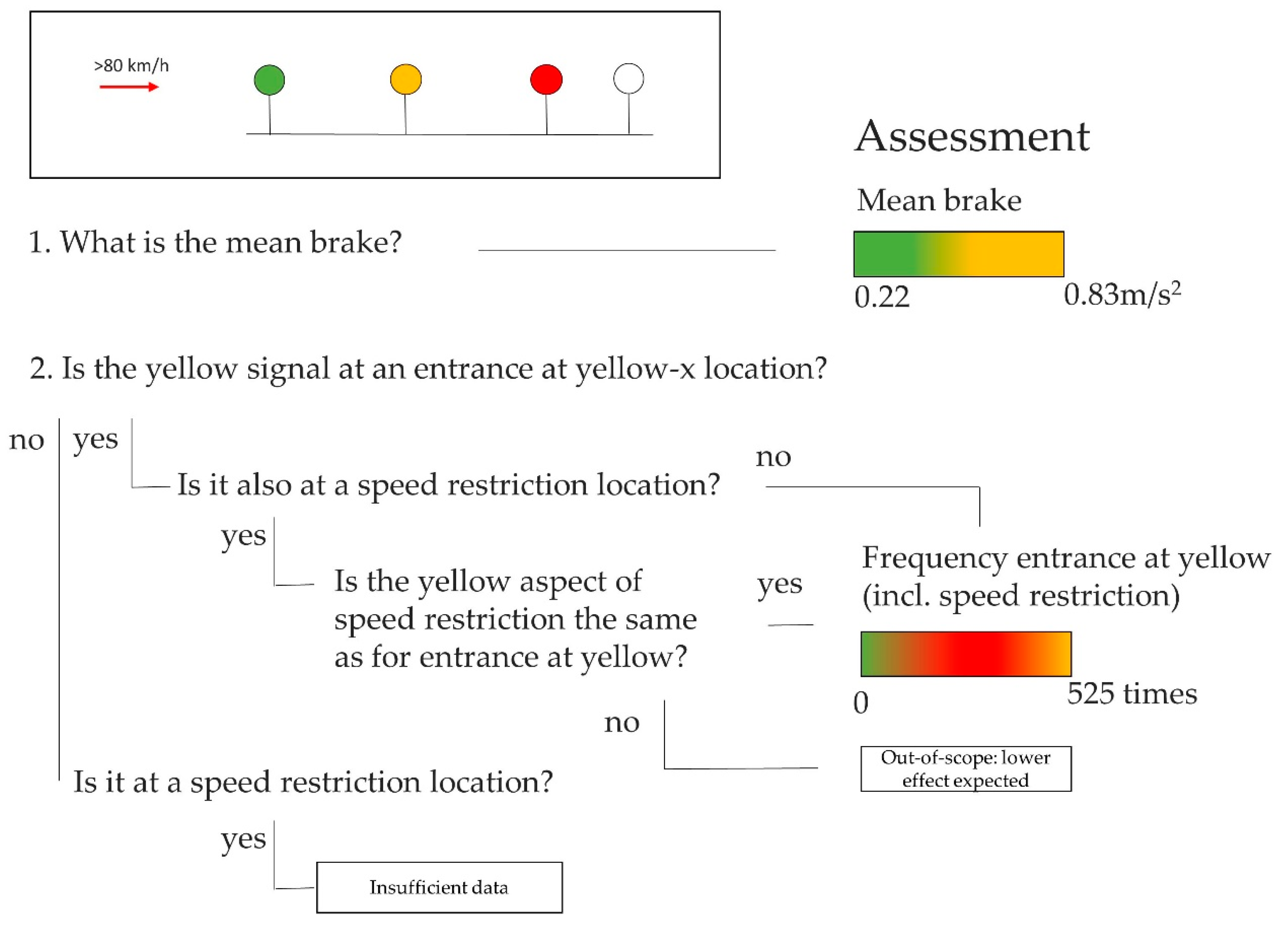
The results of this study can also be used as an input for decision-making on desired interventions. It is clear that crude measures, such as no longer using a specific signal aspect, are not necessary to eliminate certain behaviors or increase safety margins. We see that specific effects add up to create the locations with the highest percentages. Figure 18 gives a simplified overview of how one signal approach can lead to different behavior depending on the mean deceleration, entrance at yellow frequency, and presence of speed restriction.

In a general sense, organizations can reevaluate their task designs by taking the presence of incidental learning into account. Organizations often focus on making sure that the task design for a specific task helps the employee to perform the task successfully. This is important but does not address the whole story. To further improve task design, one should not only consider what the employee is exposed to during the execution of the specific task, but also what he or she has been exposed to during other moments of his shift. Yesterday matters, especially if it is visually similar.