An Examination of the Strava Usage Rate—A Parameter to Estimate Average Annual Daily Bicycle Volumes on Rural Roadways

Abstract

In Spain, a new challenge is emerging due to the increase of many recreational bicyclists on two-lane rural roads. These facilities have been mainly designed for motorized vehicles, so the coexistence of cyclists and drivers produces an impact, in terms of road safety and operation. In order to analyze the occurrence of crashes and enhance safety for bicycling, it is crucial to know the cycling volume. Standard procedures recommend using data from permanent stations and temporary short counts, but bicycle volumes are rarely monitored in rural roads. However, bicyclists tend to track their leisure and exercise activities with fitness apps that use GPS. In this context, this research aims at analyzing the daily and seasonal variability of the Strava Usage Rate (SUR), defined as the proportion of bicyclists using the Strava app along a certain segment on rural highways, to estimate the Annual Average Daily Bicycle (AADB) volume on rural roads. The findings of this study offer possible solutions to policy makers in terms of planning and design of the cycling network. Moreover, the use of crowdsourced data from the Strava app will potentially save costs to public agencies, since public data could replace costly counting campaigns.

1. Introduction

In the European Union, although the number of cyclist deaths has decreased by 27% between 2006 and 2015, cyclist fatalities account for a large percentage (8%) of the total fatalities on road crashes [1]. Over the same period of time, the number of cyclist deaths has raised by 6% in the United States, reaching a total of 818 fatalities in 2015 [2]. Therefore, cycling safety is becoming more and more important in our society.

In 2018, 7598 fatal-and-injury crashes involving bicyclists occurred in Spain, resulting in 58 deaths, 620 serious injuries, and 6633 minor injuries [3]. Although most of these crashes took place on urban areas (74%), 40 of the total number of fatalities occurred on two-lane rural roads, which are used by many recreational bicyclists for leisure and fitness. This type of road accounts for 90% of the Spanish road network, being three times more likely to have fatal-and-injury crashes compared to urban roads.

Road crashes are very connected to risk exposure. Every single interaction among cyclists and/or with motor vehicles increases the likelihood of having a road crash. A motor vehicle overtaking a bicycle has been reported as the most dangerous maneuver due to the higher relative speed difference [4]. There are many other aspects that do influence the safety outcome of a road facility, but an adequate determination of the number of cyclists (“exposure to risk”) is considered by many researchers as the most challenging one [5].

An adequate estimation of risk exposure would allow road agencies and researchers to determine crash rates (i.e., number of crashes per exposure estimator) to compare the risk level across facilities and prioritize actions. A more advanced methodology is through Safety Performance Functions (SPFs) (Equation (1)). A SPF is a function that relates risk exposure and other explanatory variables (e.g., geometric design indexes or the posted speed limit) to the number of road crashes [6,7].

$$y=e^{{\beta }_0}·AAD{T}^{{\beta }_1}·L^{{\beta }_2}·e^{{\displaystyle \sum }{\beta }_i·x_i}$$

(1)

where y is the number of road crashes, AADT is the Annual Average Daily Traffic Volume, L is the length of the road segment, x_i are the explanatory variables, and ${\beta }_i$ are the corresponding regression coefficients.

Although many recent studies focused on calibrating SPFs only considering motorized traffic volumes [8,9,10], the current increase of cycling demand on two-lane rural roads suggests the inclusion of the interaction of both motorized and bicycle traffic to assess road safety in a more accurate way [5].

In this context, the Annual Average Daily Bicycle (AADB) volume is considered one of the most important volume metrics for bicycle traffic [11]. AADB is of great interest for many applications, such as economic evaluation of cycling projects, prioritization of cycling infrastructure investments, and road safety analyses. Furthermore, the spatial distribution of cycling demand, represented by AADB, allows engineers to better plan and design the cycling network.

Nevertheless, there is no technology that can perfectly measure AADB. Existing equipment for continuously counting bicyclists, such as inductive loops, pneumatic tubes, infrared detection, and automated video processing, present errors due to occlusion, i.e., the masking of bicyclists that are traveling in platoons [12]. Additional errors can also arise due to equipment malfunction over prolonged outdoor use that spans 24 h a day for 365 days a year. To overcome these data gaps, El Esawey [11] proposed the use of either count data models (log-linear and negative binomial models) or an autoencoder neural network model, which relate weather-specific and time-specific attributes to the daily cycling demand, instead of historical average methods, which do not incorporate weather effects.

The Traffic Monitoring Guide (TMG), published by the Federal Highway Administration (FHWA) [13], describes current technologies for monitoring nonmotorized traffic, the volume variability of nonmotorized traffic, and proposed data collection programs.

The guide recommends using data from permanent stations and temporary short-count sites to characterize the spatial variability of nonmotorized traffic. Continuous counts are used to classify sites into different groups, in which monthly and daily adjustment factors are calculated. These adjustment factors are then applied to a larger number of short duration counts to estimate the annual average daily traffic of nonmotorized traffic at a network level through Equation (2).

$$AADB=D·F_m·F_d$$

(2)

where D is the short-duration count, F_m is an adjustment factor for the month, and F_d is the day-of-week factor.

The estimation of cycling traffic volumes and the development and application of adjustment factors have been thoroughly studied in recent years [14,15,16,17,18,19,20,21,22]. Additionally, different models currently exist for the estimation of bicycle traffic volumes [11,23,24,25,26,27,28,29]. Although these models differ in terms of their procedures, data needs, and reported accuracy, most of them relate hourly/daily bicycle volumes to either weather conditions or land-use characteristics. The results of these studies are generally consistent, though the magnitude of the impact might vary from one city/country to another. Cycling demand has been found to increase with moderate-warm temperatures (<30 °C). Likewise, the rain and wind induce lower cycling demands.

Besides that, the growth in the number of users of fitness apps, such as Strava, establishes a good opportunity to analyze the potential of these naturalistic data. Strava allows their users to track athletic activity via satellite navigation and upload and share them afterwards. It can be used for several sporting activities, being cycling one of the most popular. Although Strava sells their data in an anonymized and aggregated way, they also provide a portion of their data for free [30].

Cintia et al. [31] analyzed trajectories, average speed, track duration, and heartrate of nearly 30,000 bicyclists to study fitness performance. Clarke and Steele [32] used Strava data to improve transportation design and urban planning, whereas Jónasson et al. [33] studied cycle route choice patterns.

Some researchers have cautioned about the lack of accuracy of Strava and similar data sources that might lead to biased estimates. Goodchild et al. [34] reported user-bias for fitness apps. Watkins et al. [35] also reported bias towards male and younger riders when comparing Strava with another smartphone app called CycleTracks. While Jestico et al. [36] found only moderate relationship between Strava volumes and observed counts, Haworth et al. [37] identified a close relationship between Strava data and those provided by the London Cycle Census. Finally, Hochmair et al. [38] concluded that Strava data can be considered a useful supplement to other bicycle count systems.

However, most of these studies focused on urban areas where, presumably, recreational cycling, especially for fitness and training, is only a small proportion of the total volume. On rural highways, the majority of bicycling is most likely for recreational purposes and exhibits different characteristics, such as time of day, trip length, bicyclist demographics, and Strava usage. Regarding this, García et al. [39] defined the Strava Usage Rate (SUR) as the proportion of bicyclists using Strava along a certain road segment. The pilot study showed that the SUR was around 25% on this type of roads. Likewise, López-Maldonado et al. [40] collected bicycle volumes in three different rural areas in the Province of Valencia (Spain). These data, which resulted in 27,000 observed bicyclists, were compared with Strava data for each day of observation. In this case, the SUR ranged from 15% to 30%. This was considered as a too wide range, so further research was recommended to explore the reasons behind.

This study goes a step further in the analysis of the evolution of the Strava Usage Rate (SUR), looking at its temporal variability, and proposing a methodology for its calibration. As stated before, the use of apps like Strava is highly correlated to amateur-professional users. Therefore, higher SUR parameters might be linked to more demanding routes. Like in previous research, SUR will be estimated by comparing the observed bicyclists with the uploaded tracks to Strava database. Confidence intervals for the SUR parameter will be given, based on the bicycle hourly volume. This provides a first reliability measure of this factor which will allow the estimation of the Annual Average Daily Bicycle (AADB) volume on two-lane rural roads.

In this way, the paper is structured in four main sections. Section 2 has been divided into two subsections. Section 2.1 describes the methodology, including the SUR definition and how confidence intervals and its robustness are determined. Section 2.2 includes the data collection campaign: field data collection and the Strava data download. Afterwards, Section 3 shows the results for the SUR parameter and its variability. Section 3.1 explores its regional variability, while Section 3.3 analyzes the hourly variation using the sliding window method. To do so, Section 3.2 is first introduced to explore the different sliding window options. In Section 4, a new methodology to estimate AADB is presented and the application of this estimation is discussed. Finally, Section 5 includes the main conclusions of the research.

2. Methods and Data Description

This section is divided into two subsections. In the first one (Methodology), the SUR concept is introduced. Information to determine its robustness, by means of confidence intervals, is also provided. The second subsection (data collection) comprises the different observation points that have been selected for the study, as well as the two data collection campaigns: one in field and another one downloading data from the Strava platform.

2.1. Methodology

The SUR rate can be obtained for a single road facility by dividing the amount of Strava tracks uploaded to the platform by the observed cyclists (Equation (3)), for a certain period of time.

$$SUR=\frac{V_{Str}}{V_{obs}}$$

(3)

where $V_{Str}$ is the amount of Strava tracks and $V_{obs}$ is the number of observed bicyclists. Both volumes correspond to the same time period.

Like for traffic volume estimation, observed and Strava counts must be considered aggregated in periods of time (e.g., 5, 15, or 60 min). This integration is performed through the sliding window methodology, which can also be used to determine the daily SUR or SUR variations within a day.

However, it is important to highlight that any SUR determination following Equation (3) will provide an observed Strava Usage Rate, i.e., the instantaneous or time-aggregated rate. This rate might vary, but a hypothesis of this research is that a certain SUR value exists and can be calibrated for any location. To this regard, the SUR might present regional, seasonal, or hourly variations.

2.1.1. Confidence Intervals

Let us assume that the probability of a cyclist to upload their track to Strava is known for a given location and time ($\overline{SUR}$). Let us also assume that this probability remains the same for all cyclists that ride throughout that position at that time. Thus, for this specific position and time, the probability of having $x$ cyclists tracking their session with Strava in a global count of $n$ cyclists, follows a Binomial Distribution. This probability can be calculated with Equation (4).

$$P\left(B\left(n,\overline{SUR}\right)=x\right)=\left(\begin{array}{c}n\\ x\end{array}\right)·{\overline{SUR}}^x·{\left(1-\overline{SUR}\right)}^{n-x}$$

(4)

As an example, in a global count of 120 cyclists, assuming $\overline{SUR}=0.25$, the probability of 36 of them using Strava is 0.03676.

However, the actual value of $\overline{SUR}$ is unknown. With observation and Strava tracks we can only estimate $SUR$ as $x/n$. Nevertheless, this value can be used to get the confidence intervals for $\overline{SUR}$. Since the binomial distribution is discrete, the cumulative probability function must be calculated prior to any confidence interval determination (Equation (5)).

$$P\left(B\left(n,\overline{SUR}\right)\le x\right)={\displaystyle \sum }_{m=0}^{x}P\left(B\left(n,\overline{SUR}\right)=m\right)={\displaystyle \sum }_{m=0}^x\left(\begin{array}{c}n\\ m\end{array}\right)·{\overline{SUR}}^m·{\left(1-\overline{SUR}\right)}^{n-m}$$

(5)

Equations (6) and (7), which are based on Equation (5), allow the calculation of an interval for the expected cyclists using Strava (x).

$$x_l\in \mathbb{N} | {\displaystyle \sum }_{m=0}^{x_l}\left(\begin{array}{c}n\\ m\end{array}\right)·{\overline{SUR}}^m·{\left(1-\overline{SUR}\right)}^{n-m}\cong \frac{1-Z}{2}$$

(6)

$$x_u\in \mathbb{N} | {\displaystyle \sum }_{m=0}^{x_u}\left(\begin{array}{c}n\\ m\end{array}\right)·{\overline{SUR}}^m·{\left(1-\overline{SUR}\right)}^{n-m}\cong 1-\frac{1-Z}{2}$$

(7)

where $x_l$ and $x_u$ are the lower and upper bounds of this interval and must be integer. $Z$ is the confidence value, normally assumed as 0.95.

Note that since these boundaries are discrete, it is impossible to equal the final term. In addition, we are entering in these equations with the $\overline{SUR}$ parameter, which still remains unknown. However, we can rearrange these expressions to obtain the confidence intervals for any observed $SUR=x/n$ (Equations (8) and (9)).

$$\overline{SU{R}_l}\in ℝ | {\displaystyle \sum }_{m=0}^x\left(\begin{array}{c}n\\ m\end{array}\right)·{\overline{SU{R}_l}}^m·{\left(1-\overline{SU{R}_{-}}\right)}^{n-m}=1-\frac{1-Z}{2}$$

(8)

$$\overline{SU{R}_u}\in ℝ | {\displaystyle \sum }_{m=0}^x\left(\begin{array}{c}n\\ m\end{array}\right)·{\overline{SU{R}_u}}^m·{\left(1-\overline{SU{R}_{+}}\right)}^{n-m}=\frac{1-Z}{2}$$

(9)

where $\overline{SU{R}_l}$ and $\overline{SU{R}_u}$ are the lower and upper confidence intervals for a given number of observed cyclists ($n$) and a given number of Strava tracks ($x$). $Z$ is the confidence level (0.95 is proposed). Note that $\overline{SUR}$ is a continuous, decimal parameter, so these confidence intervals equal the final term.

This calculation can be done for any period of time, either a sliding window, a whole day/week, or even a year. As a result, not only can we manage the measured $SUR$ value but also the range within the actual $\overline{SUR}$ that is expected. This range will vary in magnitude and amplitude along the day and date, which will be explored in the Results section.

2.1.2. SUR Robustness

The SUR factor has been proven to be unstable, presenting variations that need to be explored. Thus, it is necessary to perform adequate calibrations to estimate AADB.

SUR stability can be defined as how reliable a certain SUR factor is, according to its calibration conditions. Regarding this, an important question arises: how should a SUR factor be calibrated to be reliable?

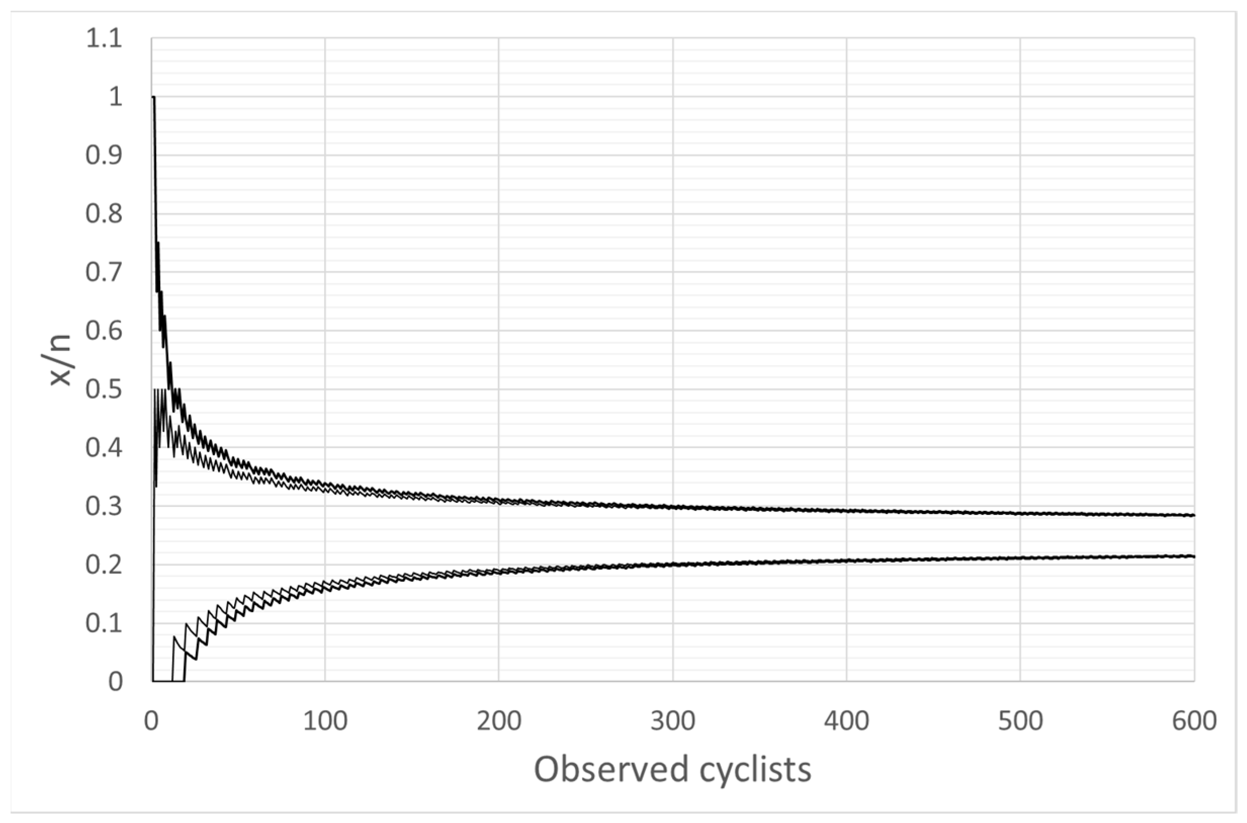
Calibration conditions could be set as a function of observed cyclists or observation time. As previously mentioned, the binomial distribution controls the likelihood of $x$ cyclists tracking their activities, from $n$ observed cyclists, given a certain $\overline{SUR}$. Figure 1 shows the sampling likelihood distribution for $\overline{SUR}=0.25$, i.e., the likely sample SUR that we can determine at a 95% confidence level, given a global $\overline{SUR}=0.25$.

For low number of cyclists (e.g., 100 cyclists), the SUR determination becomes very weak. Field SUR direct estimations might even result in 0.12 to 0.36, or even more.

On the other hand, the SUR estimation becomes much more robust as the number of observed cyclists increases. For instance, for 200 cyclists the SUR does not differ more than 0.05 from the actual SUR value, which is a very good approach.

It is important to highlight the relationship between the SUR and existing cycling demand on the road. Some roads have very a reduced demand, thus preventing us from getting an accurate SUR parameter. However, a lower demand makes these roads less important for AADB estimation.

2.2. Data Collection

In order to see how the SUR parameter performs, three important cycling zones have been selected. Data will be obtained at those zones, both from the Strava app and in field, for the same time periods. These zones were located in Valencia (Spain) and were identified as: (i) “El Saler”; (ii) “Bétera”; and (iii) “Montserrat” (Figure 2)

• “El Saler” area is in southern Valencia. This zone is quite close to Valencia city and presents level terrain due to its proximity to the seacoast. Both the nondemanding longitudinal profile and the touristic attraction of the area make this zone highly demanded for nonprofessional cyclists. Professional ones also frequent this zone, since it serves as a connection to other areas.
• On the contrary, “Bétera” area is a hilly route located to the northwest of Valencia, so it contains significant longitudinal grades. As a result, more professional cyclists are expected in this area.
• Finally, “Montserrat” area lies in southwest Valencia, requiring a moderate physical effort. While it presents a lower physical demand, its higher distance to the main city reduces its potential demand or makes that only most professional cyclists can visit the zone from the city.

Despite the overall variations in longitudinal grade, there are also important differences in cross-section, pavement conditions, and further connections to other regions. These variations might also influence the SUR.

Therefore, it is necessary to perform an in-depth examination of the SUR variation within every zone. A set of different observation points (OP) were strategically located at roads with different cross-sections, longitudinal grades, and pavement conditions (see Figure 2). The only requirement was the estimated bicycle volume to be non-negligible, since the scope of the research is to provide accurate bicycle volume estimation for high-demanded roads.

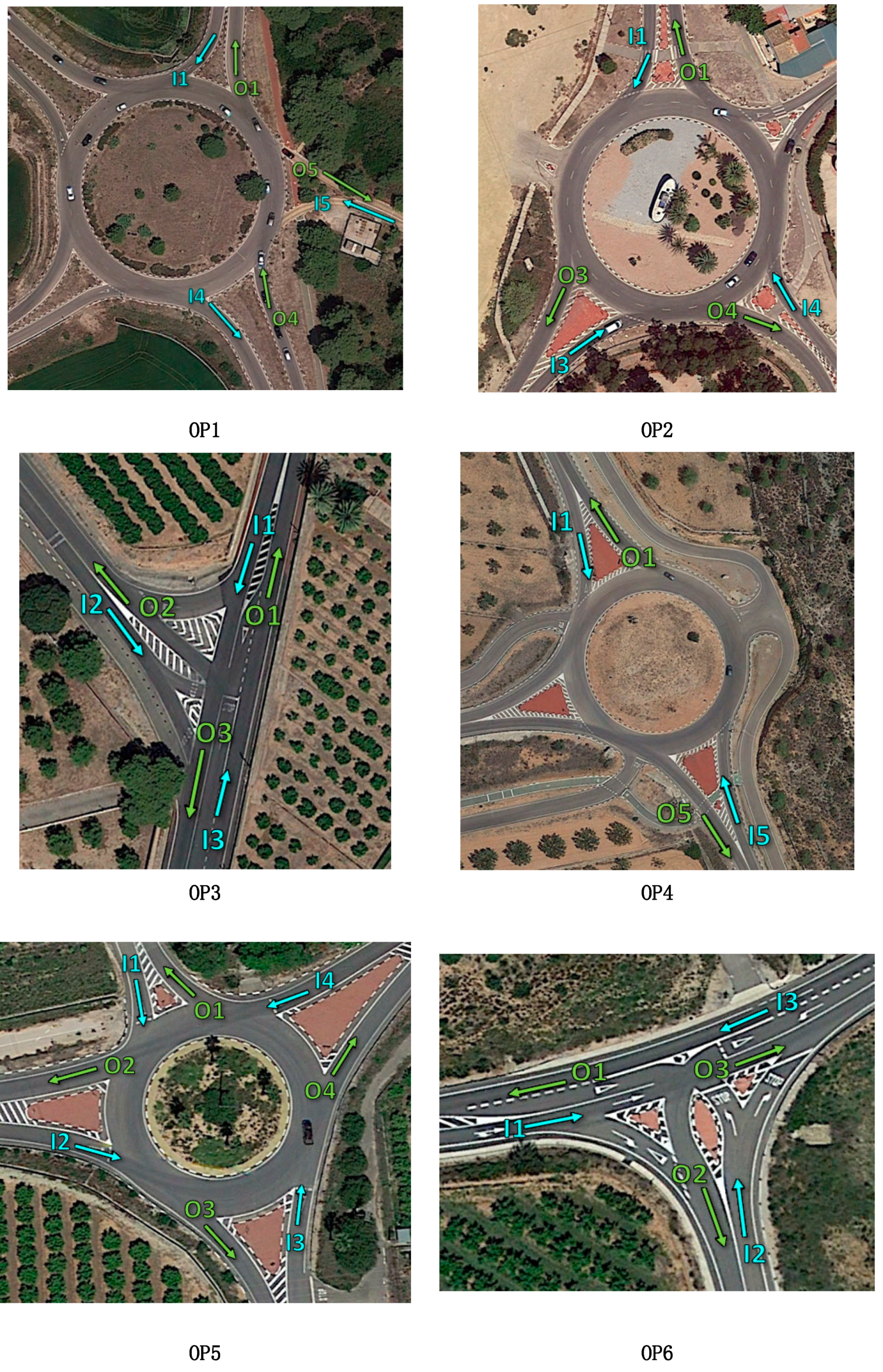
Since the bicycle volume remains constant along a single road segment, road intersections allowed the control of at least three different road segments, hence being an appropriate location for the observation points. Six observation points were proposed, two per study area, allowing the observation of 16 road segments (32 directions in total). Figure 3 presents the aerial view of all observation points and road segments.

OP1 is a roundabout close to Valencia city (which is located at north, connected to In1/Off1 (noted I1/O1 in Figure 3). Road segments I1, O1, I4, and O4 present similar characteristics, being the only difference that the bike lane adjacent to I4 and O4 stops abruptly a few hectometers southwards. As a result, more professional cyclists are expected in I4 and O4.

OP2 corresponds to the same road, several kilometers southwards, further from Valencia city. Although also being in level terrain, cycling demand is quite lower, so higher SUR variability is expected. The most common route included I1/O1 (connecting to Valencia) and I4/O4.

OP3 is a T intersection with high traffic volumes of cyclists and motor vehicles. This is a major junction, providing connection to many important roads.

OP4 is located northwest several kilometers away. This is a roundabout connecting two important roads, all of them with separated bike lanes. Traffic volume is quite low in this roundabout, so less professional cyclists are expected. In addition, being further away from Valencia induces a lower overall demand.

OP5 and OP6 correspond to a roundabout and a T intersection that connect four and three roads, respectively. Both are located in a mountainous area at western Valencia, far away to identify any clear route pattern.

2.2.1. Field Study

All data collections were carried out under favorable weather conditions between April and October 2017. While a data collection along the entire year and considering more days would have been desirable to capture the seasonal variability of SUR, it was not possible due to budgetary constraints. Therefore, the data collection campaigns focused where the highest cycling demand was expected (weekday and weekend mornings). Some afternoon data collections were also performed, to get insight about the SUR performance.

Table 1. Field data collection.

Strategic Location	Observation Code *	Date ** (mm/dd/yy)	Day of Week	Start Time	Finish Time	Observed Cyclists	Cyclists Using Strava
OP1	1.1	05/17/17	W	7:15	11:00	201	47
	1.2	05/17/17	W	15:00	17:00	81	25
	1.3	07/20/17	Th	7:00	10:30	242	56
	1.4	07/23/17	Su	7:45	11:30	465	82
	1.5	09/28/17	Th	8:00	12:30	599	89
	1.6	10/28/17	Sa	8:25	12:15	945	233
OP2	2.1	05/17/17	W	15:00	17:00	174	30
	2.2	05/17/17	W	7:15	11:00	41	25
	2.3	07/20/17	Th	7:00	10:30	260	29
	2.4	07/23/17	Su	8:00	11:20	536	115
	2.5	09/28/17	Th	10:20	11:55	242	40
	2.6	10/28/17	Sa	8:45	11:50	792	215
OP3	3.1	04/05/17	Th	8:00	12:00	206	53
	3.2	04/05/17	Th	15:00	16:15	58	32
	3.3	06/27/17	Tu	7:00	12:00	555	145
	3.4	07/09/17	Su	7:00	10:45	960	276
OP4	4.1	04/05/17	Th	8:00	11:45	82	17
	4.2	04/05/17	Th	15:00	16:30	26	12
	4.3	06/27/17	Tu	7:45	11:30	304	66
	4.4	07/09/17	Su	7:15	10:15	594	168
OP5	5.1	06/03/17	Sa	7:30	12:15	345	102
	5.2	08/01/17	Tu	7:00	11:30	186	29
	5.3	10/19/17	Th	8:00	12:35	115	25
OP6	6.1	06/03/17	Sa	9:00	12:00	164	50
	6.2	08/01/17	Tu	7:30	11:00	101	27
	6.3	10/19/17	Th	8:45	12:00	68	25
					TOTAL	8141	2013

* Observation code is used as unique identifier instead of date because some days present two data collections. ** nonworking day in bold.

summarizes the field data collection.

2.2.2. Strava Data

Strava data were obtained from the Strava segment database, which contains the travel times of everyone who has ever covered a specific segment. The number of cyclists and their timestamp were obtained through an ArcGIS tool developed by the Highway Engineering Research Group using modifiable Python programming code based on the Strava API [39]. This tool allows downloading specific information of the cyclists who had passed through a Strava segment during a certain period of time. The most remarkable information of the downloaded data was the timestamp associated with each cyclist, which was used for the analysis.

3. Results

In this section, the SUR results are presented. First, the outcomes for each observation process are shown. Some interpretation about the variability in volumes and SUR thresholds are provided. Afterwards, the hourly and regional variation of SUR are explored. To do so, the aggregation time period has to be determined first, through the sliding window method.

3.1. Variability across Observation Points

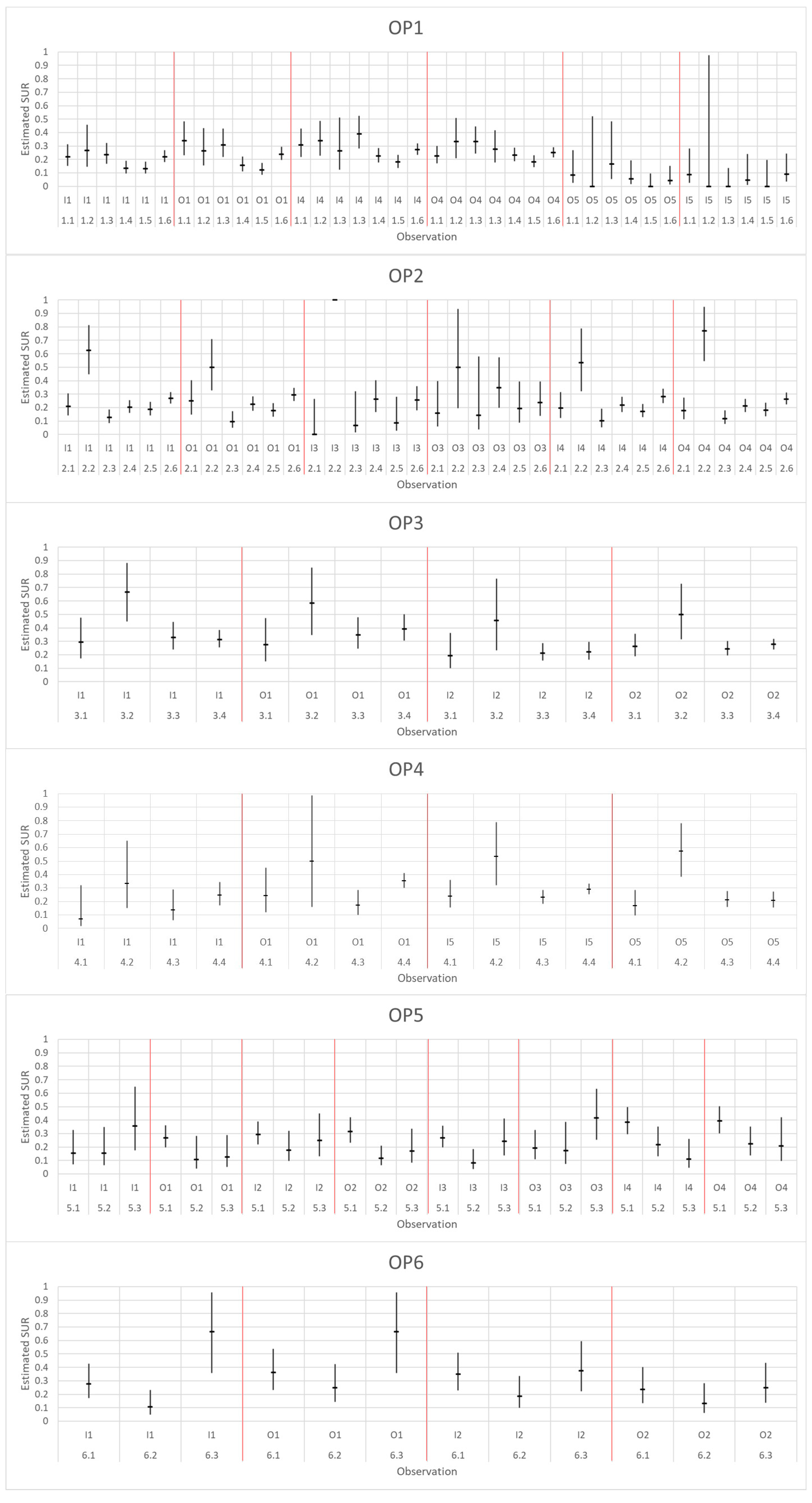
A first analysis of SUR was performed for all road segments, determining the SUR confidence intervals for all sessions. Figure 4 shows the SUR estimations, grouped by observation point. There are two horizontal axes for each plot: the upper one indicates the specific measurement location (e.g., I1, O4, etc.). The lower axis shows the observation code (see Table 1). The date was not shown instead because some days presented two data collections (i.e., in the morning and in the afternoon).

Some interesting facts can be seen about bicycle volumes and SUR patterns, which can be explained based on the location of the observation points and how cyclists perform along these roads (see Section 2.2: Data Collection).

OP1: Most cyclists coming from I1 leave the roundabout through O4. As expected, several nonprofessional cyclists enter the roundabout throughout I1, turn 180°, and return to Valencia using O1. Therefore, O4 is left for more professional cyclists. Accordingly, a higher SUR can be observed with wider intervals (i.e., lower bicycle volumes).

The observation code 1.2 corresponds to an afternoon determination of the SUR. This presents a very similar value than in the morning. In fact, the SUR for the whole observation point is quite stable, compared to other locations. A possible explanation is that Valencia city is very close to OP1. All connections to the beach (I5 and O5) presented a low cycling demand and very low SUR intervals, corresponding to people who are not willing to track their activities since their goal is just going to the seacoast.

OP2: The average SUR parameter was about 20% for all these four road segments. Less accurate estimations could be performed for I3/O3 segments, which presented quite a low demand.

OP3: The high volume of motor vehicles makes this zone undesirable for occasional cyclists. Therefore, the Strava Usage Rate is a bit higher than in other zones. Being a major junction is a key factor to explain its SUR behavior. While other observation points are occasionally covered by cycling groups, OP3 connects to many routes and therefore it is far more regularly visited. As a result, its SUR is quite stable, around 0.3 for I1/O1 and about 0.2-0.25 for I2/O2.

OP4: Due to the lower demand compared to OP3, here the SUR presents big variability, between 0.15 and 0.40 in some cases.

OP5 and OP6, both far away from Valencia and a relative low demand, present strong SUR variations depending on the day.

As a result, some factors that have proven to be related to the SUR are traffic volume and proximity to the urban zone. Previous studies on rural roads indicated that SUR ranged between 15% and 30% [39,40]. The findings confirm this range and provide additional information about the variation patterns. One important conclusion is that there does not exist a single SUR value for all road types. Moreover, the SUR also varies for a road segment within a single day, even for roads presenting high bicycle volumes.

Higher SUR values have been found at roads with a higher rate of professional cyclists. Since there is not a way to measure the professional level of a cyclist, this has been inferred from the authors’ experience and secondary aspects such as the grouping pattern of cyclists. It is in line with the findings of previous research and with the lower SUR values found by other researchers [31,32,33], who estimated the use of Strava at urban zones, where very few professional cyclists are expected).

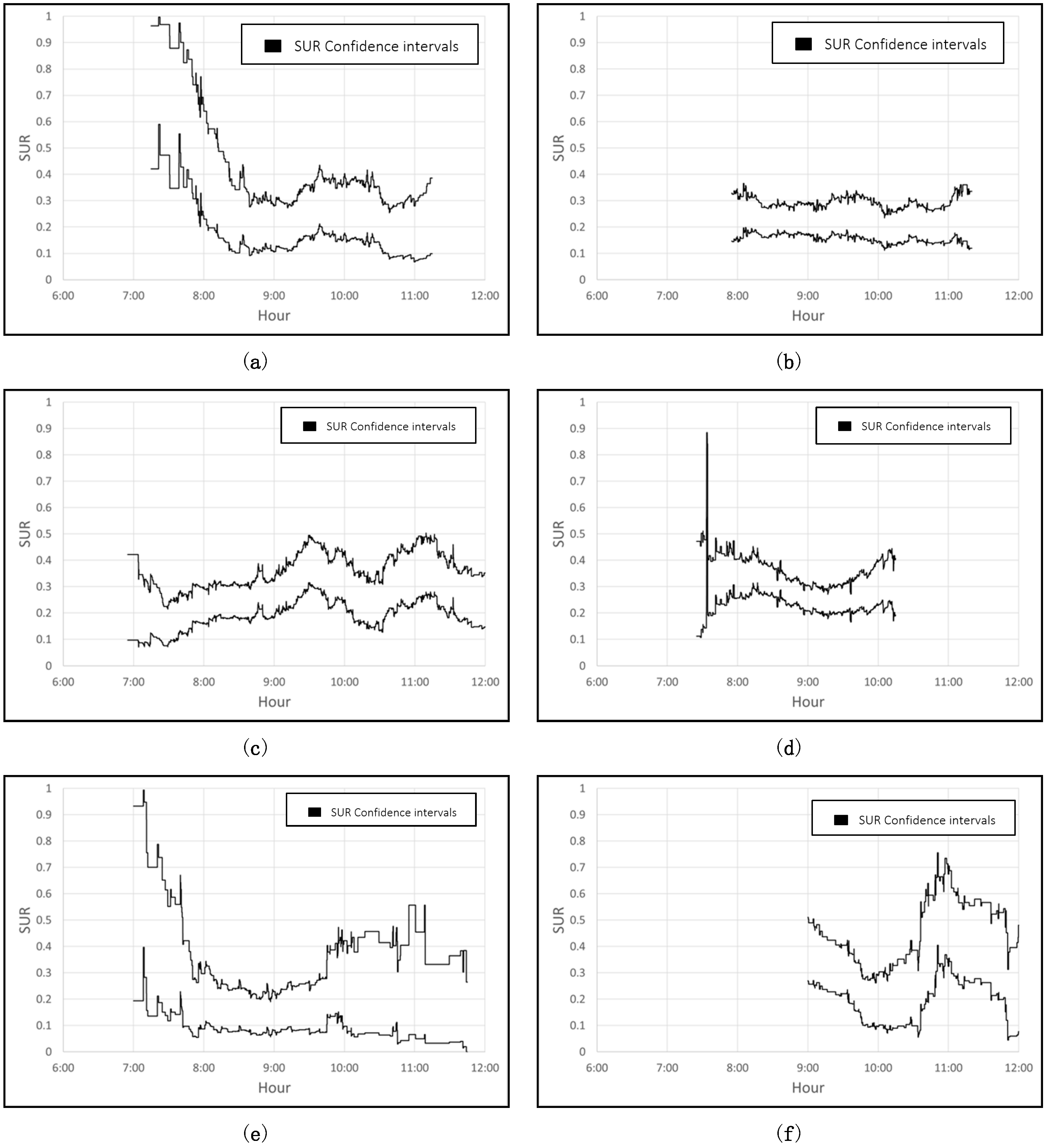
3.2. Determination of the Sliding Window Integration

In the previous section, the Strava Usage Rate variation across locations has been examined. For that analysis, the SUR was obtained for all observed cyclists within a session at once. It is also of interest to analyze how SUR varies within a day. The sliding window methodology was selected.

While motorized traffic is pretty stable and 15–60 min aggregation is normally suitable, cyclists do not behave that smoothly. Short integrations would present a noisy behavior, while very long ones would not give accurate data. Hence, it is necessary to determine which temporal aggregation provides an adequate balance between accuracy and representativity.

$\overline{SUR}$ confidence intervals profiles were determined for several road segments of the study, using different periods of time for the sliding window (Figure 5). A sliding window every second was created. These profiles were the representation of the confidence intervals of this parameter along the observation time.

Very short sliding windows led to frequent situations with no observed cyclists (Figure 5a), making difficult the determination of any $\overline{SUR}$ threshold. In addition, sliding windows with few cyclists led to very wide confidence intervals, which are not useful for the estimation of bicycle volumes. In addition, there are some moments with no cyclists at all which present abnormal confidence intervals. This can be seen in Figure 5a at about 10:09 h.

On the contrary, very long sliding windows tend to smooth subtle $\overline{SUR}$ variations (Figure 5d).

A sliding window of one hour (Figure 5c) was finally proposed as an adequate balance between these situations. However, longer windows might also be suitable for low cycling demand roads or when no important $\overline{SUR}$ variations are expected.

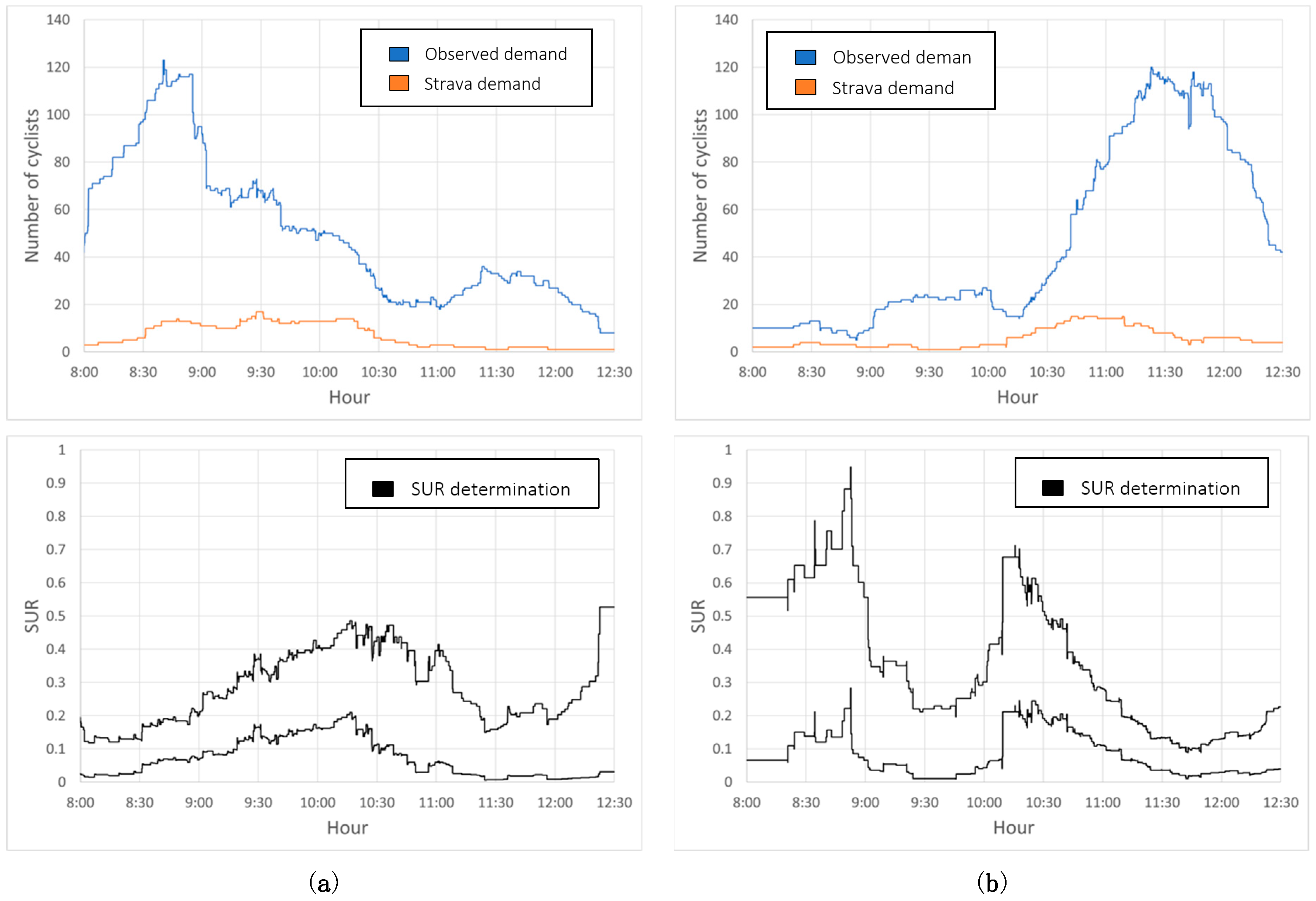
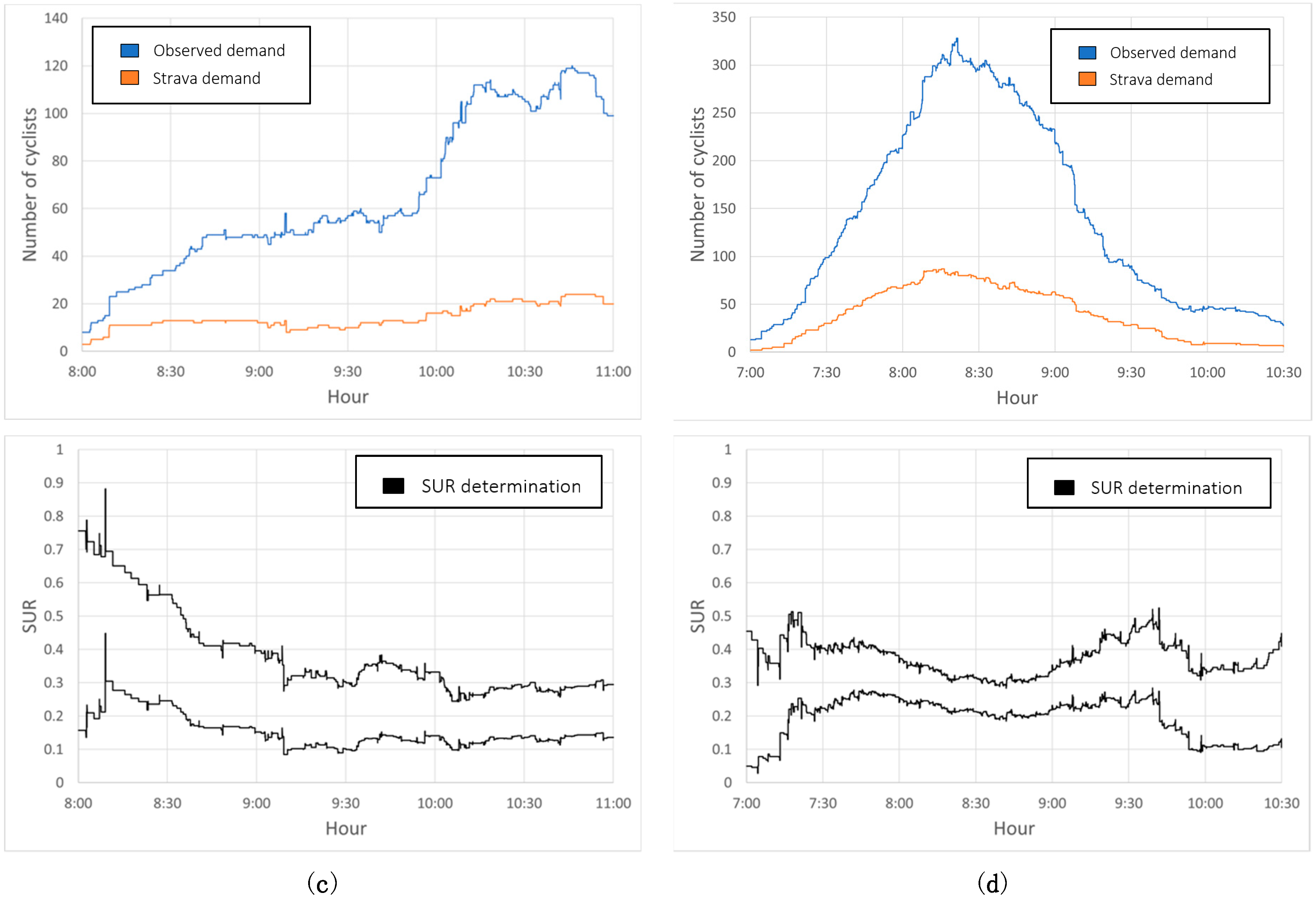
3.3. Hourly SUR Variation

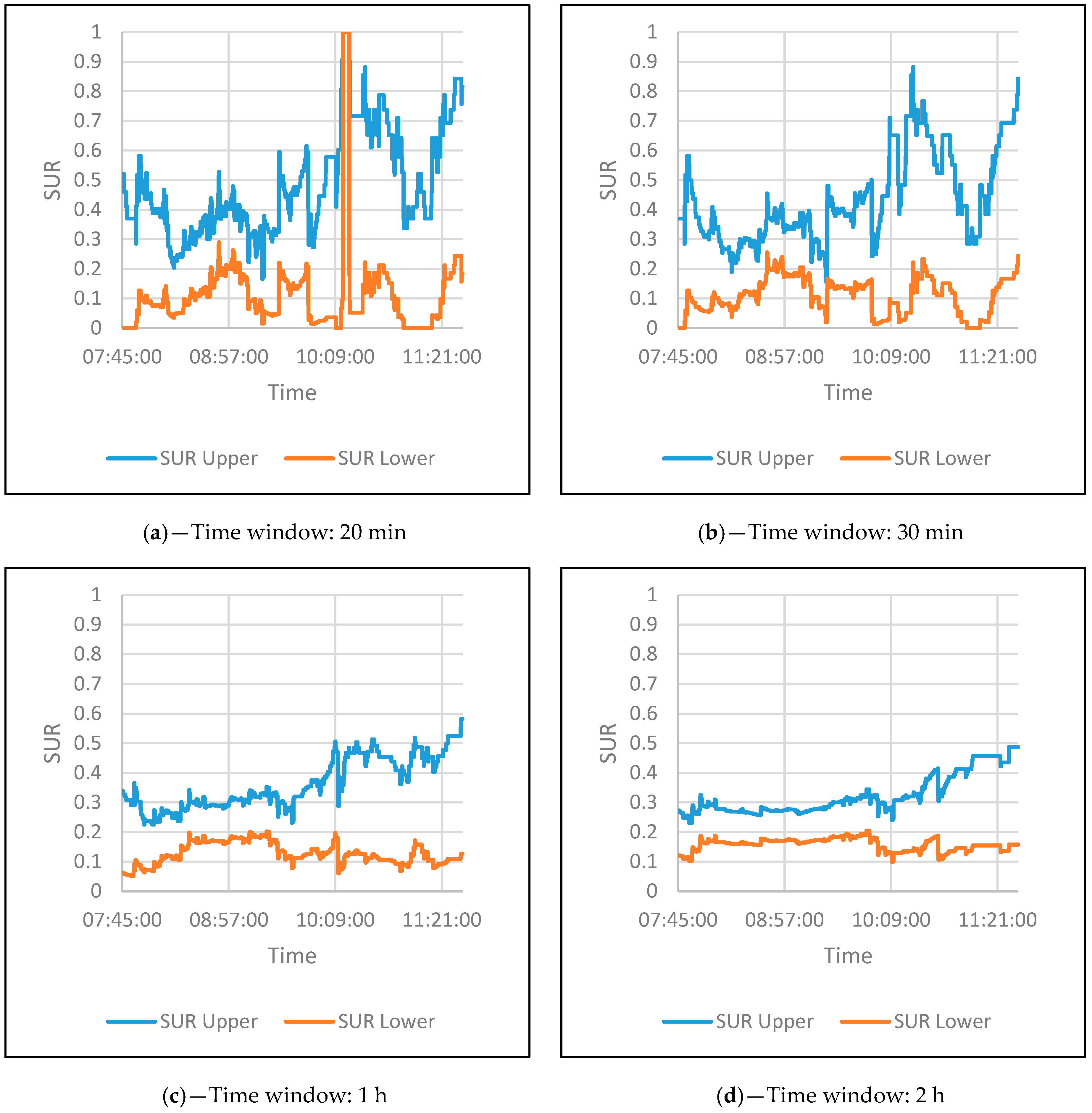
SUR profiles were depicted for all road segments under analysis. Confidence intervals were found to present important variations within every observation, due to different reasons. Figure 6 shows some relevant findings.

Figure 6a,b compare both directions for the same road segment, which is near Valencia. Regarding this, there is a huge cycling demand in the early morning for road segment I1 (exiting from Valencia), which is quite similar to a demand peak in the late morning for road segment O1 (return to Valencia). It can be observed how very low cycling demands produce wide or unstable SUR estimations. However, the SUR estimation for both peaks is very low (0.1 to 0.2 for the first case, 0.02–0.1 for the second). This is in line with the low SUR global value estimated for the whole day in the previous section.

Figure 6c shows how cycling demand is almost negligible in the very early morning, thus leading to too wide SUR intervals. As the morning advances, a higher demand is observed, and narrower SUR ranges are identified. Stabilization is around 0.15–0.30, indicating a more professional type of cyclist.

Figure 6d shows the SUR evolution for the hub intersection. The high and durable peak of demand produces a very stable SUR. As previously said, more professional cyclists are expected in this area, which is connected to the higher SUR values (ranging from 0.2 to 0.3 and even more).

Additionally, there is a huge variability of the SUR when it comes to analyzing a road segment. Sudden demand variations, discrete route choices by groups, and other factors influence this variability and prevent us from giving a standard procedure to estimate a valid SUR for a single road segment.

However, this uncertainty can be partially overcome by considering not the SUR for an individual road segment but all road segments belonging to an observation point, i.e., a road junction. This partially stabilizes minor SUR variations. Figure 7 plots some examples of this aggregation for all observation points.

4. Discussion

4.1. Estimation of AADB Using SUR

The main goal of having an accurate SUR parameter for a certain road facility is to estimate its bicycle volume. Thus, the Average Annual Daily Bicycle (AADB) volume can be estimated using SUR as expressed in Equation (10).

$$AADB=\frac{V_{Str}}{365·SUR}$$

(10)

where $V_{Str}$ is the total amount of Strava tracks in a year, and $SUR$ the calibration factor for the location.

However, a single SUR factor cannot be designated for any given specific location, since it presents hourly, seasonal, and random variations. In addition, Camacho-Torregrosa et al. [41] suggested that weekday and weekend cycling demand patterns differed significantly from each other, so a separated calibration was preferred instead of using weekend adjustment factors.

Therefore, it would be desirable to have as many SUR calibrations as possible. At first proposal of eight SUR determinations for a certain location is suggested, two per season, one at weekdays, the other at weekends. This distribution might vary depending on regional conditions, or further research that could find a SUR distribution pattern. With these eight SUR calibrations, Equation (11) allows the estimation of AADB.

$$AADB=\frac{5·AAD{B}_{WD}+2·AAD{B}_{WE}}{7}$$

(11)

where $AAD{B}_{WD}$ is the Annual Average Daily Bicycle volume for weekdays, and $AAD{B}_{WE}$ for weekends (bicycles/day). They are determined by Equations (12) and (13), respectively.

$$AAD{B}_{WD}=\frac{V_{Str,I,WD}}{n_{I,WD}·SU{R}_{I,WD}}+\frac{V_{Str,II,WD}}{n_{II,WD}·SU{R}_{II,WD}}+\frac{V_{Str,III,WD}}{n_{III,WD}·SU{R}_{III,WD}}+\frac{V_{Str,IV,WD}}{n_{IV,WD}·SU{R}_{IV,WD}}$$

(12)

$$AAD{B}_{WE}=\frac{V_{Str,I,WE}}{n_{I,WE}·SU{R}_{I,WE}}+\frac{V_{Str,II,WE}}{n_{II,WE}·SU{R}_{II,WE}}+\frac{V_{Str,III,WE}}{n_{III,WE}·SU{R}_{III,WE}}+\frac{V_{Str,IV,WE}}{n_{IV,WE}·SU{R}_{IV,WE}}$$

(13)

where $V_{Str,i,j}$ is the Strava volume for season $i$, $j$ being weekdays or weekends; $n_{i,j}$ is the number of days for every situation, and $SU{R}_{i,j}$ is the corresponding SUR factor.

Further research is still needed to determine how the SUR varies in terms of road and region. While important SUR variations might exist across road segments and locations, cycling demands have been proven to be more stable [41]. From these patterns, weekdays normally present two peaks, while weekends normally present a single peak in the morning. This information could help road authorities to plan data collection campaigns in order to calibrate SUR and bicycle volumes.

Some locations presented important SUR variations with no clear pattern. However, those with a higher demand were more stable. This is an important strength of the proposed methodology since AADB of the most important roads are more accurately estimated, providing a more accurate analysis of road safety and operation.

This study did not cover all SUR variations along a year. Data collection campaigns focused at the moments when the highest demand was expected, given their highest impact on the final AADB estimation. This implies that there are no SUR estimations for winter and bad-weather conditions. However, much lower demand has been detected for the same region, so extrapolating the SUR parameter would presumably not produce AADBs much far from reality. In any case, further research is desirable to capture this variation and provide more reliable estimations.

At weekdays, the SUR parameter might vary between the morning and the afternoon. This should be explored in further research, but it is recommended to observe bicycles during the whole session at weekdays. On the other hand, the only peak at weekends, located in the mornings, simplifies the observation session, since the morning covers most of the cycling demand. The afternoon/evening demand is nearly negligible. It is important to highlight that these are preliminary conclusions and might vary in other regions.

4.2. AADB Applications

An adequate estimation of AADB presents important advantages related to both road safety and traffic performance.

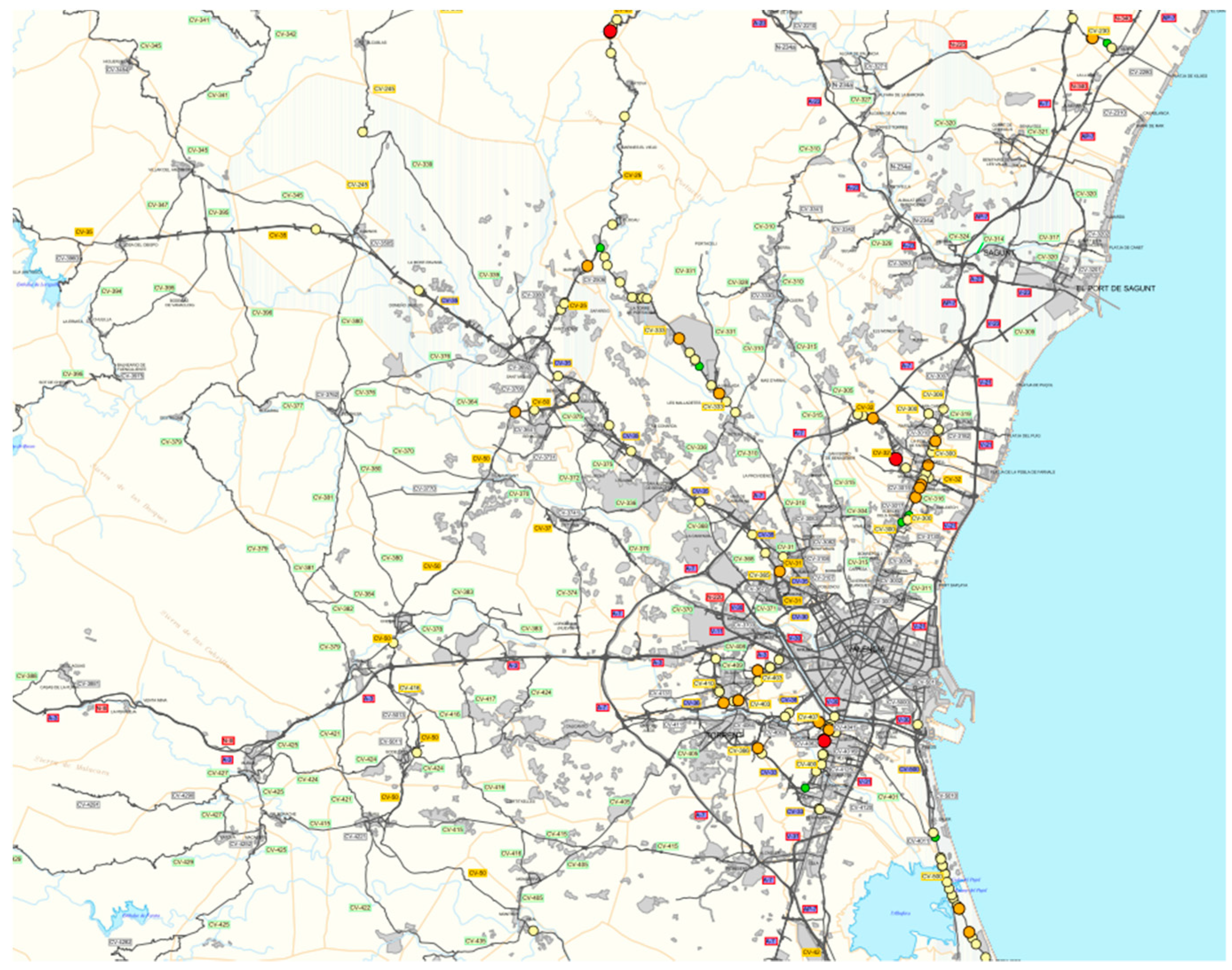
A major goal for every road traffic authority is the reduction of traffic crashes and casualties. The Valencian regional government is already tracking road crashes involving bicycles (Figure 8), which can be used to orientate mitigation measures. However, this information is not complete, since the bicycle exposure (i.e., the bicycle volume per each road facility) should be used to compare among segments.

Although not linear, there is a relationship between exposure and the number of crashes, which can be expressed as a Safety Performance Function (SPF). Once calibrated for a certain region, this function is useful for both new and existing road segment facilities:

(a)

For new road segments, the SPF can be used to estimate the expected number of crashes involving bicycles (AADB should be estimated first). This estimation would be more accurate if more factors are included in the SPF.

(b)

For existing road segments, the SPF outcome can be compared to the observed crashes. If there are more crashes than estimated by the SPF, the road segment produces more crashes than expected, so special countermeasures should be applied. On the contrary, if the SPF estimation exceeds reality, the road segment should be studied to determine which factors are enhancing safety. In both cases, only extreme differences should be considered, provided that the SPF is fitting real data and therefore presents some error.

SPFs, thus, are a powerful tool but a large amount of data is required. If not present, Highway Administrations could use AADB and crash data to determine the average crash rate for a given type of roads. Again, road segments showing a crash rate above the average should be targeted by these administrations to enhance road safety. An effective countermeasure prioritization should be made in terms of potential for improvement (i.e., effective number of crashes that could be saved thanks to a given intervention).

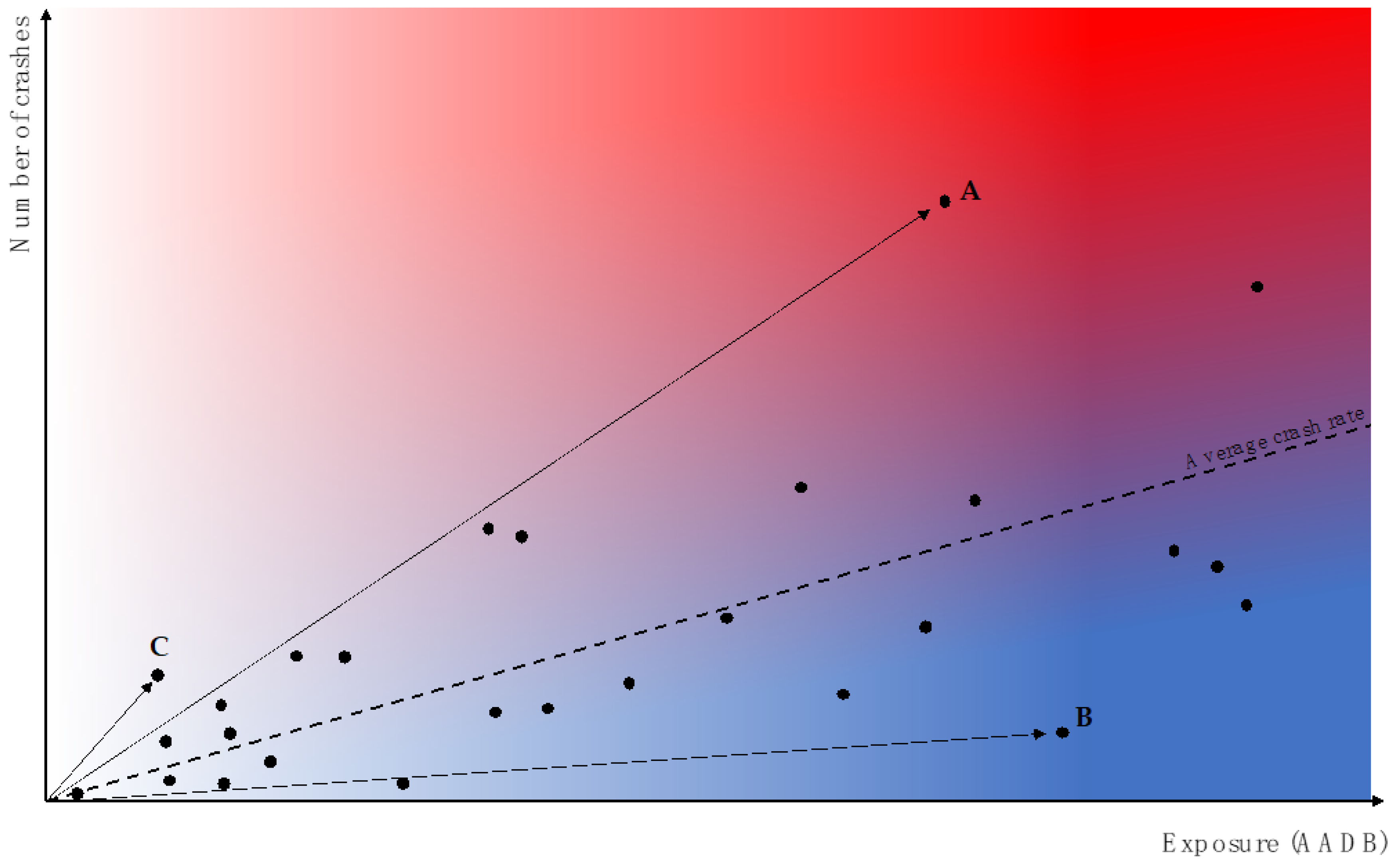
To express this concept, Figure 9 shows how road crashes and bicycle exposure (AADB) are related. Every single point represents the AADB-crash relationship for a single road segment. These are not real data and have just been provided to show the concept. Moreover, real data remains unknown to us due to the lack of accurate AADB data for an extensive part of the road network.

Among all different road segments, three of them have been highlighted to show how a road administration should proceed, as a function of their AADB-crash relationship:

• Road segment A presents a high AADB and a higher-than-the-average number of crashes. This segment should be a priority for road authorities, since it presents quite more crashes than the average road segment with the same AADB. The difference between the observed crashes and the average crashes for the same AADB is the potential for improvement.
• Road segment B presents also a high AADB, but the number of crashes is quite below the average for the same AADB. The road authorities should analyze why this happens and export the conclusions to other road segments (if possible).
• Road segment C presents a very high crash rate (slope of the arrow connecting this point to the origin). Although this crash rate is even higher than for road segment A, road segment C should not be a priority compared to road segment A, given its lower potential for improvement.

This analysis is a little bit simple since it does not consider other factors such as the cost of the measures and the actual potential for improvement (which can only be obtained by estimating the safety outcome of the implemented countermeasures). In addition, the motorized traffic volume and all other crash types should also be considered to take the actions. However, it provides a general overview of how cycling exposure could be considered to improve safety.

Roads that present high bicycle volumes might also present problems on traffic performance, due to the speed disparity to motor vehicles. Thus, an adequate calculation of AADB would help road authorities better estimate traffic performance and level of service.

5. Conclusions

To enhance road safety and operation on two-lane rural roads where the number of bicyclists is constantly rising, it is necessary to know or estimate cycling demand. Although the use of the bike in urban areas is very heterogeneous (e.g., leisure or commuting), bicyclists ride on two-lane rural roads mainly for fitness training, often using sport crowdsourcing apps such as Strava to save and share their activities.

This research presents a novel methodology based on the analysis of the daily evolution of the Strava Usage Rate (SUR) on two-lane rural roads in order to enhance the estimation of the Annual Average Daily Bicycle (AADB) volume.

Specifically, an analytic analysis of the SUR confidence intervals was carried out. It was identified that the SUR reliability largely depends on the number of observed cyclists. In this way, the greater the cycling demand, the more accurate the SUR determination and, consequently, the estimation of AADB.

The SUR variation on 32 road segments was studied. Some important conclusions were obtained: (1) locations with higher cycling demand are expected to present more stable SUR, (2) higher SUR values are connected to a higher rate of professional cyclists, and (3) determining SUR for an entire road junction might provide more stable SUR estimations than for single road segments.

Based on these findings, some indications to calibrate the SUR and to use it for AADB estimation can be provided. A first SUR ranging between 20% and 30% could be first set to estimate AADB solely based on data from the web of Strava. This would help identify the target locations where the cycling volume might be remarkable. Road authorities could then focus on these road facilities, establishing specific count campaigns to calibrate this parameter, where needed. A reasonable number of eight counts have been proposed. The count duration should vary according to the proximity to important cities or the road type. It is important to highlight that the objective of having a SUR calibrated is to estimate cycling without the need to perform additional counts, which would be too time consuming. This parameter should be updated along the years. In addition, Strava has been used due to its popularity, but other platforms might be used as well, with different representativity.

A good AADB estimation would help road authorities to take better decisions in cycling network planning, design, and management. Specific safety measures for cyclists could be applied to the most demanding roads; or the crash/AADB ratio could be used as an indicator of cycling safety. Further research would be desirable to examine seasonal SUR patterns, including more observation points.