Functional Resonance Analysis in an Overtaking Situation in Road Traffic: Comparing the Performance Variability Mechanisms between Human and Automation

Abstract

Automated driving promises great possibilities in traffic safety advancement, frequently assuming that human error is the main cause of accidents, and promising a significant decrease in road accidents through automation. However, this assumption is too simplistic and does not consider potential side effects and adaptations in the socio-technical system that traffic represents. Thus, a differentiated analysis, including the understanding of road system mechanisms regarding accident development and accident avoidance, is required to avoid adverse automation surprises, which is currently lacking. This paper, therefore, argues in favour of Resilience Engineering using the functional resonance analysis method (FRAM) to reveal these mechanisms in an overtaking scenario on a rural road to compare the contributions between the human driver and potential automation, in order to derive system design recommendations. Finally, this serves to demonstrate how FRAM can be used for a systemic function allocation for the driving task between humans and automation. Thus, an in-depth FRAM model was developed for both agents based on document knowledge elicitation and observations and interviews in a driving simulator, which was validated by a focus group with peers. Further, the performance variabilities were identified by structured interviews with human drivers as well as automation experts and observations in the driving simulator. Then, the aggregation and propagation of variability were analysed focusing on the interaction and complexity in the system by a semi-quantitative approach combined with a Space-Time/Agency framework. Finally, design recommendations for managing performance variability were proposed in order to enhance system safety. The outcomes show that the current automation strategy should focus on adaptive automation based on a human-automation collaboration, rather than full automation. In conclusion, the FRAM analysis supports decision-makers in enhancing safety enriched by the identification of non-linear and complex risks.

1. Introduction

In the past, traffic safety was improved by three major safety strategies including engineering, enforcement, education [1], and their intertwinings. Nevertheless, according to the World Health Organisation [2], over 1.2 million people die each year on the world’s roads, and between 20 and 50 million suffer non-fatal injuries. These are still high numbers that need to be improved. A promising countermeasure seems to be a technology advancement by automated driving (AD, Level 3 and higher, according to SAE J3016 [3]), which offers great possibilities in traffic safety enhancement. A frequent argumentation for this assumption is that the human in his role as a driver is the main cause of accidents, claiming that human error causes approximately 90% of road crashes, e.g., [4,5,6,7]. Consequently, it is frequently recommended that the human driver be removed from the system and road accidents will probably decrease by 90%. The common idea behind this is that technology can be introduced into a system by simply substituting machines for people so that the system as a whole improves and there are no negative side effects. Unfortunately, this is a persistent oversimplification fallacy, also called substitution myth [8,9].

This is in accordance with Rasmussen [10], who claimed that for a general understanding of system behaviour, we do not have to focus on human errors, rather on mechanisms shaping the behaviour in the system and its context. This is also in line with Woods and Dekker [8], who stated that it is not sufficient to build a new mature system or technology and then to test and assess its performance at the tail of the design process. Rather a proactive approach at the beginning has to steer the design into a direction that considers the usefulness of a potential new system given the possibilities new technology provides and anticipates how technology transforms the nature of practice. Probably, this would facilitate a system performance enhancement. Moreover, this is consistent with insights by Ackoff [11], who stated that in any system, when one improves the performance of the parts taken separately, the performance of the whole does not necessarily get improved because the way the parts fit together determines the performance of the system and not on how they perform taken separately. Thus, a system is not the sum of the behaviour of its parts, it is a product of their interactions. Further, Grabbe et al. [12] designate the frequent argumentation of AD as too simplistic thinking that falsely links the logic of a clear causal link. Rather, according to Bengler et al. [13], the human driver is both an active and passive participant in an accident, as well as accident avoidance and compensation element in the same system. Consequently, a more differentiated view is required to improve the safety of the entire road system through the efficient interaction between humans, machines, and other road users.

Therefore, according to Grabbe et al. [12], the very first step in the development process of automated vehicles is to understand the mechanisms of accident development and accident avoidance in road traffic. Hence, the driver’s contribution in the corresponding situations can be assessed to derive requirements for automation and the potential of automation with its accompanying factors. Thus, the understanding of the mechanisms of the road system is essential. Otherwise, adverse automation surprises, as happened in other domains such as aviation, e.g., [14,15,16,17], will probably occur due to safety blind spots [18] and could ultimately develop into a “showstopper”. This raises the question of: which methods are best suited to reveal the safety mechanisms in road traffic? To clarify the question, Grabbe et al. [12] reviewed the historical development of accident analysis models, the properties of the road system, and a common understanding of safety. In the following, a brief overview of their analysis and main conclusions is given.

According to Hollnagel [19], three different and major accident models can be distinguished: sequential, epidemiological, and systemic. Sequential accident models describe the accident as the result of a chain of discrete events occurring in a particular time sequence. Here, losses are caused by technical failures or human error, assuming that the cause-and-effect relationship is linear and deterministic [20]. Then, the focus changed with introducing the epidemiological models to an organisational level, where accidents result from a combination of different interacting factors [20]. This improved the understanding of accidents regarding complexity, but the causality is still linear and the links between states are loose, which that does not adequately represent the dynamics of a system [21]. Thus, systemic models arose seeing the accident process as a complex and interwoven event that cannot be broken down into its individual parts [22] and rather analysing interactions within the whole system. Salmon et al. [23] concluded that the road system, which connects technical, human, and social elements to transport people and goods from one place to another, is of a socio-technical nature. Additionally, they also argued in favour of a complex system based on the prerequisite properties of complexity presented by Dekker et al. [24]. Further, Perrow [25] defined a framework called interaction-coupling matrix to classify systems based on their system characteristics. Here, systems can be generally distinguished by the two dimensions of interaction and coupling. The interactions can be linear or complex and the couplings are loose or tight, which results in four quadrants of system assignments. In particular, a socio-technical system (STS) can be described by an increasing number of tight couplings and complex and non-linear interactions [25]. Wienen et al. [22] extended this framework by combining it with the three types of accident models mentioned above. Based upon this, Grabbe et al. [12] classified the road system as a system with highly complex interactions and tight couplings assigning it to the systemic quadrant within the matrix. Consequently, they concluded systemic methods are best suited to represent a safety assessment of AD and especially reveal mechanisms in road traffic. This is also confirmed by the analyses of Larsson et al. [26] and Hughes et al. [27] claiming that system theory and systemic models are an important and major basis for safety work in road traffic. Furthermore, safety is a complex issue, and many different views exist, providing a variety of measures giving a reasonable description. So, every view captures some elements of safety but not the entire picture [28]. Thus, safety cannot be defined by one clear definition or construct. However, the historical development of the scientific study of safety points out two fundamental concepts where safety is concerned: the traditional thinking about safety, also called safety-I [29], which is based on the Newtonian and reductionist approach [30], and the modern view of risk and safety management, also called safety-II [29], which follows a complexity-oriented holistic approach [31] based on Resilience Engineering (RE) [32]. A critical perspective on the two safety perspectives concerning AD and road safety by Grabbe et al. [12,33] unveiled that the safety argumentation, as well as the safety assessment of AD, is largely safety-I driven, and the safety-II perspective is strongly neglected. Thus, they requested an urgent application of this safety view. This is also in line with Hollnagel’s [34] (last slide) general statement regarding safety management that “it is an unavoidable dilemma that we inadvertently create the challenges of tomorrow by trying to solve the problems of today with the mindset (models, theories & methods) of yesterday”.

Since systemic analysis methods, as well as a safety-II perspective, seem best suited to identifying the safety mechanisms in road traffic against the background of AD, Grabbe et al. [12] extensively compared the major systemic methods and discussed their benefits and limitations. The authors recommended using the functional resonance analysis method (FRAM) at the very beginning of a product development cycle, concluding that FRAM is the most adequate method to reveal the safety mechanisms in road traffic. This is also supported by Ferreira and Cañas [35], who see FRAM as a useful tool to build an understanding of the actual system mechanisms and workings that are needed to support the risk management concerning the proactive assessment of technological changes and their impacts. Apparently, there is no “one-size-fits-all” solution to safety, which is especially true for complex and dynamic STS. Thus, overall, we need combinations of different views, approaches, and measures including safety-I and safety-II. However, a significant perspective, that is RE, is currently lacking and inevitable as a fundamental basis for the safety assessment of AD. Here, FRAM, which is based on RE, is the most recent and promising step to understanding STS [36]. Therefore, Grabbe et al. [12] investigated the applicability of FRAM in a case study to evaluate its suitability in more detail with regard to a purely methodical process. They discussed several strengths and limitations. Ultimately, the authors concluded that the safety challenge of AD requires the study of interactions and mechanisms of the road system where FRAM adequately addresses these issues considering this method a “missing piece in the puzzle” for a risk assessment of AD, which potentially helps to reveal hidden risks or safety blind spots of AD.

To continue this research and to reduce the research gap in the safety assessment of automated vehicles regarding the aforementioned perspective, this paper aims to identify the mechanisms of road traffic in one specific scenario, that represents a huge potential to increase safety through automation in a complex setting, by using FRAM. Hence, these mechanisms can be compared between a human driver and a highly automated vehicle, which allows us to evaluate the contributions of the human driver and the automation. Finally, system design recommendations for AD, considering potential accompanying factors as well as insights for the validation process, reducing its effort, can be delivered in order to show how FRAM can be used for a systemic function allocation for the driving task between humans and automation.

The remainder of this paper is structured as follows. Section 2 summarises the theoretical foundations and individual analysing steps of FRAM, as well as its applications. Section 3 describes the implementation of the overall methodological research process and its individual steps in detail. In Section 4, the results are presented including the FRAM model of the analysed scenario, the identification of the contributions by the human driver and the automation to the safety of the system, and recommendations for system design as well as the validation process of AD. Then, Section 5 discusses the results with respect to the research goals and also outlines methodological issues. Finally, a brief conclusion and outlook for future research are given in Section 6.

2. Functional Resonance Analysis Method

FRAM [37] is basically a qualitative method for risk assessment and accident analysis. It allows the modelling of mechanisms within a complex STS, including their interfaces between humans and technology, coupling and dependency effects, nonlinear interactions between elements, and functional variability [38]. The purpose of the resulting model is to analyse how something happens or how a system works as work-as-done (WAD). In particular, the description and understanding of the STS are given in terms of functions rather than components. A FRAM model focuses on adjustments to everyday performance, which usually contribute to things going right. Rarely, these performance adjustments aggregate in unexpected ways, functional resonance will occur, and accidents are the most extreme result. The ultimate objective is not to eliminate performance variability but to investigate and monitor what is necessary for everyday performance to go right, trying to dampen variability in order to reduce resonance effects and unwanted outcomes [37]. In general, the results of a FRAM analysis contribute to the understanding of real work and unveil unsafe functional interactions within one agent and between different agents that are often underestimated by traditional methods and design approaches [35,39].

FRAM follows four principles (i.e., the equivalence of success and failures, approximate adjustments, emergence, and functional resonance), and four steps (i.e., modelling the system through identifying its functions, identifying the function’s performance variability, aggregating the variability, and managing the variability) are required for its analysis as detailed in Hollnagel [37]. The steps are briefly described in the following. In the first step, the essential functions of the system ensuring the success of everyday work are identified to build a model. These functions produce a certain outcome referring to tasks as work-as-imagined (WAI) or activities as WAD. Each function is characterised by six aspects (i.e., input, output, precondition, resource, control, and time), which couple each function with several other functions representing a specific instantiation of the model. The resulting model is traditionally represented graphically by hexagons depicting each function with its six aspects. Furthermore, the functions can be divided into two classes: foreground and background functions. Foreground functions are the focus of the analysis and may vary significantly during an instantiation of the model. In contrast, background functions are stable and represent common conditions as system boundary that are relevant for and used by foreground functions. The second step is to identify and specify the performance variability of each function. This is crucial to understand how the variability can propagate through the system by the couplings between functions, which can lead to unwanted outcomes. After the identification process, the variability has to be characterised using different variability manifestations, the phenotypes. The simple solution considers two phenotypes, these are timing and precision, where the function’s output in terms of timing can occur too early, on time, too late or not at all, and in terms of precision, the output can be precise, acceptable, or imprecise [37]. As it is not enough to simply know the variability of individual functions in isolation, the third step in FRAM is to aggregate the variability to know where functional resonance emerges. This is done by defining upstream-downstream couplings where variability can be caused through couplings of upstream functions, when the output used as, for example, input or precondition is variable and thus affects the variability of downstream functions. This impact is likely to lead to an increase in variability (amplifying effect), a decrease in variability (damping effect) and to maintain variability (no effect). The last and fourth step consists of the monitoring and management of the performance variability that was identified in the previous steps. This step aims to manage or dampen variability to a level where no unwanted outcomes arise, rather than eliminating variability since this is inevitable for things going well in complex STS. Finally, this ensures the safety and performance of the system. The implementation of each step is more detailed in Section 3.

In the past, FRAM has been widely used, applied, and enhanced methodologically in a variety of domains for retrospective as well as prospective analyses, as detailed in a comprehensive review by Patriarca et al. [40]. Hence, FRAM has been progressively evolved since its starting point in 2004. The main application fields include aviation, e.g., [41,42,43], healthcare, e.g., [44,45,46], industrial operations in plants, e.g., [47,48,49], the oil and gas industry, e.g., [50,51], and maritime, e.g., [39,52,53] and rail transport, e.g., [54,55]. However, the context of road safety has seldom been addressed by FRAM. Here, applications refer to road safety management in a case study in Myanmar [56], a comprehensive comparison of FRAM with other systemic methods regarding the safety mechanisms in road traffic, as well as a thorough investigation of FRAM’s applicability in a case study evaluating its suitability with regard to a purely methodical way against the background of the impact of introduced automation [12], and a safety analysis of conditional automated driving including the human-machine collaboration in the event of an authority transfer from the automated system to the human driver in time-critical situations [57].

3. Research Method

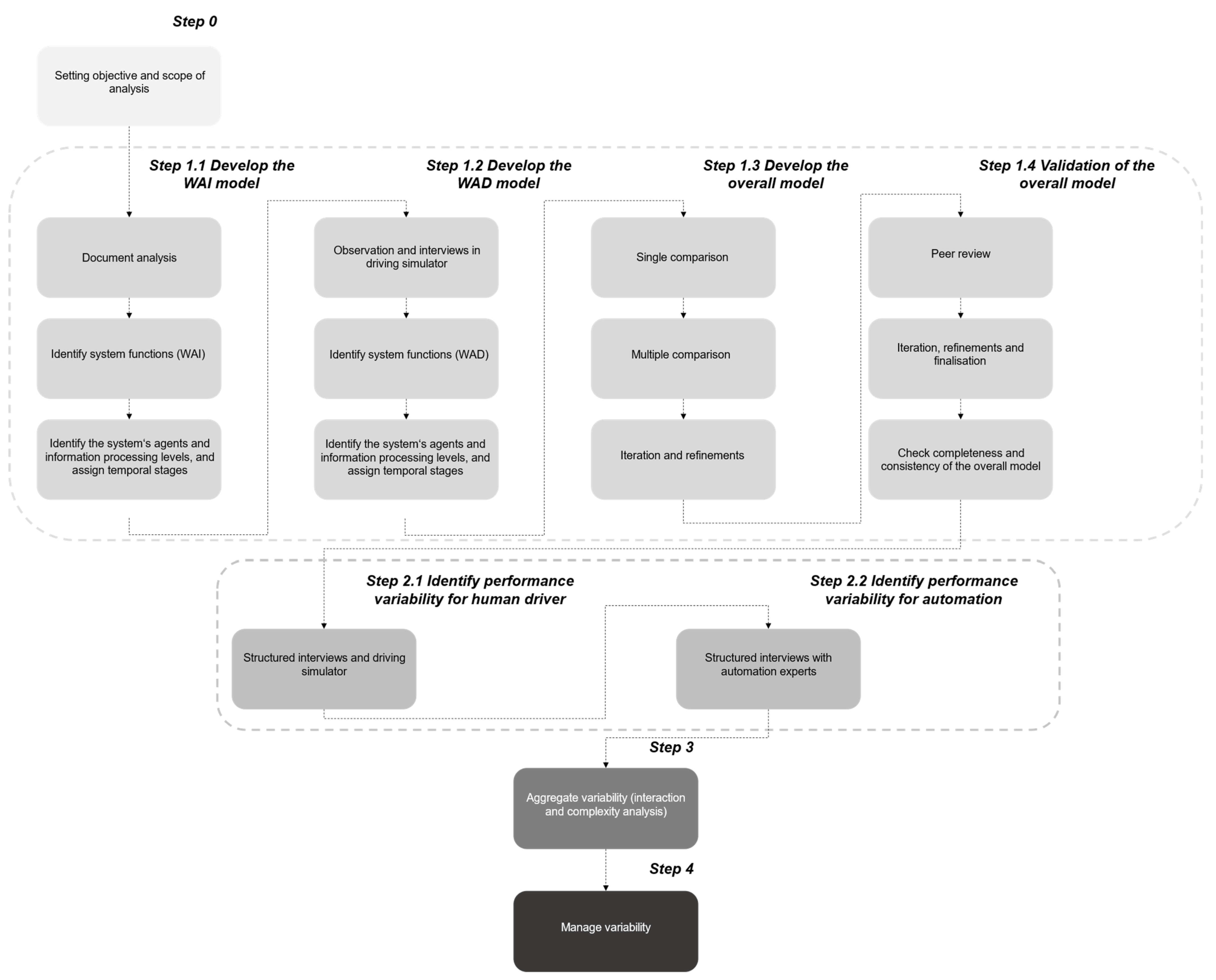
3.1. Overall Methodology

As mentioned above, FRAM is a qualitative research method, which implies that classical statistical procedures applied to quantitative methods are not adequate to meet the three quality criteria in quantitative terms of internal and external validity, reliability, and objectivity. To overcome this issue, we applied the approach of Anfara et al. [58], translating the quality criteria in qualitative terms into credibility, transferability, dependability, and confirmability in order to better assess the research quality and rigour in this study and thus to improve their trustworthiness. Additionally, Creswell and Miller [59] identified several verification strategies to comply with the four qualitative terms, where Creswell and Poth [60] recommended that at least two of these strategies be used in any qualitative study. The assignment of the quality criteria in quantitative and qualitative terms, as well as their verification procedures, can be taken from

Table 1. Assignment of the quality criteria in quantitative and qualitative terms as well as their verification procedures based on Anfara et al. [58] and Creswell and Miller [59].

Quantitative Term	Qualitative Term	Verification Strategies
Internal validity	Credibility	Prolonged engagement in field; Use of peer debriefing; Triangulation; Member checks; Time sampling; Persistent observation; Clarifying researcher bias
External validity	Transferability	Provide a thick description; Purposive sampling
Reliability	Dependability	Create an audit trail; Code-recode strategy; Triangulation; Peer examination; Stepwise replication
Objectivity	Confirmability	Triangulation; Practice reflexivity

. Here, the verification strategies underlined boldly are implemented in this study to fulfil the four qualitative terms.

As described in Section 2, the FRAM method comprises four main methodological steps. These steps and their underlying substeps are shown in Figure 1. The aforementioned quality criteria and verification strategies are intertwined in these steps. The following subchapters will explain the respective steps in detail.

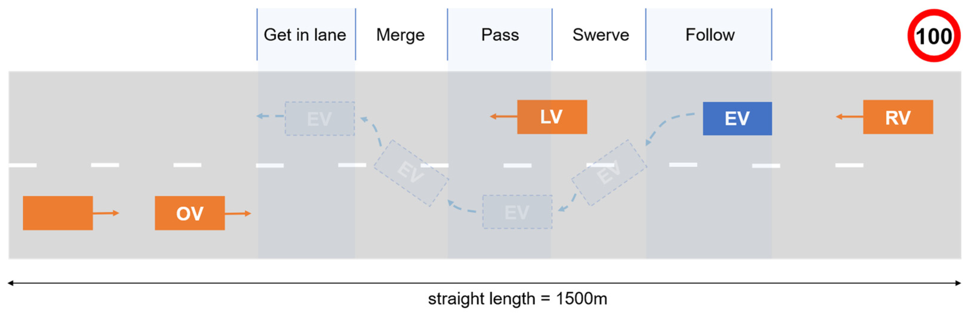
3.2. Step 0: Selection and Description of Scenario: Setting the Objective and Scope of Analysis

In this work, FRAM was used as a method for a qualitative/quantitative proactive risk assessment. Thus, the scope of analysis and the degree of resolution have to be described to set the scene and system boundary for the four steps that follow. In particular, a scenario-based analysis was conducted to compare the contributions between a human driver and AD and to evaluate their potential effects in order to improve the system design. The scenario is described below.

The scenario selected was an overtaking manoeuvre on a rural road. The main reasons are as follows. First, accidents in the city and on rural roads are by far the most critical, considering the accidents according to their location concerning frequency and severity in Germany. Furthermore, 58% of all fatal accidents in 2018 in Germany occurred on rural roads. Second, on rural roads, collisions with oncoming vehicles and leaving the carriageway pose the greatest danger [61]. By far the largest proportion of collisions with oncoming vehicles is caused by overtaking manoeuvres [62]. Therefore, overtaking situations represent accident black spots on rural roads, offering great potential for road safety improvement. Additionally, overtaking situations are classified as a relevant scenario category for a scenario-based validation of AD [33]. Third, according to Netzer [63], overtaking is a very complex traffic process with a variety of influencing factors involving several different subtasks, such as swerving, adjusting speed, merging, and the interaction of at least two drivers. Thus, this scenario offers a great potential to highlight the interaction and complexity of road traffic, including the systemic interdependencies between different road agents and the environment. In addition, results might be transferred to other road traffic scenarios because overtaking situations make up a large part of everyday driving tasks. Overall, the overtaking situation on rural roads is a good starting point for a socio-technical analysis under the lens of RE.

Figure 2 schematically depicts the overtaking scenario. This consists of four road users or agents: the ego vehicle (EV), the lead vehicle (LV), the rear vehicle (RV), and the oncoming vehicle (OV). Behind the OV, identified by the second orange and unlabelled vehicle, other vehicles form a line of cars. However, these vehicles and drivers are not considered agents for the modelling and scope of analysis and are therefore out of system boundary. To get a better overview, the scenario can be divided into five temporal and spatial stages from EV’s point of view (see Figure 2): following a vehicle in front, swerving into the oncoming lane, passing the leading vehicle, merging back into the starting lane, and getting in the lane again.

The four agents are driving on a straight rural road for a distance of 1500 m with no vertical elevation, on which the maximum speed limit is 100 km/h, overtaking is permitted and no obstructions exist. One lane runs in each direction and the median is dashed. The total width of the road is 6 m. The road is well constructed and all necessary road markings are in place. On the side of the road, there is light vegetation. The weather conditions are sunny and dry.

The EV is following the LV and at the same time followed by RV. The LV is driving at a speed of 80 km/h. In the oncoming traffic, a vehicle OV and following vehicles are coming towards at 100 km/h with different time gaps. In principle, the OV represents the oncoming traffic. All agents always keep the necessary safety distance to their vehicle in front and comply with the traffic regulations. The EV is under time pressure and wants to reach its destination quickly, and since LV is travelling below the speed limit, it starts an overtaking manoeuvre. The other agents are reacting to the overtaking manoeuvre of EV. In general, the EV is driven once by a human driver and once by an automated system (SAE-level 4) according to SAE J3016 [3] with no car-to-x communication. The other vehicles are always driven by a human driver in both cases. Overall, the overtaking scenario should represent a simple and everyday overtaking manoeuvre on a rural road, in which four road users are interacting primarily with one other. This represents a scenario in which most overtaking accidents occur, that is a straight flat section in daylight and on a dry rural road, all in all, under good external conditions [62].

3.3. Step 1: Identification and Description of the System’s Functions

3.3.1. Develop the WAI Model

The WAI model is based on a comprehensive and detailed hierarchical task analysis of driving developed by Walker et al. [64]. This work is created on a task analysis conducted by McKnight and Adams [65] in 1970, the UK Highway Code, several driving standards and manuals, input by subject matter experts (SMEs), and numerous on-road observation studies. The tasks and plans are constructed using logical operators such as And, Or, If, Then, Else, While, and so on. The list of tasks and plans, which are essential for the overtaking scenario, were translated into functions where the logical operators were used to define couplings between each function through their aspects. First, a WAI model was created for each agent, followed by a WAI model combining all agents in one model assigned to the five temporal stages of the scenario. In addition, the functions were labelled and distinguished by different information processing levels.

3.3.2. Develop the WAD Model

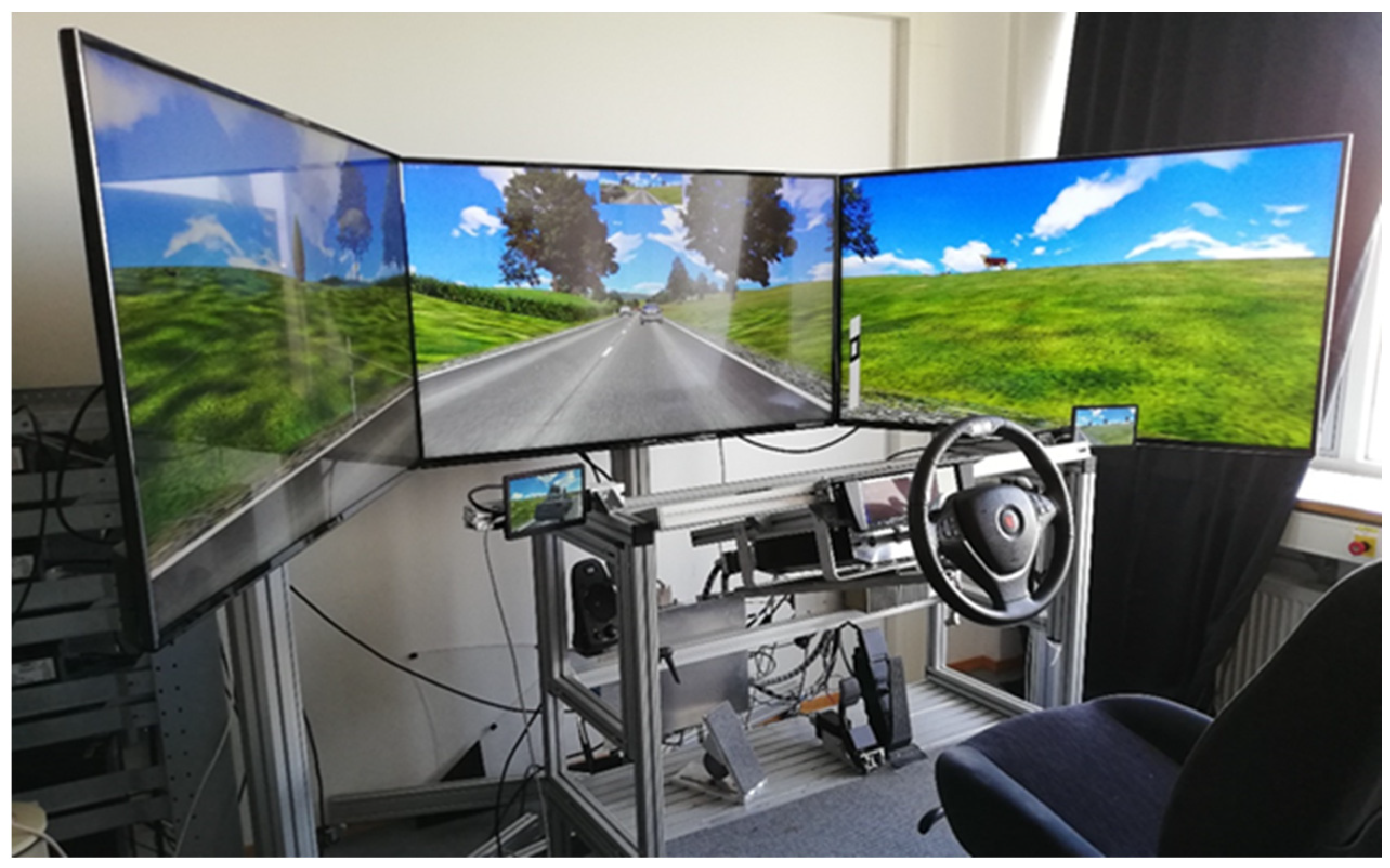
Since it is not sufficient to know only the theoretical mechanisms of the overtaking process, the next step is to create a WAD model using observations and interviews implemented in a driving simulator study which serves to update and enhance the WAI model into a more realistic overall model.

Driving Simulator

Here, a static driving simulator (see Figure 3) was used. The environment is simulated by three flat screens with a resolution of 4K covering the space from the left-side window to the right-side window of the car, which ensures a 120° viewpoint in front. Additionally, the rear-view mirror is virtually displayed at the top of the centre screen. The side mirrors are displayed via two small monitors placed to the left and right of the subject. The driver, seated on a default automobile seat that is adjustable in height and longitudinal direction, has a steering wheel for lateral control that can be adjusted along the axis, as well as an accelerator and brake pedal for longitudinal control. The use of a turn signal and a shoulder view to the rear are not possible. Behind the steering wheel is a combination display that shows the engine speed and the current speed of the vehicle. Further, the driving simulator is equipped with automatic transmission and sound, consisting of engine, environmental, and vehicle noises that are reproduced via two speakers placed next to the pedals. During a test drive, the room was darkened to increase the immersion for the driver. SILAB 6.0 of the Würzburg Institute for Traffic Sciences GmbH in Germany was used as the simulation software.

Sample

A total of 10 participants took part in the study. Of these, seven were men and three were women with an average age of 28 years (SD = 2.26 years), ranging from 24–31 years. All owned a valid driving licence and drive an average of 18,000 km a year (SD = 10,055 km/year), which shows a solid experience in road traffic. Furthermore, all subjects have already participated in a driving simulator test and were well acquainted with the driving simulator, which is why it can be assumed that their real driving behaviour has not changed much in the driving simulator. This is consistent with the indication that 80% would perform similar driving manoeuvres and overtaking manoeuvres in reality. The driving styles were heterogeneous, ranging from safe and leisurely to slightly risky and fast-paced, which was surveyed using a 5-point Likert scale.

Procedure

First, the subjects were informed about the goals and content of the study and signed an informed consent. Afterwards, the subjects took a seven-minute test drive, which included everyday driving scenarios on rural roads, to learn about steering, braking, and the driving simulator system. Then the actual test drive began. Here, the driving data, as well as the audio track and the subject’s behaviour, were recorded for evaluation. In total, the experiment lasted 30 min, and each subject experienced the scenario from the perspective of each of the four agents, in which the order of perspectives was as follows: EV, LV, RV, OV. The subject passed through each perspective three times. The first pass of the overtaking manoeuvre was used for familiarisation, during the second the subjects were asked to think aloud and explain their actions over the following few seconds, and during the third pass, the simulation was stopped five times (which represented the five stages of the scenario, see Figure 2) whereupon the subjects were asked to explain in detail which functions they would perform over the next few seconds. The functions refer to the three information processing levels of perception, cognition, and action. Between the actual test scenarios, that is the overtaking manoeuvre on the straight rural road, the test subjects each drove a small winding course through a wooded area so that the entire scenario would appear as natural as possible. After the test drive, subjects completed a short questionnaire to collect demographic data. Additionally, driver type data, as well as perceptions in the driving simulator test, were surveyed. Finally, a semi-structured interview was conducted. The interview queried specific aspects of the overtaking process from the perspective of all four agents that had not been considered before. The interview consisted of ten questions. The first six questions related to the execution of the overtaking manoeuvre regarding the five stages. The subject described, for example, the information on which their decision to start an overtaking manoeuvre was based, as well as its concrete execution. In addition, it was asked how the driver determines whether a current overtaking manoeuvre is at risk, how he/she reacts, and how a manoeuvre is successfully completed. The last four questions were general in nature (e.g., perception of environmental influences, the influence due to time pressure, or factors that can trigger a critical situation).

Measures and Analysis

In the evaluation to identify and describe the system’s functions, the interviews, as well as the audio track and the driving and behavioural driver data, were used. The responses in the interviews, as well as the audio track during the experiment, were collected, categorised, and assigned frequencies. From this processed interview data, as well as the objective data streams such as the longitudinal and lateral driving behaviour in response to scenario objects or the behaviour of other drivers, activities for driving tasks were identified and subsequently translated into functions. This finally led to the WAD model, where the individual functions were linked based on the observations.

3.3.3. Develop the Overall Model

As a first step, each of the two researchers compared the WAI and WAD models they had created individually and tried to unify them into an overall model. The procedure was such that the WAI model formed the basis and newly discovered functions and couplings were added by the WAD model. After this, the two individually generated overall models were combined using a joint comparison and discussion by the two researchers. In a final step, the researchers refined the complete overall model in iterative steps by going through the model using an in-depth cognitive walkthrough to recognise potential missing functions or couplings and falsely linked functions. The overall model, as well as the WAI and WAD models, were produced using the software FRAM Model Visualiser (FMV) [66] Pro 2.1, available at http://www.zerprize.co.nz/FRAM/index.html (accessed on 25 August 2021).

3.3.4. Validate the Overall Model

In the last step, the overall model was calibrated and validated through a focus group within a peer review workshop to ensure objective, reliable, and valid analysis results based on the FRAM model. The peers were seven experts (5 male, 2 female) with strong knowledge and broad experience of human factors in the automotive area. The experts were educated about the FRAM model and its creation process one week before the workshop through a 90-min recorded video. In addition, general background information about FRAM was given to familiarise the peers with the method, and participants were divided into three groups (EV; LV; RV & OV) to provide comments on the specific agents. In the workshop, the overall model was then discussed step by step for each agent. However, it turned out that the planned format was inefficient. Therefore, in three separate two-and-a-half-hour meetings, the model was explained and discussed again in detail for the respective three groups, and the experts then gave their feedback and the models were iteratively adapted. At a follow-up meeting, the overall model was finally iteratively calibrated and fine-tuned again with all seven peers in a joint two-hour session. To validate the overall model, the peer group reflected on their personal experience and human factors knowledge of driving a car, including manual driving as well as automated driving. This contained additions, modifications, or deletions regarding functions and their couplings, as well as the assignment of agents, temporal stages, and information processing levels. Having agreed that the overall model accurately reflects the essential mechanisms of the overtaking scenario, the last step was a formal validation. Here, the model has been checked and adjusted for consistency and completeness, using another software facility, the FRAM Model Interpreter [66,67], which is incorporated into the FMV Pro. It was a stepwise automatic interpretation of the syntactical and logical correctness of the overall model.

3.4. Step 2: Identification of Performance Variability

3.4.1. Identify Performance Variability for the Human Driver

The identification of the performance variability for the human driver was twofold and was based on objective as well as subjective data, as described below.

Driving Simulator Study

First, a second driving simulator study was conducted. The simulator environment and the setting were the same as mentioned in Section 3.3.2.

Sample

Overall, 30 subjects (20 males, 10 females) including German students and scientific employees, aged between 21–30 years (M = 24.84 years; SD = 2.96 years), took part in the study. All had a valid driving licence and drive an average of 11,724 km a year (SD = 7742 km/year). Furthermore, half of all subjects had already participated in a driving simulator test. Additionally, 80% would perform similar driving manoeuvres and overtaking manoeuvres in reality. All subjects had experienced driving skills, with 76% driving daily to weekly. The driving styles were heterogeneous, ranging from safe and leisurely to slightly risky and fast-paced.

Procedure

Overall, the experimental track was the same as mentioned in Section 3.3.2. Before the test drive, the subjects were informed about the goals and content of the study and signed an informed consent. Afterwards, they took a 15-min test drive on a rural road for familiarisation. According to the Wiener driving test [68], an observation period of about 15 min is necessary before drivers show their everyday normal driving behaviour and fall into their regular habits, which should ensure a valid investigation of everyday performance variability. Then the actual test drive began. Besides the recording of driving data, audio track, and the subject’s behaviour, the glance behaviour was tracked with a head-mounted eye-tracking system via Dikablis Glasses 3 from Ergoneers in Germany. This ensured insights, especially into the drivers’ perceptual behaviour, in addition to executive activities, and to record cognitive processes. The participants drove the four agent perspectives three times in permutated order, intending to reproduce their everyday driving behaviour and complete overtaking manoeuvres and driving tasks as quickly as possible, but as safely as necessary.

Measures and Analysis

To determine performance variability, the driving data and glance behaviour were evaluated for each run (a total of 90 data sets per agent and function), with each run then assigned to the different characteristics of the timing and precision phenotypes based on previously established definitions of the characteristics of the phenotypes per function. Here,

Table 2. Definition of the timing and precision characteristics using the lane-keeping function as an example.

Phenotype	Characteristic	Definition
Timing	Too early	If the driver already countersteers although the vehicle is driving in the middle of the lane.
	On time	If the driver countersteers in time (the vehicle is approaching the left or right of the lane boundary) to keep the vehicle in the lane.
	Too late	If the driver countersteers too late (vehicle has already left the lane) to keep the vehicle in the lane.
	Not at all	If the driver does not countersteer at all to keep the vehicle in the lane.
Precision	Precise	If the car always drives perfectly along the centre line between the left or right of the lane boundary.
	Acceptable	If the car always drives between the left or right of the lane boundary.
	Imprecise	If the car crosses the left or right of the lane boundary.

exemplifies this for the lane-keeping function.

Finally, this resulted in a frequency distribution of performance variability for each function as an average over all runs (e.g., for timing 90% on time and 10% too late and precision 20% precisely and 80% acceptably). The reason for specifying performance variability via a frequency distribution is to create as realistic as possible a representation of actual everyday performance.

Interviews and Survey

Unfortunately, only a few functions’ performance variabilities (mainly functions referring to actions) could be objectively and reliably determined by observation in the driving simulator, and a large part of the perceptual and cognitive processes could not be assessed. Thus, large-scale structured interviews combined with a survey were conducted in a second step. In general, the following rule applied to determine the variability of performance per function: If the variability of a function could be objectively recorded in the simulator study, then these values were used, if not, then the values from the interviews were used. Since most of the functional variability could only be captured subjectively through the interviews, the drivers’ self-assessment had a primary role.

Sample

Overall, 30 subjects, who are a mixture of students, scientific employees, and people with completely different educational and occupational backgrounds from Germany, took part in the interviews. The participants (21 male; 9 female) have an average age of 32.33 years (SD = 12.35 years), with an age range of 21–61 years. All owned a valid driving licence and drive an average of 17,166 km a year (SD = 8971 km/year). All subjects had experienced driving skills, with 83% driving daily to weekly. Their driving styles were heterogeneous, ranging from safe and leisurely to slightly risky and fast-paced.

Structure of Questionnaire and Analysis

Because of the high number of functions, two questionnaires were created using the online survey tool LimeSurvey. They cover 100 functions and were gone through step by step in an interview so that queries could be clarified. The first questionnaire determined all driving tasks of LV, RV, and OV, the second one determined the variability for driving tasks performed only by EV, with each questionnaire being completed by 15 participants. Both questionnaires were already reduced by redundant functions, which means functions that are executed several times, that are in different stages, or by several agents. The structure of the questions is described in the following, which was inspired by the approach of Patriarca et al. [45], who conducted the determination of performance variability in a neuro-surgery healthcare setting via an online survey. The driving tasks were always queried according to the stages of the scenario and the subjects were informed of the stage in which the driving task was performed. For each driving task, the name of the driving task, which agent performs it, a description of the task of the function, and the output of the same were given. This was followed by the evaluation of variability in timing and precision. Here, the subjects stated in per cent how often they perform a driving task in everyday life: too early, on time, too late, or not at all. For this purpose, each of the sliders was moved in five per cent increments. For better orientation, value ranges were defined for the frequency categories: never (0%), rarely (1–25%), sometimes (26–50%), often (51–75%), usually (76–99%) and always (100%). The evaluation of precision was carried out in the same way, except that here the subjects indicated how precisely they perform the driving task in everyday life: precisely, acceptably, or unacceptably. The sum of the individual responses had to add up to 100 per cent in each case. Finally, the performance variability distribution ratings for each function were averaged for each characteristic over all participants.

Procedure

The procedure of the interview and the structure of the questionnaires were as follows. The subjects are first informed about the theme and procedure of the study and signed an informed consent. The interview lasted about 60 min. After that, the scenario, agents, stages, and structure of the questionnaire were explained. This was followed by a demographic questionnaire and a test question so that the subjects could familiarise themselves with the structure of the questions. Before the actual survey began, the subjects watched a video that visualised the scenario in real-time. During the survey, questions could be asked to eliminate misunderstandings.

3.4.2. Identify Performance Variability for Automation

Due to a lack of public data on AD performance and driving behaviour, structured interviews combined with a survey were also conducted to determine performance variability for automation as a generic concept based on the current state-of-the-art of automation systems and short-term developments.

Sample

Here, twelve experts (10 male, 2 female) participated in the interviews. Most of the experts came from suppliers or original equipment manufacturers (OEMs) in the German automotive industry, a few from German universities, and one from an OEM in the USA. The experts held various positions within the development of automated driving functions and had extensive practical and theoretical knowledge regarding the performance of current series and prototype functions. On average, the experts had been working in their current function for 5.83 years (SD = 5.34 years) and had already gained experience in the field of driver assistance or vehicle automation for an average of 8.33 years (SD = 4.79 years). Seven described their general attitude towards vehicle automation as consistently positive, four as positive but with reserved euphoria because of a clear necessary increase in reliability, and one was ambivalent, especially about implementing higher levels with broad application areas.

Procedure and Analysis

The procedure of the interviews as well as the structure of the questionnaires were the same as for the case of the human driver, as mentioned above. The functions for the EV were split up into two questionnaires due to the high number, each of which covered 41 driving tasks or functions. Each survey was completed by six experts. The only difference in the individual questions was that no frequency distribution concerning the characteristics for timing and precision had to be given, but only one characteristic per phenotype (single choice) was to be selected. That was considered the most probable in the analysed scenario for AD against the background of short-term automation developments. All ratings of every expert were then combined into a frequency distribution of performance variability for each function.

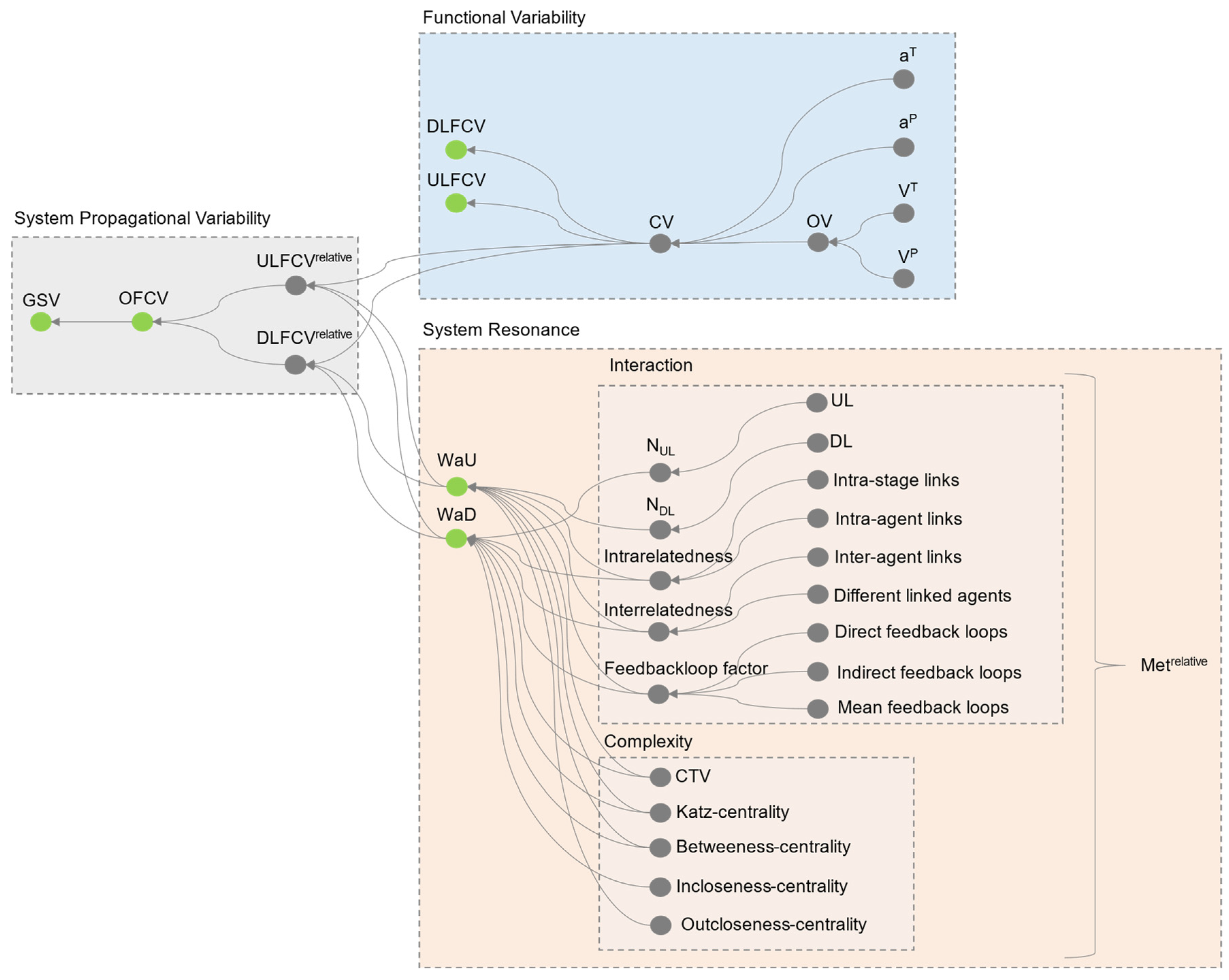
3.5. Step 3: Aggregation of Variability

The purpose of the third step is to look at how the variability of the functions aggregate and propagate through the system in a specific instantiation of the model to determine potential functional resonance leading to unexpected outcomes arising through interaction and complexity in the system. Because of the complex scenario and the fact that its qualitative modelling by FRAM was quickly becoming overwhelming, we enhanced the research by a semi-quantitative approach according to Patriarca et al. [69] and Grabbe et al. [12]. This was implemented with the help of the software myFRAM 1.0.4 [70], which was developed in Visual Basic for Applications and interfaced with Microsoft Excel and FMV, enabling the FRAM model to be converted into a matrix so that a quantitative or numerical calculation is possible. The structure of the defined metrics is shown in Figure 4. Here, the nodes represent the respective metrics, and the structure, that is which metrics are composed how, is marked by arrows and their direction from right to left. The green nodes will later be used as the main analysis metrics in Section 4.2. In general, the metrics can be divided into three categories: functional variability, system resonance, and system propagational variability. The functional variability represents the variability that a function directly receives and transfers without considering their interaction and effect in the system sufficiently. Therefore, the system resonance tries to reflect the interaction and complexity of a function in the system, incorporating non-linearity, emergence, and dynamic of the system. It is a kind of weighting of the impact and affectedness of a function to evaluate the effect of a function variability system-wide. Combining functional variability and system resonance results in system propagational variability, which shows the systemwide impact and affectedness of each function’s variability up to a global system variability level. The definition and calculation of each metric within the three categories, which were implemented with myFRAM and MATLAB 2020, are described below.

3.5.1. Metrics for Functional Variability

The final calculation of functional variability is based on the downlink (DL) and uplink (UL) coupling variability (CV) of one foreground function (downlink functional coupling variability DLFCV and uplink functional coupling variability ULFCV). The DLFCV was used to understand the implications of the coupling variabilities of one entire upstream function j to associated downstream functions i and the ULFCV was used to comprehend the impact of the variability of a downstream function i through its incoming coupling variabilities of upstream functions j. The calculation formula for DLFCV and ULFCV can be seen in (1) and (2), respectively:

$$DLFC{V}_j={\sum }_{i=1}^{j}C{V}_{ij}$$

(1)

$$ULFC{V}_{i }={\sum }_{i=1}^{j}C{V}_{ij}$$

(2)

To keep the paper readable, the formulas of the remaining metrics on which the DLFCV and ULFCV are based can be found in Appendix A.

3.5.2. Metrics for System Resonance

The performance of the overall system, in this case the FRAM model, is more than the sum of its function’s variabilities, and rather is determined by the interaction and fit of the individual subsystems (within and between agents as well as between agents and the environment). However, the metrics mentioned above did not adequately represent this and are only considered as taken separately without interactions (except for the variability propagation factors). Therefore, we further defined several metrics, categorised into an interaction and complexity dimension, which should represent this inherent complexity, which incorporates non-linearity, emergence, and dynamic of the system. On the one hand, the connectivity/interaction of functions was determined with the following metrics in order to calculate the degree to which a function interacts with other functions or agents in the system:

• Number of downlinks and uplinks ($N_{DL}$ and $N_{UL}$) which show how many functions a function can directly influence and how many functions it is directly influenced by, respectively.
• Intrarelatedness expresses how many functions a function is linked to within an agent (e.g., EV) and within the same stage (e.g., Follow) or in different stages (e.g., Follow and Pass).
• Interrelatedness presents how many functions of other agents (e.g., LV and OV) a function is linked to and weights it with the number of different agents.
• Feedback loop factor reflects the extent to which a function’s output can influence its input through direct and indirect feedback loops.

On the other hand, centrality measures from graph theory were used to represent the complexity of the system. The reason for this choice is that graph theory proved to be well suited to investigate some emergent non-linear characteristics of systems to express by other approaches and their used metrics have been already proven to succeed in explaining many features of complexity [71]. The translation of a FRAM model into a network by graph theory was already applied by Bellini et al. [72] and Falegnami et al. [71], showing general good integrability of these approaches to prioritise key functions in a FRAM model adopting centrality measures in order to reflect a combination of couplings’ weights and connectivity. However, the studies also implied that several centrality indices, representing the importance of a node/function, exist and that it is difficult for a centrality measure to be considered the most representative of FRAM characteristics since peripheral nodes/functions can also be important. Thus, the most appropriate centrality measures should be identified on a case-by-case basis [73]. Therefore, the authors of this paper chose a mix of the following three different centrality indices and one own defined metric, assuming this would be the best way to represent this complexity:

• Katz-centrality depicts the relative degree of influence of a function within the system, showing the extent of indirect impact.
• Incloseness- and Outcloseness-centrality measure how central a function is located in a system and thus the more central a function is, the closer it is to all other functions and therefore has a high potential for functional resonance.
• Betweenness-centrality shows the degree of a function to bridge functions with other functions, which makes it a critical function for system success.
• Clustered Variability (CTV) shows how much upstream and downstream variability accumulates around a function to depict where groups of functions with high variabilities exist that are directly coupled.

To keep the paper readable, the formulas of the metrics for the interaction and complexity dimensions can be found in Appendix B. Below the calculation and meaning of the two main indicators of system resonance, the Weight as Upstream (WaU) and Weight as Downstream (WaD) of a function f, are explained. The WaU and WaD reflect the system effect of a function as an upstream and downstream function, respectively. This should simulate the interaction and fit between functions and their inherent complex interdependencies. The respective metrics are included in the calculation in a weighted manner. The assignment of these weighting factors with numerical values was subjective and is reflected in

Table 3. Allocation of numerical values of the weighting factors for the calculation of WaU and WaD.

Weighting Factor	Numerical Score
${\beta }_1 (N_{DL}/N_{UL}$)	4
${\beta }_2 (Intrarelatedness$)	2
${\beta }_3 (Interrelatedness$)	2.5
${\beta }_4 (FeedbackLoopFactor$)	1
${\beta }_5 (CTV$)	1
${\beta }_6 (Katz-centrality$)	4
${\beta }_7 (In-/Outclosenness-centrality$)	2.5
${\beta }_8 (Betweeness-centrality$)	2.5

. The assignment follows the logic that some metrics weigh more heavily than others. For example, interrelatedness weighs more heavily than intrarelatedness, since this considers that influencing other agents has a higher system effect than only influencing one’s own agent. The WaU and WaD are determined as follows (3) and (4):

$$\begin{array}{cc}Wa{U}_f& ={\beta }_1\ast {N_{DL}^{relative}}_f+{\beta }_2\ast Intrarelatednes{s}_f^{relative}+ {\beta }_3\ast Interrelatednes{s}_f^{relative}+{\beta }_4\hfill \\ & \ast FeedackLoopFacto{r}_f^{relative} +{\beta }_5\ast CT{V}_f^{relative}+{\beta }_6\ast Katz-centralit{y}_f^{relative}+{\beta }_7\hfill \\ & \ast Outcloseness-centralit{y}_f^{relative}+{\beta }_8\ast Betweenness-centralit{y}_f^{relative}\hfill \end{array}$$

(3)

$$\begin{array}{cc}Wa{D}_f& ={\beta }_1\ast {N_{UL}^{relative}}_f+{\beta }_2\ast Intrarelatednes{s}_f^{relative}+ {\beta }_3\ast Interrelatednes{s}_f^{relative}+{\beta }_4\hfill \\ & \ast FeedackLoopFacto{r}_f^{relative} +{\beta }_5\ast CT{V}_f^{relative}+{\beta }_6\ast Katz-centralit{y}_f^{relative}+{\beta }_7\hfill \\ & \ast Incloseness-centralit{y}_f^{relative}+{\beta }_8\ast Betweenness-centralit{y}_f^{relative}\hfill \end{array}$$

(4)

3.5.3. Metrics for System Propagational Variability

In the final step, the WaU and WaD are offset against the CV values of each function, resulting in a relative DLFCV (5) and relative ULFCV (6) considering the interaction of one function’s down- and uplink coupling variability within the whole system, showing how a function affects the system and is affected by the system, respectively:

$$DLFC{V}_j^{relative}={\displaystyle \sum }_{i=1}^{j}C{V}_{ij}\ast Wa{U}_j\ast Wa{D}_i$$

(5)

$$ULFC{V}_i^{relative}={\displaystyle \sum }_{j=1}^{i}C{V}_{ij}\ast Wa{U}_j\ast Wa{D}_i$$

(6)

Finally, the overall functional coupling variability (OFCV) of a function f could be determined from this (7):

$$OFC{V}_f=ULFC{V}_i^{relative}+DLFC{V}_j^{relative}$$

(7)

This metric identifies critical functions with high potential for functional resonance offering functional prioritisation of their impact into the system in that, for example, a high value means that the function has a large systemic effect and/or is largely systemically affected and/or a high variability accumulates in and around the function.

In the last step, a global system variability (GSV) could be calculated to show the accumulated variability of all functions and their interactions of the whole system for one specific condition. This enables, for example, a comparison of system performance between a system where purely human drivers operate and one where an automated system operates with human drivers. The GSV is the sum of the OFCVs of n functions within the whole system (8):

$$GSV={\displaystyle \sum }_{f=1}^{n}OFC{V}_f$$

(8)

3.6. Step 4: Management of Variability

The final step proposes ways to manage performance variability, especially possible conditions of functional resonance, that have been found by the preceding steps. In this work, we proceeded as follows. In general, we are aiming to improve the performance variability of the entire system for the given scenario by deriving system design recommendations through a well-reasoned function allocation, which will be shown in Section 4.3. To achieve this, the performance variability of the entire system is analysed by comparing the contributions between human driver and automation to road safety based on systemic mechanisms on both an abstract global level (see Section 4.2.1 and Section 4.2.2) and a fine grain level regarding the individual functions (see Section 4.2.3 and Section 4.2.4).

4. Results

In this section, the results are presented. First, the resulting overall FRAM model is described. Further, critical functions are identified and analysed in-depth to compare the positive and negative contributions of the human driver and automation to system behaviour. Finally, recommendations for system design as well as the validation process of AD are derived.

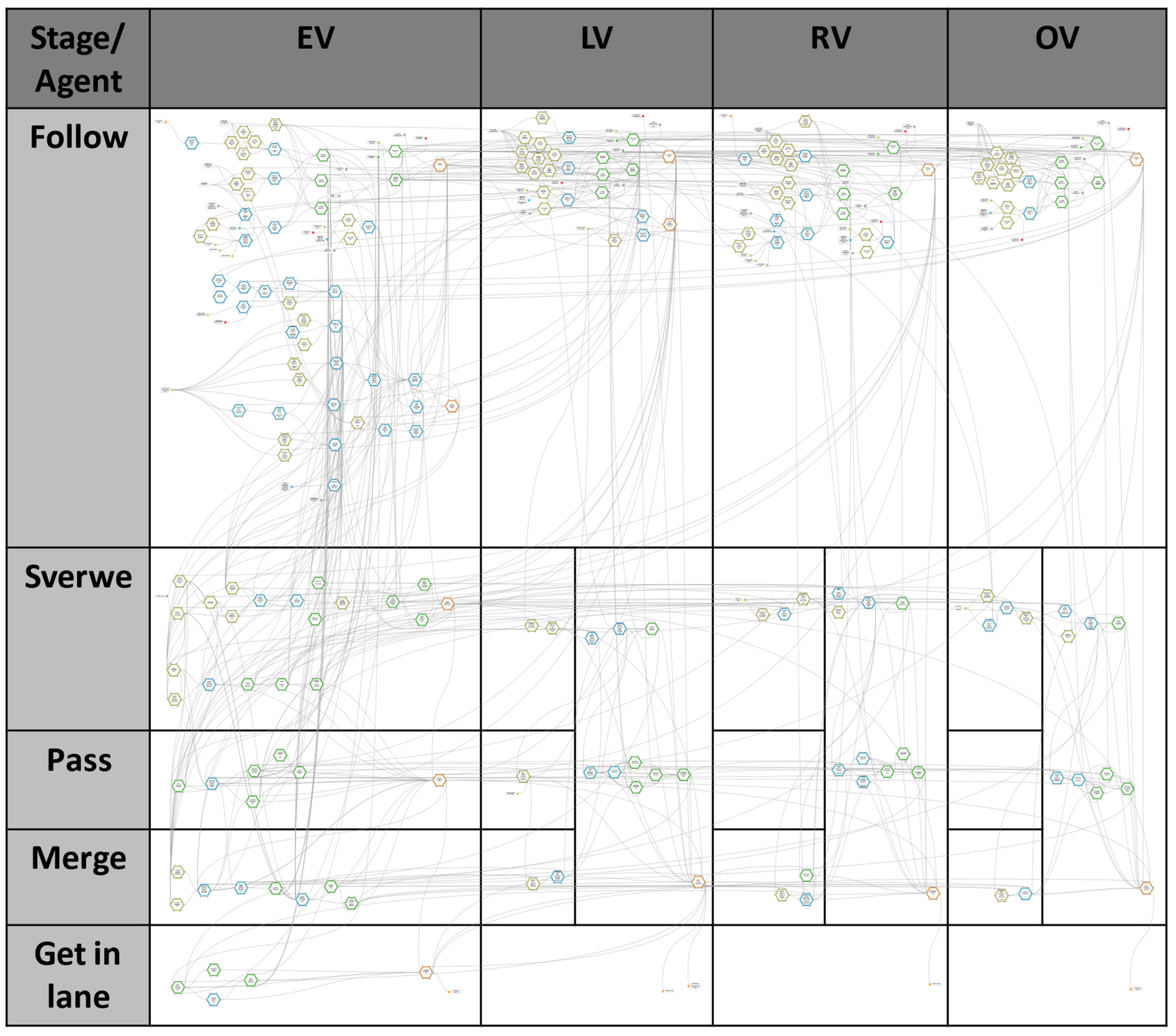
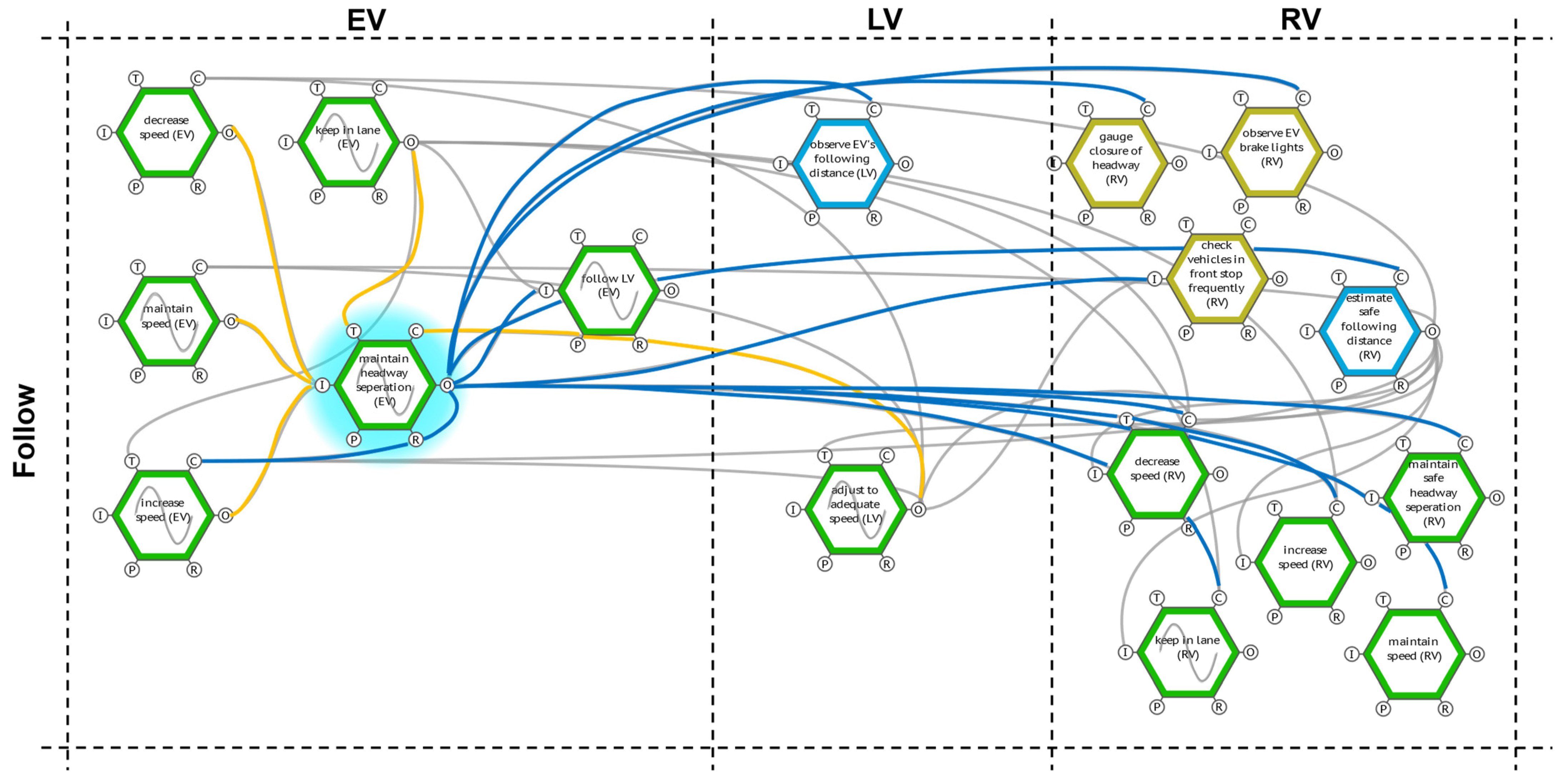
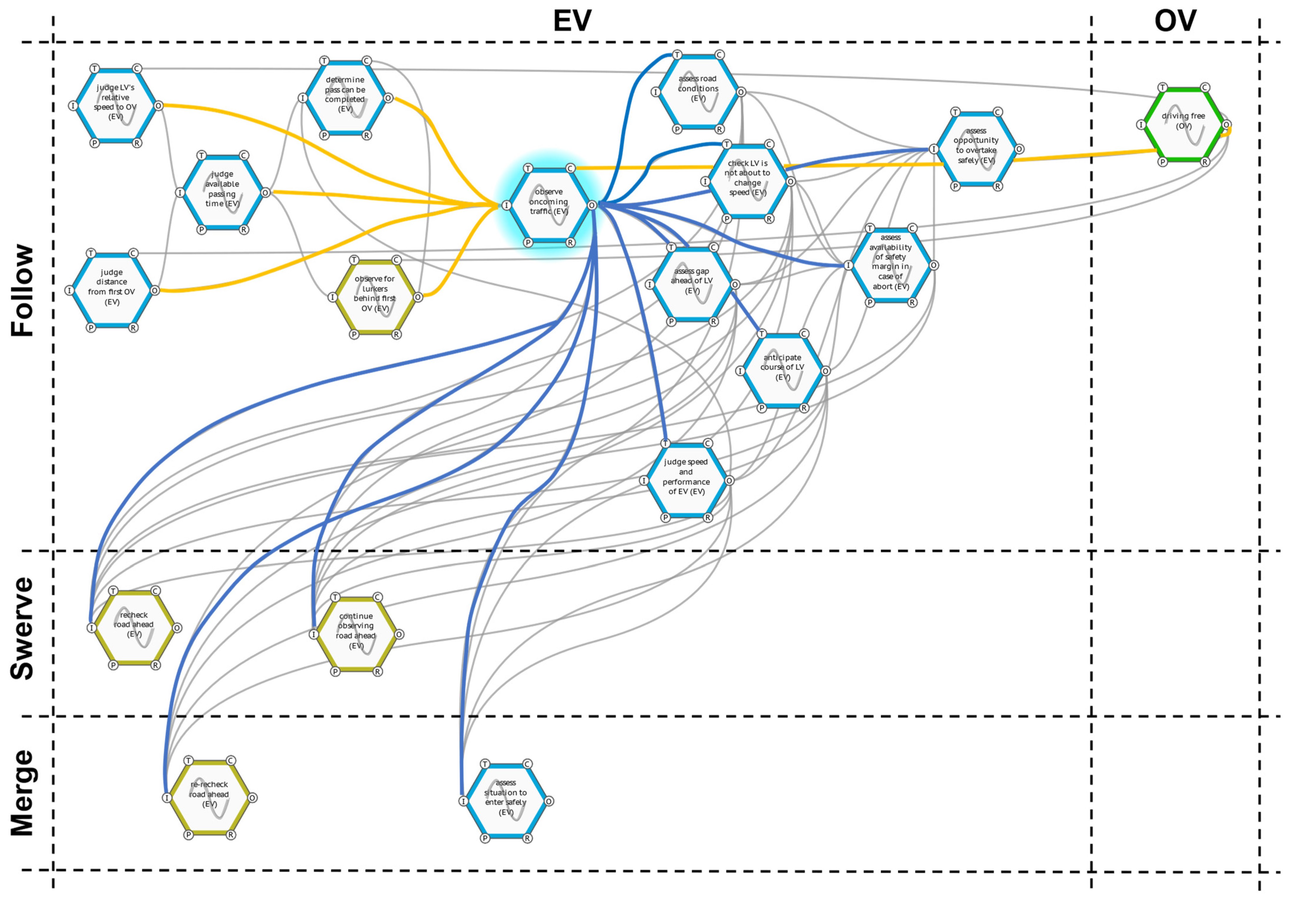
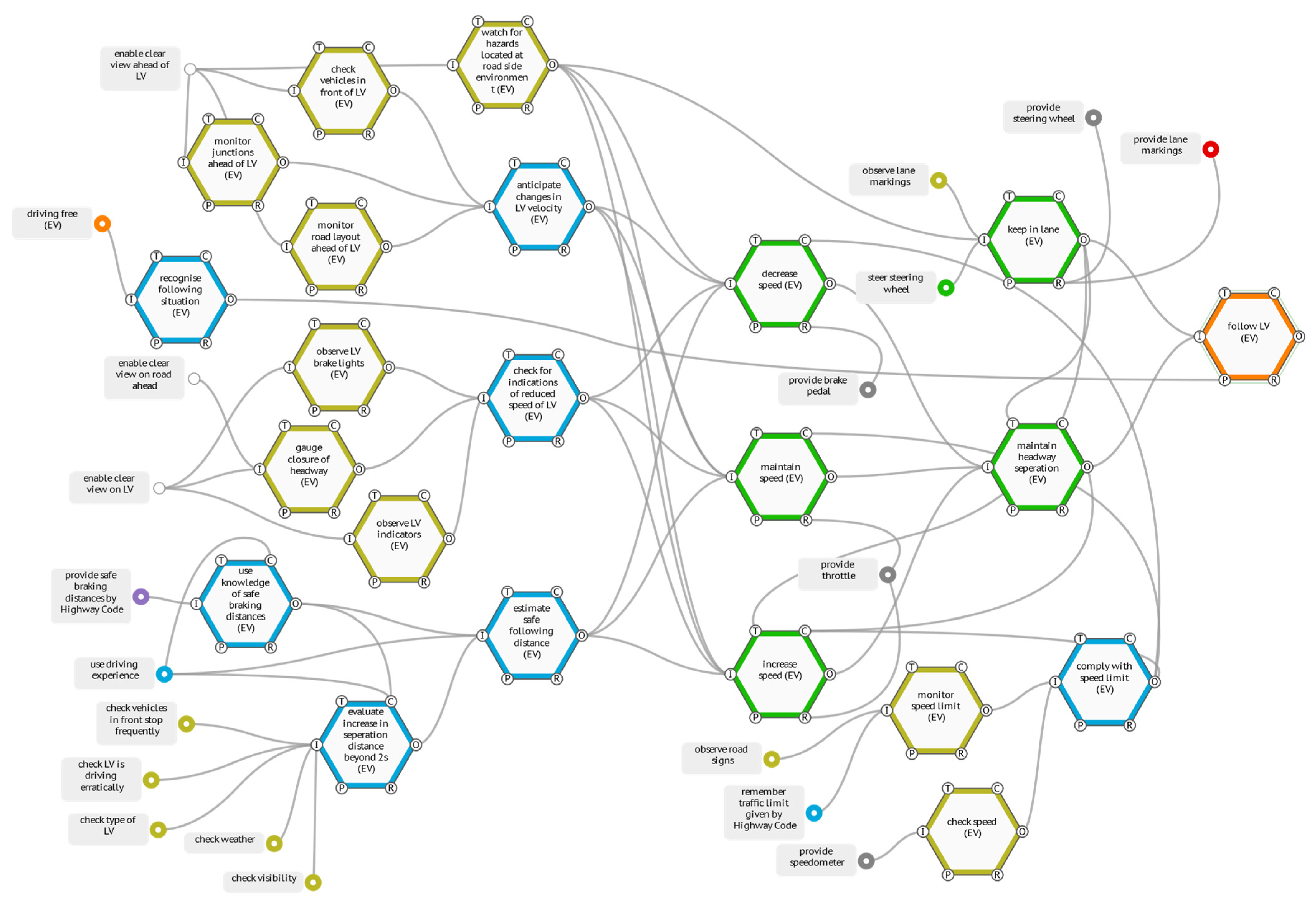
4.1. The Overall FRAM Model

The overall model comprises 285 functions (210 foreground functions (hexagons) and 75 background functions (rectangles)) with 799 couplings and is shown graphically in Figure 5. All functions within an agent exist only once and are then executed several times by other functions at different stages of the manoeuvre. The functions are assigned respectively to the four different agents (EV, LV, RV, and OV) and five temporal stages during the scenario (Follow, Swerve, Pass, Merge and Get in lane). This is a modification of the Abstraction/Agency framework by Patriarca et al. [74] into a Space-Time/Agency framework, which should ensure enhanced knowledge representation combined with a multi-dimensional approach that is two dimensions: the temporal-spatial levels and the agency levels. Since it is not effective to analyse an STS according to only one level [74], this approach makes it easier to with complexity that requires a system to be structured following different levels of analysis with different resolutions and perspectives [75]. This is shown by the interactions within an agent and between different agents at different temporal and spatial occurrences. The stages always refer to the perspective of the EV, which is the focus of analysis. The functions can only be executed within the assigned agent and the assigned temporal stage(s) but can be coupled with functions of all other agents and stages.

To make the model clearer, the functions have also been colour-coded according to the following pattern to specify the type of functions in more detail:

• Driving functions:

  ○

  Yellow → perception driving tasks (e.g., to monitor road layout ahead of LV)

  ○

  Blue → cognition driving tasks (e.g., to assess the opportunity to overtake safely)

  ○

  Green → action driving tasks (e.g., to decrease speed)

  ○

  Orange → main manoeuvre tasks (e.g., to follow LV)

• Functions affecting driving:

  ○

  Red → characteristics of the infrastructure (e.g., to provide road signs)

  ○

  White → characteristics of the environment (e.g., to enable clear view on the road ahead (weather conditions, etc.)

  ○

  Grey → technical functions of the vehicle (e.g., to provide steering wheel)

  ○

  Purple → information by the policy (e.g., to provide safe braking distances by Highway Code)

The driving functions are classified into three levels of information processing (i.e., perception, cognition, and action) adopting the framework of types and levels of automation regarding the four-stage model of human information processing provided by Parasuraman et al. [76]. This facilitates function allocation between humans and automation, that is, the design decision of which system functions are to be performed by humans and which should be automated and to what extent to improve system safety. Thereby, main manoeuvre functions bundle several driving functions, which are intended to improve clarity.

It should be noted that the model is the same for the human driver or the automation because of the assumption that there is no change in the functions of the system that have to be accomplished by the human driver or the automation. This is ensured by an appropriate resolution or abstraction of the functions. The difference between the two agents is only the variable performance of each function. The reason is that a FRAM model should treat humans and automation systems as equivalent producers of functions to compare the joint performance of both systems as the net result of the functional resonances as depicted by the GSV.

Due to the complexity of the model, we cannot represent and describe the actual structure and content of the whole model (the entire model can be viewed as an FMV data file in the Supplementary Materials S1). Therefore, we roughly describe the major functions per each agent and stage represented by the main manoeuvre functions in Appendix C in

Table A3. A rough description of the main functions of the overall FRAM model per each agent and stage.

Stage	EV	LV	RV	OV
Follow	to follow LV through recognising the following situation, keeping the lane, and maintaining headway separation; to decide to overtake or not, which is mainly based on assessing the opportunity to overtake safely, judging whether overtaking is permitted, and evaluating the reasonableness for overtaking	to drive free by keeping the lane and adjusting adequate speed; to react to being followed by EV through observing EV’s intention to overtake as well as its following distance	to follow EV through recognising the following situation, keeping the lane, and maintaining headway separation	to drive free by keeping the lane and adjusting adequate speed
Swerve	to adopt the overtaking position by lane keeping, reducing headway from the normal following, and adjusting the speed to that of LV; to swerve completely to the oncoming lane afterwards checking any hazards behind or in front, assessing the overtaking opportunity is still safe and using the left indicator	to detect EV’s swerving into the oncoming lane; to maintain speed; to react to being passed by responding to potential passing problems of EV (optional)	to detect EV’s swerving into the oncoming lane; to react to being passed by responding to potential passing problems of EV (optional)	to detect EV’s swerving into the oncoming lane; to maintain speed; to react to being passed by responding to potential passing problems of EV (optional)
Pass	to perform the overtaking through accelerating LV decisively or merging back into starting lane if the manoeuvre is unsafe and abandoning the manoeuvre	to detect the passing vehicle in peripheral vision; to react to being passed by responding to potential passing problems of EV (optional)	to react to being passed by responding to potential passing problems of EV (optional)	to react to being passed by responding to potential passing problems of EV (optional)
Merge	to merge progressively into the starting lane by adjusting EV’s speed in relation to other traffic, assessing the situation to enter safely, and using the right indicator	to prepare to provide a larger opening for EV to merge back; to react to being passed by responding to potential passing problems of EV (optional)	to prepare to provide larger space to LV in case of EV’s manoeuvre abandoning or to catch up to LV; to react to being passed by responding to potential passing problems of EV (optional)	to prepare for braking; to react to being passed by responding to potential passing problems of EV (optional)
Get in lane	to complete the overtaking through positioning into the starting lane evaluating the driving situation, and resuming at the desired speed	to follow EV; to react to being followed by RV	to follow LV	to drive free

The wording “(optional)” means that this function or task is not necessarily fixed to the assigned stage and rather can be executed in the Swerve, Pass, or Merge stage or not at all if not required.

. Additionally, the driving behaviour of to follow by EV in the Follow stage (see Appendix C in Figure A1) is explained in detail to improve the comprehension of the remaining parts of the model.

4.2. Comparison of the Contributions between Human Driver and Automation to Road Safety Based on Systemic Mechanisms

In this subsection, the analysis process follows the hierarchical structure of the metrics depicted in Figure 4, moving from the abstract (left) to the detailed (right) focussing primarily on the main analysis metrics (green nodes). First, the abstract global analysis is accomplished through prioritising risk functions and analysing them in comparison across stages and function types between human driver and automation. Additionally, the global system variability is investigated. Second, the individual functional analysis is represented by distinguishing the interaction and variability of system functions to identify potential critical functional resonance, but also success factors, and finally analysing critical paths and their interactions in the system.

In general, a comparison of all system functions cannot be presented, so the following is an analysis of essential functions serving as examples to assist with comprehension of the derivation of system design recommendations in Section 4.3.

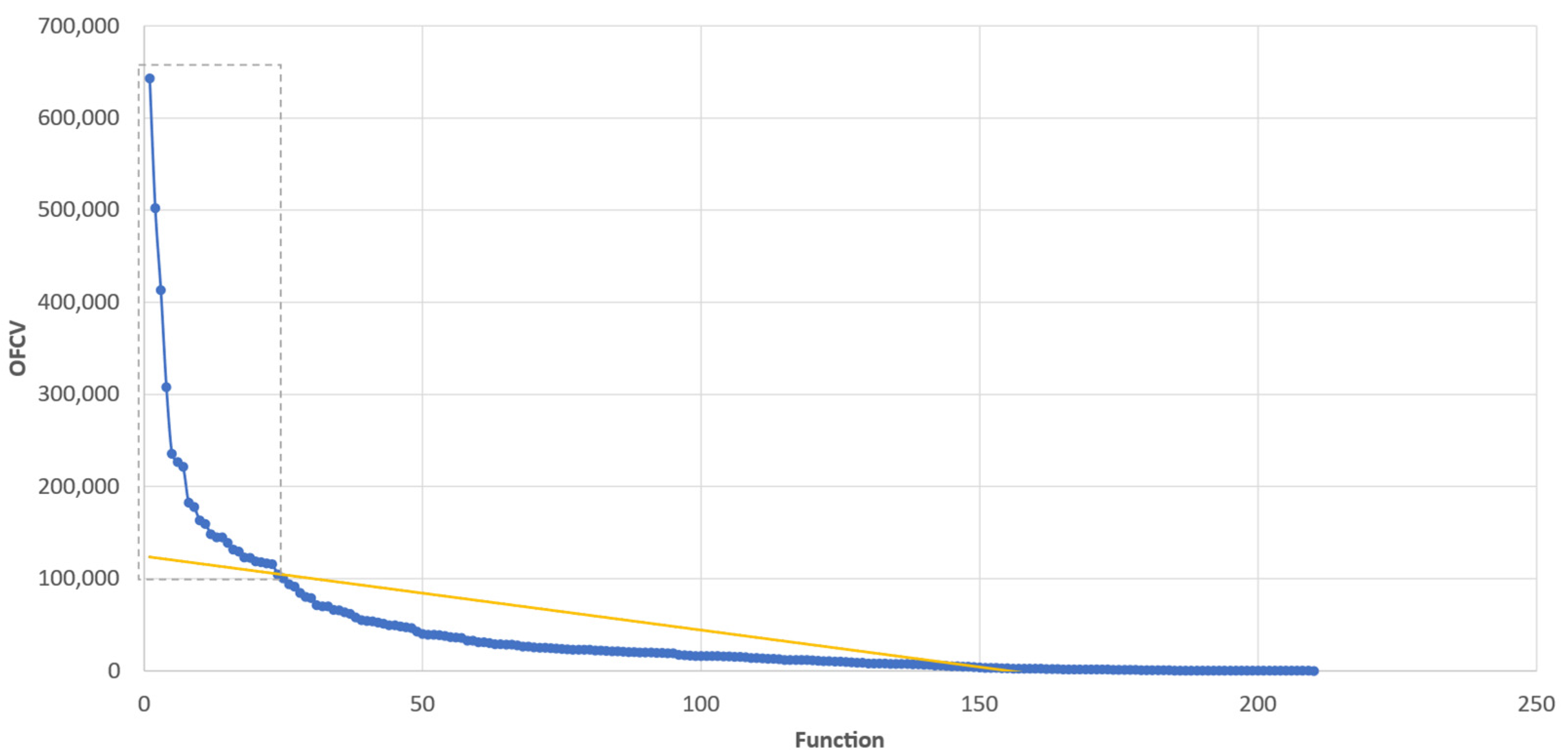
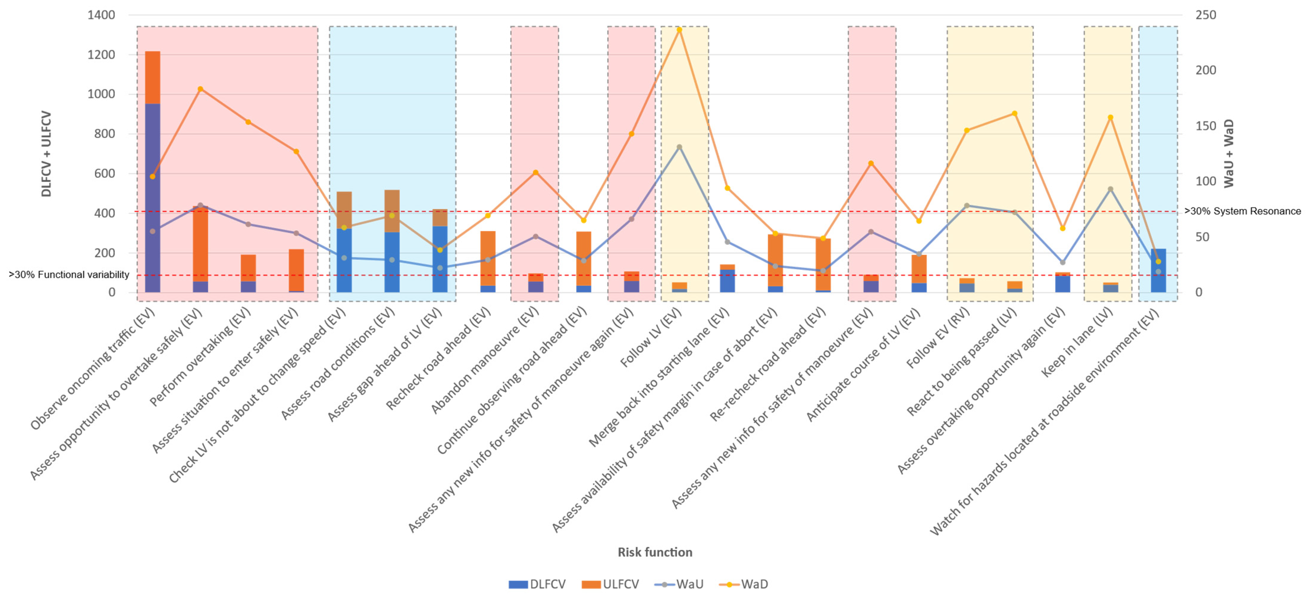
4.2.1. Prioritisation and Analysis of Risk Functions

The risk functions for human drivers and automation were identified through the analysis of the OFCV since this metric shows the criticality of a function measured by the system-wide impact of the function’s variability. Here, the OFCV of each function was prioritised and ranked using the scree test (see Figure 6) according to Falegnami et al. [71]. Usually, the first knee is chosen to prioritise functions that lie left to the curve knee (that in our case filters only five functions, which are largely more critical than the following ones). However, as we are interested in focusing on a larger portion of risk functions, we needed a tool to help us decide which curve knee to use. Thus, we enhanced the scree test by a regression line. The rightmost curve knee, which lies above the first intersection point of the regression line (i.e., functions that lie above the average linear slope and thus differ significantly from functions below the average linear slope), is ultimately used as the decision criterion. Thus, we selected the third knee, allowing us to consider 23 risk functions for the human driver. The selection process for the automation was the same, resulting in 22 risk functions. A list of risk functions is shown in Appendix D in

Table A4. Risk functions for human driver and automation.

Risk Function	Human	Automation
Follow LV (EV)	x	x
Maintain headway separation (EV)	x
Perform overtaking (EV)	x	x
Assess opportunity to overtake safely (EV)	x	x
Check LV is not about to change speed (EV)		x
Follow EV (RV)	x	x
React to being passed (LV)	x	x
Assess road conditions (EV)		x
Adopt overtaking position (EV)	x
Assess gap ahead of LV (EV)		x
Driving free (OV)	x
Keep in lane (LV)	x	x
Keep in lane (EV)	x
Recheck road ahead (EV)		x
Abandon manoeuvre (EV)		x
Assess any new info for safety of manoeuvre again (EV)	x	x
Respond to EV’s passing problems (LV)	x
Adjust to adequate speed (LV)	x
Respond to EV’s passing problems (RV)	x
Merge back into starting lane (EV)	x	x
Assess situation to enter safely (EV)	x	x
Continue observing road ahead (EV)		x
Driving free (LV)	x
Keep in lane (OV)	x
Respond to EV’s passing problems (OV)	x
Assess availability of safety margin in case of abort (EV)		x
Re-recheck road ahead (EV)		x
React to EV’s overtaking (RV)	x
Anticipate course of LV (EV)		x
Recognise that EV is experiencing problems passing (LV)	x
Increase speed (EV)	x
Assess overtaking opportunity again (EV)		x
Assess any new info for safety of manoeuvre (EV)	x	x
Watch for hazards located at roadside environment (EV)		x

. The risk functions are not only related to the agent EV, but also the other agents. Considering a function allocation for the system design (which will be explained in more detail in Section 4.3.1), the following should be taken into account. If a function is only an automation risk, it is recommended that it should be performed by humans, and vice versa. However, if a function poses a risk to both, it is necessary to analyse thoroughly which control mode seems to be the best.

As seen in Figure 7, the most risk functions are in the Follow stage, which also includes significantly more functions, however. In the other stages, the distribution is about the same, except for the Swerve/pass/merge stage, in which humans have six times more risk functions than automation. However, the risk functions in this stage are all performed by other agents than EV, so it can be interpreted that the other agents are more negatively influenced by the human driver of EV than by the automation. However, this would need to be verified since the other agents are only influenced by action functions and these are predominantly performed worse by the human. Furthermore, the data from other agents are only based on experiences with human drivers and not with automation. Moreover, the Get in lane stage is the only stage without a risk function.

Figure 8 shows that the risk functions for automation are mainly loaded by perception and cognition. Merely one third relates to action and main manoeuvre functions. In humans, on the other hand, mainly action functions and the main manoeuvre functions are considered risk functions, whereby the main manoeuvre functions are predominantly action-intensive. Only one fifth is accounted for by cognition functions, and perceptual functions do not pose any risks at all.

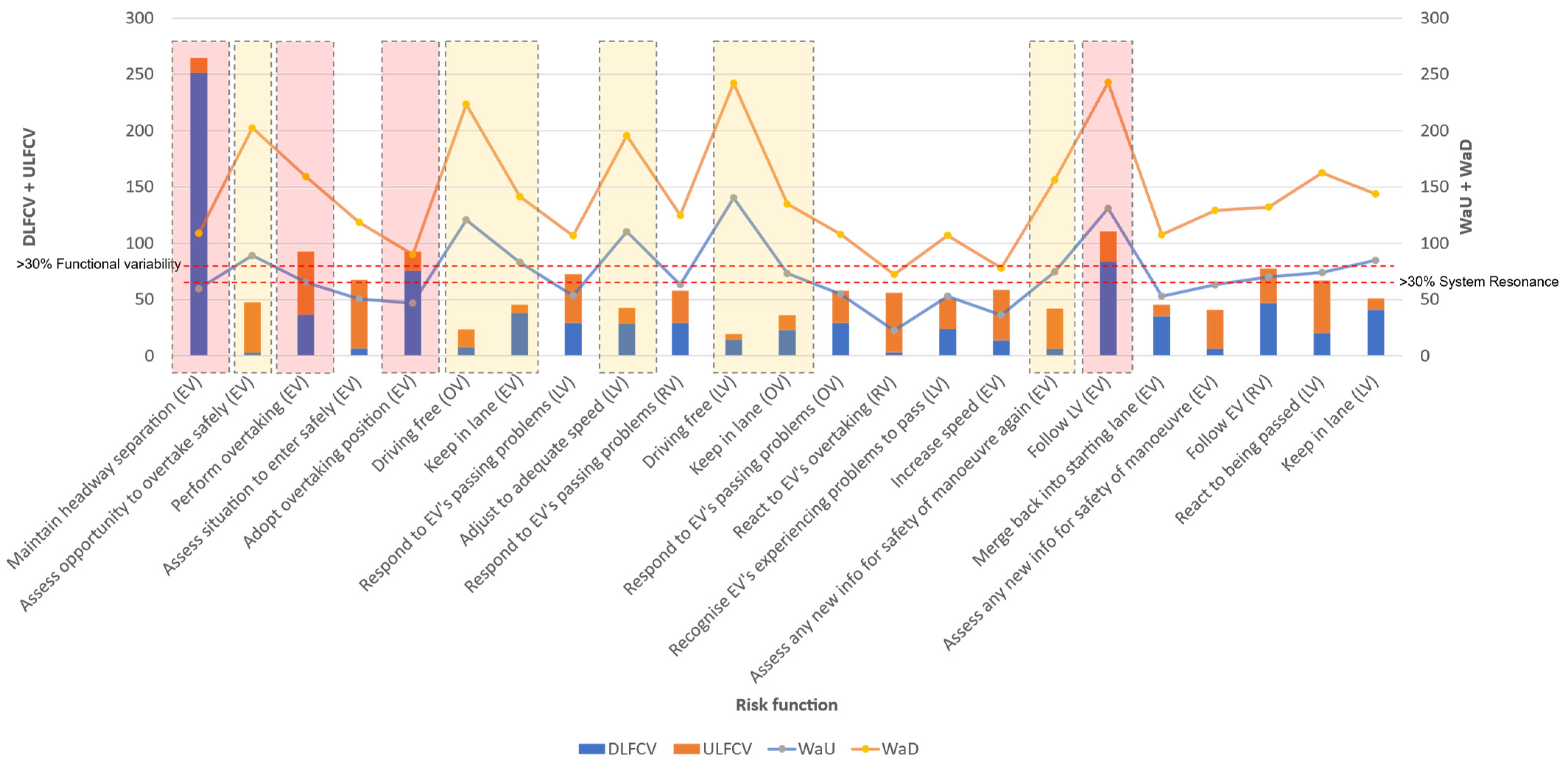
4.2.2. Analysis of Global System Variability

Finally, the GSV of each stage between human and automation is compared, as well as the function types for the EV in each stage. Figure 9 shows the comparison of GSV between humans and automation, where the variability is calculated in relation to the number of functions in the stage so that they can be compared relatively. The highest variability for both is found in the Pass stage and the largest difference between humans and automation occurs in the Follow stage, where the automation’s variability is much larger than for humans. The other stages are relatively balanced, although the variability in automation is slightly lower. In general, automation has a higher overall variability.

4.2.3. Distinguishing the Interaction and Variability of System Functions for Potential Critical Functional Resonance

The previous analysis was very focused on the OFCV of risk functions and the GSV, which reflect the criticality of the functional variabilities in the system in an aggregated, abstract and simplified form. However, this criticality is composed of two dimensions: the variability a function receives (ULFCV) and transfers (DLFCV), which represent the functional variability, and the system resonance of a function, which reflects the interaction in the system, is how the functional variability is affected by the system (WaD) and how it influences the system itself (WaU). Therefore, these two dimensions were analysed separately for the system functions as well as risk functions in the following to get a deeper understanding. This is proposed by a matrix that represents the criticality of functions and their potential for functional resonance along the two dimensions functional variability and system resonance, which make up Functional Variability-System Resonance Matrix (FVSRM) (see Figure 10), a modification of the Variability Impact Matrix presented by Patriarca et al. [45]. For each function, the FVSRM considers in the system resonance dimension the sum of the WaU and WaD: low system resonance if it is lower than 5% of the maximum of the sum of WaU and WaD, medium system resonance if it is between 5%-30% of the maximum, and high system resonance if it is higher than 30% of the maximum. The functional variability dimension is considered by the sum of the DLFCV and ULFCV, where the three thresholds are analogous to the first dimension. The thresholds for both dimensions were determined subjectively by SMEs, inspired by the procedure of Patriarca et al. [45].

The FVSRM shows different areas: green (C-C, C-B, B-C) for uncritical functions, blue (A-C) for high variable functions with low system resonance, yellow (B-B) for medium variable functions with medium system resonance that are between uncritical and critical functions, orange (C-A) for low variable functions with high system resonance and red (B-A, A-A, A-B) for critical functions. Here, the orange and blue areas refer to functions that must be viewed with caution due to their special features. Functions in the blue area are functions that are typically error-prone but usually remain without adverse consequences (i.e., accidents) because they have a low systemic resonance. Functions in the orange area are functions where errors rarely occur, but when they happen, a strong systemic effect and consequently a high probability of accidents must be expected. In general, the functions in the orange area pose a greater hazard than the blue ones and are thus to be assessed as more critical. Below the FVSRM, the sum of functions per area is presented. Furthermore, the sum of functions per row and column is given to reflect the number of functions per dimension category.

The distribution of the functions in the FVSRM in Figure 10 shows that the system for the human driver is generally stable in terms of variability as five functions are above 30% functional variability but is affected by several interrelated functions with great system resonance impacts as 40 functions are above 30% system resonance. Instead, the distribution of the functions in the FVSRM for the automation is significantly more unstable in terms of variability as 25 functions have a functional variability of greater than 30%. Overall, the automation shows higher variable and medium system resonance functions. The number of uncritical functions is nearly the same for both at about 40%, with critical functions outweighing humans (19%) for automation (26%).

The risk functions for human drivers and automation were also analysed in a more differentiated way concerning the two dimensions of functional variability and system resonance, see Figure 11 and Figure 12. Figure 11 shows the functional variability (DLFCV and ULFCV as stacked columns, left y-axis) and system resonance (WaU and WaD as stacked line markers, right y-axis) of risk functions (x-axis) for the human driver and Figure 12 for automation. Additionally, the thresholds for high functional variability and high system resonance are marked by the two dashed red lines. Some risk functions for the human driver are highlighted and explained below. The red highlighted functions are most critical because they have a high functional variability combined with high system resonance. Here, < maintain headway separation (EV) > and < follow LV (EV) >, in particular, stand out, with high variability and system resonance values, whereby they transfer variability for the most part and receive very little. In addition, each critical risk function is an action task. The orange highlighted functions are risk functions that have relatively low variability but combined with a strong system resonance. It can be argued that these functions are success factors demonstrating resilience because, despite their strong system effect and affectedness, they have little variability and are therefore stable. In particular, < driving free (OV) > and < driving free (LV) > with very high system resonances are noteworthy here. These functions must nevertheless be viewed with caution, especially under different scenario conditions, as a sudden increase in variability in these functions may have a large systemic effect. The function < assess opportunity to overtake safely (EV) > is also special because it is strongly influenced by the system and receives a relatively large amount of variability, but transfers very little variability into the system. Further, the functions < assess opportunity to overtake safely (EV) > and < merge back into starting lane (EV) > exhibit fairly high system resonances, but with relatively low variability. So, errors rarely occur here, but if they do, then they often result in accidents. Risk functions, either high variability combined with low system resonance or low variability joined with low system resonance, do not exist. By contrast, the latter is logical, otherwise, they would not be considered as risk functions.

Compared to the automation in Figure 12, it can be seen that humans have significantly lower variability values and that overall, significantly more risk functions in automation have high functional variability. However, the values of the system resonance are slightly higher for the human risk functions than for automation ones.

Several risk functions are also colour-coded in the automation (see Figure 12). This results in seven critical functions (red), with < observe oncoming traffic (EV) > standing out. Conspicuous compared to the human driver is the distribution of critical functions among the function types: five cognitive tasks, one perceptual task, and only two action tasks. Furthermore, four risk functions can be identified as success factors (orange), for example < follow LV (EV) > and < keep in lane (LV) >, each with high systemic resonance and low variability. In addition, there are risk functions in automation that have a relatively low systemic impact but are highly variable (blue), especially < watch for hazards located at roadside environment (EV) > or < assess road conditions (EV) >. It can be argued that these high functional variabilities are somewhat irrelevant because of their low system resonance, and therefore, they rarely lead to adverse events. Nevertheless, this variability should not be underestimated, especially if the scenario conditions change and thus the system resonance may change.

4.2.4. Analysis of Critical Paths

The quantitative evaluations shown previously were used to obtain an overview of the influence of system functions and their variabilities and interactions in the system in comparison between human driver and automation. Finally, this information was qualitatively reflected in the model to enable the mechanisms to be fully understood. In the following, this is exemplified by one critical path each for the human driver and the automation. In this work, a critical path is defined as the direct couplings between a risk function and its upstream and downstream functions, which is why all indirect couplings are hidden, except the couplings between the direct upstream and downstream functions.

Figure 13 shows the critical path of the function < maintain headway separation (EV) >, which is highlighted in light blue and will be referred to in the following as function in focus 1 (FiF1), for the human driver with respective agents and stages. The upstream couplings are highlighted in orange and the downstream couplings in blue. Additionally, every function’s hexagon belonging to the orange or red area according to the FVSRM is marked with a sine curve indicating critical functions. Additionally, the types of functions are labelled by the respective colours, as mentioned in Section 4.1.

The FiF1 has five uplinks with little incoming variability and twelve downlinks transferring a high variability output, solely in the Follow stage. The uplinks come from four EV functions and one LV function, which are all action functions. Interestingly, four of the five upstream functions are critical, since they receive a relatively large amount of variability, which, however, is not transferred to very much. In addition, it is noticeable that < keep in lane (EV) > is temporally connected with FiF1 and thus two critical functions are executed simultaneously, inducing a potential higher workload. The downlinks go predominantly to RV (9), so RV is strongly influenced by FiF1. Otherwise, this offers great potential for resilient system behaviour, in that RV can dampen the received variability through adapted behaviour. Only one downlink goes to LV and two to EV itself, whereby a direct feedback loop between < increase speed (EV) > and FiF1 is created, so the two functions can mutually resonate. Moreover, the downlinks are predominantly associated with action functions (7) and few with perceptual (3) or cognitive functions (2). In general, the FiF1 has low intrarelatedness but high interrelatedness (3rd highest); in particular, the upstream function < keep in lane (EV) > and downstream function < follow LV (EV) > also have very high interrelatedness, so they form a “strongly interacting function triangle” here. It can be said that overall, the critical path of FiF1 is very action-heavy, has high interaction with other agents, a lot of variability accumulates in and around FiF1 (due to high CTV), and FiF1 has a strong system effect but is relatively little affected.

Figure 14 depicts the critical path of the function < observe oncoming traffic (EV) >, which is highlighted in light blue and will be referred to in the following as function in focus 2 (FiF2), for the automation with respective agents and stages. The FiF2 has six uplinks with high incoming variability and eleven downlinks transferring a high variability output, mostly in the Follow stage and less in the swerve and merge stages. The uplinks come from five EV functions and one OV function, which are four cognitive functions, one perception, and one action function. Interestingly, the distribution of upstream variability is very different with 60% coming from < determine pass can be completed (EV) > and < observe for lurkers behind OV (EV) > (30% each), and the rest coming from < judge available passing time (EV) > (18%), < judge LV’s relative speed to OV (EV) > (11%), < judge distance from first OV (EV) > (10%), and < driving free (OV) > (1%). The downlinks go merely to EV’s functions and predominantly to the Follow stage (7), only two downlinks go to each of the swerve and merge stages. In particular, the FiF2 is temporally coupled with five downstream functions, that is < assess road conditions (EV) >, < check LV is not about to change speed (EV) >, < assess gap ahead of LV (EV) >, < anticipate course of LV (EV) >, and < judge speed and performance of EV (EV) >, and thus six functions are executed simultaneously. In particular, most of these downstream functions also have a highly variable output and they are all received as an input in < assess opportunity to overtake safely (EV) >, which in total offers great potential for functional resonance. Moreover, the downlinks are predominantly associated with cognition functions (8) and few with perceptual functions (3). In general, the FiF2 is mainly connected to critical functions (except two functions) with high intrarelatedness but low interrelatedness. It can be said that overall, the critical path of FiF2 is very cognition- and perception-heavy, has high interaction within an agent over different stages, a lot of variability accumulates in and around FiF2 (due to high CTV), and FiF2 has a strong system effect and also high system affectedness, making it a highly critical function within EV’s operations by automation.

4.3. Recommendations for System Design and Validation

Based on the previous analyses, this subsection deals with recommendations for system design concerning the EV functions to improve the safety of the overall traffic system, as well as for validation focus of automation to reduce the test effort. First, a function allocation between human driver and automation is presented, followed by recommendations for automation’s validation process.

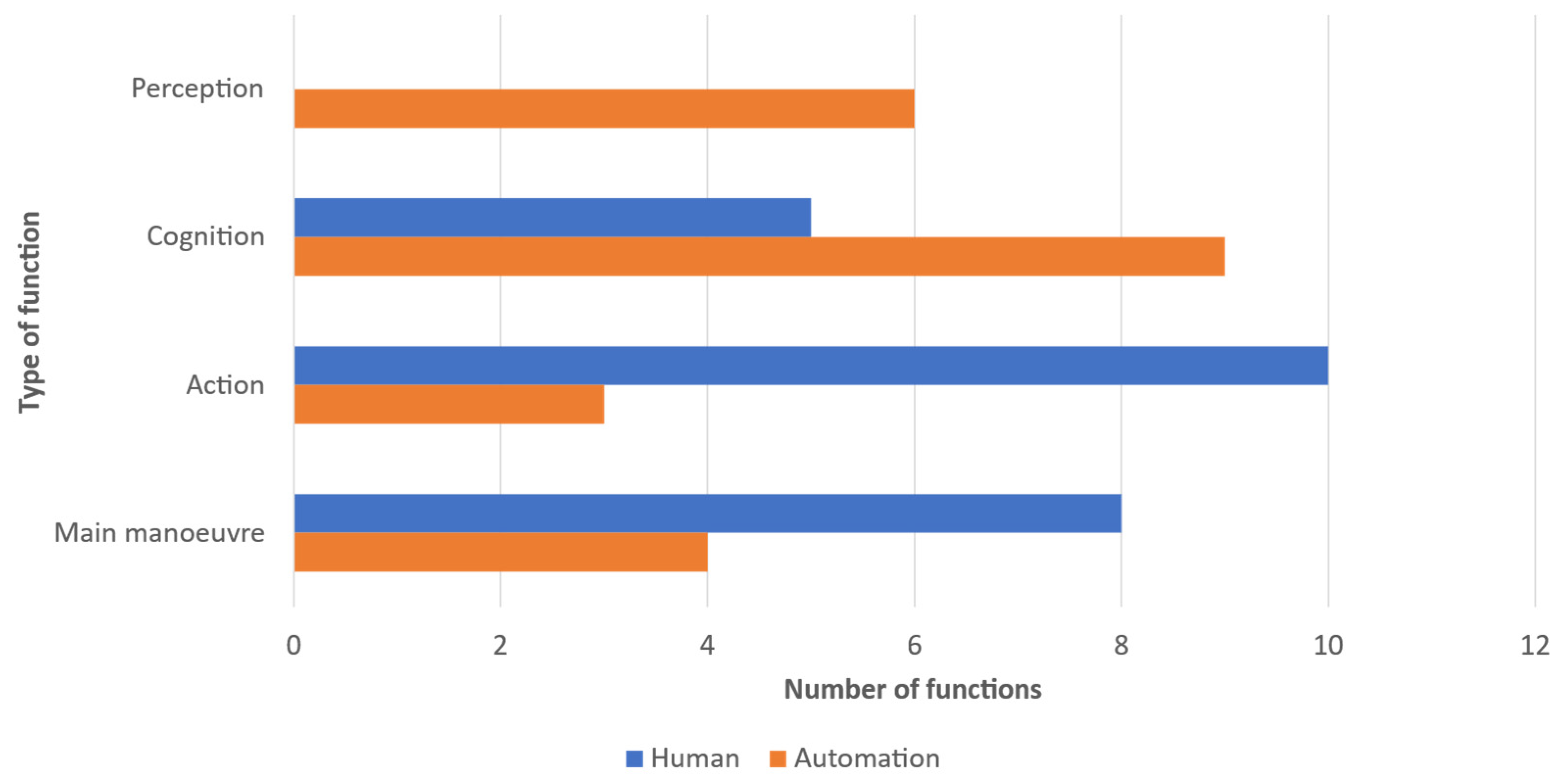
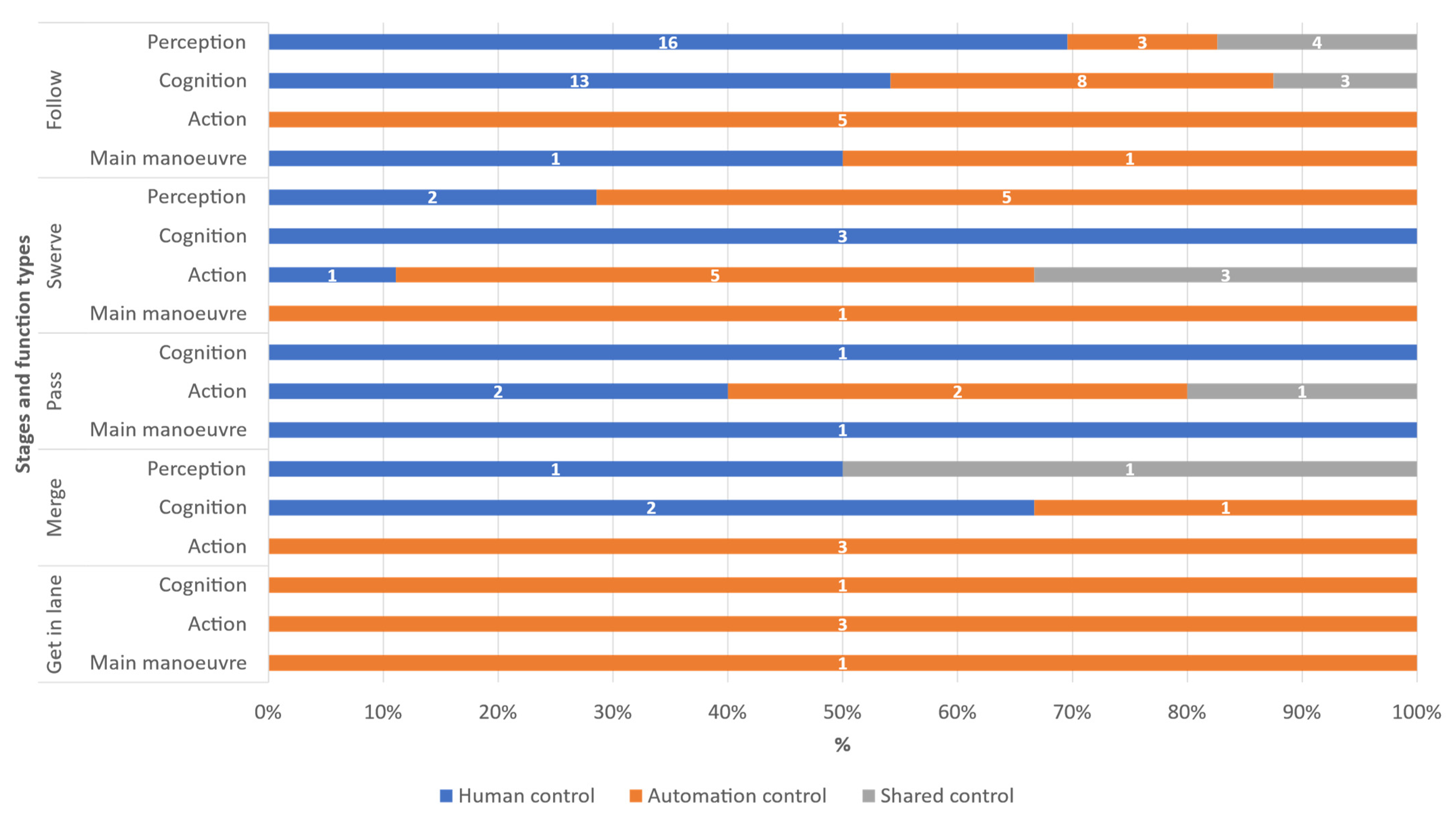
4.3.1. Function Allocation between Human Driver and Automation

Automation of the entire scenario is not recommended, as automation is significantly more variable than humans in global system variability. However, the individual stages where automation is less variable could be automated in the sense of an authority transfer. The Follow and Pass stages would then be carried out by humans, and the Swerve, Merge and Get in lane stages by automation. With this approach, however, the individual functions are not considered and the automation of certain functions per stage would represent a more differentiated approach based on the compensatory design principle for automation according to Fitts [77], see Figure 15. Here, the function allocation for EV between humans and automation is shown. The driving tasks are divided according to stages and function types within the stages. The driving tasks are performed by the human (blue), by the automation (orange), or by both in the sense of shared control (grey), which is depicted both as a percentage and as an absolute value. In this paper, shared control means that the human and the automation work in collaboration simultaneously to achieve a single function [78] as an extension, that is, the capabilities of the human are extended by the automation or vice versa [79].

The decision about the assignment of the functions is based on the previous quantitative as well as qualitative analyses and the comparison of the functional variability and system resonance of each EV’s function between humans and automation. If there was no clear and significant difference regarding the main performance indicators in a specific function between the human and automation, further metrics from Section 3.5, as well as the interaction with other functions and their performance indicators (see Section 4.2.4), were used.

First of all, it is noticeable that in the Follow and Pass stage, most of the functions are executed by humans and in the other three stages, the majority are executed by automation. The last stage in particular is performed exclusively by automation. Only 12% of all functions are executed as shared control, whereby this can take place at all three information processing levels. With the types of function, it is noticeable that humans perform significantly more perception and cognitive functions than automation, except in the Swerve or Get in lane stage, respectively. Action functions, on the other hand, are carried out significantly more by automation. Two of the five main manoeuvre functions should primarily be carried out by the human driver. These are the decision to overtake and the overtaking manoeuvre itself. The other three (following the lead vehicle, adopting the overtaking position, and completing the overtaking manoeuvre) are primarily related to automation.

The presented design recommendations for function allocation between human driver and automation can be seen as a joint cognitive system (JCS) [80] that regards human and machine as equal partners collaborating in the sense of a human-machine coagency “by shifting the focus from human and machine as two separate units to the JCS as a single unit” [80] (p. 67). This coagency is expressed in terms of function-centeredness [81] where system functions of the EV needed to accomplish the overtaking manoeuvre are distributed between the human driver and/or the automation in consideration of the interactions and dynamics in the system (reflected by system resonance) and the functional variabilities. In terms of SAE 3016, the resulting concept could also be realised as a highly assisted driving system instead of automated driving.

4.3.2. Validation Focus of AD

For the automation validation process of AD with the assumption of automating the whole scenario and its associated functions, particular attention should be paid to the risk functions for automation (see Appendix D in Table A4). This especially applies to functions in the Follow and Pass stages, as well as those that are declared perceptual and cognitive tasks. In addition, the validation focus can be expanded to include the critical functions in the red and orange areas of the FVSRM in Figure 10. The validation process can likely be reduced to the testing of these functions, such as criteria for exclusion, to reduce the test effort. This has to be fulfilled by AD. Otherwise, we do not even need to carry out further tests.

Otherwise, the function allocation shown in Figure 15 could be used to validate merely the functions in which automation is responsible alone or together with humans, and thus in turn reduce the validation effort to a level similar to current advanced driver assistance systems or SAE-Level 2 vehicles, where humans are completely responsible for the safety of the driving task. The only difference is that humans are not responsible for all functions, but only those allocated to them, and thus, automation takes responsibility for several other functions.

5. Discussion

This paper aims to identify and compare road traffic mechanisms in an overtaking scenario between a human driver and a highly automated vehicle, using FRAM. Based on this, the contributions of both agents regarding the safety of the overall system can be evaluated in order to derive system design recommendations for AD and insights to reduce the effort involved in the validation process. Thus, the results have to be interpreted and reflected upon, and the methodological application of FRAM must be discussed.

The results of the system design recommendations, including the function allocation between human driver and automation, suggest that complete automation of the overtaking scenario as a generic concept is currently unrealistic and inadvisable. Rather, humans must be more or less engaged in the driving task, especially for perception and cognition functions, until reliable full automation is implemented. This recognition is emphasised by Zhang et al. [82], who recommend not pursuing a narrow role for the human driver as a passenger or, at most, a fallback at an operational level according to the three control levels of driving by Michon [83], but rather holistically exploring other opportunities and roles for human drivers such, as a “commander role” at strategic and tactical levels, e.g., [84,85,86,87]. This is also in line with the design and effect space of shared control and human-machine cooperation conceptualised by Flemisch et al. [88], or the multi-level cooperation proposed by Pacaux-Lemoine and Flemisch [89]. Therefore, the short- and midterm strategy for automation in the overtaking scenario on rural roads to improve traffic safety should be to pursue a JCS approach for the traffic system [90] realising a human-automation collaboration and coagency throughout the driving scenario to achieve their common goal, which is to overtake safely. Thus, a differentiated approach must be taken that is centred on functions [81], whereby the functions of the JCS are divided according to different function types [76] and then functions are allocated to the agents, based on the FRAM analysis in Section 4, in the sense of “who does what”. This is in contrast to the six rigid levels of driving automation (LoDA) of the SAE and rather prefers as design decision of automation the view of the ten levels of automation (LoA) according to Sheridan [78] in combination with the four functional types by Parasuraman et al. [76]. This is also in line with the critique of the SAE’s LoDA definitions, especially conditional driving automation, by Inagaki and Sheridan [91]. In this paper, the function allocation between the two agents is a mix of shared control [78] and “static” trading of control [78], where static trading of control means that either the human or the automation is responsible for a function, and their role does not change from one occasion to another, or in different scenario conditions. Additionally, for reasons of simplicity, the extent of automation according to the LoAs is not considered. Unfortunately, this does not fit the real system behaviour perfectly, as technological changes lead to dynamics and adaptations in the functions by the human in collaboration with the automation. This can sometimes result in negative effects, such as the out-of-the-loop performance problem, loss of situational awareness, complacency or overtrust, or automation surprises, e.g., [92,93,94,95,96], so that there are eventually no positive changes as a net effect. A good example of this is the introduction of better brakes in the vehicle to increase road safety, assuming that the driver continues to drive as usual. However, his or her driving behaviour changes with the better brakes in that the driver drives faster because he/she can brake harder [80], which can be explained by the risk homeostasis of Wilde [97]. Maybe too strong an allocation or fragmentation of the functions makes little sense, since individual functions have to be carried out as a whole, sometimes well trained unit by one agent, otherwise too much information is missing or the information cannot be efficiently and effectively transferred at the interface between humans and automation. Thus, for the future, it would be more appropriate to implement an adaptive automation system [79] or a function-congruence [98] in the sense of “who does what and when”, where functions can be shared or traded between humans and automation in response to changes in situations or human performance [79]. However, it must also be considered that drivers are usually not well trained, and such a complex function allocation could lead to confusion besides advantages. Therefore, in future research, the FRAM model for the overtaking scenario and the current design recommendations should be checked by “what-if analyses” [99,100] as various instantiations of the FRAM model in other scenarios (for example in curves or bad weather conditions) on the one hand, and on the other hand for dynamic performance changes over time, such as by Hirose et al. [57]. Furthermore, it is not only the performance variability that can change but also new functions will emerge through the collaboration between humans and automation, which is why an adaptation of the FRAM model in relation to the context conditions is necessary. For this purpose, in the future, the performance indicators per function must also be recalculated for the system with the new allocation of functions and iteratively adjusted because of the effect of contextual factors. Overall, the current design concept fits the basic scenario analysed well and is a good starting point but is not generally applicable and has to be adapted in further iterative analyses, both in theory and in practice.

Furthermore, the results as positive and negative contributions of the human driver and automation to system safety, as described in Section 4.2, need a comparison with the state-of-the-art knowledge regarding this issue. A thorough review would go beyond the scope of this paper, which is why only a comparison of the fundamental facts is described below. Unfortunately, the comparison will predominantly focus on the negative contributions of the human driver, as this is where large data have been analysed in the past. Whereas no substantial knowledge about the positive contributions of the human driver exists because data collections in the past and also currently focus on rare, critical, or even more rarely occurring accidents [13]. Therefore, the total number of successfully completed situations and the accidents currently successfully prevented by drivers is unknown, which is why ultimately information on uncritical situations cannot be found in the literature. This also coincides with the strong focus of the safety-I perspective in road traffic, as mentioned in the introduction. No comparison can be made for the automation either, as Level 4 vehicles have not been approved yet and only test drives are carried out in California. The data collected during the test drives have already been analysed, e.g., [101,102,103], but only on a relatively abstract level in the sense of defining causal reasons for disengagements or accidents such as system failures, road infrastructure, other road users, weather, etc., but not on a specific task level that would be required. Regarding the negative contributions of the human driver, the following can be found in the literature. According to Durth and Habermehl [104], most overtaking accidents occur in the Pass stage, with a proportion of 48%. This is in line with the calculated GSV, since the Pass stage has the highest variability and, therefore the greatest risk of accidents. According to Richter and Ruhl [62], the most common cause of overtaking accidents on rural roads in terms of fatalities is overtaking despite oncoming traffic, at 42%. The second most common cause of accidents is overtaking despite unclear traffic conditions (19%) and the third most common cause is errors when re-joining the right lane (14%). Interestingly, the first and third common causes of accidents can be identified by the critical functions < assess opportunity to overtake safely (EV) >, and < merge back into starting lane (EV) > which exhibit fairly high system resonances, but with relatively low variability. So, errors rarely occur here, but if they do, then they often result in accidents. The second most common cause of accidents could not be acknowledged by the results as < observe oncoming traffic (EV) > or < assess road conditions (EV) > do not pose a high risk for the human driver in the FRAM model. In addition, inappropriate speed, insufficient distances, and lack of attention are often contributing factors to accidents [13,105]. These factors can also be reflected by the critical functions < maintain headway separation (EV) > and < follow LV (EV) > which represent a mix of high speeds and low distances. However, the lack of attention cannot be confirmed because it is not explicitly stored as a function in the model and is rather implicitly included in other functions. These examples predominantly provide further evidence of the confirmability of the study by practising reflexivity, which in part increases the confidence in the validity of the FRAM model. If we set the former comparisons in relation to the results for the contributions of automation in this work, the following is noticeable. First, the high variability in the Pass stage also applies to the automation, even to a greater extent, which is why the automation does not provide support in this case. Second, the common accident causes of overtaking despite oncoming traffic or unclear traffic conditions, and errors when re-joining the right lane cannot be addressed by the automation either because of high variabilities in the functions < assess opportunity to overtake safely (EV) >, < observe oncoming traffic (EV) > or < assess road conditions (EV) >, and < merge back into starting lane (EV) >. Instead, the problem of inappropriate speeds and insufficient distances can be effectively tackled through automation, as the corresponding functions show low variability for the automation. As a result, it can be concluded that some known accident black spots are reflected in the results of the negative contributions by the human driver, many of which, however, cannot currently be improved by automation.

The results for the validation process of AD reveal insights for the potential reduction of test effort in two directions: First, assuming full automation, the identified risk functions for automation can be used as criteria for exclusion, or second, assuming a function allocation between human and automation, the validation process can be reduced to the allocated functions for automation. This change of perspective based on a safety-II and RE analysis opens up completely new possibilities for solving the approval trap [106]. This approval trap arose since current test methods are not economically or practically feasible for AD [107]. Here, research is being undertaken to create new test methods, paradoxically the safety assessment of common alternative approaches, e.g., [108,109] follows solely a safety-I perspective. This view, which is currently too one-sided, will probably lead to automation surprises, as already mentioned in the introduction. However, it is precisely here that this paper uses the safety II perspective with a holistic socio-technical approach to show solutions for identifying as many additional automation risks as possible in order to avoid this issue.

Ultimately, the methodological application of FRAM and potential limitations are discussed. The resulting FRAM model confirms both the large-scale complexity of the overtaking scenario and its interwoven interactions, as well as the inherent overwhelming complexity of the traditional FRAM. Here, the application of the Space-Time/Agency framework and the semi-quantitative approach supports the complex safety analysis and facilitates the identification of criticalities based on functional variability and their systemic interactions highlighting the contributions of human drivers and potential automation in order to derive system design recommendations for systemic corrective measures. Moreover, the FRAM model enhances the understanding of the systemic mechanisms by, for example, explicitly showing the space-time structure with which specific agent or agents interact and how they behave, as well as how this can ultimately result in positive and negative consequences.

The FRAM model is very profound, based on various sources and a calibration by peers, which makes a reliable behavioural model of the socio-technical system of the overtaking scenario for the intended analytical purposes. Nonetheless, the model does not claim to be complete, especially not for other analysis purposes, but it is a good basic model to use when further analysing, for instance, the influence of other environmental and scenario conditions or changes over time.

The peer workshop for the validation of the FRAM model generally works well, but lessons learned for future research include that the calibration process can be enhanced by the peers developing a FRAM model themselves and comparing it with the original one to achieve a deeper understanding. In addition, real accidents could be modelled as “Mini FRAMs” according to Bridges et al. [110], based on accident reports that also serve as a comparison about the logic of the overall model.

The variability was also determined based on two different sources to map reality as closely as possible. It should be noted regarding the human driver that the driving simulator study is well suited to assessing action functions at the operational level, such as lane-keeping or keeping safety distances, but that perception and cognitive functions are difficult to determine even with the support of eye-tracking. Structured interviews, as in Section 3.4, are more appropriate for this. Nevertheless, given the limited self-awareness of humans about their performance limits the usefulness of this approach. Further, the narrowed sample does not represent the entire driver population, which is why the comparison of performance variability between humans and automation in the paper is only valid to a limited extent. Whereby the sample size is generally sufficient for the narrower population, since, for example, a sample size of 20 test drivers is sufficient for testing the controllability of driver assistance systems according to ISO 26262 [111]. Concerning automation, too little data is currently available, which is why there are no alternatives to expert assessment. In the future, it could also be interesting to use cross-linked driving simulator studies to explicitly observe the interactions between multiple human drivers, automation, and/or joint human-automation and their resulting variabilities within one simulation.

The function identification process and the creation of the FRAM model, as well as the gathering of variability data, is very time- and resource-consuming. This raises some practical limitations for FRAM, which must definitely be improved in the future in order to overcome the current research-practice gap of systemic models and methods [112], especially FRAM. Here, on the one hand, researchers are currently applying systemic methods due to the current state-of-the-art and, on the other hand, many practitioners continue to apply sequential or epidemiological methods because of their ease of use or popularity despite known limitations. Frequently mentioned reasons for this are a difficult and time-consuming application [113], reduced model validation and usability, and a potential analyst bias [112]. One solution could be the IT framework for sharp-end operators’ WAD data gathering through a mobile app proposed by Constantino et al. [114]. Overall, the practical applicability of FRAM, in general, has to be researched and improved, as claimed by [115]. Instead, the analysis of results runs relatively quickly due to matured software support.

The new metrics for the semi-quantitative approach introduced in Section 3.5 to better calculate and visualise each function’s interactivity in the system, as well as its complex emergence effects in the system, served their purpose. However, their significance as an influencing parameter, especially concerning the composition of the weighting factors WaU and WaD, is currently a theoretical concept that has to be empirically validated in the future. Thus, their usefulness as a weight for system influence of functional variabilities to incorporate complex and dynamic behaviour is limited.

Moreover, the various aspects of the couplings were currently treated in the same way in the calculations, except for the propagation factor in Appendix A in

Table A2. Upstream/downstream propagation of variability, according to Patriarca et al. [118].

Upstream Output Variability		Input	Precondition	Resource	Control	Time
Timing variability of output	Too early	A/NE	A	NE/D	A	A
	On time	D	D	D	D	D
	Too late	A	A	A	A	A
	Not at all	A	A	A	A	A
Precision variability of output	Imprecise	A	A	A	A	A
	Acceptable	NE	NE	NE	NE	NE
	Precise	D	D	D	D	D

A = Amplifying, NE = No Effect, D = Damping.

. For the future, a more differentiated approach can be considered, showing potential different effects because of aspects not only qualitatively but also quantitatively.

6. Conclusions

This paper shows how FRAM can be used for a systemic function allocation between humans and automation considering the interactions and complex dynamics of functional variabilities in a space-time continuum within and between agents in the system based on an enhancement of quantitative outputs of FRAM. The analysis reveals that human drivers currently make a better overall contribution to the safety of the overall system in the simple overtaking scenario on a rural road than AD could. However, individual functions are emerging at each overtaking stage that offer great potential for increasing safety through automation, collaboration, or assistance. In particular, as long as no reliable full automation has been implemented, this means that the future automation strategy of the vehicle aiming to improve traffic safety should be more differentiated based on a JCS approach combined with function-centeredness aiming to incorporate the strengths of both the human driver and the automation according to adaptive automation of human-automation coagency. This contrasts with the current, inflexible approach to automate everything as much as feasible based on the six LoDAs by the SAE. In particular, this change in perspective may also simplify the validation problems of AD.

In the future, however, more research will have to be undertaken on how the results can be transferred to other driving scenarios and situations, how adaptive automation for overtaking can be explicitly implemented in practice, and what potential effects result from changes in scenario conditions or performance over time. Additionally, in this work, the traffic system in the overtaking situation and its performance are analysed from a single perspective, which is safety. However, AD should help to make driving not only safer but also more efficient and comfortable [116]. In addition, people as active passengers in the vehicle or passive interaction partners outside with the vehicle must be able to trust the automation and accept the new technology. Unfortunately, these different perspectives of the system performance are frequently viewed in isolation, also called siloed thinking, revealing only a part of what goes on [117]. However, these different views are mutually dependent, so in the future, their analysis will have to be synthesised according to Synesis [117], which involves the unification of different perspectives (safety, efficiency, and comfort, among others) into one analysis.

In conclusion, this paper confirms that RE, in particular FRAM, can be applied to the road traffic system to design automated driving functions proactively and holistically, or rather the joint driver-vehicle system, demonstrating the potential for supporting decision-makers to enhance safety enriched by the identification of non-linear, complex, and emergent risks rather than the linear cause–effect-related risks that are frequently the sole focus of safety and risk assessments at present.

References

1. Hughes, B.P.; Anund, A.; Falkmer, T. A comprehensive conceptual framework for road safety strategies. Accid. Anal. Prev. 2016, 90, 13–28. [Google Scholar] [CrossRef] [PubMed]
2. World Health Organization. Global Status Report on Road Safety; WHO Library Cataloguing-in-Publication Data; WHO: Geneva, Switzerland, 2020. [Google Scholar]
3. SAE On-Road Automated Vehicle Standards Committee. Taxonomy and Definitions for Terms Related to on-Road Motor Vehicle Automated driving Systems; J3016_201806; SAE International: Warrendale, PA, USA, 2018; pp. 1–16. [Google Scholar]
4. Hendricks, D.L.; Fell, J.C.; Freedman, M. The Relative Frequency of Unsafe Driving Acts in Serious Injury Accidents; Final report submitted to NHTSA under contract No. DOT NH 22 94 C 05020; Veridian engineering; Springer: Buffalo, NY, USA, 2001. [Google Scholar]
5. Otte, D.; Pund, B.; Jänsch, M. A new approach of accident causation analysis by seven steps ACASS. In Proceedings of the International Technical Conference on the Enhanced Safety of Vehicles, Stuttgart, Germany, 15–18 June 2009; National Highway Traffic Safety Administration: Washington, DC, USA, 2009; Volume 2009. [Google Scholar]
6. Singh, S. Critical Reasons for Crashes Investigated in the National Motor Vehicle Crash Causation Survey; (No. DOT HS 812 115); NHTSA’s National Center for Statistics and Analysis: Washington, DC, USA, 2015. [Google Scholar]
7. Dingus, T.A.; Guo, F.; Lee, S.; Antin, J.F.; Perez, M.; Buchanan-King, M.; Hankey, J. Driver crash risk factors and prevalence evaluation using naturalistic driving data. Proc. Natl. Acad. Sci. USA 2016, 113, 2636–2641. [Google Scholar] [CrossRef] [PubMed] [Green Version]
8. Woods, D.; Dekker, S. Anticipating the effects of technological change: A new era of dynamics for human factors. Theor. Issues Ergon. Sci. 2000, 1, 272–282. [Google Scholar] [CrossRef]
9. Drösler, J. Zur Methodik der Verkehrspsychologie. In Psychologie des Straßenwesens; Hoyos, C., Ed.; Huber: Bern, Switzerland; Stuttgart, Germany, 1965. [Google Scholar]
10. Rasmussen, J. Risk management in a dynamic society: A modelling problem. Saf. Sci. 1997, 27, 183–213. [Google Scholar] [CrossRef]
11. Awal Street Journal. Systems Thinking Speech by Dr. Russell Ackoff [Video]. Available online: https://www.youtube.com/watch?v=EbLh7rZ3rhU (accessed on 22 August 2021).
12. Grabbe, N.; Kellnberger, A.; Aydin, B.; Bengler, K. Safety of automated driving: The need for a systems approach and application of the functional resonance analysis method. Saf. Sci. 2020, 126, 104665. [Google Scholar] [CrossRef]
13. Bengler, K.; Winner, H.; Wachenfeld, W. No Human–No Cry? Automatisierungstechnik 2017, 65, 471–476. [Google Scholar] [CrossRef]
14. Wiener, E.L.; Curry, R.E. Flight-deck automation: Promises and problems. Ergonomics 1980, 23, 995–1011. [Google Scholar] [CrossRef]
15. Billings, C. Aviation Automation; Lawrence Erlbaum: Mahwah, NJ, USA, 1993. [Google Scholar]
16. Stanton, N.A.; Marsden, P. From fly-by-wire to drive-by-wire: Safety implications of automation in vehicles. Saf. Sci. 1996, 24, 35–49. [Google Scholar] [CrossRef] [Green Version]
17. Sarter, N.B.; Amalberti, R. (Eds.) Cognitive Engineering in the Aviation Domain; CRC Press: Boca Raton, FL, USA, 2000. [Google Scholar]
18. Noy, I.Y.; Shinar, D.; Horrey, W.J. Automated driving: Safety blind spots. Saf. Sci. 2018, 102, 68–78. [Google Scholar] [CrossRef]
19. Hollnagel, E. Understanding accidents-from root causes to performance variability. In Proceedings of the IEEE 7th conference on human factors and power plants, Scottsdale, AZ, USA, 19 September 2002; IEEE: New York, NY, USA, 2002; p. 1. [Google Scholar]
20. Qureshi, Z.H. A review of accident modelling approaches for complex socio-technical systems. In Proceedings of the 1757 twelfth Australian Workshop on Safety Critical Systems and Software and Safety-Related Programmable Systems, Adeleide, Australia, 30–31 August 2007; Australian Computer Society, Inc.: Darlinghurst, Australia, 2007; Volume 86, pp. 47–59. [Google Scholar]
21. Hollnagel, E. Barriers and Accident Prevention Ashgate; Routledge: Hampshire, UK, 2004. [Google Scholar]
22. Wienen, H.C.A.; Bukhsh, F.A.; Vriezekolk, E.; Wieringa, R.J. Accident Analysis Methods and Models—A Systematic Literature Review. 2017. Available online: https://ris.utwente.nl/ws/portalfiles/portal/13726744/Accident_Analysis_Methods_and_Models_a_Systematic_Literature_Review.pdf (accessed on 16 December 2021).
23. Salmon, P.M.; McClure, R.; Stanton, N.A. Road transport in drift? Applying contemporary systems thinking to road safety. Saf. Sci. 2012, 50, 1829–1838. [Google Scholar] [CrossRef]
24. Dekker, S.; Cilliers, P.; Hofmeyr, J.H. The complexity of failure: Implications of complexity theory for safety investigations. Saf. Sci. 2011, 49, 939–945. [Google Scholar] [CrossRef]
25. Perrow, C. Normal Accidents: Living with High-Risk Technologies; Basic Books: New York, NY, USA, 1984. [Google Scholar]
26. Larsson, P.; Dekker, S.W.; Tingvall, C. The need for a systems theory approach to road safety. Saf. Sci. 2010, 48, 1167–1174. [Google Scholar] [CrossRef]
27. Hughes, B.P.; Newstead, S.; Anund, A.; Shu, C.C.; Falkmer, T. A review of models relevant to road safety. Accid. Anal. Prev. 2015, 74, 250–270. [Google Scholar] [CrossRef] [PubMed] [Green Version]
28. Busch, C. If You Can’t Measure It—Maybe You Shouldn’t: Reflections on Measuring Safety, Indicators, and Goals; Mind The Risk: Wroclaw, Poland, 2019. [Google Scholar]
29. Hollnagel, E. Safety-I and Safety-II: The Past and Future of Safety Management; CRC Press: Boca Raton, FL, USA, 2014. [Google Scholar]
30. Dekker, S. Drift into Failure: From Hunting Broken Components to Understanding Complex Systems; CRC Press: Boca Raton, FL, USA, 2011. [Google Scholar]
31. Patriarca, R. Developing Risk and Safety Management Methods for Complex Sociotechnical Systems: From Newtonian Reasoning to Resilience Engineering. Ph.D. Thesis, Sapienza University of Rome, Rome, Italy, 2017. Available online: http://hdl.handle.net/11573/1194043 (accessed on 30 January 2021).
32. Hollnagel, E.; Woods, D.D.; Leveson, N. (Eds.) Resilience Engineering: Concepts and Precepts; Ashgate Publishing, Ltd.: Farnham, UK, 2006. [Google Scholar]
33. Grabbe, N.; Höcher, M.; Thanos, A.; Bengler, K. Safety Enhancement by Automated Driving: What are the Relevant Scenarios? Proc. Hum. Factors Ergon. Soc. Annu. Meet. 2020, 64, 1686–1690. [Google Scholar] [CrossRef]
34. Hollnagel, E. Advancing resilient performance: From instrumental applications to second-order solutions. In Proceedings of the REA Symposium on Resilience Engineering Embracing Resilience, Toulouse, France, 21–24 June 2019. [Google Scholar]
35. Ferreira, P.N.; Cañas, J.J. Assessing operational impacts of automation using functional resonance analysis method. Cogn. Technol. Work. 2019, 21, 535–552. [Google Scholar] [CrossRef]
36. Nemeth, C. Erik Hollnagel: FRAM: The functional resonance analysis method, modeling complex socio-technical systems. Cogn. Technol. Work. 2013, 1, 117–118. [Google Scholar] [CrossRef]
37. Hollnagel, E. FRAM: The Functional Resonance Analysis Method: Modelling Complex Socio-Technical Systems; CRC Press: Boca Raton, FL, USA, 2012. [Google Scholar]
38. Woltjer, R.; Hollnagel, E. Functional modeling for risk assessment of automation in a changing air traffic management environment. In Proceedings of the 4th International Conference Working on Safety, Graz, Austria, 21–23 April 2008; Volume 30. [Google Scholar]
39. Patriarca, R.; Bergström, J. Modelling complexity in everyday operations: Functional resonance in maritime mooring at quay. Cogn. Technol. Work. 2017, 19, 711–729. [Google Scholar] [CrossRef]
40. Patriarca, R.; Di Gravio, G.; Woltjer, R.; Costantino, F.; Praetorius, G.; Ferreira, P.; Hollnagel, E. Framing the FRAM: A literature review on the functional resonance analysis method. Saf. Sci. 2020, 129, 104827. [Google Scholar] [CrossRef]
41. Hollnagel, E.; Pruchnicki, S.; Woltjer, R.; Etcher, S. Analysis of Comair flight 5191 with the functional resonance accident model. In Proceedings of the 8th International Symposium of the Australian Aviation Psychology Association, Sydney, Australia, 8–11 April 2008. [Google Scholar]
42. De Carvalho, P.V.R. The use of functional resonance analysis method (FRAM) in a mid-air collision to understand some characteristics of the air traffic management system resilience. Reliab. Eng. Syst. Saf. 2011, 96, 1482–1498. [Google Scholar] [CrossRef]
43. Adriaensen, A.; Patriarca, R.; Smoker, A.; Bergström, J. A socio-technical analysis of functional properties in a joint cognitive system: A case study in an aircraft cockpit. Ergonomics 2019, 62, 1598–1616. [Google Scholar] [CrossRef]
44. Alm, H.; Woltjer, R. Patient Safety Investigation through the Lens of FRAM. Human Factors: A System View of Human, Technology and Organization; Shaker Publishing: Maastricht, The Netherlands, 2010; pp. 153–165. [Google Scholar]
45. Patriarca, R.; Falegnami, A.; Costantino, F.; Bilotta, F. Resilience engineering for socio-technical risk analysis: Application in neurosurgery. Reliab. Eng. Syst. Saf. 2018, 180, 321–335. [Google Scholar] [CrossRef]
46. Schutijser, B.C.F.M.; Jongerden, I.P.; Klopotowska, J.E.; Portegijs, S.; de Bruijne, M.C.; Wagner, C. Double checking injectable medication administration: Does the protocol fit clinical practice? Saf. Sci. 2019, 118, 853–860. [Google Scholar] [CrossRef] [Green Version]
47. Lundblad, K.; Speziali, J.; Woltjer, R.; Lundberg, J. FRAM as a risk assessment method for nuclear fuel transportation. In Proceedings of the 4th International Conference Working on Safety, Graz, Austria, 21–23 April 2008; Volume 1, pp. S223–S231. [Google Scholar]
48. Hollnagel, E.; Fujita, Y. The Fukushima disaster–systemic failures as the lack of resilience. Nucl. Eng. Technol. 2013, 45, 13–20. [Google Scholar] [CrossRef] [Green Version]
49. Macchi, L.; Oedewald, P.; Eitrheim, M.R.; Axelsson, C. Understanding maintenance activities in a macrocognitive work system. In Proceedings of the 30th European Conference on Cognitive Ergonomics, Edinburgh, UK, 28–31 August 2012; pp. 52–57. [Google Scholar]
50. Shirali, G.A.; Ebrahipour, V.; Mohammd Salahi, L. Proactive risk assessment to identify emergent risks using functional resonance analysis method (fram): A case study in an oil process unit. Iran Occup. Health 2013, 10, 33–46. [Google Scholar]
51. Franca, J.E.; Hollnagel, E.; dos Santos, I.J.L.; Haddad, A.N. Analysing human factors and non-technical skills in offshore drilling operations using FRAM (functional resonance analysis method). Cogn. Technol. Work. 2021, 23, 553–566. [Google Scholar] [CrossRef]
52. Praetorius, G.; Lundh, M.; Lützhöft, M. Learning from the past for proactivity: A re-analysis of the accident of the MV Herald of free enterprise. In Proceedings of the Fourth Resilience Engineering Symposium, Sophia-Antipolis, France, 8–10 June 2011; pp. 217–225. [Google Scholar]
53. Smith, D.; Veitch, B.; Khan, F.; Taylor, R. Using the FRAM to understand Arctic ship navigation: Assessing work processes during the Exxon Valdez grounding. TransNav Int. J. Mar. Navig. Saf. Sea Transp. 2018, 12, 447–457. [Google Scholar] [CrossRef]
54. Steen, R.; Aven, T. A risk perspective suitable for resilience engineering. Saf. Sci. 2011, 49, 292–297. [Google Scholar] [CrossRef]
55. Belmonte, F.; Schön, W.; Heurley, L.; Capel, R. Interdisciplinary safety analysis of complex socio-technological systems based on the functional resonance accident model: An application to railway traffic supervision. Reliab. Eng. Syst. Saf. 2011, 96, 237–249. [Google Scholar] [CrossRef] [Green Version]
56. Hlaing, K.P.; Aung, N.T.T.; Hlaing, S.Z.; Ochimizu, K. Functional resonance analysis method on road accidents in myanmar. In Proceedings of the 2nd International Conference on Advanced Information Technologies (ICAIT), Yangon, Myanmar, 1–2 November 2018; pp. 107–113. [Google Scholar]
57. Hirose, T.; Sawaragi, T.; Nomoto, H.; Michiura, Y. Functional safety analysis of SAE conditional driving automation in time-critical situations and proposals for its feasibility. Cogn. Technol. Work. 2021, 23, 639–657. [Google Scholar] [CrossRef]
58. Anfara, V.A.; Brown, K.M.; Mangione, T.L. Qualitative analysis on stage: Making the research process more public. Educ. Res. 2002, 31, 28–38. [Google Scholar] [CrossRef] [Green Version]
59. Creswell, J.W.; Miller, D.L. Determining validity in qualitative inquiry. Theory Pract. 2000, 39, 124–130. [Google Scholar] [CrossRef]
60. Creswell, J.W.; Poth, C.N. Qualitative Inquiry and Research Design: Choosing among Five Approaches; Sage Publications: Thousand Oaks, CA, USA, 2016. [Google Scholar]
61. Destatis. Verkehrsunfälle—Fachserie 8 Reihe 7—018. 2019. Available online: https://www.destatis.de/DE/Themen/Gesellschaft-Umwelt/Verkehrsunfaelle/Publikationen/Downloads-Verkehrsunfaelle/verkehrsunfaelle-jahr-2080700187004.html (accessed on 16 December 2021).
62. Richter, T.; Ruhl, S. Untersuchung von Maßnahmen zur Prävention von Überholunfällen auf einbahnigen Landstraßen; Unfallforschung der Versicherer, GDV: Berlin, Germany, 2014. [Google Scholar]
63. Netzer, M. Der Überholvorgang auf zweispurigen Straßen und seine Grundelemente unter besonderer Berücksichtigung der Verkehrssicherheit. 1966. [Google Scholar]
64. Walker, G.H.; Stanton, N.A.; Salmon, P.M. Human Factors in Automotive Engineering and Technology; Ashgate: Farnham, UK, 2015. [Google Scholar]
65. McKnight, A.J.; Adams, B.B. Driver Education Task Analysis. Task Descriptions; Human Resources Research Organization: Alexandria, VA, USA, 1970; Volume 1. [Google Scholar]
66. Hollnagel, E.; Hill, R. Instructions for use of the FRAM Model Visualiser (FMV). 2020. Available online: https://functionalresonance.com/onewebmedia/FMV_instructions_2.1.pdf (accessed on 1 March 2021).
67. Hollnagel, E. FRAM Model Interpreter. 2020. Available online: https://functionalresonance.com/onewebmedia/FMI%20basicPlus%20V3.pdf (accessed on 1 March 2021).
68. Risser, R.; Brandstätter, C. Die Wiener Fahrprobe. Freie Beobachtung. 1985, Volume 21. Available online: https://trid.trb.org/view/1034307 (accessed on 16 December 2021).
69. Patriarca, R.; Di Gravio, G.; Costantino, F. A Monte Carlo evolution of the functional resonance analysis method (FRAM) to assess performance variability in complex systems. Saf. Sci. 2017, 91, 49–60. [Google Scholar] [CrossRef]
70. Patriarca, R.; Di Gravio, G.; Costantino, F. myFRAM: An open tool support for the functional resonance analysis method. In Proceedings of the 2017 2nd International Conference on System Reliability and Safety (ICSRS), Milan, Italy, 20–22 December 2017; IEEE: New York, NY, USA, 2017; pp. 439–443. [Google Scholar]
71. Falegnami, A.; Costantino, F.; Di Gravio, G.; Patriarca, R. Unveil key functions in socio-technical systems: Mapping FRAM into a multilayer network. Cogn. Technol. Work. 2019, 22, 877–899. [Google Scholar] [CrossRef]
72. Bellini, E.; Ceravolo, P.; Nesi, P. Quantify resilience enhancement of UTS through exploiting connected community and internet of everything emerging technologies. ACM Trans. Internet Technol. (TOIT) 2017, 18, 1–34. [Google Scholar] [CrossRef]
73. Borgatti, S.P. Centrality and network flow. Soc. Netw. 2005, 27, 55–71. [Google Scholar] [CrossRef]
74. Patriarca, R.; Bergström, J.; Di Gravio, G. Defining the functional resonance analysis space: Combining Abstraction Hierarchy and FRAM. Reliab. Eng. Syst. Saf. 2017, 165, 34–46. [Google Scholar] [CrossRef]
75. Rasmussen, J.; Lind, M. Coping with Complexity; Risø National Laboratory: Roskilde, Denmark, 1981. [Google Scholar]
76. Parasuraman, R.; Sheridan, T.B.; Wickens, C.D. A model for types and levels of human interaction with automation. IEEE Trans. Syst. Man Cybern. Part A Syst. Hum. 2000, 30, 286–297. [Google Scholar] [CrossRef] [PubMed] [Green Version]
77. Fitts, P.M. Human Engineering for an Effective Air-Navigation and Traffic-Control System; National Research Council: Washington, DC, USA, 1951. [Google Scholar]
78. Sheridan, T.B. Telerobotics, Automation, and Human Supervisory Control; MIT Press: Cambridge, MA, USA, 1992. [Google Scholar]
79. Inagaki, T. Adaptive automation: Sharing and trading of control. In Handbook of Cognitive Task Design; CRC Press: Boca Raton, FL, USA, 2003; Chapter 8; pp. 147–169. [Google Scholar]
80. Hollnagel, E.; Woods, D.D. Joint Cognitive Systems: Foundations of Cognitive Systems Engineering; CRC Press: Boca Raton, FL, USA, 2005. [Google Scholar]
81. Hollnagel, E. A function-centred approach to joint driver-vehicle system design. Cogn. Technol. Work. 2006, 8, 169–173. [Google Scholar] [CrossRef]
82. Zhang, Y.; Angell, L.; Bao, S. A fallback mechanism or a commander? A discussion about the role and skill needs of future drivers within partially automated vehicles. Transp. Res. Interdiscip. Perspect. 2021, 9, 100337. [Google Scholar] [CrossRef]
83. Michon, J.A. A critical view of driver behavior models: What do we know, what should we do? In Human Behavior and Traffic Safety; Springer: Boston, MA, USA, 1985; pp. 485–524. [Google Scholar]
84. Kauer, M.; Schreiber, M.; Bruder, R. How to conduct a car? A design example for maneuver based driver-vehicle interaction. In Proceedings of the 2010 IEEE Intelligent Vehicles Symposium, La Jolla, CA, USA, 21–24 June 2010; IEEE: New York, NY, USA, 2010; pp. 1214–1221. [Google Scholar]
85. Franz, B.; Kauer, M.; Bruder, R.; Geyer, S. pieDrive—A new driver-vehicle interaction concept for maneuver-based driving. In Proceedings of the 2012 International IEEE Intelligent Vehicles Symposium Workshops (W2: Workshop on Human Factors in Intelligent Vehicles), Alcala de Henares, Spain, 3–7 June 2012; Toledo-Moreo, R., Bergasa, L.M., Sotelo, M.A., Eds.; IEEE: New York, NY, USA, 2012. [Google Scholar]
86. Walch, M.; Sieber, T.; Hock, P.; Baumann, M.; Weber, M. Towards cooperative driving: Involving the driver in an autonomous vehicle’s decision making. In Proceedings of the 8th International Conference on Automotive User Interfaces and Interactive Vehicular Applications, Ann Arbor, MI, USA, 24–26 October 2016; pp. 261–268. [Google Scholar]
87. Walch, M.; Woide, M.; Mühl, K.; Baumann, M.; Weber, M. Cooperative overtaking: Overcoming automated vehicles’ obstructed sensor range via driver help. In Proceedings of the 11th International Conference on Automotive User Interfaces and Interactive Vehicular Applications, Utrecht, The Netherlands, 21–25 September 2019; Association for Computing Machinery: New York, NY, USA, 2019; pp. 144–155. [Google Scholar]
88. Flemisch, F.; Abbink, D.A.; Itoh, M.; Pacaux-Lemoine, M.P.; Weßel, G. Joining the blunt and the pointy end of the spear: Towards a common framework of joint action, human–machine cooperation, cooperative guidance and control, shared, traded and supervisory control. Cogn. Technol. Work. 2019, 21, 555–568. [Google Scholar] [CrossRef] [Green Version]
89. Pacaux-Lemoine, M.P.; Flemisch, F. Layers of shared and cooperative control, assistance, and automation. Cogn. Technol. Work. 2019, 21, 579–591. [Google Scholar] [CrossRef]
90. Inagaki, T. Traffic systems as joint cognitive systems: Issues to be solved for realizing human-technology coagency. Cogn. Technol. Work. 2010, 12, 153–162. [Google Scholar] [CrossRef]
91. Inagaki, T.; Sheridan, T.B. A critique of the SAE conditional driving automation definition, and analyses of options for improvement. Cogn. Technol. Work. 2019, 21, 569–578. [Google Scholar] [CrossRef] [Green Version]
92. Wickens, C.D. Designing for situation awareness and trust in automation. IFAC Proc. Vol. 1995, 28, 365–370. [Google Scholar] [CrossRef]
93. Endsley, M.R.; Kiris, E.O. The out-of-the-loop performance problem and level of control in automation. Hum. Factors 1995, 37, 381–394. [Google Scholar] [CrossRef]
94. Parasuraman, R.; Riley, V. Humans and automation: Use, misuse, disuse, abuse. Hum. Factors 1997, 39, 230–253. [Google Scholar] [CrossRef]
95. Sarter, N.B.; Woods, D.D.; Billings, C.E. Automation surprises. In Handbook of Human Factors and Ergonomics; Wiley: New York, NY, USA, 1997; pp. 1926–1943. [Google Scholar]
96. Inagaki, T.; Stahre, J. Human supervision and control in engineering and music: Similarities, dissimilarities, and their implications. Proc. IEEE 2004, 92, 589–600. [Google Scholar] [CrossRef]
97. Wilde, G.J. The theory of risk homeostasis: Implications for safety and health. Risk Anal. 1982, 2, 209–225. [Google Scholar] [CrossRef]
98. Hollnagel, E. From Function Allocation to Function Congruence. Coping with Computers in the Cockpit (A 00-40958 11-54); Ashgate Publishing: Aldershot, UK; Brookfield, VT, USA, 1999; pp. 29–53. [Google Scholar]
99. MacKinnon, R.J.; Pukk-Härenstam, K.; Kennedy, C.; Hollnagel, E.; Slater, D. A novel approach to explore Safety-I and Safety-II perspectives in in situ simulations—The structured what if functional resonance analysis methodology. Adv. Simul. 2021, 6, 21. [Google Scholar] [CrossRef]
100. Hill, R.; Boult, M.; Sujan, M.; Hollnagel, E.; Slater, D. Predictive Analysis of Complex Systems’ Behaviour. 2020. Available online: https://www.researchgate.net/profile/David-Slater/publication/343944100_PREDICTIVE_ANALYSIS_OF_COMPLEX_SYSTEMS’_BEHAVIOUR_SWIFTFRAM/links/5f4907e0299bf13c5047f8d3/PREDICTIVE-ANALYSIS-OF-COMPLEX-SYSTEMS-BEHAVIOUR-SWIFTFRAM.pdf (accessed on 16 December 2021).
101. Boggs, A.M.; Arvin, R.; Khattak, A.J. Exploring the who, what, when, where, and why of automated vehicle disengagements. Accid. Anal. Prev. 2020, 136, 105406. [Google Scholar] [CrossRef]
102. Dixit, V.V.; Chand, S.; Nair, D.J. Autonomous vehicles: Disengagements, accidents and reaction times. PLoS ONE 2016, 11, e0168054. [Google Scholar] [CrossRef] [Green Version]
103. Favarò, F.M.; Eurich, S.O.; Nader, N. Analysis of disengagements in autonomous vehicle technology. In Proceedings of the 2018 Annual Reliability and Maintainability Symposium (RAMS), Reno, NV, USA, 22–25 January 2018; IEEE: New York, NY, USA, 2018; pp. 1–7. [Google Scholar]
104. Durth, W.; Habermehl, K. Überholvorgänge auf einbahnigen Straßen. Forschung Straßenbau und Straßenverkehrstechnik. Bundesminister für Verkehr; Abt. Strassenbau: Bonn, Germany, 1986. [Google Scholar]
105. Gründl, M. Fehler und Fehlverhalten als Ursache von Verkehrsunfällen und Konsequenzen für das Unfallvermeidungspotenzial und die Gestaltung von Fahrerassistenzsystemen. Ph.D. Thesis, University of Regensburg, Regensburg, Germany, July 2005. [Google Scholar]
106. Winner, H. Quo vadis, FAS? In Handbuch Fahrerassistenzsysteme; Springer Vieweg: Wiesbaden, Germany, 2015; pp. 1167–1186. [Google Scholar]
107. Wachenfeld, W.; Winner, H. The release of autonomous vehicles. In Autonomous Driving; Springer: Berlin/Heidelberg, Germany, 2016; pp. 425–449. [Google Scholar]
108. Riedmaier, S.; Ponn, T.; Ludwig, D.; Schick, B.; Diermeyer, F. Survey on scenario-based safety assessment of automated vehicles. IEEE Access 2020, 8, 87456–87477. [Google Scholar] [CrossRef]
109. Junietz, P.; Wachenfeld, W.; Klonecki, K.; Winner, H. Evaluation of different approaches to address safety validation of automated driving. In Proceedings of the 2018 21st International Conference on Intelligent Transportation Systems (ITSC), Maui, HI, USA, 4–7 November 2018; IEEE: New York, NY, USA, 2018; pp. 491–496. [Google Scholar]
110. Bridges, K.E.; Corballis, P.M.; Hollnagel, E. “Failure-to-identify” hunting incidents: A resilience engineering approach. Hum. Factors 2018, 60, 141–159. [Google Scholar] [CrossRef]
111. Road Vehicles—Functional Safety—Part 3: Concept Phase; ISO Standard 26262. 2018. Available online: https://www.iso.org/standard/68385.html (accessed on 16 December 2021).
112. Underwood, P.; Waterson, P. A critical review of the STAMP, FRAM and Accimap systemic accident analysis models. In Advances in Human Aspects of Road and Rail Transportation; CRC Press: Boca Raton, FL, USA, 2012; pp. 385–394. Available online: https://www.researchgate.net/profile/Patrick-Waterson/publication/236023374_A_critical_review_of_the_STAMP_FRAM_and_Accimap_systemic_accident_analysis_models/links/5696572608ae1c42790399a1/A-critical-review-of-the-STAMP-FRAM-and-Accimap-systemic-accident-analysis-models.pdf (accessed on 16 December 2021).
113. Salmon, P.M.; Read, G.J.; Walker, G.H.; Stevens, N.J.; Hulme, A.; McLean, S.; Stanton, N.A. Methodological issues in systems Human Factors and Ergonomics: Perspectives on the research–practice gap, reliability and validity, and prediction. Hum. Factors Ergon. Manuf. Serv. Ind. 2020, 32, 6–19. [Google Scholar] [CrossRef]
114. Constantino, F.; Di Gravio, G.; Falegnami, A.; Patriarca, R.; Tronci, M.; De Nicola, A.; Vicoli, G.; Villani, M.L. Crowd sensitive indicators for proactive safety management: A theoretical framework. In Proceedings of the 30th European Safety and Reliability Conference ESREL and 15th Probabilistic Safety Assessment and Management Conference; PSAM 15 2020. Research Publishing Services: Singapore, 2020; pp. 1453–1458. [Google Scholar] [CrossRef]
115. Farooqi, A.; Ryan, B.; Cobb, S. Using expert perspectives to explore factors affecting choice of methods in safety analysis. Saf. Sci. 2022, 146, 105571. [Google Scholar] [CrossRef]
116. Maurer, M.; Gerdes, J.C.; Lenz, B.; Winner, H. Autonomous Driving; Springer: Berlin/Heidelberg, Germany, 2016; Volume 10, pp. 978–983. [Google Scholar]
117. Hollnagel, E. Synesis: The Unification of Productivity, Quality, Safety and Reliability; Routledge: Milton Park, UK, 2020. [Google Scholar]
118. Patriarca, R.; Del Pinto, G.; Di Gravio, G.; Constantino, F. FRAM for systemic accident analysis: A matrix representation of functional resonance. Int. J. Reliab. Qual. Saf. Eng. 2018, 25, 1850001. [Google Scholar]
Figure 1. Methodological steps of the research method implemented in this study.
Safety 08 00003 g001
Figure 2. Schematic illustration of the overtaking scenario comprising different road users/agents and divided into five temporal and spatial stages. EV = ego vehicle, LV = lead vehicle, RV = rear vehicle, OV = oncoming vehicle.
Safety 08 00003 g002
Figure 3. Structure of the static driving simulator.
Safety 08 00003 g003
Figure 4. Structure of metrics by the semi-quantitative approach. The nodes in green represent the main analysis metrics.
Safety 08 00003 g004
Figure 5. The overall FRAM model assigned in the Space-Time/Agency framework.
Safety 08 00003 g005
Figure 6. Scree test and regression curve using OFCV for the human driver. The first 23 functions are highlighted by a grey dashed box indicating risk functions.
Safety 08 00003 g006
Figure 7. Comparison of the risk distribution over the stages between human and automation.
Safety 08 00003 g007
Figure 8. Comparison of the risk distribution over the types of function between humans and automation.
Safety 08 00003 g008
Figure 9. Comparison of the GSV for the overall system and per stage between human and automation.
Safety 08 00003 g009
Figure 10. The Functional Variability-System Resonance Matrix (FVSRM), left for the human driver and right for the automation.
Safety 08 00003 g010
Figure 11. Risk functions for human drivers composed of functional variability and system resonance.
Safety 08 00003 g011
Figure 12. Risk functions for automation composed of functional variability and system resonance.
Safety 08 00003 g012
Figure 13. The critical path of the function < maintain headway separation (EV) > for the human driver.
Safety 08 00003 g013
Figure 14. The critical path of the function < observe oncoming traffic (EV) > for the automation.
Safety 08 00003 g014
Figure 15. Function allocation between human driver and automation.
Safety 08 00003 g015