To Be or to Have Been Lucky, That Is the Question

Abstract

Is it possible to measure the dispersion of ex ante chances (i.e., chances “before the event”) among people, be it gambling, health, or social opportunities? We explore this question and provide some tools, including a statistical test, to evidence the actual dispersion of ex ante chances in various areas, with a focus on chronic diseases. Using the principle of maximum entropy, we derive the distribution of the risk of becoming ill in the global population as well as in the population of affected people. We find that affected people are either at very low risk, like the overwhelming majority of the population, but still were unlucky to become ill, or are at extremely high risk and were bound to become ill.

1. Introduction

“That evening he was lucky”: what do we mean by this? It is even weirder when we say: “the luck turned”. Does this mean that we could be visited by fortune? Or that some people are luckier than others on certain days? Of course, we cannot rule out the fact that some people may bias the chances of success simply by cheating. Yet, is there any way to assess the dispersion of chances among gamblers (or just the fraction of cheaters)?

This kind of question is part of the field of probability calculus, which aims at determining the relative likelihoods of events (for a nice historical introduction to probability theory, see [1]). Probability calculus started during the summer of 1654 with the correspondence between Pascal and Fermat precisely on the elementary problems of gambling [2]. Symmetry arguments are at the heart of this calculus: for example, for an unbiased coin, the two results—heads or tails—are a priori equivalent and therefore, have the same probability of occurrence of $1/2$. This is why it is not anecdotal that Pascal wanted to give his treatise the “astonishing” title “Geometry of Chance”. Another illustration of the power of symmetry arguments is the tour de force of Maxwell who managed to calculate the velocity distribution of particles in idealized gases [3]. At the time when he derived what is since called the Maxwell–Boltzmann distribution, there was no possibility to measure this distribution. It was almost 60 years before Otto Stern could achieve the first experimental verification of this distribution [4], around the same time when he confirmed with Walther Gerlach the existence of the electron spin [5], for which he won the Nobel Prize in 1944. The agreement between theoretical and experimental distributions was surprisingly good. Since its invention in the middle of the 17th century, probability calculus has accompanied most if not all new fields of science, especially since the beginning of the 20th century with the burst of genetics and quantum physics up to the most recent developments of quantum cognition [6], not to mention its countless applications in finance and economy.

In probability theory, events are usually associated with random variables that are measurable. For example, in the heads or tails game, heads may be associated with $1$ and tails with $0$. Then, for a given number $N$ of draws, one can count the number of times the heads are flipped. This number $k$ is between $0$ and $N$ and the ratio $k/N$ is the frequency of the heads. If the coin is unbiased, this frequency fluctuates around $1/2$ when the game ($N$ draws for each game) is played many times. Importantly, the frequency is observed ex post, i.e., after the game is played; the mean frequency is used as a measure of probability of getting a head. This is the usual way of assessing probabilities in the frequentist perspective of statistics. Remember that assessing probabilities for anticipating the outcome of future events is the very purpose of statistics. However, it is not always possible to deduce probabilities from frequency measurements. For example, suppose that each coin is tossed only once. Can we still assess the dispersion of chances among gamblers?

Dispersion of chances is far from being limited to gamblers. Disease risk is another area where people may be and actually are unequal for genetic or environmental reasons. In this case, the result of a “draw” is whether or not you have a disease $D$. The “game” is then limited to one “draw” per person. Of course, the mean probability to become ill can still be observed. Yet, can we assess the dispersion of disease risks? Then, if so, how can we? As a last emblematic example, we mention social opportunities. Measuring inequality of opportunity is a crucial issue with considerable political stakes, though it is extremely difficult to assess. On this last point, we postpone the in-depth study of the measure of unequal opportunities to a further work.

In all these examples, be it gambling, disease, or social opportunity, the ex ante chances are themselves random variables that cannot be deduced from frequency measurements nor be induced by symmetry arguments. They are hidden variables. Nevertheless, we argue here that the probability distribution function (pdf) of the ex ante chances can be assessed and we propose some tools to (i) first test the existence of some dispersion of chances in the population; (ii) then, infer the pdf of the ex ante chances; and (iii) explore more specifically the relevance of those tools to and their consequences in the field of chronic diseases, i.e., diseases that occur at various ages and persist throughout life [7]. Importantly, we do not assume any hypothetical functional form for the pdf of chances and then infer its parameters by Bayesian inference as is usually carried out. Here, we first test the inequality of chances in the population, then infer the functional form of the pdf by means of the principle of maximum entropy.

2. A Simple Draw Is Not Enough

Let us first assume that there is a sample of $n$ people tossing a coin and that each of them has a probability $p_i$ to win (hence, $1-p_i$ to lose). In an unbiased game, all the $p_i$ are identical and equal to $1/2$. Imagine that some gamblers are luckier, others less fortunate—hence, some $p_i$ are greater than $1/2$, others less than $1/2$. This means that the $p_i$ are random variables that are drawn from a probability distribution $f\left(p\right)$ that is different from $\delta \left(p-1/2\right)$, where $\delta$ is the Dirac delta function. Let $\Phi$ and ${\Sigma }^2$ be the mean and variance of $f\left(p\right)$. Let us assume now that each individual plays $N$ times. The result of each draw $j$ of the individual $i$ is a random variable $X_i^j$, either $1$ in cases of success or $0$ in cases of failure. This is a Bernoulli process: for each $i$, the random variables $X_i^j$ are i.i.d. (independent, identically distributed, i.e., the probability of success $p_i$ is the same for the $N$ draws of $i$). Let us define $S_i={\sum }_{j=1}^N{X}_i^j$ as the score over $N$ draws. It is the number of times the individual $i$ has won. Given the risk $p_i$, $S_i$ is a random variable that follows a binomial distribution $B\left(N,p_i\right)$. The mean and the variance of $S_i$ for a given risk $p_i$ are

$$\begin{gathered} E_N\left[S_i|p_i\right]=N{p}_i \\ Va{r}_N\left[S_i|p_i\right]=N{p}_i\left(1-p_i\right) \end{gathered}$$

Once every individual has played $N$ times, we obtain an estimation of the distribution of the $n$ random variables $S_i$ as a histogram over the $N+1$ values $k=0, 1, 2,\dots ,N$. These random variables $S_i$ are independent but non-identically distributed, as the $p_i$ are different from one individual to another.

Just as the $p_i$ are drawn from the distribution $f\left(p\right)$, the $S_i$ are the realizations of a random variable $S$ (which takes the $N+1$ discrete values $k=0, 1, 2,\dots ,N$). The underlying distribution is no longer only on the random variable $S$, but on the joint probability of $S$ and $p$. Thus, the marginal probability distribution function of $S$ is given as follows:

$$\begin{array}{c}\forall k=0, 1, \dots ,N P_N\left[S=k\right]=E\left[P_N\left[S=k|p\right]\right]=E\left[C_N^k{p}^k{\left(1-p\right)}^{N-k}\right]={{\displaystyle \int }}_0^{1}dp f\left(p\right)C_N^k{p}^k{\left(1-p\right)}^{N-k}\end{array}$$

(1)

where $E\left[\cdot \right]$ is expected value of $\cdot$ with the probability distribution of $p$, $f\left(p\right)$; and $C_N^k=\frac{N!}{k!\left(N-k\right)!}$ is the binomial coefficient “$N$ choose $k$”, i.e., the number of k-combinations of $N$. The mean of $S$ is

$$E_N\left[S\right]=E\left[E_N\left[S|p\right]\right]=E\left[{\displaystyle \sum }_{k=0}^{N}k{C}_N^k{p}^k{\left(1-p\right)}^{N-k}\right]=E\left[Np\right]$$

where $E_N\left[\cdot \right]$ is the expected value of $\cdot$ with the probability distribution of $S$, $P_N$(S); and $E_N\left[S|p\right]$ is the conditional expected value of $S$ for a given underlying probability $p$, i.e., the Bernoulli distribution. Since $\Phi$ is the mean of the distribution $f\left(p\right)$,

$$\begin{array}{c}{E}_N\left[S\right]=NE\left[p\right]=N\Phi \end{array}$$

(2)

and the variance of $S$ is

$$Va{r}_N\left[S\right]=E_N\left[S^2\right]-E_N{\left[S\right]}^2$$

where

$$E_N\left[S^2\right]=E\left[E_N[S^2|p]\right]=E\left[{\displaystyle \sum }_{k=0}^N{k}^2{C}_N^k{p}^k{\left(1-p\right)}^{N-k}\right]=E\left[Np\left(1-p\right)+{\left(Np\right)}^2\right]$$

hence

$$E_N\left[S^2\right]=N\left(E\left[p\right]-E\left[p^2\right]\right)+N^{2}E\left[p^2\right]$$

and

$$Va{r}_N\left[S\right]=N\left(E\left[p\right]-E\left[p^2\right]\right)+N^2\left(E\left[p^2\right]-E{\left[p\right]}^2\right)$$

Now, we recall the first two moments of $f\left(p\right)$, given its mean $\Phi$ and its variance ${\Sigma }^2$

$$\begin{gathered} E\left[p\right]=\Phi \\ E\left[p^2\right]={\Sigma }^2+{\Phi }^2 \end{gathered}$$

so that

$$\begin{array}{c}Va{r}_N\left[S\right]=N\left(\Phi \left(1-\Phi \right)-{\Sigma }^2\right)+N^2{\Sigma }^2=N\Phi \left(1-\Phi \right)+N\left(N-1\right){\Sigma }^2\end{array}$$

(3)

Equation (3) gives the variance of the score $S$ as a function of the variance ${\Sigma }^2$ of $f\left(p\right)$. In the following for the sake of clarity, we will refer to ${\Sigma }^2$ as the dispersion of chances.

Note that within the limit $N\to \infty$, the probability distribution of the random variable $S/N$ converges to the distribution $f\left(p\right)$.

We simulated two populations of $n$ gamblers each drawing $N$ times. Both populations have the same mean chance of gain $\Phi =1/2$. However, in the first population, the chance distribution is

$$f_0\left(p\right)=\delta \left(p-\frac{1}{2}\right)$$

where there is no dispersion of chances, i.e., ${\Sigma }^2=0$. In contrast, in the second population, the chance distribution is

$$f_1\left(p\right)=\frac{1}{2}\left[\delta \left(p\right)+\delta \left(1-p\right)\right]$$

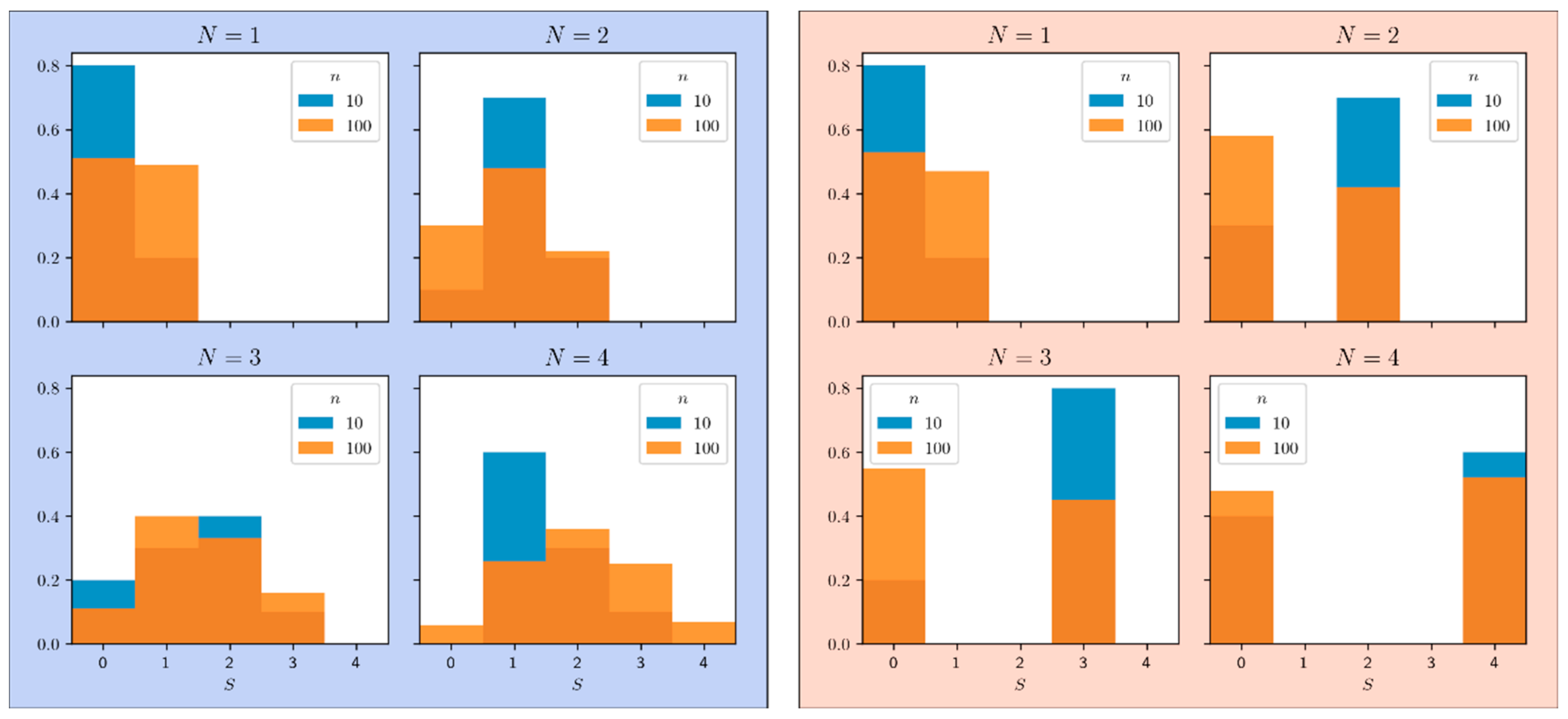
where the dispersion is maximal, i.e., ${\Sigma }^2=1/4$. The histograms are plotted in Figure 1 for a number $n$ of gamblers ranging from $10$ to $100$ and a number $N$ of draws ranging from $1$ to $4$. Equation (3) shows that if $N=1,$ the variance $Va{r}_1\left[S\right]=\Phi \left(1-\Phi \right)$ does not depend on the dispersion of chances ${\Sigma }^2$. As a matter of fact, when $N=1$, the gains are either $0$ or $1$ so that the histogram of gains has only two bins, one at $0$, the other at $1$. The mean of gains is $\Phi$ and the variance is $\Phi \left(1-\Phi \right)$. Neither the mean nor the variance depends on the dispersion of chances ${\Sigma }^2$. Moreover, according to Equation (1), the histogram of gains itself depends only on the mean of the distribution $f\left(p\right)$:

$$\begin{gathered} P_1\left[S=0\right]=E\left[1-p\right]=1-\Phi \\ \begin{array}{c}{P}_1\left[S=1\right]=E\left[p\right]=\Phi \end{array} \end{gathered}$$

(4)

The histogram of gains, therefore, cannot provide information on the dispersion of chances, as shown in Figure 1 for the case $N=1$ where the histograms for $f_0$ and $f_1$ are indistinguishable. This means that a simple draw is not enough to extract the variance of $f\left(p\right)$ from the histogram of gains; multiple draws are necessary, though are they sufficient?

3. A Statistical Test of the Dispersion of Chances

We then note in Figure 1 that the histogram of gains for two draws ($N=2)$ has three bins, one at $0$, the second at $1$ and the third at $2$, with the following values:

$$\begin{gathered} P_2\left[S=0\right]=E\left[{\left(1-p\right)}^2\right]={\left(1-\Phi \right)}^2+{\Sigma }^2 \\ \begin{array}{c}{P}_2\left[S=1\right]=E\left[2p\left(1-p\right)\right]=2\Phi \left(1-\Phi \right)-2{\Sigma }^2\end{array} \end{gathered}$$

(5)

$$\begin{array}{c}{P}_2\left[S=2\right]=E\left[p^2\right]={\Phi }^2+{\Sigma }^2\end{array}$$

(6)

Hence, the histogram of gains now depends on (and only on) both the mean and the variance of $f\left(p\right)$. Note that Equation (5) shows that ${\Sigma }^2\le \Phi \left(1-\Phi \right)$, since $P_2\left[S=1\right]\ge 0$; moreover, $\Phi \left(1-\Phi \right)$ is maximal when $\Phi =1/2$. For three or more draws, we could also have access to higher order moments of $f\left(p\right)$. Nevertheless, the minimum condition for the presence of a probability dispersion is that the variance of $f\left(p\right)$ is non-zero. We therefore propose to design a statistical test that will be able to discriminate between both following hypotheses:

Null hypothesis $H_0$: everybody has the same probability $\Phi$ of gain. This means that $f_0\left(p\right)=\delta \left(p-\Phi \right)$ whose mean is $E\left[p\right]=\Phi$ and dispersion ${\Sigma }^2=0$.

Alternative hypothesis $H_1$: $f$ has the same mean $\Phi$ but there is some dispersion of chances among the population, so that some people are luckier than others; hence, $f$ has a non-zero dispersion ${\Sigma }^2$.

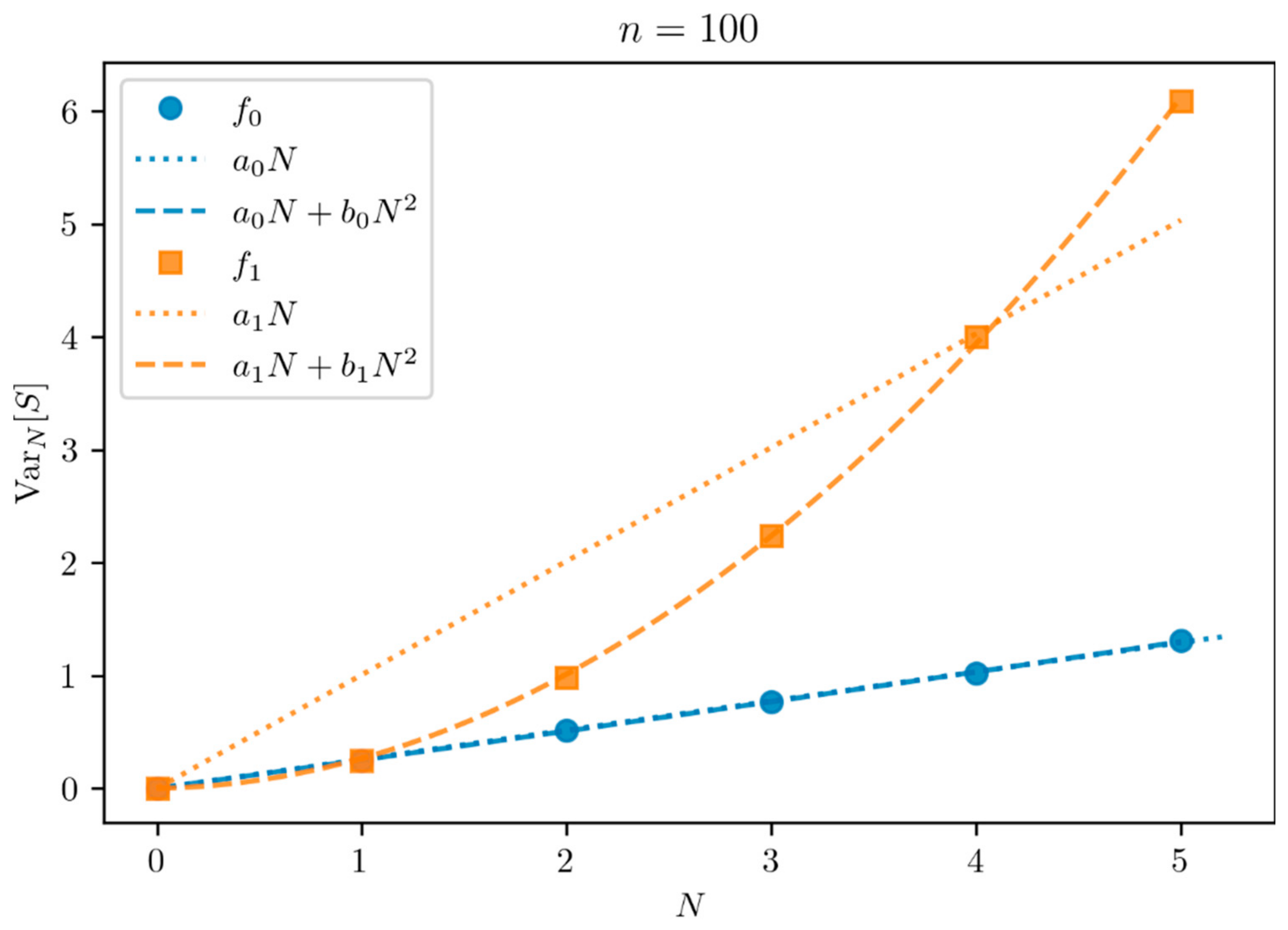
According to $H_0$, the mean of $N$ draws is $\Phi$ and the variance is $N\Phi \left(1-\Phi \right)$, whereas according to $H_1$, the mean of $N$ draws is also $\Phi$ but the variance is $N\left(\Phi \left(1-\Phi \right)-{\Sigma }^2\right)+N^2{\Sigma }^2$. Hence, if the variance $Va{r}_N\left[S\right]$ grows linearly with $N$, then all individuals have the same probability $p$ of success. If, on the contrary, $Va{r}_N\left[S\right]$ grows quadratically with $N$, then not all individuals have the same chance of success. We can, therefore, rephrase our hypothesis test as the following alternative based on the dependence of the variance $Va{r}_N\left[S\right]$ on the number $N$ of draws:

Null hypothesis $H_0$: the variance $Va{r}_N\left[S\right]$ grows linearly with $N$.

Alternative hypothesis $H_1$: the variance $Va{r}_N\left[S\right]$ grows quadratically with $N$.

Figure 2 shows how the variance of $S$ varies as a function of the number of draws $N$ for two typical distributions of mean $1/2$: $f_1$ with zero dispersion and $f_2$ with maximum dispersion $1/4$. The distribution $f_1$ (resp. $f_2$) illustrates the case of a variance growing linearly (resp. quadratically) with $N$.

A relevant statistical test is needed to discriminate between the two hypotheses $H_0$ and $H_1$, or at least to reject the null hypothesis $H_0$. Moreover, in the remainder of this paper, we are particularly interested in the case $N=2$. It is then necessary to reformulate our hypotheses because it becomes difficult to discriminate the quadratic behavior from the linear behavior with only three points. Therefore, we rephrase our hypothesis test, based on the fact that the number of draws is limited to $N=2$:

Null hypothesis $H_0$: the variance of $S$ reads $Va{r}_2\left[S\right]=2\Phi \left(1-\Phi \right)$, i.e., ${\Sigma }^2=0$.

Alternative hypothesis $H_1$: the variance of $S$ reads $Va{r}_2\left[S\right]=2\Phi \left(1-\Phi \right)+2{\Sigma }^2$ with ${\Sigma }^2>0$.

To estimate the variance of $S$ from a sample of $n$ individuals, the unbiased variance estimator is used:

$$V_n=\frac{1}{n-1}{\displaystyle \sum }_{i=1}^n{\left(S_i-\overline{S}\right)}^2$$

where $\overline{S}$ is the mean estimator

$$\overline{S}=\frac{1}{n}{\displaystyle \sum }_{i=1}^n{S}_i$$

The estimation of the variance of $S$, $V_n$, from a sample of finite size $n$ is subject to statistical fluctuations. Thus, our hypotheses become:

Null hypothesis $H_0$: $V_n-2\Phi \left(1-\Phi \right)$ is compatible with 0 considering the error bars, i.e., the standard deviation of $V_n$.

Alternative hypothesis $H_1$: $V_n-2\Phi \left(1-\Phi \right)=2{\Sigma }^2>0$.

The variance of $V_n$ reads (see Appendix A)

$$\begin{array}{c}Va{r}_{{\Sigma }^2}\left[V_n\right]=\frac{2n}{{\left(n-1\right)}^2}\left[\Psi \left(1-2\Psi \right)+7\left(1-4\Psi \right){\Sigma }^2-2{\Sigma }^4\right]+\frac{8}{{\left(n-1\right)}^2}{\left(\Psi +{\Sigma }^2\right)}^2\end{array}$$

(7)

where $\Psi =\Phi \left(1-\Phi \right)$. Its asymptotic expression for $n\gg 1$ reads

$$\begin{array}{c}Va{r}_{{\Sigma }^2}\left[V_n\right]~\frac{2}{n}\left[\Psi \left(1-2\Psi \right)+7\left(1-4\Psi \right){\Sigma }^2-2{\Sigma }^4\right]\end{array}$$

(8)

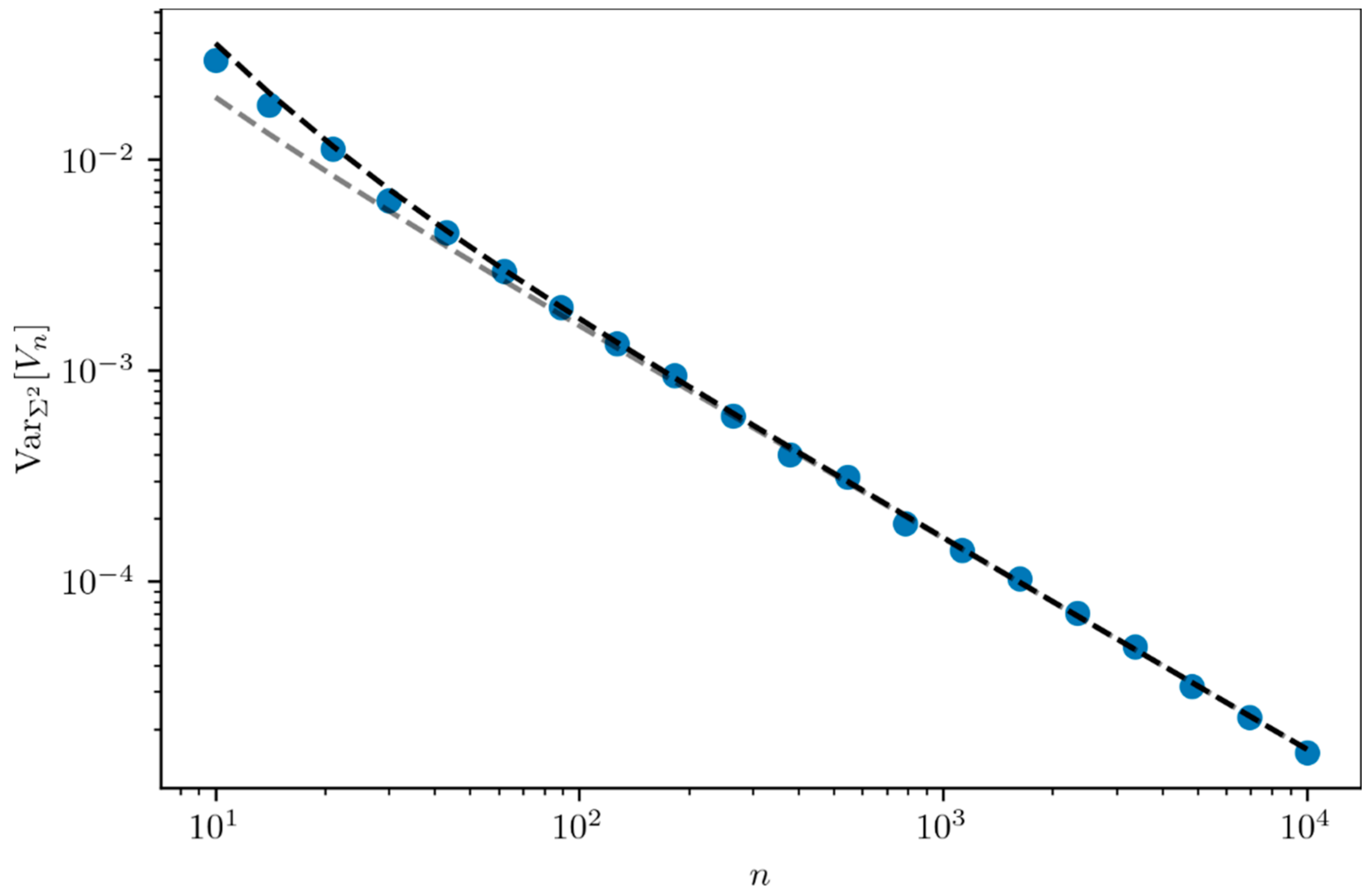
Figure 3 compares the expression of the variance $Va{r}_{{\Sigma }^2}\left[V_n\right]$ (black dashed line) obtained in Equation (7) and its asymptotic expression (grey dashed line) in Equation (8) with simulations (blue dots) and shows good agreement.

It can be noted that the distribution of $V_n$ tends towards a normal distribution $\mathcal{N}\left(E_{{\Sigma }^2}\left[V_n\right],Va{r}_{{\Sigma }^2}\left[V_n\right]\right)$ of mean $E_{{\Sigma }^2}\left[V_n\right]=Va{r}_2\left[S\right]$ and variance $Va{r}_{{\Sigma }^2}\left[V_n\right]$. Now, we wish to estimate the probability of having obtained a value as high as $V_n$ under the null hypothesis $H_0$, i.e., the p-value. Since $V_n$ follows a normal distribution, the p-value can be expressed as follows

$$\begin{array}{c}p\text{-}\mathrm{value}=\frac{1}{2}\left(1-\mathrm{erf}\left(\frac{z}{\sqrt{2}}\right)\right)=\frac{1}{2}\mathrm{erfc}\left(\frac{z}{\sqrt{2}}\right)\end{array}$$

(9)

where $\mathrm{erf}$ and $\mathrm{erfc}$ are, respectively, the error function and the complementary error function. By posing $E_0\left[V_n\right]$ and $Va{r}_0\left[V_n\right]$ as the mean and the variance of $V_n$ under the null hypothesis $H_0$, i.e., ${\Sigma }^2=0$, we have

$$z=\frac{V_n-E_0\left[V_n\right]}{\sqrt{Va{r}_0\left[V_n\right]}}=\frac{V_n-2\Phi \left(1-\Phi \right)}{\sqrt{Va{r}_0\left[V_n\right]}}$$

Within the limit of large sample sizes $n\gg 1$, one can write using, again, $\Psi =\Phi \left(1-\Phi \right)$:

$$z\sim \sqrt{n}\frac{V_n-2\Psi }{\sqrt{2\Psi \left(1-2\Psi \right)}}$$

In the context of Figure 2 restricted to the case $N=2$ and $n=100$, the estimated variance $V_n$ for the distribution $f_1$ (of mean $1/2$ and dispersion $1/4$) leads to $z=20$, i.e., a p-value of ${10}^{-87}$. This allows us to reject the null hypothesis in this case.

4. Dispersion of Disease Risks for Twins

Inequality in disease risk is a major public health issue [8,9]. Of course, part of this inequality is known to depend on genetic and environmental factors. At the turn of the 2000s, a new approach called genome wide association studies (GWAS) was designed to characterize the genetic predisposition to a chronic disease [10]. GWAS are supposed to find in particular the genes involved in a given disease, and among these genes, the variants most at risk, i.e., the DNA sequences of a given gene that are more represented in the people affected by the disease. Such variants characterize the genetic predisposition to the disease. The mean frequency that an individual will become ill in a given population, specified by genetic and environmental factors, can then be measured. As usual, this frequency can be used as a measure of the probability of becoming ill. However, can we assess the dispersion of disease risk, if only it exists, in this specific population? More generally, is there any way to assess the dispersion of risk in a more objective manner, without any a priori assumption on presumed risk factors? Here comes into play a providential help from the existence of twins. Identical twins, also called monozygotic (MZ) twins, have the same genome, shared the same fetal environment and, generally, share the same living conditions. Therefore, they are most likely to also share the same probability of becoming ill, whatever the disease. Identical twins are, therefore, like a player betting twice. This is much related to the gambling question addressed above for $N=2$ (two draws). Indeed, as both twins have the same probability $p$ of having disease $D$, the status—healthy or ill—of each of the two twins is equivalent, respectively, to the outcome—loss or gain—of each of the two draws by one and the same gambler. In this situation, probability $p$ is called a risk. Let $f\left(p\right)$ be the probability distribution function of the risk of having disease $D$ in the population. We define the random variable $S$ as above, i.e., $S=0$ if both twins are healthy, $S=1$ if only one of the two twins is ill and $S=2$ if both twins are ill. The mean $\Phi$ and variance of $S$ are given by Equations (2) and (3), respectively, hence for $N=2$

$$\begin{array}{c}{E}_2\left[S\right]=2\Phi \end{array}$$

(10)

$$Va{r}_2\left[S\right]=2\Phi \left(1-\Phi \right)+2{\Sigma }^2$$

Then, if $V_n$ is significantly greater than $\overline{S}\left(1-\overline{S}/2\right)$, which amounts to carrying out the hypothesis test presented in the above section, we can conclude that there is some dispersion of the disease risk. As we will see below, the dispersion is in fact unusually large. However, before that, let us calculate the twin concordance rate of the disease $D$. In genetics, the twin concordance rate is the probability $\tau$ that a twin is affected given that his/her co-twin is affected:

$$\tau =P\left[X_2=1|X_1=1\right]=\frac{P\left[X_1=1,X_2=1\right]}{P\left[X_1=1\right]}=\frac{P_2\left[S=2\right]}{P\left[X_1=1,X_2=1\right]+P\left[X_1=1,X_2=0\right]}$$

hence

$$\tau =\frac{P_2\left[S=2\right]}{P_2\left[S=2\right]+\frac{1}{2}{P}_2\left[S=1\right]}=\frac{2P_2\left[S=2\right]}{2P_2\left[S=2\right]+P_2\left[S=1\right]}$$

Note that $\tau$ is equal to the probandwise concordance rate, which is known to best assess the twin concordance rate [11].

Using Equations (4) and (6), we can also reformulate the concordance rate of twins in terms of the moments of the distribution $f\left(p\right)$:

$$\begin{array}{c}\tau =\frac{P\left[X_1=1,X_2=1\right]}{P\left[X_1=1\right]}=\frac{P_2\left[S=2\right]}{P_1\left[S=1\right]}=\frac{E\left[p^2\right]}{E\left[p\right]}\end{array}$$

(11)

Note we can generalize the concordance rate for a $N$-tuple:

$${\tau }_N=\frac{P_N\left[S=N\right]}{P_1\left[S=1\right]}=\frac{E\left[p^N\right]}{E\left[p\right]}$$

Using Equations (6) and (10), we obtain

$$\tau =\frac{{\Phi }^2+{\Sigma }^2}{\Phi }$$

Thus, the relative risk $RR=\tau /\Phi$ is equal to

$$\begin{array}{c}RR=\frac{E\left[p^2\right]}{E{\left[p\right]}^2}=\frac{{\Phi }^2+{\Sigma }^2}{{\Phi }^2}=1+\frac{{\Sigma }^2}{{\Phi }^2}\end{array}$$

(12)

The twin concordance rate can also be computed using the probability density function $f_a\left(p\right)$ restricted to the population of affected people. Let $f\left(X, p\right)$ be the joint probability of an individual to have a risk $p\in \left[0,1\right]$ and to be in the state $X\in \left\{0,1\right\}$. According to Bayes’ theorem, also known as the theorem of the probability of causes since it was independently rediscovered by Laplace [12], we write

$$f\left(X, p\right)=f\left(p|X\right)P\left(X\right)=f\left(X|p\right)f\left(p\right)$$

hence

$$f\left(p|X\right)=\frac{f\left(X|p\right)f\left(p\right)}{P\left(X\right)}$$

Then, $f\left(p|X=1\right)$ is the distribution of the risk $p$ in the population of affected people

$$f\left(p|X=1\right)=f_a\left(p\right)$$

Now, by definition, we have

$$f\left(X=1|p\right)=p$$

and by noting that $P\left[X=1\right]=P_1\left[S=1\right]$, we also have

$$P\left[X=1\right]=E\left[f\left(X=1|p\right)\right]=E\left[p\right]$$

This leads to the following expression of the risk distribution function among affected people

$$f_a\left(p\right)=\frac{pf\left(p\right)}{E\left[p\right]}$$

Note that $f_a\left(p\right)$ is the so-called “size-biased law” of the risk $p$ of becoming ill. Size-biased laws are found in many contexts, notably rare events [13], Poisson point processes [14] or familial risk of disease [15].

The mean risk in the affected population is then

$$E_a\left[p\right]={{\displaystyle \int }}_0^{1}p{f}_a\left(p\right)dp=\frac{{{\displaystyle \int }}_0^1{p}^{2}f\left(p\right)dp}{E\left[p\right]}=\frac{E\left[p^2\right]}{E\left[p\right]}$$

where $E_a\left[\cdot \right]$ is the expected value of $\cdot$ among affected people, with the probability distribution $f_a\left(p\right)$. Using Equation (11), we obtain

$$E_a\left[p\right]=\tau$$

which proves that the mean risk in the affected population is equal to the twin concordance rate.

We proceed now to evaluate the functional form of the distribution $f\left(p\right)$. Using the prevalence and the twin concordance rate of the disease $D$, we have access to, and only to, the mean $\Phi$ and dispersion ${\Sigma }^2$ of $f\left(p\right)$. The principle of maximum entropy then provides us with the least arbitrary distribution [16,17]. Dowson and Wragg proved [18] that in the class $P$ of absolutely continuous probability distributions on $\left[0,1\right]$ with given first and second moments (i.e., given mean and variance), there exists a distribution in $P$ which maximizes the entropy

$$H\left[f\right]=-{{\displaystyle \int }}_0^{1}f\left(p\right)\ln f\left(p\right)dp$$

(13)

and the corresponding density function $f\left(p\right)$ on $\left[0,1\right]$ is a truncated normal distribution $f\left(p;m,s,0,1\right)$, which may be either bell-shaped or U-type. Dowson and Wragg show that when $\Phi \ll 1$ and $\Sigma >\Phi$, which is usual for most if not all chronic diseases (unpublished results), the distribution $f\left(p;m,s,0,1\right)$ is U-type (see Appendix B). This distribution, which will be simply denoted $f\left(p;m,s\right)$ in the following, can then be written

$$f\left(p;m,s\right)=\frac{1}{sZ}\sqrt{\frac{2}{\pi }}\exp \left(\frac{{\left(p-m\right)}^2}{2s^2}\right)$$

with

$$Z=\mathrm{erfi}\left(\frac{m}{s\sqrt{2}}\right)+\mathrm{erfi}\left(\frac{1-m}{s\sqrt{2}}\right)$$

The imaginary error function $\mathrm{erfi}\left(x\right)$ can be expressed using the Dawson function $D\left(x\right)$

$$\mathrm{erfi}\left(x\right)=\frac{2}{\sqrt{\pi }}{e}^{x^2}D\left(x\right)$$

Therefore, $f\left(p;m,s\right)$ can finally be written

$$f\left(p;m,s\right)=\frac{1}{\sqrt{2}s}\frac{\exp \left(\frac{p^2-2mp}{2s^2}\right)}{D\left(\frac{m}{s\sqrt{2}}\right)+e^{\frac{1-2m}{2s^2}}D\left(\frac{1-m}{s\sqrt{2}}\right)}$$

It is straightforward to express $\Phi$ and ${\Sigma }^2$ in terms of the parameters $m$ and $s$:

$$\begin{array}{c}\Phi =m-\frac{\sqrt{2}}{2}s\frac{1-e^{\frac{1-2m}{2s^2}}}{D\left(\frac{m}{s\sqrt{2}}\right)+e^{\frac{1-2m}{2s^2}}D\left(\frac{1-m}{s\sqrt{2}}\right)}\end{array}$$

(14)

$$\begin{array}{c}{\Sigma }^2=-s^2\left\{1-\frac{1}{s}\frac{\sqrt{2}}{2}\frac{m+\left(1-m\right)e^{\frac{1-2m}{2s^2}}}{D\left(\frac{m}{s\sqrt{2}}\right)+e^{\frac{1-2m}{2s^2}}D\left(\frac{1-m}{s\sqrt{2}}\right)}+\frac{1}{2}\frac{{\left(1-e^{\frac{1-2m}{2s^2}}\right)}^2}{{\left[D\left(\frac{m}{s\sqrt{2}}\right)+e^{\frac{1-2m}{2s^2}}D\left(\frac{1-m}{s\sqrt{2}}\right)\right]}^2}\right\}\end{array}$$

(15)

Inverting this system of equations to obtain the risk distribution function of the disease $D$ in terms of $\Phi$ and ${\Sigma }^2$ is a bit trickier and requires a numerical solver. In the next section, we show the outcome of this general formalism for one specific chronic disease, namely Crohn’s disease.

5. Application to Crohn’s Disease (CD)

Crohn’s disease (CD) is one of the most well-documented chronic diseases, particularly in the field of genetics [19]. Its prevalence $\Phi$ and twin concordance rate $\tau$ are [20]:

$$\begin{gathered} \Phi \cong 0.0025 \\ \tau \cong 0.385 \end{gathered}$$

Then, the twin relative risk is

$$RR\cong 154$$

hence

$$\begin{gathered} {\Sigma }^2={\Phi }^2\left(RR-1\right)\cong 0.00096 \\ \Sigma \cong 0.031 \end{gathered}$$

which means that

$$\frac{\Sigma }{\Phi }\cong 12$$

(16)

The dispersion of the risk of being affected is, therefore, huge for CD.

It is now necessary to calculate the p-value according to Equation (9) in order to be able to reject (or not) our null hypothesis $H_0$. To do this, we first need to estimate the number of twin pairs $n$ that remains unknown in the Swedish study [20]. Nevertheless, the number of twin pairs with at least one affected twin is known and equal to $n_1+n_2=31.5$, where $n_1=24$ and $n_2=7.5$ are the number of discordant and concordant twin pairs, respectively [20]. We can reconstruct the sample size $n$ that would have been needed to obtain $n_1$ and $n_2$, with probabilities $P_2\left[S=1\right]$ and $P_2\left[S=2\right]$:

$$P_2\left[S=1\right]+P_2\left[S=2\right]=\frac{n_1+n_2}{n}$$

By using Equations (5) and (6), we obtain the following sample size

$$n=\frac{n_1+n_2}{1-{\left(1-\Phi \right)}^2-{\Sigma }^2}\cong 7809$$

Equation (9) is used by calculating $z$ within the limit of large sample sizes $n\gg 1$. This results in $z\approx 2.4$, which allows us to reject the null hypothesis $H_0$ with the $p\text{-}\mathrm{value}\approx 8\cdot {10}^{-3}$.

It is then legitimate to calculate the parameters $m$ and $s$ of the truncated normal distribution $f\left(p;m,s,0,1\right)$, which maximizes the entropy $H\left[f\right]$ given the mean $\Phi$ and the dispersion ${\Sigma }^2$. Solving the system of Equations (14) and (15) for $\Phi =0.0025$ and $\Sigma =0.031$ gives

$$\begin{gathered} m\approx 0.505 \\ s\approx 0.0278 \end{gathered}$$

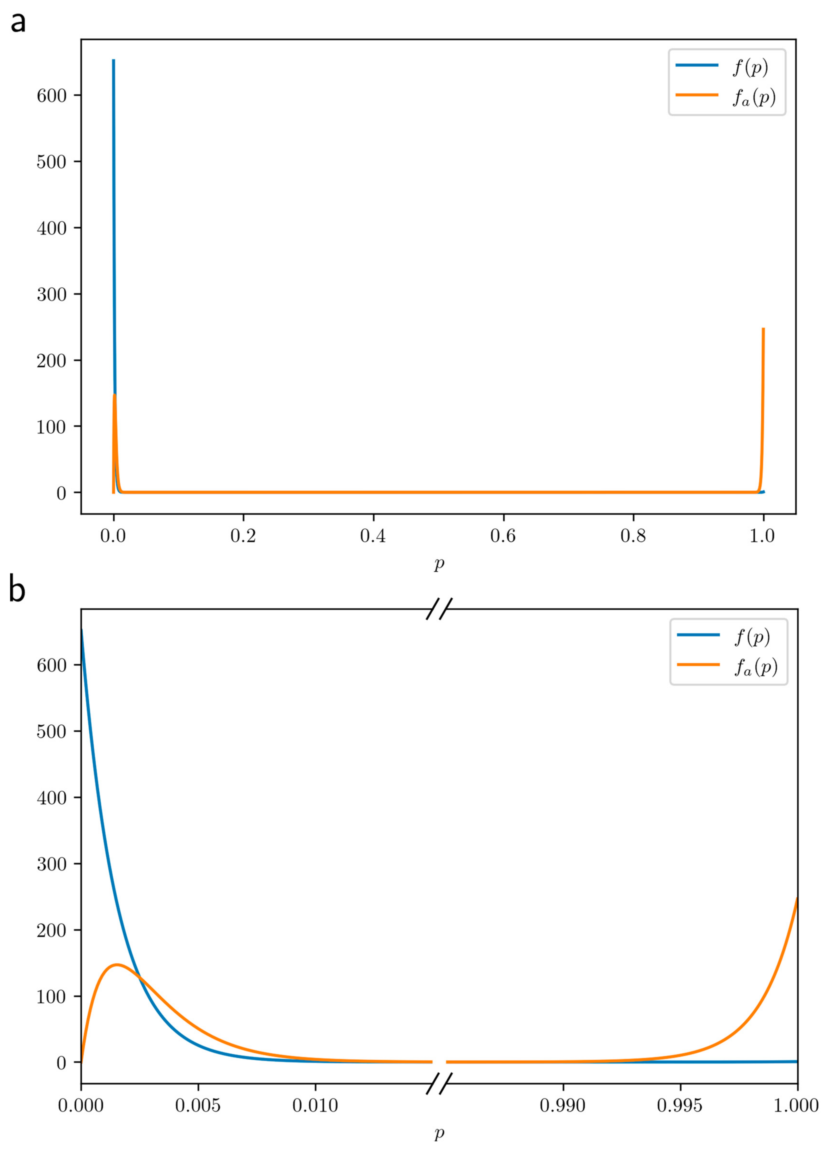
Both probability distribution functions $f\left(p;m,s\right)$ and $f_a\left(p;m,s\right)=pf\left(p;m,s\right)/\Phi$ for CD are plotted in Figure 4a and zoomed in in Figure 4b. Quite remarkably, the probability density function $f_a\left(p;m,s\right)$ in the population of affected people has two narrow peaks, one close to $p=0$ and the other one close to $p=1$. This means that there are two quite separate categories of people who become ill: in the left peak (close to $p=0$), people are at very low risk, but still have been unlucky to become ill, whereas in the right peak (close to $p=1$), people are at extremely high risk, hence are unlucky a priori, and indeed, were bound to become ill. Not having any luck (to become ill because of high risk) or to have been unlucky (to become ill despite low risk), that is the question!

Finally, we note that concordant twins are very likely to be in the right peak, whereas discordant twins are in the left one. Indeed, when two MZ twins have their common risk $p$ in the left peak, their probability of being concordant is extremely low, of the order of the mean of $p^2$ restricted to the left peak of $f_a\left(p\right)$, which is of the order of ${10}^{-5}$. On the contrary, when two MZ twins have their common risk $p$ in the right peak, their probability to be concordant is extremely high, of the order of $0.997$. Interestingly enough, the fraction of people in the right peak (area under the curve) is $38.52\%$, quite similar to the (probandwise) twin concordance rate of $38.65\%$ [20]. This strongly suggests that concordant twins for a given disease both have a strong predisposition for this disease, whereas discordant twins both have no particular predisposition.

6. Conclusions

Assessing the inequality of chances in a given population is a critical problem that has several issues, notably health and social opportunity. Starting with the simple heads or tails game, we have shown that, although hidden variables such as ex ante chances of gamblers (possibly cheating) cannot be assessed, their distribution can actually be assessed whenever multiple draws are available. For this purpose, we have proposed a hypothesis test to evidence the inequality of chances in a given population, then infer the functional form of the probability distribution function of the ex ante chances by means of the principle of maximum entropy, which gives the least arbitrary distribution given the mean and variance of the probability distribution function.

We applied this methodology to chronic diseases and found that the distribution of the risk of becoming ill is usually a U-type truncated normal distribution. We have computed the parameters of this U-type distribution in the case of Crohn’s disease using the prevalence and the twin concordance rate of this pathology. Moreover, we have found that the risk distribution function among affected people is bimodal with two narrow peaks, one corresponding to people with no liable risk factor and the other one to people genetically or environmentally destined to become ill. An interesting consequence is that concordant twins for a given disease both have a strong predisposition for that disease, while discordant twins both have no particular predisposition.

One should still not over-interpret the results, as they still rely only on estimates of the prevalence and the twin concordance rate of the disease. It can be thought of as the best possible interpretation in terms of distribution, based on the available information. Nevertheless, maximizing the entropy of the risk distribution function leads to significantly different conclusions than more arbitrary distributions such as, for example, beta-distributions [21].

Twins provide a unique means to play twice at the lottery of diseases. Of course, twins are all the more relevant to assess ex ante chances as they share the same environmental factors. In the same vein, “social twins” or more generally “social clones” would be of great help in assessing inequality of opportunities. However, controlling the environment of such social clones would be rather challenging as the issue of choice comes into play, which may change people’s lives with the same opportunities. Assessing the inequality of opportunities is, therefore, one of the most delicate, almost completely open, issues.

Pascal could never complete his treatise “Geometry of Chance”. This never-ending treatise is still being written, as evidenced in this Special Issue.

References

- Debnath, L.; Basu, K. A short history of probability theory and its applications. Int. J. Math. Educ. Sci. Technol. 2014, 46, 13–39. [Google Scholar] [CrossRef]
- Godfroy-Génin, A.-S. Pascal: The geometry of chance. Math. Sci. Hum. 2000, 150, 7–39. [Google Scholar]
- Maxwell, J.C. Illustrations of the Dynamical Theory of Gases. Part I. On the motions and collisions of perfectly elastic spheres. Lond. Edinb. Dublin Philos. Mag. J. Sci. 1860, 19, 19–32. [Google Scholar] [CrossRef]
- Stern, O. Eine direkte Messung der thermischen Molekulargeschwindigkeit. Z. Phys. 1920, 2, 49. [Google Scholar] [CrossRef] [Green Version]
- Gerlach, W.; Stern, O. Moment Das magnetische des Silberatoms. Z. Phys. 1922, 9, 353–355. [Google Scholar] [CrossRef]
- Bruza, P.D.; Wang, Z.; Busemeyer, J.R. Quantum cognition: A new theoretical approach to psychology. Trends Cogn. Sci. 2015, 19, 383–393. [Google Scholar] [CrossRef] [Green Version]
- Corbett, S.; Courtiol, A.; Lummaa, V.; Moorad, J.; Stearns, S. The transition to modernity and chronic disease: Mismatch and natural selection. Nat. Rev. Genet. 2018, 19, 419–430. [Google Scholar] [CrossRef]
- Arcaya, M.C.; Arcaya, A.L.; Subramanian, S.V. Inequalities in health: Definitions, concepts, and theories. Glob. Health Action 2015, 8, 27106. [Google Scholar] [CrossRef]
- Gomes, M.G.M.; Oliveira, J.F.; Bertolde, A.; Ayabina, D.; Nguyen, T.A.; Maciel, E.L.; Duarte, R.; Nguyen, B.H.; Shete, P.B.; Lienhardt, C. Introducing risk inequality metrics in tuberculosis policy development. Nat. Commun. 2019, 10, 2480. [Google Scholar] [CrossRef] [Green Version]
- Tam, V.; Patel, N.; Turcotte, M.; Bossé, Y.; Paré, G.; Meyre, D. Benefits and limitations of genome-wide association studies. Nat. Rev. Genet. 2019, 20, 467–484. [Google Scholar] [CrossRef]
- McGue, M. When assessing twin concordance, use the probandwise not the pairwise rate. Schizophr. Bull. 1992, 18, 171–176. [Google Scholar] [CrossRef]
- Stigler, S.M. Memoir on the Probability of the Causes of Events, Pierre Simon Laplace. Statist. Sci. 1986, 1, 364–378. [Google Scholar] [CrossRef]
- Patil, G.P.; Rao, C.R. Weighted distributions and size-based sampling with applications to wildlife populations and human families. Biometrics 1978, 34, 179–189. [Google Scholar] [CrossRef] [Green Version]
- Mihael, P.; Jim, P.; Marc, Y. Size-biased sampling of Poisson point processes and excursions. Probab. Theory Relat. Fields 1992, 92, 21–39. [Google Scholar]
- Davidov, O.; Zelen, M. Referent sampling, family history and relative risk: The role of length-biased sampling. Biostatistics 2001, 2, 173–181. [Google Scholar] [CrossRef]
- Pressé, S.; Ghosh, K.; Lee, J.; Dill, K.A. Principles of maximum entropy and maximum caliber in statistical physics. Rev. Mod. Phys. 2013, 85, 1115–1141. [Google Scholar] [CrossRef] [Green Version]
- Cofré, R.; Herzog, R.; Corcoran, D.; Rosas, F.E. A Comparison of the Maximum Entropy Principle Across Biological Spatial Scales. Entropy 2019, 21, 1009. [Google Scholar] [CrossRef] [Green Version]
- Dowson, D.C.; Wragg, A. Maximum-Entropy Distributions Having Prescribed First and Second Moments. IEEE Trans. Inf. Theory 1973, 19, 689–693. [Google Scholar] [CrossRef]
- Verstockt, B.; Smith, K.G.C.; Lee, J.C. Genome-wide association studies in Crohn’s disease: Past, present and future. Clin. Transl. Immunol. 2018, 7, e1001. [Google Scholar] [CrossRef]
- Halfvarson, J. Genetics in twins with Crohnʼs disease: Less pronounced than previously believed? Inflamm. Bowel Dis. 2011, 17, 6–12. [Google Scholar] [CrossRef]
- Stensrud, M.J.; Valberg, M. Inequality in genetic cancer risk suggests bad genes rather than bad luck. Nat. Commun. 2017, 8, 1165. [Google Scholar] [CrossRef] [PubMed] [Green Version]
Figure 1.
Simulated histograms of gains for two distributions and : on the left-hand side and on the right-hand side . In each case, the histogram of success is plotted for increasing values of the number of draws () and for two numbers of gamblers: (in blue) and (in orange). For , note that the histogram for is similar to the histogram for and both histograms converge to the same limit as goes to infinity. On the contrary, for each , the histograms for and diverge as increases.
Figure 2.
Linear regression fits for (blue dotted line), with in agreement with Equation (3) when . Moreover, agrees with the expected value . The quadratic fit (blue dashed line) yields an equivalent result. At odds with , the linear regression does not fit for (orange dotted line), whereas the quadratic fit (orange dashed line) is excellent, with: and . Here, agrees with the expected value and with the expected value .
Figure 3.
Evolution of the variance of for as a function of the number of players. The blue dots are simulated with and . The black dashed line corresponds to the variance of according to Equation (7). The grey dashed line corresponds to the leading-order term in of the expected variance in Equation (8).
Figure 4.
(a) CD risk distribution function among the population (in blue) is narrow peaked at . The risk distribution function among affected people (in orange) has two narrow peaks. (b) Zoom in the vicinity of both peaks and . Concordant twins (almost) all belong to the right peak (at ) whereas discordant twins (almost) all belong to the left peak (at ).
Publisher’s Note: MDPI stays neutral with regard to jurisdictional claims in published maps and institutional affiliations. |
© 2021 by the authors. Licensee MDPI, Basel, Switzerland. This article is an open access article distributed under the terms and conditions of the Creative Commons Attribution (CC BY) license (https://creativecommons.org/licenses/by/4.0/).
Share and Cite
MDPI and ACS Style
Lesage, A.; Victor, J.-M. To Be or to Have Been Lucky, That Is the Question. Philosophies 2021, 6, 57. https://0-doi-org.brum.beds.ac.uk/10.3390/philosophies6030057
AMA Style
Lesage A, Victor J-M. To Be or to Have Been Lucky, That Is the Question. Philosophies. 2021; 6(3):57. https://0-doi-org.brum.beds.ac.uk/10.3390/philosophies6030057
Chicago/Turabian StyleLesage, Antony, and Jean-Marc Victor. 2021. "To Be or to Have Been Lucky, That Is the Question" Philosophies 6, no. 3: 57. https://0-doi-org.brum.beds.ac.uk/10.3390/philosophies6030057