Improved Sum of Residues Modular Multiplication Algorithm


Department of Computing, Macquarie University, Sydney 2109, Australia
Cryptography 2019, 3(2), 14; https://0-doi-org.brum.beds.ac.uk/10.3390/cryptography3020014
Submission received: 26 April 2019
/
Revised: 27 May 2019
/
Accepted: 27 May 2019
/
Published: 29 May 2019
Abstract
:Modular reduction of large values is a core operation in most common public-key cryptosystems that involves intensive computations in finite fields. Within such schemes, efficiency is a critical issue for the effectiveness of practical implementation of modular reduction. Recently, Residue Number Systems have drawn attention in cryptography application as they provide a good means for extreme long integer arithmetic and their carry-free operations make parallel implementation feasible. In this paper, we present an algorithm to calculate the precise value of “” directly in the RNS representation of an integer. The pipe-lined, non-pipe-lined, and parallel hardware architectures are proposed and implemented on XILINX FPGAs.
1. Introduction
The residue number system (RNS) has been proposed by Svoboda and Valach in 1955 [1] and independently by Garner in 1959 [2]. It uses a base of co-prime moduli to split an integer X into small integers where is the residue of X divided by denoted as or simply .
Conversion to RNS is straightforward. Reverse conversion is complex and uses the Chinese Remainder Theorem (CRT) [3]. Addition, subtraction, and multiplication in RNS are very efficient. These operations are performed on residues in parallel and independently, without carry propagation between them. The natural parallelism and carry-free properties speed up computations in RNS and provide a high level of design modularity and scalability.
One of the most interesting developments has been the applications of RNS in cryptography [3]. Some cryptographic algorithms which need big word lengths ranging from 2048 bits to 4096 bits like RSA (Rivest-Shamir-Adleman) algorithm [4], have been implemented in RNS [5,6]. RNS is also an appealing method in Elliptic Curve Cryptography (ECC) where the sizes range from 160 to 256 bits.
The modular reduction is the core function in public key cryptosystems, where all calculations are done in a finite field with characteristic p.
The first RNS modular reduction proposed by Karl and Reinhard Posch [7] in 1995 was based on the Montgomery reduction algorithm [8]. Their proposed algorithm needed two RNS base extension operations. They used a floating point computation for correction of the base extension in their architecture that was not compatible with the RNS representation.
The main advantage of the RNS Montgomery reduction method is its efficiency in using hardware resources. In this algorithm, half of the RNS channels are involved at a time. Two base extension operations are used to retrieve the other half of the RNS set. The base extension is a costly operation and limits the speed of the algorithm. In 1998, Bajard et al. [9] introduced a new Montgomery RNS reduction architecture using mixed radix system (MRS) [3] representation for base extensions. Due to the recursive nature of MRS, this method is hard to implement in the hardware. Based on Shenoy and Kumaresan work in [10], Bajard et al. proposed a Montgomery RNS modular reduction algorithm in 1998, using residue recovery for the base extension [11]. In 2000, the floating point approach of [7] was improved by Kawamura et al. [12] by introducing the cox-rower architecture that is well adapted to hardware implementation. In 2014, Bajard and Merkiche [13] proposed an improvement in cox-rower architecture by introducing a second level of Montgomery reduction within each RNS unit. Several variants and improvements on the RNS montgomery modular reduction have been discussed in the literature [2,14,15,16,17]. The most recent work in [18] proposed the application of quadratic residues in the RNS Montgomery reduction algorithm.
Modular reduction based on the sum of residues (SOR) algorithm was first presented by Phillips et al. [19] in 2010. The SOR algorithm hardware implementation was proposed later in [20]. A disadvantage of the SOR algorithm is that unlike the Montgomery reduction method, the output is an unknown and variable factor of the “” value. Although this algorithm offers a high level of parallelism in calculations, the proposed implementation in [20] is considerably big in area.
In this paper, we do an improvement to the sum of residues algorithm by introducing the correction factor to obtain a precise result. Using an efficient moduli set, we also propose a new design to improve the area in comparison to [20]. The timing of our design is improved compared to RNS Montgomery reduction as well. Two implementations are done for the 256-bit prime field of the SEC2P256K1 [21] and the 255-bit prime field of the ED25519 [22] elliptic curves respectively. It can be extended to other prime fields using the same methodology.
Section 2 of this paper is a quick review of the sum of residues reduction algorithm and the related works already published in the literature. Section 3 is mainly our contribution to the correction of the sum of residues algorithm and improving speed and area using efficient RNS base (moduli set). Section 4 presents our proposed hardware architectures and implementation results. Table A1 in Appendix A summarises the notations applied in this paper.
2. Background
Representation of the integer X, , using CRT (Chinese Reminder Theorem) is [3]:
where, N is the number of moduli in moduli set of co-primes .
.
(also called dynamic range of X).
and
is the multiplicative inverse of . In other terms, .
We assume that: . As a result, the dynamic range is .
The values of M, , and are known and pre-computed for hardware implementation.
Consider two l-bit integer X and Y. The multiplication result is a -bit integer. The representation of Z in RNS is:
where, .
The CRT enforces condition . Otherwise, the N-tuple RNS set in (2) do not represent the correct integer Z. In other terms, the bit length of the moduli (n) and the number of moduli (N) must be chosen such that the condition is satisfied.
Introducing , the integer Z can be presented as:
An integer coefficient can be found such that [3]:
Reducing Z by the modulus p yields:
The RNS multiplications and can be easily performed by an unsigned integer multiplier and a modular reduction detailed in Section 2.1. Calculation of is outlined in Section 2.2.
2.1. Efficient RNS Modular Reduction
An RNS modular multiplication in the 256-bit prime field requires a dynamic range of at least 512 bits. In our design this is provided by eight 66-bit pseudo-Mersenne co-prime moduli as presented in Table 1. This moduli set provides a 528-bit dynamic range.
The optimal RNS bases are discussed in [23]. Modular reduction implementation using moduli set in general form of (here ) is very fast and low-cost in hardware [24]. Suppose B is a -bit integer (). It can be broken up into two n-bit most significant and least significant integers denoted as and respectively. In other terms, .
Since , then:
has bits and can be re-written as .
Let , be the binary representation of . Then we introduce as the most significant bits of , i.e. and as the rest least significant bits left shifted times, i.e. .
Similarly,
Since is bits long, the term can be rewritten as concatenation of to itself, i.e., . (“” denotes bit concatenation operation.)
So, the final result is:
The modular reduction of can be calculated at the cost of one 4-input n-bit CSA (Carry Save Adder) compare to Barrett method [25] that requires two multipliers.
2.2. Calculation of
Since , then:
It is known that: , therefore:
Calculation of has been discussed in [12,20]. It is shown that choosing proper constants q and and enforcing boundary condition of (12), can be calculated using (13).
Algorithm 1 is used to calculate the coefficient . A Maple program was written to find the optimal q and . Choosing , for the 66-bit moduli set in Table 1, we realised that is suitable for the whole effective dynamic range. The hardware realisation of (13) is an N-input q-bit adder with offset . Note that the effective dynamic range by applying boundary condition in (12), is ; that is greater than the minimum required bit length (512 bits).
| Algorithm 1: Calculation of |
| input: where, , . input: q, . output: . ;  ; |
3. Improved Sum of Residues (SOR) Algorithm
Here, we introduce an integer V as:
Comparing (5) and (14), it can be realised that the difference is a factor of modulus p. Recalling the fact that for any integer Z we can find an integer such that .
( and are constants such that: , and ).
The factor () is a function of , not a constant. Therefore the value of V—which is actually the output of SOR algorithm introduced in [19,20]—is not presenting the true reduction of . In fact:
The values of and for are known and can be implemented in hardware as pre-computed constants.
The RNS form of V resulted from (14) is:
If (17) deducted by , the accurate value of in RNS will be obtained.
3.1. Calculation of
The coefficient is an integer. Reminding that and , can be calculated as:
The modulus p is considered to be a pseudo Mersenne prime in general form of where . For example: and are the field modulus for the NIST recommended curve SECP256K1 [21] and the Twisted Edwards Curve ED25519 [22], respectively.
Substitution of fractional equation in (20) results:
Considering that and , if we choose:
Then, , and the value of resulted from (21) is:
The condition in (22) provides a new boundary for choosing the field modulus p. It is a valid condition for most known prime modulus p used practically in cryptography. Table 2 shows the validity of for some standard curves based on (23).
The hardware implementation of (23) needs a -bit multiplier. For an efficient hardware implementation, it is essential to avoid such a big multiplier. To compute the value of in hardware, we used:
The integer T must be selected such that the equality of (23) and (24) is guaranteed. Using a MAPLE program, we realised that for SECP256K1 and for ED25519 are the best solutions for an area efficient hardware. In this case, as the term is 55 bits for SECP256K1 and 44 bits for ED25519, the -bit and -bit multipliers are required to compute , respectively.
Therefore, the coefficient of for SECP256K1 can be calculated efficiently by the following equation:
Similarly, for ED25519, can be calculated using the below formula:
The value of can be pre-computed and saved in the hardware for to N. The integer is maximum 52-bit long for SECP256K1 and 42-bit long for ED25519. As a result, RNS conversion is not required. () and can be directly used in RNS calculations.
Calculation of can be done in parallel and will not impose extra delay in the design. Finally, to find we need to compute . Note that is a constant and can be pre-computed as well. So, we get:
The number of operations can be reduced by pre-computing instead of .
(A modular subtraction consists of two operations: , ). Then is calculated directly by:
Algorithm 2 presents the RNS modulo p multiplication over moduli base using improved sum of residues method. The calculations at stages 4 and 5 are done in parallel. Different levels of parallelism can be achieved in hardware by adding on or more RNS multipliers to perform stage 5.3 calculations in a shorter time.
As discussed, the coefficient is a 52-bit(42-bit) integer for SECP256K1(ED25519) design. Consequently, the output of the original SOR algorithm [19] represented in (16) is as big as 308(297) bits. In conclusion, the hardware introduced in [20,26,27] cannot calculate two tandem modular multiplications while the product of the second stage inputs has a higher bit number than the dynamic range that violates the CRT. In cryptographic applications, it is generally required to do multiple modular multiplications. Our correction to the SOR algorithm ensures that the inputs of the next multiplication stage are in range.
| Algorithm 2: Improved Sum of residues reduction |
| Require: p, , q, , , , , T, Require: , , for i = 1 to N Require: pre-computed tables , , and Require: pre-computed table for to N. Require: pre-computed table for to input: Integers X and Y, in form of RNS: and . output: Presentation of in RNS: .  |
4. New SOR Algorithm Implementation and Performance
The required memory to implement pre-computed parameters of Algorithm 2 is bits, where is the biggest bit number of . In our case for SECP256K1 and for ED25519. Therefore, the required memory is 9944 and 9856 bits for the SECP256K1 and ED25519 respectively.
In our design, FPGA DSP modules are used for the realisation of eight bit multipliers that are followed by a combinational reduction logic to build an RNS multiplier. The total number of 128 DSP resources are used for an RNS multiplier. Table 3 lists maximum logic and net delays of the RNS multiplier and the RNS adder(accumulator) implemented on the different FPGA platforms used in this survey. These delays determine the overall design latency and performance. The maximum RNS adder logic and routing latency are less than half of the RNS multiplier logic and net delays. The system clock cycle is chosen such that an RNS addition is complete in one clock period and an RNS multiplication result is ready in two clock periods.
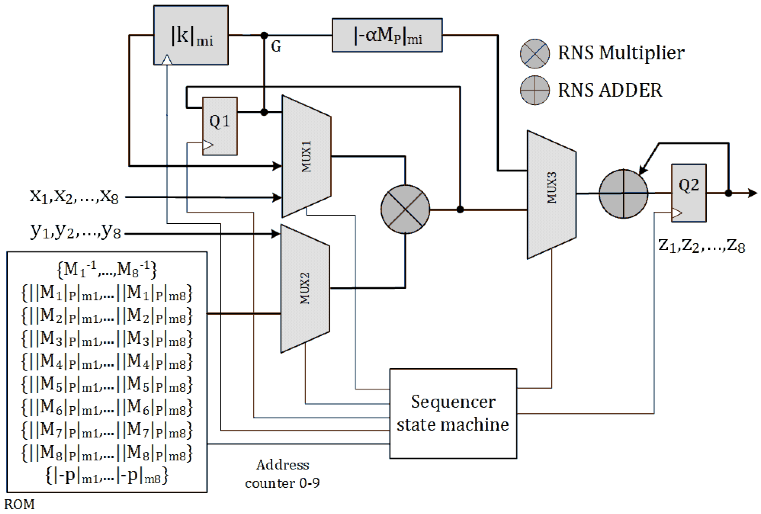
Figure 1 presents a simplified block diagram of the Algorithm 2 with non-pipe-lined architecture. We name this architecture as SOR_1M_N. The sequencer state machine provides select signals of the multiplexers and clocks for internal registers. The inputs of the circuit are two 256-bit integers X and Y in RNS representation over base ; i.e., and respectively.
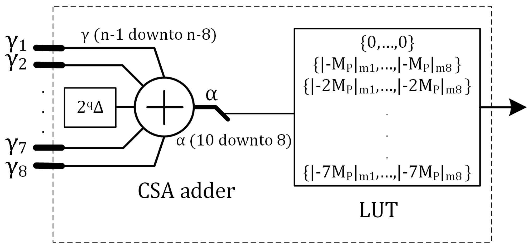
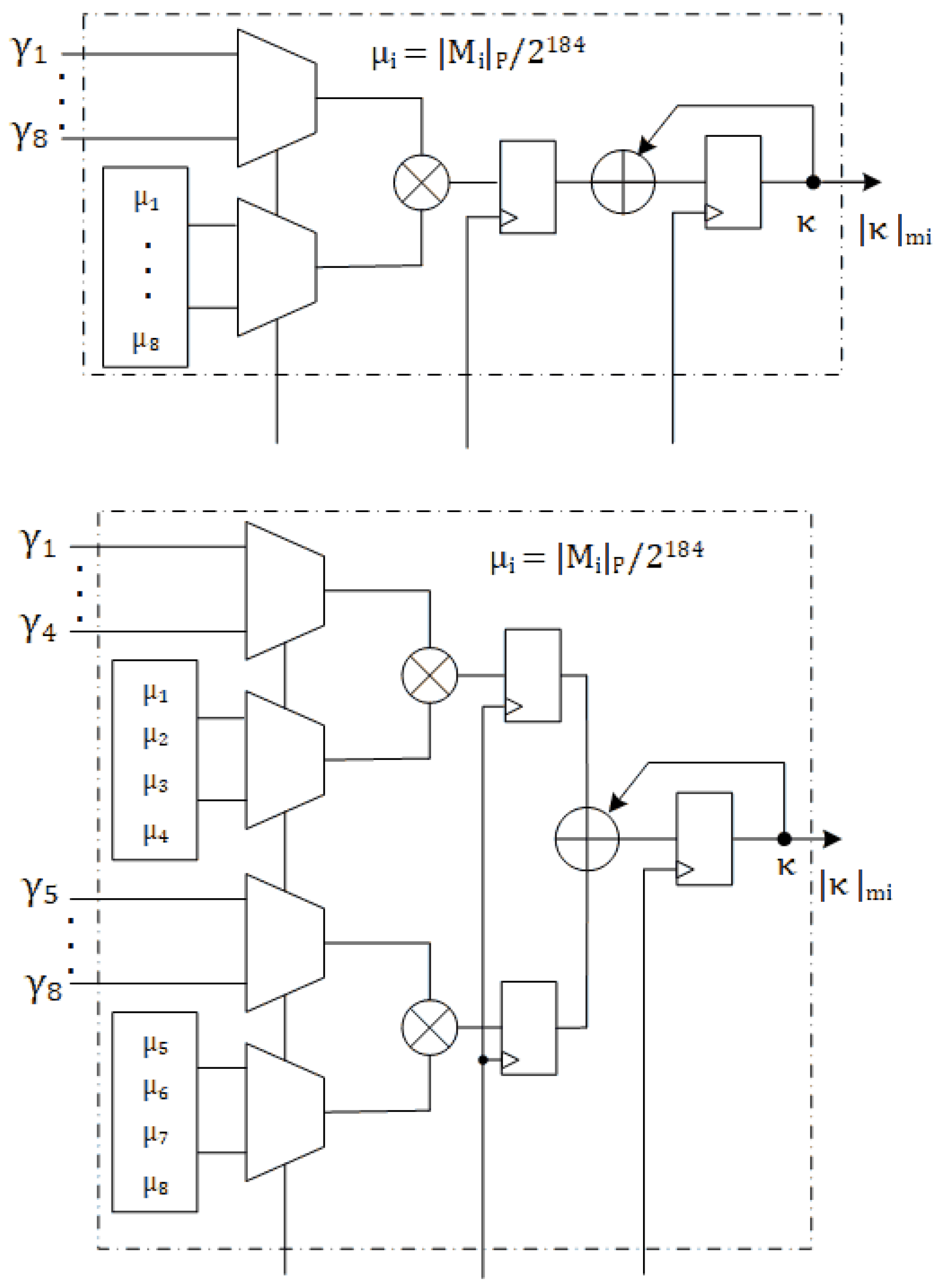
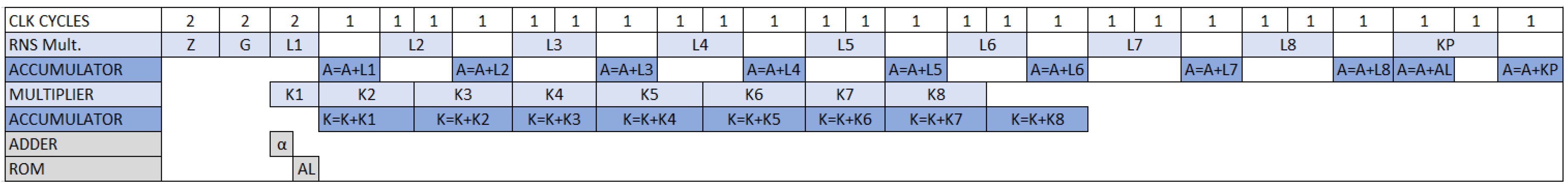
The RNS multiplier inputs are selected by multiplexers MUX1 and MUX2. At the second clock cycle the output of multiplier i.e., is latched by register . At the fourth clock cycle, is calculated and latched by register . The calculation of starts after the fourth clock cycle, by adding the eight most significant bits of to to the offset . The 3 most significant bits of the result are used to select the value of from the Look up table. Figure 2 illustrates the hardware implementation of . At the next clock cycles will be calculated and accumulated in register . The RNS multiplier must be idle for one clock cycle, letting the RNS adder of the accumulator be completed and latched whenever accumulation of the results is required. The value of is calculated in parallel using the hardware shown in Figure 3. The is calculated at the and cycles and will be added to the accumulator Q2 at the last clock cycle. The sum of moduli reduction is completed in clock cycles. Figure A1 in Appendix A shows the data flow diagram of SOR_1M_N architecture at every clock cycle.
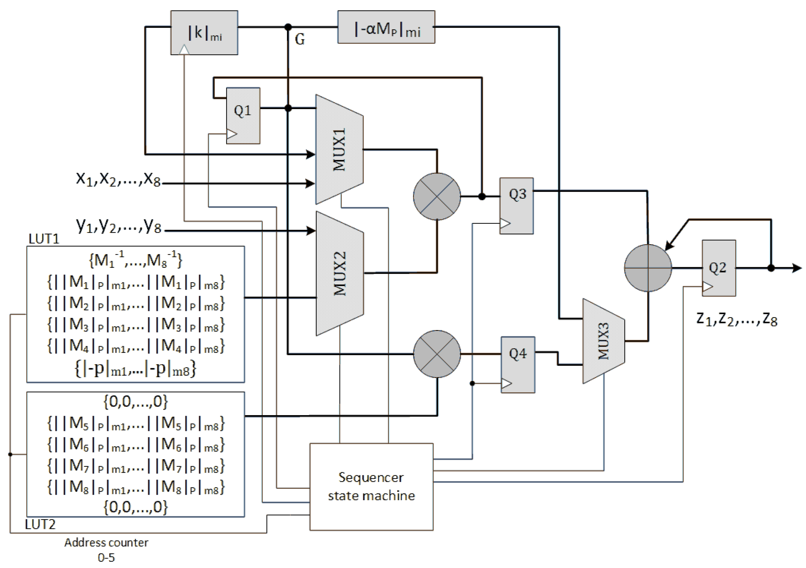
A pipe-lined design is depicted in Figure 4. Here, an extra register Q3 latches the RNS multiplier’s output. So, The idle cycles in SOR_1M_N are removed. We call this design SOR_1M_P. The data flow diagram of SOR_1M_P architecture is illustrated in Figure A2 in Appendix A. Algorithm 2 can be performed in clock cycles using this architecture.
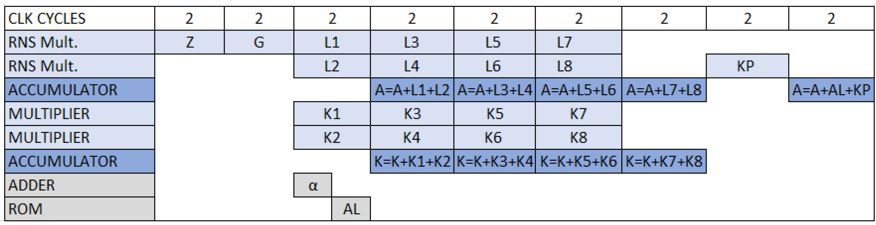
Parallel designs are possible by adding RNS multipliers to the design. Figure 5 shows the architecture of using two identical RNS multipliers in parallel to implement algorithm 2. We tag this architecture as SOR_2M. The calculation of , () is split between two RNS multipliers. So, the required time to calculate all the N terms is halved. As shown in Figure 3, An extra multiplier is also required to calculate in time. The latency of SOM_2M architecture is clock cycles. Theoretically, the latency could be as small as 12 clock cycles using N parallel RNS multipliers. Figure A3 in Appendix A shows the data flow diagram of SOM_2M architecture.
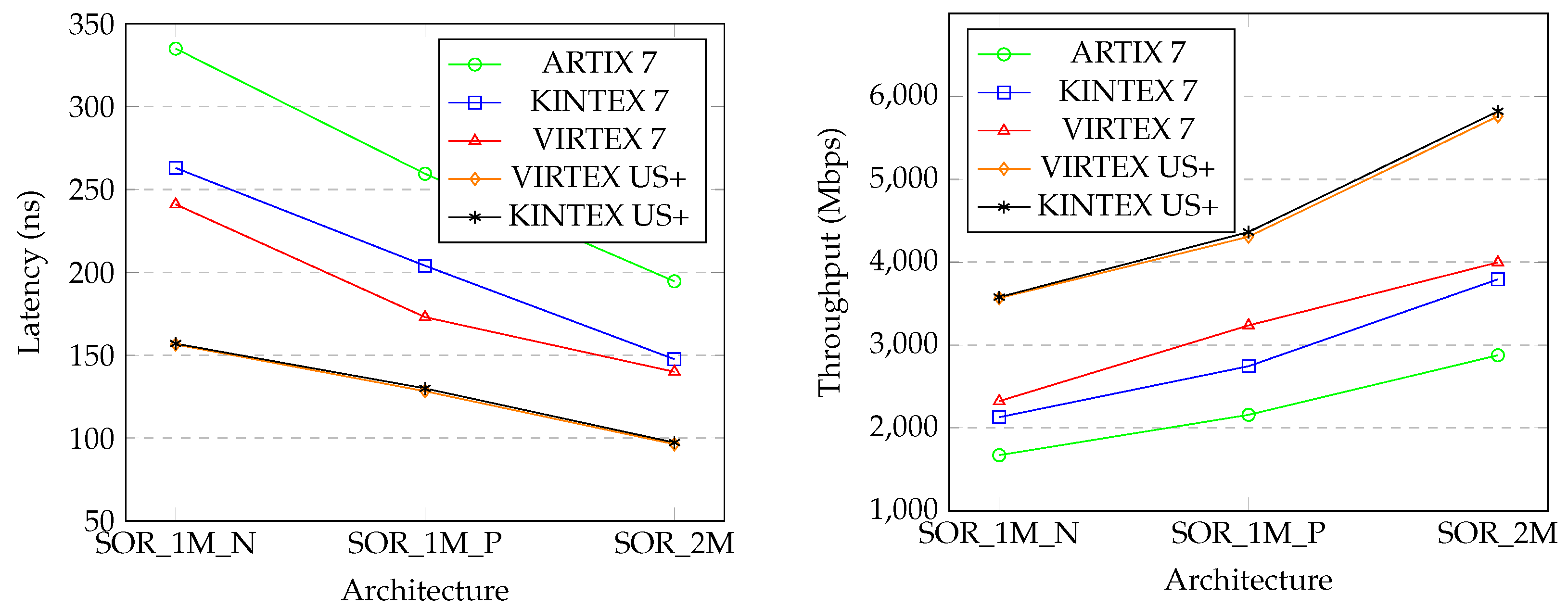
Table 4, shows implementation results on ARTIX 7, VIRTEX 7, KINTEX 7, VIRTEX UltraScale+™, and KINTEX UltraScale+ FPGA series. VIVADO 2017.4 is used for VHDL codes synthesis. On a Xilinx VIRTEX 7 platform, as shown in Table 3, a 66-bit modular multiplication was achieved in 11.525 ns and a 66-bit RNS addition was performed in 3.93 ns. Considering the maximum net delays, clock frequency 125 MHz is achievable. The fastest design is realised using KINTEX UltraScale+ that clock frequency 187.13 MHz is reachable. Figure 6 summarises the latency and throughput of SOR_1M_N, SOR_1M_P, and SOR_2M on different Xilinx FPGA series for ease of comparison.
4.1. Comparison
In Table 5, we have outlined implementation results of recent similar works in the context of RNS. The design in [20] and [27] are based on the SOR algorithm in [19]. Both of them use forty 14-bit co-prime moduli as RNS base to provide a 560-bit dynamic range. Barrett reduction method [25] is used for moduli multiplication at each channel. The Barrett reduction algorithm costs 2 multiplications and one subtraction which is not an optimised method for high-speed designs. The design in [20] is a combinational logic and performs an RNS modular reduction in one clock cycles. The area of this design is reported in [27] which is equivalent to (34.34 KLUTs, 2016 DSPs) for non pipe-lined and (36.5 KLUTs, 2016 DSPs) for pipe-lined architectures. The MM_SPA design in [27], is a more reasonable design in terms of the logic size (11.43 KLUT, 512 DSPs). However, in contrast to our SOR_2M design on VIRTEX-7, it consumes more hardware resources and in terms of speed, it is considerably slower. These designs, are based on SOR algorithm in [19] that is not performing a complete reduction. As discussed in Section 3.1, their outputs can exceed the RNS dynamic range and give out completely incorrect results.
A survey on RNS Montgomery reduction algorithm and the improvements in this context is presented in [18]. The application of quadratic residues in RNS modular reduction is then presented and two algorithms sQ-RNS and dQ-RNS are proposed. The authors used eight 65-bit moduli base for their RNS hardware which is similar to our design. The achieved clock frequencies for these two designs are 139.5 MHz and 142.7 MHz, respectively. The input considered for the algorithms is the RNS presentation of “”; where “x” is equivalent to Z in our notations in Equation (2) and “” is a constant. To do a fair comparison, it is required to consider two initial RNS multiplications to get the input ready for the algorithms sQ-RNS and dQ-RNS. This adds two stages of full range RNS multiplication to the design.
As illustrated on Figure 13 of [18] it takes 3 clock cycles to perform one multiplication and reduction. So, at the maximum working clock frequency, 42 ns will be added to the latency of the proposed RNS modular reduction circuit. As a result, the equivalent latency for an RNS reduction for sQ-RNs and dQ-RNS reduction hardware is 150.53 ns and 168.18 ns, respectively. Consider that the output of these algorithms is a factor of “”, not the precise value of “”. The RNS Montgomery reduction algorithms use half of moduli set. This makes the hardware area efficient, but it still full moduli range multiplication are required for computations. On the same FPGA platform used in [18], i.e., KINTEX Ultra Scale+ ™, we achieved the latency of 128.3 ns and 96.3 ns with our SOR_1M_P and SOR_2M designs, respectively. The latency of SOR_2M showed 36% improvement compare to sQ-RNS and 41.1% improvement in contrast to MM_SPA on similar FPGA platforms. Similarly, there is 14.9% and 27.6% improvement of SOR_1M_P latency in compare to sQ-RNS and MM_SPA designs, respectively. The latency of our SOR_M_N, however, is very close to sQ-RNS and MM_SPA designs.
5. Conclusions
We introduced a coefficient to make a correction on the SOR algorithm to compute the precise value of modular reduction directly in Residue Number Systems for application in cryptography. We also proposed three hardware architectures for the new SOR algorithm and implemented them on different FPGA platforms. Comparing our implementation results to recent similar works showed an improvement achieved in terms of the speed. The sum of residues algorithm is naturally modular and can use parallel multipliers to speed up calculations. It fits for applications where high-speed modular calculations are in demand. This algorithm uses more hardware resources in compare to RNS Montgomery reduction method. Variants of the SOR algorithm can be studied in future works to achieve an area efficient hardware.
Funding
This research received no external funding.
Conflicts of Interest
The authors declare no conflict of interest.
Appendix A
Data flow diagram per clock cycle for the SOR architectures listed in Section 4 are illustrated in Figure A1, Figure A2 and Figure A3.
Figure A1.
Data flow of SOR non pipelined with one RNS multiplier architecture SOR_1M_N.

Figure A2.
Data flow of SOR with one pipelined RNS multiplier architecture SOR_1M_P.

Figure A3.
Data flow of SOR with two RNS multiplier architecture SOR_2M.


Table A1.
The notations applied in this paper.
| Notation | Description |
|---|---|
| p | Field modulus. In this work considered as a 256-bit prime or 255-bit prime . |
| RNS channel modulus. , . | |
| n | Bit-length of modulus . (). |
| Is the maximum bit number of . | |
| set of RNS Moduli: . | |
| N | Number of moduli in (size of ). |
| B | Is a -bit integer, product of two RNS channels. |
| Is the n most significant bits of B, i.e., . | |
| Is the n least significant bits of B, i.e., . | |
| Is the most significant bits of , i.e., . | |
| Is the n least significant bits of , i.e., . | |
| A | denotes accumulator in Algorithm 1 and Figure A1, Figure A2 and Figure A3. |
| X,Y | Integers that meet the condition . |
| Z | An integer considered as product of X and Y. |
| The residue of integer X in channel i.e., . | |
| Mod operation . | |
| The RNS function. Returns the RNS representation of integer X. | |
| RNS representation of integer X. | |
| RNS representation of integer X. | |
| Binary representation of an n-bit integer B. (). | |
| Bit concatenation operation. | |
| The function . | |
| The function . | |
| W | Bit-length of modulus p, i.e., . |
| M | The dynamic range of RNS moduli. . |
| Is defined as . | |
| Is the effective dynamic range. . | |
| Correction factor used to calculate . In our design . | |
| Is: , . | |
| Is: . | |
| Is: . | |
| K | Is the accumulator. |
| Is: . | |
| Is: . |
References
- Svobod, A.; Valach, M. Circuit operators. Inf. Process. Mach. 1957, 3, 247–297. [Google Scholar]
- Garner, H.L. The Residue Number System. In Proceedings of the Western Joint Computer Conference, Francisco, CA, USA, 3–5 March 1959. [Google Scholar]
- Mohan, P.V.A. Residue Number Systems: Theory and Applications; Springer: New York, NY, USA, 2016. [Google Scholar]
- Rivest, R.; Shamir, A.; Adleman, L. A method for obtaining digital signatures and public key cryptosystems. Comm. ACM 1978, 21, 120–126. [Google Scholar] [CrossRef]
- Bajard, J.C.; Imbert, L. A full RNS implementation of RSA. IEEE Trans. Comput. 2004, 53, 769–774. [Google Scholar] [CrossRef]
- Fadulilahi, I.R.; Bankas, E.K.; Ansuura, J.B.A.K. Efficient Algorithm for RNS Implementation of RSA. Int. J. Comput. Appl. 2015, 127, 975–8887. [Google Scholar] [CrossRef]
- Posch, K.C.; Posch, R. Modulo reduction in residue number systems. IEEE Trans. Parallel Distrib. Syst. 1995, 6, 449–454. [Google Scholar] [CrossRef]
- Montgomery, P. Modular Multiplication Without Trial Division. Math. Comput. 1985, 44, 519–521. [Google Scholar] [CrossRef]
- Bajard, J.C.; Didier, L.S.; Kornerup, P. An RNS Montgomery modular multiplication algorithm. IEEE Trans. Comput. 1998, 47, 766–776. [Google Scholar] [CrossRef]
- Shenoy, P.P.; Kumaresan, R. Fast base extension using a redundant modulus in RNS. IEEE Trans. Comput. 1989, 38, 292–297. [Google Scholar] [CrossRef]
- Bajard, J.C.; Didier, L.S.; Kornerup, P. Modular Multiplication and Base Extensions in Residue Number Systems. In Proceedings of the 15th IEEE Symposium on Computer Arithmetic, Vail, CO, USA, 11–13 June 2001. [Google Scholar]
- Kawamura, S.; Koike, M.; Sano, F.; Shimbo, A. Cox-Rower Architecture for Fast Parallel Montgomery Multiplication. In Proceedings of the International Conference on the Theory and Applications of Cryptographic Techniques, Bruges, Belgium, 14–18 May 2000. [Google Scholar]
- Bajard, J.C.; Merkiche, N. Double Level Montgomery Cox-Rower Architecture, New Bounds. In Proceedings of the 13th Smart Card Research and Advanced Application Conference, Paris, France, 5–7 November 2014. [Google Scholar]
- Bajard, J.C.; Eynard, J.; Merkiche, N. Montgomery reduction within the context of residue number system arithmetic. J. Cryptogr. Eng. 2018, 8, 189–200. [Google Scholar] [CrossRef]
- Esmaeildoust, M.; Schinianakis, D.; Javashi, H.; Stouraitis, T.; Navi, K. Efficient RNS implementation of elliptic curve point multiplication over GF(p). IEEE Trans. Very Larg. Scale Integr. Syst. 2012, 21, 1545–1549. [Google Scholar] [CrossRef]
- Guillermin, N. A High Speed Coprocessor for Elliptic Curve Scalar Multiplications over Fp. In Proceedings of the International Workshop on Cryptographic Hardware and Embedded Systems, Santa Barbara, CA, USA, 17–20 August 2010. [Google Scholar]
- Schinianakis, D.; Stouraitis, T. A RNS Montgomery Multiplication Architecture. In Proceedings of the IEEE International Symposium of Circuits and Systems (ISCAS), Rio de Janeiro, Brazil, 15–18 May 2011. [Google Scholar]
- Kawamura, S.; Komano, Y.; Shimizu, H.; Yonemura, T. RNS Montgomery reduction algorithms using quadratic residutory. J. Cryptogr. Eng. 2018, 1, 1–19. [Google Scholar]
- Phillips, B.; Kong, Y.; Lim, Z. Highly parallel modular multiplication in the residue number system using sum of residues reduction. Appl. Algebra Eng. Commun. Comput. 2010, 21, 249–255. [Google Scholar] [CrossRef]
- Asif, S.; Kong, Y. Highly Parallel Modular Multiplier for Elliptic Curve Cryptography in Residue Number System. Circuits Syst. Signal Process. 2017, 36, 1027–1051. [Google Scholar] [CrossRef]
- Standards for Efficient Cryptography SEC2: Recommended Elliptic Curve Domain Parameters. Version 2.0 CERTICOM Corp. 27 January 2010. Available online: https://www.secg.org/sec2-v2.pdf (accessed on 1 May 2019).
- Ed25519: High-Speed High-Security Signatures. Available online: https://ed25519.cr.yp.to/ (accessed on 1 May 2019).
- Bajard, J.C.; Kaihara, M.E.; Plantard, T. Selected RNS bases for modular multiplication. In Proceedings of the 19th IEEE Symposium on Computer Arithmetic, Portland, OR, USA, 8–10 June 2009. [Google Scholar]
- Molahosseini, A.S.; de Sousa, L.S.; Chang, C.H. Embedded Systems Design with Special Arithmetic and Number Systems; Springer: New York, NY, USA, 2017. [Google Scholar]
- Barrett, P. Implementing the Rivest Shamir and Adleman Public Key Encryption Algorithm on a Standard Digital Signal Processor. In Proceedings of the Conference on the Theory and Application of Cryptographic Techniques, Linkoping, Sweden, 20–22 May 1986. [Google Scholar]
- Asif, S.; Hossain, M.S.; Kong, Y.; Abdul, W. A Fully RNS based ECC Processor. Integration 2018, 61, 138–149. [Google Scholar] [CrossRef]
- Asif, S. High-Speed Low-Power Modular Arithmetic for Elliptic Curve Cryptosystems Based on the Residue Number System. Ph.D. Thesis, Macquarie University, Sydney, Australia, 2016. [Google Scholar]
Figure 1.
Sum of residues reduction block diagram non-pipe-lined (SOR_1M_N) design.

Figure 2.
Implementation of .

Figure 3.
Implementation of in architectures SOR_1M_N and SOR_1M_P (Up) and in architecture SOR_2M (Down).
Figure 3.
Implementation of in architectures SOR_1M_N and SOR_1M_P (Up) and in architecture SOR_2M (Down).

Figure 4.
Sum of residues reduction block diagram with pipe-lined (SOR_1M_P) design.

Figure 5.
Sum of residues block diagram using two parallel pipe-lined (SOR_2M) design.

Figure 6.
SOR architectures Latency and Throughput on Xilinx FPGAs.

Table 1.
66-bit co-prime moduli set .
| CURVE | Modulus p | N | n | ||
|---|---|---|---|---|---|
| ED25519 | 8 | 66 | 19 | ||
| SECP160K1 | 5 | 66 | |||
| SECP160R1 | 5 | 66 | |||
| SECP192K1 | 6 | 66 | |||
| SECP192R1 | 6 | 66 | |||
| SECP224K1 | 7 | 66 | |||
| SECP224R1 | 7 | 66 | |||
| SECP256K1 | 8 | 66 | |||
| SECP2384R1 | 12 | 66 | |||
| SECP521R1 | 16 | 66 | 1 |
Table 3.
Implementation results of SOR components on different FPGAs.
| Unit | Device | Max. Logic Delay (ns) | Max. Net Delay (ns) | Max Achieved Freq. on Core MHz |
|---|---|---|---|---|
| RNS Multiplier | ARTIX 7 | 16.206 | 5.112 | 109.00 |
| RNS Adder | ARTIX 7 | 6.017 | 2.303 | 109.00 |
| RNS Multiplier | VIRTEX 7 | 11.525 | 3.793 | 125.00 |
| RNS Adder | VIRTEX 7 | 3.931 | 1.469 | 125.00 |
| RNS Multiplier | VIRTEX UltraScale+ | 5.910 | 4.099 | 185.18 |
| RNS Adder | VIRTEX UltraScale+ | 2.139 | 2.454 | 185.18 |
| RNS Multiplier | KINTEX 7 | 11.964 | 4.711 | 116.27 |
| RNS Adder | KINTEX 7 | 4.613 | 1.599 | 116.27 |
| RNS Multiplier | KINTEX UltraScale+ | 5.789 | 4.099 | 187.13 |
| RNS Adder | KINTEX UltraScale+ | 2.018 | 2.454 | 187.13 |
Table 4.
Sum of residues reduction algorithm Implementation on Xilinx FPGAs.
| Architecture | Platform FPGA | Clk Frequency (MHz) | Latency (ns) | Area (KLUTs),(FFs),(DSPs) | Throughput (Mbps) |
|---|---|---|---|---|---|
| SOR_1M_N | ARTIX 7 | 92.5 | 335 | (8.17),(3758),(140) | 1671 |
| SOR_1M_N | VIRTEX 7 | 128.8 | 241 | (8.17),(3758),(140) | 2323 |
| SOR_1M_N | KINTEX 7 | 117.67 | 263 | (8.29),(3758),(140) | 2129 |
| SOR_1M_N | VIRTEX US+ 1 | 192 | 157 | (8.14),(3758),(140) | 3567 |
| SOR_1M_N | KINTEX US+ | 198 | 156.5 | (8.29),(3758),(140) | 3578 |
| SOR_1M_P | ARTIX 7 | 92.5 | 259.5 | (8.73),(4279),(140) | 2158 |
| SOR_1M_P | VIRTEX 7 | 138.8 | 173 | (8.73),(4279),(140) | 3237 |
| SOR_1M_P | KINTEX 7 | 117.6 | 204 | (8.89),(4279),(140) | 2745 |
| SOR_1M_P | VIRTEX US+ | 185.18 | 130 | (8.71),(4279),(140) | 4307 |
| SOR_1M_P | KINTEX US+ | 187.13 | 128.3 | (8.89),(4279),(140) | 4364 |
| SOR_2M | ARTIX 7 | 92.5 | 194.6 | (10.11),(4797),(280) | 2877 |
| SOR_2M | VIRTEX 7 | 128.5 | 140 | (10.11),(4797),(280) | 3998 |
| SOR_2M | KINTEX 7 | 121.9 | 147.6 | (10.27),(4797),(280) | 3794 |
| SOR_2M | VIRTEX US+ | 185.18 | 97.3 | (10.11),(4797),(280) | 5761 |
| SOR_2M | KINTEX US+ | 187.13 | 96.3 | (10.26),(4797),(280) | 5821 |
1 US+: Ultra Scale+ ™.
Table 5.
Comparison of our design with recent similar works.
| Design | Platform | Clk Frequency (MHz) | Latency (ns) | Area (KLUT),(DSP) | Throughput (Mbps) |
|---|---|---|---|---|---|
| MM_PA_P [20] | VIRTEX 6 | 71.40 | 14.20 | (36.5),(2016) 1 | 14798 |
| MM_PA_N [20] | VIRTEX 6 | 21.16 | 47.25 | (34.34),(2016) 1 | 5120 |
| MM_PA_P [27] | VIRTEX 7 | 62.11 | 48.3 | (29.17),(2799) | 15900 |
| MM_SPA [27] | VIRTEX 7 | 54.34 | 239.2 | (11.43),(512) | 1391 |
| (Ours) SOR_1M_P | VIRTEX 7 | 138.8 | 173 | (8.73),(140) | 3237 |
| (Ours) SOR_2M | VIRTEX 7 | 128.5 | 140 | (10.11),(280) | 3998 |
| sQ-RNS 2 | KINTEX US+ | 139.5 | 107.53(150.53) | (4.247),(84) | 4835 2 |
| dQ-RNS [18] | KINTEX US+ | 142.7 | 126.14(168.18) 2 | (4.076),(84) | 4122 2 |
| (Ours) SOR_1M_P | KINTEX US+ | 187.13 | 128.3 | (8.89),(140) | 4364 |
| (Ours) SOR_2M | KINTEX US+ | 187.13 | 96.3 | (10.26),(280) | 5821 |
1 Area reported in [27]; 2 Our estimation.
© 2019 by the author. Licensee MDPI, Basel, Switzerland. This article is an open access article distributed under the terms and conditions of the Creative Commons Attribution (CC BY) license (http://creativecommons.org/licenses/by/4.0/).
Share and Cite
MDPI and ACS Style
Mehrabi, M.A. Improved Sum of Residues Modular Multiplication Algorithm. Cryptography 2019, 3, 14. https://0-doi-org.brum.beds.ac.uk/10.3390/cryptography3020014
AMA Style
Mehrabi MA. Improved Sum of Residues Modular Multiplication Algorithm. Cryptography. 2019; 3(2):14. https://0-doi-org.brum.beds.ac.uk/10.3390/cryptography3020014
Chicago/Turabian StyleMehrabi, Mohamad Ali. 2019. "Improved Sum of Residues Modular Multiplication Algorithm" Cryptography 3, no. 2: 14. https://0-doi-org.brum.beds.ac.uk/10.3390/cryptography3020014