Power Side-Channel Attack Analysis: A Review of 20 Years of Study for the Layman

The Bradley Department of Electrical and Computer Engineering, Virginia Polytechnic Institute and State University, Blacksburg, VA 24061, USA
*
Author to whom correspondence should be addressed.
Cryptography 2020, 4(2), 15; https://0-doi-org.brum.beds.ac.uk/10.3390/cryptography4020015
Submission received: 2 March 2020
/
Revised: 14 May 2020
/
Accepted: 15 May 2020
/
Published: 19 May 2020
(This article belongs to the Special Issue Side Channel and Fault Injection Attacks and Countermeasures)
Abstract
:Physical cryptographic implementations are vulnerable to so-called side-channel attacks, in which sensitive information can be recovered by analyzing physical phenomena of a device during operation. In this survey, we trace the development of power side-channel analysis of cryptographic implementations over the last twenty years. We provide a foundation by exploring, in depth, several concepts, such as Simple Power Analysis (SPA), Differential Power Analysis (DPA), Template Attacks (TA), Correlation Power Analysis (CPA), Mutual Information Analysis (MIA), and Test Vector Leakage Assessment (TVLA), as well as the theories that underpin them. Our introduction, review, presentation, and survey of topics are provided for the “non expert”, and are ideal for new researchers entering this field. We conclude the work with a brief introduction to the use of test statistics (specifically Welch’s t-test and Pearson’s chi-squared test) as a measure of confidence that a device is leaking secrets through a side-channel and issue a challenge for further exploration.
1. Introduction
Cryptography is defined in Webster’s 9th New Collegiate Dictionary as the art and science of “enciphering and deciphering of messages in secret code or cipher”. Cryptographers have traditionally gauged the power of the cipher, i.e., “a method of transforming a text in order to conceal its meaning”, by the difficulty posed in defeating the algorithm used to encode the message. However, in the modern age of electronics, there is another exposure that has emerged. With the movement of encoding from a human to a machine, the examination of vulnerabilities to analytic attacks (e.g., differential [1,2,3] and linear [4,5,6] cryptanalysis) is no longer enough; we must also look at how the algorithm is implemented.
Encryption systems are designed to scramble data and keep them safe from prying eyes, but implementation of such systems in electronics is more complicated than the theory itself. Research has revealed that there are often relationships between power consumption, electromagnetic emanations, thermal signatures, and/or other phenomena and the encryptions taking place on the device. Over the past two decades, this field of study, dubbed Side-Channel Analysis (SCA), has been active in finding ways to characterize “side-channels”, exploit them to recover encryption keys, and protect implementations from attack.
While much research has been done in the field of SCA over the past 20 years, it has been confined to focused areas, and a singular paper has not been presented to walk through the history of the discipline. The purpose of this paper is to provide a survey, in plain language, of major techniques published, while pausing along the way to explain key concepts necessary for someone new to the field (i.e., a layman), to understand these highpoints in the development of SCA.
In-depth treatment of each side-channel is not possible in a paper of this length. Instead, we spend time exploring the power consumption side-channel as an exemplar. While each side-channel phenomenon may bring some uniqueness in the way data are gathered (measurements are taken), in the end, the way the information is exploited is very similar. Thus, allowing power analysis to guide us is both reasonable and prudent.
The remainder of this paper is organized as follows: First, we discuss how power measurements are gathered from a target device. Next, we explore what can be gained from direct observations of a system’s power consumption. We then move into a chronological survey of methods to exploit power side-channels and provide a brief introduction to leakage detection, using the t-test and χ2-test. Finally, we offer a challenge to address an open research question as to which test procedures are most efficient for detecting side-channel-related phenomena that change during cryptographic processing, and which statistical methods are best for explaining these changes.
This paper is meant to engage and inspire the reader to explore further. To that end, it is replete with references for advanced reading. Major headings call out what many consider to be foundational publications on the topic, and references throughout the text are intended as jumping-off points for additional study. Furthermore, major developments are presented in two different ways. A theory section is offered which presents a layperson’s introduction, followed by a more comprehensive treatment of the advancement. We close the introduction by reiterating that side-channels can take many forms, and we explicitly call out references for further study in power consumption [7,8], electromagnetic emanations [9,10,11], thermal signatures [12,13,14], optical [15,16], timing [17,18], and acoustics [19].
2. Measuring Power Consumption
Most modern-day encryption relies on electronics to manipulate ones and zeros. The way this is physically accomplished is by applying or removing power to devices called transistors, to either hold values or perform an operation on that value. To change a one to a zero or vice versa, a current is applied or removed from each transistor. The power consumption of an integrated circuit or larger device then reflects the aggregate activity of its individual elements, as well as the capacitance and other electrical properties of the system.
Because the amount of power used is related to the data being processed, power consumption measurements contain information about the circuit’s calculations. It turns out that even the effects of a single transistor do appear as weak correlations in power measurements [7]. When a device is processing cryptographic secrets, its data-dependent power usage can expose those secrets to attack.
To actually measure the current draw on a circuit, we make use of Ohm’s law: , where is voltage, is current, and is resistance. By introducing a known fixed resistor into either the current being supplied to or on the ground side of the encryption device, a quality oscilloscope can be used to capture changes in voltage over time. Thanks to Ohm’s law, this change in voltage is directly proportional to the change in current of the device. By using a stable resistor whose resistance does not change with temperature, pressure, etc. (sometimes referred to as a sense resistor), we are able to capture high-quality measurements.
Access to a device we wish to test can be either destructive and involve actually pulling pins off a printed circuit board to insert a sense resistor or benign by placing a resistor in line between a power supply and processor power input. The closer to the circuit performing the encryption we can get our probes, the lower the relative noise will be and, hence, the better the measurement will be.
3. Direct Observation: Simple Power Analysis
The most basic power side-channel attack we look into is solely the examination of graphs of this electrical activity over time for a cryptographic hardware device. This discipline, known as Simple Power Analysis (SPA), can reveal a surprisingly rich amount information about the target and underlying encryption code it employs.
3.1. Simple Power Analysis and Timing Attacks
Simple Power Analysis (SPA) is the term given to direct interpretation of observed power consumption during cryptographic operations, and much can be learned from it. For example, in Figure 1, the 16 rounds of the Digital Encryption Standard (DES) [20] are clearly visible; and Figure 2 reveals the 10 rounds of the Advanced Encryption Standard (AES-128) [21]. While the captures come from distinct devices using different acquisition techniques (subsequently described), both examples provide glimpses into what is happening on the device being observed.
Each collection of power measurements taken over a period of interest (often a full cryptographic operation) is referred to as a trace. Differences in the amount of current drawn by these devices are very small (e.g., μA), and in practice, much noise is induced by the measuring device itself. Fortunately, noise in measurement has been found to be normally distributed, and by taking the average of multiple traces, the effect of the noise can be greatly reduced. Simply stated, given a large number of data points, a normal distribution is most likely to converge to its mean (μ). In applications where the focus is on differences between groups, normally distributed noise will converge to the same expected value or mean (μ) for both groups and hence cancel out.
Figure 1 shows measurements from a Texas Instruments Tiva-C LaunchPad with a TM4C Series microcontroller running the Digital Encryption Standard (DES) algorithm and a Tektronix MDO4104C Mixed Domain Oscilloscope to capture this average of 512 traces. Figure 2 shows measurements captured by using the flexible open-source workbench for side-channel analysis (FOBOS), using a measurement peripheral of the eXtended eXtensible Benchmarking eXtension (XXBX), documented in References [22,23], respectively. Measurements show accumulated results of 1000 traces from a NewAE CW305 Artix 7 Field Programmable Gate Array (FPGA) target board running the AES-128 algorithm.
While Figure 2 clearly shows the 10 rounds of the AES function, it is the ability to see what is going on during those rounds that will lead to the discovery of secret keys. Figure 3 is a more detailed look, using the same data but using a different relative time reference. From the trace alone, the difference in power consumption between the 16 cycles of substitution (S-Boxes)/shift rows, four cycles of mix columns, and one cycle of add round key operations are easily seen and compared to the standard shown in the right panel of that figure. SPA focuses on the use of visual inspection to identify power fluctuations that give away cryptographic operations. Patterns can be used to find sequences of instructions executed on the device with practical applications, such as defeating implementations in which branches and lookup tables are accessed to verify that the correct access codes have been entered.
3.1.1. Classic RSA Attack
A classic attack using SPA was published in 1996 by Paul Kocher against the RSA public key cryptosystem [18].
RSA [24] is widely used for secure data transmission and is based on asymmetry, with one key to encrypt and a separate but related key to decrypt data. Because the algorithm is considered somewhat slow, it is often used to pass encrypted shared keys, making it of high interest to many would-be attackers. RSA has been commonly used to authenticate users by having them encrypt a challenge phrase with the only encryption key that will work with the paired public key—namely their private key. If an attacker is able to observe this challenge-response, or better yet invoke it, he/she may be able to easily recover the private key. To understand how this works, we first provide a simplified primer on RSA.
The encryption portion of the RSA algorithm takes the message to be encoded as a number (for example 437265) and raises it to the power of the public key modulo : . The decryption portion takes the ciphertext and raises it to the power of the private key modulo : . The key to making this work is the relationship between the key pair and . How the keys are generated in RSA is complex, and the details can be found in the standard. RSA is secure because its underlying security premise, that of factorization of large integers, is a hard problem.
A historical method of performing the operation “” is binary exponentiation, using an algorithm known as square and multiply, which can be performed in hardware. In its binary form, each bit in the private key exponent is examined. If it is a one, a square operation followed by a multiply operation occurs, but if it is a zero, only a square operation is performed. By observing the amount of power the device uses, it can be determined if the multiply was executed or not. (While ways to blunt the square and multiply exploit have been found in modern cryptography (e.g., the Montgomery Powering Ladder [25]), its discovery remains a milestone in SCA).
Figure 4 [26] shows the output of an oscilloscope during a Simple Power Attack against the RSA algorithm, using a square and multiply routine. Even without the annotations, it is easy to see a difference in processes and how mere observation can yield the secret key. Because performing two operations in the case of a “1” takes more time than a single operation in the case of a “0”, this attack can also be classified as a timing attack.
There are many devices, such as smart cards, that can be challenged to authenticate themselves. In authentication, the use of private and public keys is reversed. Here, the smart card is challenged to use the onboard private key to encrypt a message presented, and the public key is used to decrypt the message. Decryption by public key will only work if the challenge text is raised to the power of the private key; so, once the pair is proven to work, the authentication is complete. One type of attack merely requires a power tap and oscilloscope: Simply challenge the card to authenticate itself and observe the power reading, to obtain the secret key as the device encrypts the challenge phrase, using its private key. Several other ways to exploit the RSA algorithm in smartcards using SPA are discussed in [27].
3.1.2. Breaking a High-Security Lock
During the DEFCON 24 Exhibition in 2016, Plore demonstrated the use of SPA to determine the keycode required to open a Sargent and Greenleaf 6120-332 high-security electronic lock [28]. During the demonstration, a random input was entered into the keypad, and power was measured as the correct sequence was read out of an erasable programmable read-only memory (EPROM) for comparison in a logic circuit. By simple visual inspection of the power traces returned from the EPROM, the correct code from a “high-security lock” was compromised. Figure 5 is a screen capture from [28] that shows power traces from two of the stored combinations being read out of the EPROM. In this case the final two digits, 4 (0100) and 5 (0101) can be seen in their binary form in the power trace.
4. Milestones in the Development of Power Side-Channel Analysis and Attacks
Over time, power analysis attack techniques have coalesced into two groups: Model Based and Profiling. In the first, a leakage model is used that defines a relationship between the power consumption of the device and the secret key it is employing. Measurements are then binned into classes based on the leakage model. Statistics of the classes (e.g., mean of the power samples in a first-order Differential Power Analysis) are used to reduce the classes to a single master trace. These master traces can then be compared to modeled key guesses, using different statistics to look for a match. As side-channel analysis advanced over time, different statistical tests were explored, including difference of means [7,29,30], Pearson correlation coefficient [31,32,33,34], Bayesian classification [35,36], and others [37,38], to determine if the modeled guess matched the observed output, resulting in the leakage being useful for determining secret keys. Profiling techniques, on the other hand, use actual power measurements of a device surrogate of the target to build stencils of how certain encryption keys leak information to recover keys in the wild. We now explore, in a chronological manner, how several of these techniques developed.
4.1. Differential Power Analysis
4.1.1. Theory
In 1999, Paul Kocher, Joshua Jaffe, and Benjamin Jun published an article entitled “Differential Power Analysis” [7], which is considered by many to be the bedrock for research involving SCA at the device level.
It is the first major work that expands testing from an algorithm’s mathematical structure to testing a device implementing the cryptographic algorithm. The premise of Kocher et al. was that “security faults often involve unanticipated interactions between components designed by different people”. One of these unanticipated interactions is power consumption during the course of performing an encryption. While we have already discussed this phenomenon in some length in our paper, it was not widely discussed in academic literature prior to the 1999 publication.
The visual techniques of SPA are interesting, but difficult to automate and subject to interpretation. Additionally, in practice, the information about secret keys is often difficult to directly observe creating a problem of how to distinguish them from within traces. Kocher et al. developed the idea of a model-based side-channel attack. By creating a selection function [39] (known now as a leakage mode), traces are binned into two sets of data or classes. A statistic is chosen to compare one class to the other and determine if they are in fact statistically different from each other. In the classic Differential Power Analysis (DPA), the First moment or mean is first used to reduce all the traces in each class down to a master trace. The class master traces are then compared at each point in the trace, to determine if those points are significantly different from each other.
While the example we walk through in this paper utilizes the First moment (mean), Appendix A is provided as a reference for higher-order moments that have also been used.
As discussed in Section 2, by placing a resistor in line with the power being supplied to the encryption hardware and placing a probe on either side of the resistor, voltage changes can be observed and recorded. Without knowing the plaintext being processed, we recorded observed power traces and the resulting ciphertext for m encryption operations. For the sake of illustration, we focus on one point in time (clock cycle) as we walk through the concept. Then, we describe, in practical terms, how the algorithm is run to recover a complete subkey (K16 in this illustration).
Figure 6 is an illustration of the last round of the DES algorithm. We are going to create a selection function that computes one bit of the internal state right before the last round of DES. This target bit was chosen as the seventh bit of L15 and is the black bit circled and labeled “A” in Figure 6. (DES is the archetypal block cipher which operates on a block of 64 bits broken into two half-blocks as they run through a series of encryption operations. Here, L15 refers to the left half-block entering the last of 16 identical stages of processing (rounds).) [40]
We have access to the value of our target bit (A) exclusive or (XOR) the output of the Feistel function (Fout) and read it directly from the ciphertext we have captured (bit labeled ‘B’ in R16). Using ⊕ as a symbol for the XOR, we know that if A ⊕ Fout = B, then B ⊕ Fout = A. Therefore, we can make inferences about one bit of the output (Fout) of the Feistel function, F, and calculate the value for our target bit. With our selection function set as B ⊕ F = A, we examine internals for the Feistel function, F, and see the practicality of this technique.
In the DPA attack, the goal is to determine the encryption key (K16) by solving the B ⊕ F = A equation one bit at a time. Inside the Feistel function (Figure 7), we see that the single bit we are interested in is formed in a somewhat complex but predictable process:
The first bit of the S1 S-box (circled and labeled C) is created after being fed six bits of input from H. Both the S-box functions and final permutation are part of the published standard for DES; therefore, given H, it is trivial to calculate C and Fout. The value of H is G ⊕ K, and G is the expansion of bits from R15 as shown. Notice that R15 is directly written into the ciphertext as L16 (Figure 6), giving direct access to its value. With the expansion function shown in Figure 7 published in the DES standard, the only unknown in the Feistel function is the value of the key (K).
If we wash the complexity away, at the heart, we see an XOR happening between something we can read directly (R15), and 6 bits of a key we would like to resolve. Guesses are now made for the value of K, and the collected traces are divided into two classes based on the computed value (A). When the value of A is observed as 1, associated power traces are placed into one bin, and when it is computed as 0, associated power traces are placed into a different bin (class).
The average power trace for each class is computed to minimize noise from the measurement process, and the difference between the class averages are computed. If we made the correct assumption on the subkey (K), our calculation for A will be correct every time; if we do not feed the selection function the correct subkey, it will be correct half the time. (Given a random string of input, the probability of the output of the Feistel function returning a 0 is equal to the probability of it returning a 1.) Hence, the difference between the mean power trace for bin 1 and the mean power trace for bin 0 will result in greater power signal return than for the case where the subkey was incorrect.
In practice, the algorithm is run as follows [41]. One target S-box is chosen for which all the possible input values (26) are listed. Since we know the ciphertexts, we can calculate the value of some of the bits in L15 for every possible S-box input value (26). We choose one of these bits as the target bit, and the value becomes our selection function D. If D = 1, the corresponding power measurement is put in sample set S1. If D = 0, it is binned to sample set S0. This process is repeated for all traces in m, leaving us with, for every ciphertext and all possible S-box input values, a classification of the corresponding measurement. The classifications are listed in an m × 26 matrix, with every row being a possible key for the target S-box, and every column the classification of one ciphertext and measurement.
For the DPA attack, we processed every row of the matrix, to construct the two sample sets S1 and S0. Next, we computed the pointwise mean of the samples in the sets, and we computed the difference. For the correct S-box input values, a peak in the difference of traces will appear.
Figure 8, composed of power traces provided by [7], clearly shows the results of this method. The first trace shows the average power consumption during DES operations on the test smart card. The second trace is a differential trace showing the correct guess for subkey (K), and the last two traces show incorrect guesses. While there is a modest amount of noise in the signal, it is easy to see correlation for the correct key guess.
4.1.2. Practice
Messerges et al., in their 2002 paper [42], excel in laying out equations for what we have just walked through in words, but for the purposes of this layman’s guide, we produce a simplified version here.
A DPA attack starts by running the encryption algorithm m times to capture traces. We use the notation to stand for the jth time offset within the trace . In addition to collecting power traces, the output ciphertext is captured and cataloged with corresponding to its ith trace. Finally, the selection function is defined as , where is the key guess (simply K in Figure 7). Since is a binary selection function, the total number of times the selection function returns a “1” is given by the following:
Moreover, the average power trace observed for the selection function “1’s” is as follows.
Similarly, the total number of times the selection function returns a “0” is given by the following equation:
Furthermore, the average power trace observed for the selection function “0’s” is as follows:
Hence, each point in the differential trace for the guess is determined by the following equation:
The guesses for that produce the largest spikes in the differential trace are considered to be the most likely candidates for the correct value.
4.1.3. Statistics: Univariate Gaussian Distribution
In DPA, traces are separated into two classes that need to be compared to see if they are distinct or different from each other. In practice, each trace assigned to a class by the target bit will not be identical, so a quick look at statistics is appropriate for understanding how they can actually be combined and compared.
In SCA, we measure very small differences in power consumption, magnetic fields, light emission, or other things that we suspect are correlated to the encryption being performed in the processor. In power consumption, the “signal” we are measuring is voltage, and it remains a good exemplar for signals of interest in other side-channels.
Electrical signals are inherently noisy. When we use a probe to take a measurement of voltage, it is unrealistic to expect to see a perfect, consistent reading. For example, if we are measuring a 5 volt power supply and take five measurements, we might collect the following measurements: 4.96, 5.00, 5.09, 4.99, and 4.98. One way of modeling this voltage source is as follows:
where is the noise-free level, and ε is the additional noise. More formally, the noise ε is a summation of several noise components, including external noise, intrinsic noise, quantization noise, and other components [43,44,45] that will vary over time. In our example, would be exactly 5 volts. Since ε is a random variable, every time we take a measurement, we can expect it to have a different value. Further, because ε is a random variable the value of our function, is also a random variable.
A simple and accurate model for these random variables uses a Gaussian or LaPlace–Gauss distribution (which is also known as a normal distribution as referenced on page 3). The probability density function (PDF) provides a measure of the relative likelihood that a value of the random variable would equal a particular value, and a Gaussian distribution is given by the following equation:
where µ is the mean, and σ is the standard deviation of the set of all the possible values taken on by the random variable of interest.
The familiar bell-curve shape of the Gaussian distribution PDF for our example is shown in Figure 9 and describes the probability of registering a particular voltage given that the power supply is 5 volts (the mean here). For example, the likelihood of the measurement and . We are unlikely to see a reading of 7 volts but do expect to encounter a 4.9 ~ 78% of the time.
In the case of a circuit (such as what we are measuring in DPA), we can express Equation (6) as follows:
where f(g,t) is the power consumption of gate, g, at time, t, and ε is a summation of the noise components (or error) associated with the measurement. We can, and do, consider the function f(g,t) as a random variable from an unknown probability distribution (our sample traces). So, formally, if all f(g,t) are randomly and independently drawn from our sample set, then the Central Limit Theorem says that P(t) is normally distributed [46] and a shape similar to Figure 9 will always accurately describe the distribution of our measurement.
The trick in DPA (and all SCA dealing with comparison of one variable at a time) is to use characteristics of these distributions for comparisons. In First Order DPA, we consider the highest point of the curve which is the First moment or mean (average) and compare that between classes. In Second Order DPA, we consider the spread of the curve to compare the classes [47,48]. In like manner, other characteristics of these PDFs have been used to compare classes.
4.1.4. A Brief Look at Countermeasures
While the purpose of this paper is not to provide an exhaustive summation of each technique surveyed, it should be mentioned that, as vulnerabilities are discovered, countermeasures are developed. Further, as countermeasures are developed, new attacks are sought. For example, one class of countermeasures involves introducing desynchronizations during the encryption process so that the power traces no longer align within the same acquisition set. Several techniques, such as fake cycles insertion, unstable clocking, or random delays [49], can be employed to induce alignment problems. To counter these, signal processing can be employed in many cases to correct and align traces [50,51,52]. Other countermeasures seek to add noise or employ filtering circuitry [53]. Here we find much research on adding additional side-channels, such as electromagnetic radiation [9,10], to increase the signal-to-noise ratio enough for DPA to work. It is in the countering of countermeasures that more involved processing techniques become more important.
Some countermeasures add noise intentionally that is not Gaussian, such as in a hardware implementation that uses a masking countermeasure to randomly change the representation of the secret parameters (e.g., implementation [18,54]). In this case, averaging alone to cancel noise in the signal is not enough. Here, the mean (average) of both sets of traces after applying the selection function may be statistically indistinguishable from each other. However, by carefully observing the power distribution formed from the multiple traces within each class, higher-order moments such as variance, skewness, or kurtosis (see Appendix A) often can be used to distinguish the distributions [55].
Consider two sets of data with the distribution given in Figure 10. Trying to distinguish the two groups by comparison of means would fail, as both datasets have a mean of 15. However, by comparing the spread of the curves, the two groups can easily be distinguished from each other. This is equivalent to comparing the variances (Second moment) in data for each point, rather than the mean (First moment), and is the zero-offset, second-order DPA attack (ZO2DPA) described in [55]. Similarly, if the countermeasure distributes the energy from handling the sensitive variable with a profile that is skewed or shows distinctive kurtosis, the Third and Forth moments (example curves given in Figure 11) may be desired.
4.1.5. Statistics: Multivariate Gaussian Distribution
The one-variable (univariate) Gaussian distribution just discussed works well for single point measurement comparisons, but what if we wish to compare multiple points on each trace to one other?
Consider for now voltage measurements of traces taken precisely at clock cycle 10 (call these X) and clock cycle 15 (call these Y). At first flush, we could write down a model for X by using a normal distribution, and a separate model for Y by using a different normal distribution. However, in doing so, we would be saying that X and Y are independent; when X goes down, there is no guarantee that Y will follow it. In our example, we are measuring power changes on an encryption standard, and often a change in one clock cycle will directly influence a change a set number of clock cycles later; it does not always make sense to consider these variables independent.
Multivariate distributions allow us to model multiple random variables that may or may not influence each other. In a multivariate distribution, instead of using a single variance σ2, we keep track of a whole matrix of covariances (how the variables change with respect to each other). For example, to model three points in time of our trace by using random variables (X,Y,Z), the matrix of covariances would be as follows:
The distribution has a mean for each random variable given as follows:
The PDF of the multivariate distribution is more complicated: instead of using a single number as an argument, it uses a vector with all of the variables in it . The probability density function (PDF) of a multivariate Gaussian distribution is given by the following:
As with univariate distribution, the PDF of the multivariate distribution gives an indication of how likely a certain observation is. In other words, if we put points of our power trace into X and we find that is very high, then we conclude that we have most likely found a good guess.
4.2. Template Attacks
4.2.1. Theory
In 2002, Suresh Chari, Josyula R. Rao, and Pankaj Rohatgi took advantage of multivariate probability density functions in their paper entitled simply “Template Attacks” [35]. In their work, they claim that Template Attacks are the “strongest form of side-channel attack possible in an information theoretic sense”. They base this assertion on an adversary that can only obtain a single or small number of side-channel samples. Instead of building a leakage model that would divide collections into classes, they pioneered a profile technique that would directly compare collected traces with a known mold. Building a dictionary of expected side-channel emanations beforehand allowed a simple lookup of observed samples in the wild.
Template attacks are as the name suggests, a way of comparing collected samples from a target device to a stencil of how that target device processes data to obtain the secret key. To perform a template attack, the attacker must first have access to a complete replica of the victim device that they can fully control. Before the attack, a great deal of preprocessing is done to create the template. This preprocessing may take tens of thousands of power traces, but once complete only requires a scant few victim collections to recover keys. There are four phases in a template attack:
- Using a clone of the victim device, use combinations of plaintexts and keys and gather a large number of power traces. Record enough traces to distinguish each subkey’s value.
- Create a template of the device’s operation. This template will highlight select “points of interest” in the traces and derive a multivariate distribution of the power traces for this set of points.
- Collect a small number of power traces from the victim device.
- Apply the template to the collected traces. Examine each subkey and compute values most likely to be correct by how well they fit the model (template). Continue until the key is fully recovered.
4.2.2. Practice
In the most basic case, a template is a lookup table that, when given input key , will return the distribution curve . By simply using the table in reverse, the observed trace can be matched to a distribution curve in the table, and the value of read out.
One of the main drawbacks of template attacks is that they require a large number of traces be processed to build a table before the attack can take place. Consider a single 8-bit subkey for AES-128. For this one subkey, we need to create power consumption models for each of the possible 28 = 256 values it can take on. Each of these 256 power consumption models requires tens of thousands of traces to be statistically sound.
What seems an intractable problem becomes manageable because we do not have to model every single key. By focusing on sensitive parts of an algorithm, like substitution boxes in AES, we can use published information about ciphers to our advantage. We further concentrate on values for the keys that are statistically far apart. One way to do this is to make one model for every possible Hamming weight (explained in depth later), which reduces our number of models from 256 down to 9. This reduces our resolution and means multiple victim samples will be needed, but reduces our search space 28-fold.
The power in a Template Attack is in using the relationship between multiple points in each template model instead of relying on the value of a single position. Modeling the entire sample space for a trace (often 5000 samples or more) is impractical, and fortunately not required for two main reasons: (1) Many times, our collection equipment samples multiple times per clock cycle; and (2) our choice of subkey does not affect the entire trace. Practical experience has shown that instead of 5000-dimention distribution, 3-dimentional, or 5-dimentional are often sufficient [56].
Finding the correct 3–5 points is not trivial computationally, but can be straightforward. One simple approach is to look for points that vary strongly between separate operations by using the sum-of-the-differences statistical method. By denoting an operation (employment of subkey or intermediate Hamming weight model) as and every sample as , the average power, , for traces is given by the following equation:
The pairwise differences of these means are calculated and summed to give a master trace with peaks where the samples’ averages are different.
The peaks of are now “pruned” to pick points that are separated in time (distance in our trace) from each other. Several methods can be used to accomplish this pruning, including those that involved elimination of nearest neighbors. It is interesting to note that, while Template Attacks were first introduced in 2002, several more modern machine-learning techniques seek to improve on its basic premise. For example, Lerman et al. make use of machine learning to explore a procedure which, amongst other things, optimizes this dimensionality reduction [57]. In fact, machine learning represents a large area of growth in modern SCA, and has become the primary focus for modern profiling techniques. As machine learning is beyond the scope of this work, we would direct the interested reader to the following works: [57,58,59,60,61,62,63,64,65,66,67,68,69].
From the chosen peaks of , we have I points of interest, which are at sample locations within each trace. By building a multivariate PDF for each operation (employment of subkey or intermediate Hamming weight model) at these sample points, the template can be compared for each trace of the victim observed and matches determined. The PDF for each operation is built as follows:
Separate the template power traces by operation and denote the total number of these as Let represent the value at trace and point of interest and compute the average power :
To construct the vector, use the following equation:
Calculate the covariance, between the power at every pair of points of interest ( and ), noting that this collapses to a variance on the axis of the matrix where :
To construct the matrix, use the following equation:
Once mean and covariance matrices are constructed for every operation of interest, the template is complete and the attack moves forward as follows. Deconstruct the collected traces from the victim into vectors with values at only our template points of interests. Form a series of vectors, as shown below:
Using Equation (11), calculate the following for all attack traces:
Equation (19) returns a probability that key is correct for trace based on the PDF calculated in building the template. Combining these probabilities for all attack traces can be done several ways. One of the most basic is to simply multiple the probabilities together and choose the largest value:
4.3. Correlation Power Analysis
4.3.1. Theory
In 2004, Eric Brier, Christophe Clavier, and Francis Olivier published a paper called “Correlation Power Analysis with a Leakage Model” [31] that took DPA and the Template Attack work a step further. In the paper, Brier et al. again examined the notion of looking at multiple positions in a power trace for correlation instead of being restricted to a single point in time. They use a model-based approach in their side-channel attack, but in place of comparing a descriptor for a single point in time (such as difference of the means), they employ a multivariate approach to form and distinguish classes.
When considering multiple bits at a time, it is important to realize that the power consumption is based solely on the number of bits that are a logical “1” and not the number those bits are meant to represent. For example, in Figure 12, five different numbers are represented as light-emitting diodes (LEDs) in an 8-bit register. However, with the exception of the top row, zero, the subsequent rows all consume the same amount of power. Because of this, our model cannot be based on value and must be based on something else. For most techniques, this model is called Hamming weight and is based simply on the amount of 1’s in a grouping we are comparing.
One common setup for a CPA is shown in Figure 13. To mount this attack, we use a computer that can send random but known messages to the device we are attacking, and trigger a device to record power measurements of the data bus. After some amount of time, we end up with a data pair of known input and power measurements.
Next, for each known input (Input Data), we guess at a key value (Hyp. Key), XOR those two bytes, and run that through a known lookup table (S-box) to arrive at a hypothetical output value (Hyp. Output). The hypothetical output value is then evaluated at its binary equivalent to arrive at its Hamming weight (Figure 14). To summarize, for every hypothetical key value, we are generating what the Hamming weight would be as seen on the collected power traces at some point in time (specifically, when that value goes over the data bus).
Figure 15 is a visual representation of the actual collected values in the left column, and values of our model for different key guesses in the remaining columns. (In reality, the power measurements are captured as vectors, but for understanding we visualize them as a trace.) Since we have applied our model to all possible values for the secret key, the guess that produces the closest match to the measured power at a specific point in time along the trace must be the correct key value. The Pearson correlation coefficient is used to compare captured power measurements with each column or estimate table and determine the closest match.
4.3.2. Practice
Hamming weight is defined as the number of bits set to 1 in a data word. In an m-bit microprocessor, binary data are coded D = with the bit values . The Hamming weight is simply HW(D) = If D contains m independent and uniformly distributed bits, the data word has a mean Hamming weight and variance . Since we assume that the power used in a circuit correlates to the number of bits changing from one state to another, the term Hamming distance was coined. If we define the reference state for a data word as R, the difference between HW(R) and HW(D) is known as the Hamming distance, and can be computed simply as (In the theory portion of this section, the reference state for data was taken to be zero and hence Hamming distance collapsed to simply the Hamming weight. In this section, we consider a more realistic state where it is the change of voltage on the data bus among all the other power being drawn that we are interested in.) If D is a uniform random variable, and will be as well, and has the same mean (µHD = m/2) and variance (σ2 = m/4) as HW(D).
While does not represent the entire power consumption in a cryptographic processor, modeling it as the major dynamic portion and adding a term for everything else, b, works well. This brings us to a basic model for data dependency:
where is a scaling factor between the Hamming distance (HD) and power consumed (W).
Examining how the variables of W and HD change with respect to each other is interesting, but Brier et al. take it a step further by quantifying the relationship between the two. Using the Pearson correlation coefficient, they normalize the covariance by dividing it by the standard deviations for both W and HD (, and reduce the covariance to a quantity (correlation index) that can be compared.
As in all correlations, the values will satisfy the inequality with the upper-bound-achieved IFF, the measured power perfectly correlates with the Hamming distance of the model. The lower bound is reached if the measured value and Hamming distance are independent, but the opposite does not hold: measured power and Hamming distance can be dependent and have their correlation equal to zero.
Brier et al. also note that “a linear model implies some relationships between the variances of the different terms considered as random variables: ” and in Equation (22) show an easy way to calculate the Pearson correlation coefficient.
If the model used only applies to l, independent bits of the m bit data word, a partial correlation still exists and is given by the following:
CPA is most effective in analysis where the device leakage model is well understood. Measured output is compared to these models by using correlation factors to rate how much they leak. Multi-bit values in a register, or on a bus, are often targeted by using Hamming weight for comparison to their leakage model expressed in Equation (23). In like manner, Hamming distance between values in the register or bus and the value it replaces are used to assess correlation to the model. CPA is important in the progression of SCA study for its ability to consider multiple intermediates simultaneously, and harness the power (signal-to-noise ratio) of multiple bit correlation.
CPA is a parametric method test and relies on the variables being compared being normally distributed. In fact, thus far, in the survey, we have only seen parametric methods of statistics being used. Nonparametric tests can sometimes report better whether groups in a sample are significantly different in some measured attribute, but does not allow one to generalize from the sample to the population from which it was drawn. Having said that, nonparametric tests play an important part in SCA research.
4.4. Mutual Information Analysis
4.4.1. Theory
In 2008, Benedikt Gierlichs, Lejla Batina, Pim Tuyls, and Bart Preneel published a paper entitled “Mutual Information Analysis A Generic Side-Channel Distinguisher” [37]. This was the first time that Mutual Information Analysis (MIA), which measures the total dependency between two random variables, was proposed for use in DPA. MIA is a nonparametric test and was expected to be more powerful than other distinguishers for three main reasons: (1) DPA (and indeed all model based SCAs) to this point relied on linear dependencies only, and as such, were not taking advantage of all the information of the trace measurements; (2) comparing all dependencies between complete observed device leakage and modeled leakage should be stronger than data-dependent leakage, and hence be a “generic” distinguisher; and (3) Mutual Information (MI) is multivariate by design. Data manipulated (preprocessed) to consider multiple variables in univariate distinguishers loses information in the translation, which is not the case with MI.
While investigations such as [70,71,72,73] have failed to bear out the first two expectations in practice, the third has been substantiated in [37,70,71], so we spend some time explaining MI here.
MIA is another model-based power analysis technique and shares in common with this family the desire to compare different partitions of classes for key guesses, to find the best fit to our leakage model. MIA introduces the notion of a distinguisher to describe this process of finding the best fit and, instead of the Pearson correlation coefficient that is used in CPA, uses the amount of difference or Entropy as a distinguisher. This is revolutionary, as it marks a departure from using strictly two-dimensional (linear or parametric) comparison to multidimensional space in SCA research.
We now lay out how this distinguisher works, but first, we must start with some background on information theory.
4.4.2. Statistics: Information Theory
Claude Shannon in his 1948 paper “A Mathematical Theory of Communication” [74] took the notion of information as the resolution of uncertainty and began the discipline of Information Theory. Shannon’s work has been applied to several fields of study, including MIA, and for that reason, major threads are explored in this section, and they are illustrated in Figure 16.
Shannon defined the entropy H (Greek capital eta) of a random variable X on a discrete space X as a measure of its uncertainty during an experiment. Based on the probability mass function for each X, H(X), the entropy H is given by Equation (24). (The probability mass function (PMF) is a function that gives the probability that a discrete random variable is exactly equal to some value. This is analogous to the PDF discussed earlier for a continuous variable.)
Note, in Equation (24), the logarithm base (b) is somewhat arbitrary and determines the units for the entropy. Common bases include 10 (hartleys), Euler’s number e (nats), 256 (bytes), and 2 (bits). In MIA, it is common to use base 2. We drop the subscript in the rest of this paper.
The joint entropy of two random variables (X, Y) is the uncertainty of the combination of these variables:
The joint entropy is largest when the variables are independent, as illustrated in Figure 16a, and decreases by the quantity I(X;Y) with the increasing influence of one variable on the other (Figure 16b,c). This mutual information, I(X;Y), is a general measure of the dependence between random variables, and it quantifies the information obtained on X, having observed Y.
The conditional entropy is a measure of uncertainty of a random variable X on a discrete space X as a measure of its uncertainty during an experiment given that the random variable Y is known. In Figure 16d, the amount of information that Y provides about X is shown in gray. The quantity (X|Y) is seen as the blue circle H(X), less the information provided by Y in gray. The conditional entropy of a random variable X having observed Y leads to a reduction in the uncertainty of X and is given by the following equation:
The conditional entropy is zero only when the variables are independent, as in Figure 16a, and decreases to zero when the variables are deterministic.
In like manner, entropy of a random variable X on discrete spaces can be extended to continuous spaces, where it is useful in expressing measured data from analog instruments.
Mutual information in the discrete domain can be expressed directly, as follows:
Mutual information in the continuous domain can be expressed directly, as follows:
Finally, it can be shown the mutual information between a discrete random variable X and a continuous random variable Y is defined as follows:
4.4.3. Practice
Throughout this survey, we have seen that side-channel attacks for key recovery have a similar attack model. A model is designed based on knowledge of the cryptographic algorithm being attacked, such that when fed with the correct key guess, its output will be as close as possible to the output of the device being attacked when given the same input. Figure 17 illustrates that model from a high-level perspective and terminates in an expression for what is called the distinguisher. A distinguisher is any statistic which is used to compare side-channel measurements with hypothesis-dependent predictions, in order to uncover the correct hypothesis.
MIA’s distinguisher is defined as follows:
where H is the differential entropy of Equation (27). Here, we are using mutual information as a measure of how well knowledge provided by the chosen model reduces uncertainty in what we physically observe. In the ideal case of a perfect model, the uncertainty (entropy) of the observed value (, given the model (blue shading), would approach zero, as depicted in Figure 18a, and its maximum value of its uncertainty (entropy) alone (red circle) when the model is not related to the observed leakage Figure 18b.
This can be compared with the generic Pearson correlation coefficient that measures the joint variability of the model and observations. The distinguisher for the Pearson correlation coefficient is given as follows:
Note that Equation (22) is the special case of the Pearson correlation coefficient when the model is defined to be the Hamming distance.
The contrast between these two distinguishers is worth noting, and it shows a bifurcation in the literature for approaches. The MIA model is multivariate by nature and reveals bit patterns that move together in both the model and observed readings, without having to manipulate the data [70,73,75,76]. Because the correlation coefficient is a univariate mapping, bit patterns that are suspected in combination of being influencers on the model must first be combined through transformation to appear as one before processing for linear relationship [31,77,78]. Anytime transformations are invoked, information is lost, and while efficiency is gained, the model loses robustness. As an aside, the term “higher order” is applied to cases where multiple bits are considered together as influencers in the model. Further, the MIA model is not a linear model, while correlation is. MIA allows models with polynomials of orders greater than one (also called higher order), to fit observed data, while correlation is strictly linear.
Correlation assumes a normal distribution in the data, while MIA does not; herein lies the trade. By restricting a distinguisher to a normal distribution, the comparison becomes a matter of simply using well-studied statistical moments to judge fit. Indeed, we have seen throughout the survey the use of mean (first moment), variance (second moment), and combinations of the same. The use of mutual information is not restricted to a fixed distribution, and in fact, determining the distribution of the random variables modeled and collected is problematic. Several techniques have been studied for determining the probability density functions, such as histograms [37], kernel density estimation [70,79], data clustering [80], and vector quantization [81,82].
As the title of the Gierlichs et al. paper [37] suggests, MIA truly is a generic distinguisher in the sense that it can capture linear, non-linear, univariate, and multivariate relationships between models and actual observed leakages. However, while MIA offers the ability to find fit where other methods such as correlation do not, by fixing variable (i.e., assuming a normalized distribution in the data) first, it is often possible to be much more efficient, and coalesce on an answer faster by using a more limited distinguisher [70].
MIA suffers in many cases from seeking to be generic. Whereas CPA and other distinguishers assume a normal distribution with well-behaved characteristics, the distribution in MIA is problematic to estimate. Moreover, the outcomes of MIA are extremely sensitive to the choice of estimator [76].
5. An Expanding Focus and Way Ahead
In the last section of this paper, we discussed the two groups of power analysis attacks techniques: Model Based (i.e., Simple Power Analysis, Differential Power Analysis, Correlation Power Analysis, and Mutual Information Analysis) and Profiling (i.e., Template Attacks and Machine Learning). We then went on and highlighted some key accomplishments in developing attacks within each of these branches of side-channel analysis. In this section, we note a pivot away from developing specific attacks to implement, to a broader look at determining if a “black box” device running a known cryptographic algorithm is leaking information in a side-channel. Here, we explore the theory and practice of Test Vector Leakage Assessment (TVLA), introduce two common statistical methods used, and issue a challenge for further study.
5.1. Test Vector Leakage Assessment
5.1.1. Theory
In 2011, Gilbert Goodwill, Benjamin Jun, Josh Jaffe, and Pankaj Rohatgi published an article titled “A Testing Methodology for Side-Channel Resistance Validation” [83], which expanded the focus of side-channel analysis. Here, instead of developing attacks to recover secret key information, they proposed a way to detect and analyze leakage directly in a device under test (DUT). Their TVLA method seeks to determine if countermeasures put in place to correct known vulnerabilities in the hardware implementation of cryptographic algorithms are effective, or if the device is still leaking information. The paper proposes a step-by-step methodology for testing devices regardless of how they implement the encryption algorithm in hardware based on two modes of testing.
The first mode of TVLA testing is the non-specific leakage test, which examines differences in collected traces formed from a DUT encrypting fixed vs. varying data. This technique seeks to amplify leakages and identify vulnerabilities in the generic case, where exploits might not even have been discovered yet.
The second mode of TVLA testing specifies and compares two classes (A and B) of collected traces with the classes selected according to known sensitive intermediate bits. Differences between the classes can be determined by a number of statistical tests, although the paper focuses exclusively on the Welch’s t-test. Differences between classes indicate leakage and an exposure for attack.
TVLA is different in what we have explored in that, instead of a single selection function, several are employed in a series of tests. Test vectors are standardized to focus on common leakage models for a particular algorithm, and collected traces are split into two classes based on a number of selection functions. (Specific leakage models (e.g., Hamming weight, weighted sum, toggle count, zero value, variance [84]) are woven into the test vectors to optimize class differences when using selection functions based on known vulnerability areas in algorithm implementation.) For example, TVLA testing the AES algorithm uses Hamming weight to target S-box outputs, as we saw in CPA attacks. Unlike CPA, after TVLA has separated the traces into classes, it leaves open the possibility to test for differences by using the Pearson correlation coefficient, difference of means, or any of a host of statistical devices. We will explore how Welch’s t-test and Pearson’s χ2-test can be used for this task, and leave open the exploration of other methods to the reader.
5.1.2. Practice
As part of creating a strict protocol for testing, Goodwill et al. proposed creating two datasets whose specific combinations are parsed in different ways to look for leakage. Dataset 1 is created by providing the algorithm being tested a fixed encryption key, and a pseudorandom test string of data times to produce traces. Dataset 2 is created by providing the algorithm under test the same encryption key used in Dataset 1, and a fixed test string of data times to produce traces. The length of the test string and encryption is chosen to match the algorithm being explored. Importantly, the repeating fixed block of Dataset 2 is chosen to isolate changes to sensitive variables by using the criterion outlined in [83].
Once the datasets are completed, they are combined and parsed into two groups for performing independent testing with each group, following an identical procedure. If a testing point shows leakage in one group that does not appear in the second group, it is treated as an anomaly. However, if identical test points in both groups pass threshold for leakage, that point is regarded as a valid leakage point.
Figure 19 is a graphical depiction of this test vector leakage assessment (TVLA) methodology for AES encryption, and the structure it depicts is common to all algorithm testing in that it has a general case (Test 0) and specific testing (Test 1–896). Since test vectors and tests are constructed to exploit the encryption algorithm vs. the implementation, they remain useful regardless of how the device processes data.
The general case (non-specific leakage test) is composed of fixed and random datasets (Group 1: {e,a} and Group 2: {f,b} in Figure 19). Sometimes referred to as the non-specific leakage test, this method discovers differences in the collected traces between operations on fixed and varying data. The fixed input can amplify leakages and identify vulnerabilities where specific attacks might not have even been developed yet. Because of this, the fixed vs. random test gives a sense of vulnerability, but does not necessarily guarantee an attack is possible.
Specific testing targets intermediate variables in the cryptographic algorithm, using only the random dataset (Group 1: {a,b} and Group 2: {c,d} in the figure). Sensitive variables within these intermediates are generally starting points for attack, as we have seen from the early days of DPA. Typical intermediates to investigate include look-up table operations, S-box outputs, round outputs, or the XOR during a round input or output. This random vs. random testing provides specific vulnerabilities in the algorithm implementation being tested.
Both the general test and specific tests partition data into two subsets or classes. For the general test, the discriminator is the dataset source itself, while in the specific tests, other criteria are chosen. In the case of AES, there are 896 specific tests conducted by using five parsing functions that divide test vectors into classes A (green boxes) and B (blue boxes), as shown in Figure 19, according to known sensitive intermediate bits. Any statistically significant differences between classes A and B are evidence that vulnerabilities in the algorithm employed have been left unprotected, and a sensitive computational intermediate is still influencing the side-channel.
Statistical testing is important for determining if the two classes are, in fact, different. Goodwill et al.’s paper focuses exclusively on the Welch’s t-test and the difference between the means of each class. We suggest that other methods should be explored. To that end, we present a brief introduction to Welch’s t-test and Pearson’s χ2-test before summarizing this survey and issue a challenge for the reader to explore further.
5.1.3. Statistics: Welch’s t-Test
Statistical tests generally provide a confidence level to accept (or reject) an underlying hypothesis [46]. In the case where a difference between two populations is considered, the hypothesis is most often postured as follows:
(null hypothesis): The samples in both sets are drawn from the same population.
(alternate hypothesis): The samples in both sets are not drawn from the same population.
Welch’s t-test, where the test statistic follows a Student’s t-distribution, accepts (or fails to accept) the null hypothesis by comparing the estimated means of the two populations. Each set (e.g., class) is reduced to its sample mean , the sample standard deviation (SA, SB), and the number of data points within each class used to compute those values (NA, NB). The test statistic () is then calculated by using Equation (35) and compared to a t-distribution, using both the () and a value known as degrees of freedom (Equation (36)). Degrees of freedom of an estimate is the number of independent pieces of information that went into calculating the estimate. In general, it is not the same as the number of items in the sample [46].
The probability () that the samples in both sets are drawn from the same population can be calculated by using Equation (37), where denotes the gamma function. For example, if is computed to be 0.005, the probability that there is a difference between the classes is 99.5%.
The t-distribution is a series of probability density curves (based on degrees of freedom), but for sample sizes n > 100, they converge to the normal distribution curve. This allows a fixed confidence interval to be set and hence a fixed criterion for testing. Goodwill et al. suggest a confidence interval of tobs = ±4.5 be used. For n = 100, this yields a probability that 99.95% of all observations will fall within ±4.5, and for n = 5000, this probability rises to 99.999%. To make the argument even more convincing, Goodwill et al. have added the criteria to the protocol that to reject a device, the tobs must exceed the threshold for the same test at the same pointwise time mark in both groups.
5.1.4. Statistics: Pearson’s χ2-Test
Pearson’s chi-squared test of independence is used to evaluate the dependence between unpaired observations on two variables. Its null hypothesis states that the occurrences of these observations are independent, and its alternative hypotheses is that the occurrences of these observations are not independent. In contrast to Welch’s t-test, traces (i.e., observations) are not averaged to form a master trace that will then be compared to the master trace in a second class. Rather, each trace is examined at each point in time, and its magnitude is recorded in a contingency table, with the frequencies of each cell of the table used to derive the test statistic, which follows a χ2-distribution.
To better understand the concept of a χ2-test, consider the following example. Assume two classes, one with 300 and the other with 290 samples. The distribution of each class is given by Figure 20. Where the t-test would compute mean (Class A: 2.17, Class B: 2.82) and standard deviation (Class A: 1.05, Class B: 1.10) to characterize the entire class, the χ2-test instead characterizes the class by the distribution of observations within each class and forms the following contingency Table 1.
Finally, the χ2 test statistic is built from the table. By denoting the number of rows and columns of the contingency table as r and c, respectively, the frequency of the i-th row and j-th column as Fi,j, and the total number of samples as N, the χ2 test statistic x and the degrees of freedom, v, are computed as follows:
where is the expected frequency for a given cell.
In our example, the degrees of freedom, , can easily be calculated with the number of rows and columns: . As an exemplar, we calculate the expected frequency:
and provide the complete Table 2.
Using both tables, we can compute the portions of the χ2 value corresponding to each cell. As an exemplar for cell i = 0, j = 0, we have the following:
By summing up these portions for all cells, we arrive at the x value:
7.38 + 3.73 + 1.03 + 13.48 + 7.64 + 3.85 + 1.07 + 13.95 = 52.13
The probability () that the observations are independent and that the samples in both sets are drawn from the same population can be calculated by using Equation (41), where Γ(.) denotes the gamma function. In our example, is calculated to be 2.81 × 10⁻¹¹, which amounts to a probability of approximately 99.999999999% that the classes are different from each other.
6. Summary
In this paper, we have provided a review of 20 years of power side-channel analysis development, with an eye toward someone just entering the field. We discussed how power measurements are gathered from a target device and explored what can be gained from direct observations of a system’s power consumption. We moved through a chronological survey of key papers explaining methods that exploit side channels and emphasized two major branches of side-channel analysis: model based and profiling techniques. Finally, we described an expanding focus in research that includes methods to detect if a device is leaking information that makes it vulnerable, without always mounting a time-consuming attack to recover secret key information.
Two different areas have emerged for further study. The first being choice of a selection function: What is the discriminator that parses collected traces into two or more classes, to determine if the device is leaking information about its secret keys? The second follows from the first: How can classes be distinguished as different from each other? In the TVLA section, we showed two different test statistics (t-test, χ2-test) and left that as a jumping off point for further study.
If we have met our goal of engaging and inspiring you, the reader, we charge you with exploring further the many references provided. Spend some time exploring those areas that interest you. Seek out the latest research being done and join us in expanding this fascinating field.
Author Contributions
Writing—original draft, M.R.; writing—review and editing, W.D. Both the authors have read and agreed to the published version of the manuscript.
Funding
This research received no external funding
Conflicts of Interest
The authors declare no conflict of interest.
Appendix A. Descriptive Statistics
Descriptive statistics is a field of study that seeks to describe sets of data. Here, we find more tools for comparing our datasets, so we pause for an aside.
Consider the following dataset: [12 14 14 17 18]. We are really looking at distances as the 12 really means the distance away from zero. When we try to find the average distance to 0, we use the following:
This averaging of distance is called the First moment of the distribution, but is more commonly known as the mean or average and represented as . However, there are other datasets that have the same distance from zero (e.g., [15 15 15 15 15]):
which poses the question, how do we distinguish them?
Consider taking the square of the distance, we get the following:
vs.
Here, the numbers differ because of the spread or variance about the first dataset. This squaring of the differences is called the Second moment (crude) of the distribution. Once we remove the bias of the reference point zero and instead measure from the mean (First moment), we have what is known as the Second moment (centered) or variance and represented as . Continuing with our example, we obtain the following:
vs.
Higher-order moments follow in like fashion. In the Second moment, centering alone standardized it by removing previous bias. In higher-order moments, standardization requires additional adjustment, as shown in the net out effects of the prior moments (to give just additional information for what the higher order gives).
The Third moment of the distribution is more commonly known as skewness and is given by the following equation, where n is the number of samples and σ is the standard deviation:
The Fourth moment of the distribution is more commonly known as kurtosis and is given by the following:
References
- Biham, E.; Shamir, A. Differential cryptanalysis of DES-like cryptosystems. In Proceedings of the Advances in Cryptology—CRYPTO’90, Berlin, Germany, 11–15 August 1990; pp. 2–21. [Google Scholar]
- Miyano, H. A method to estimate the number of ciphertext pairs for differential cryptanalysis. In Advances in Cryptology—ASIACRYPT’91, Proceedings of the International Conference on the Theory and Application of Cryptology, Fujiyosida, Japan, 11–14 November 1991; Springer: Berlin, Germany, 1991; pp. 51–58. [Google Scholar]
- Jithendra, K.B.; Shahana, T.K. Enhancing the uncertainty of hardware efficient Substitution box based on differential cryptanalysis. In Proceedings of the 6th International Conference on Advances in Computing, Control, and Telecommunication Technologies (ACT 2015), Trivandrum, India, 31 October 2015; pp. 318–329. [Google Scholar]
- Matsui, M. Linear cryptanalysis method for DES cipher. In Advances in Cryptology—EUROCRYPT’93, Proceedings of the Workshop on the Theory and Application of Cryptographic Techniques, Lofthus, Norway, 23–27 May 1993; Springer: Berlin, Germany, 1993; pp. 386–397. [Google Scholar]
- Courtois, N.T. Feistel schemes and bi-linear cryptanalysis. In Advances in Cryptology—CRYPTO 2004, Proceedings of the 24th Annual International Cryptology Conference, Santa Barbara, CA, USA, 15–19 August 2004; Springer: Berlin, Germany, 2004; pp. 23–40. [Google Scholar]
- Soleimany, H.; Nyberg, K. Zero-correlation linear cryptanalysis of reduced-round LBlock. Des. Codes Cryptogr. 2014, 73, 683–698. [Google Scholar] [CrossRef] [Green Version]
- Kocher, P.; Jaffe, J.; Jun, B. Differential power analysis. In Proceedings of the 19th Annual International Cryptology Conference (CRYPTO 1999), Santa Barbara, CA, USA, 15–19 August 1999; pp. 388–397. [Google Scholar]
- Mangard, S.; Oswald, E.; Popp, T. Power Analysis Attacks: Revealing the Secrets of Smart Cards; Springer: Berlin, Germany, 2007; p. 338. [Google Scholar] [CrossRef]
- Agrawal, D.; Archambeault, B.; Rao, J.R.; Rohatgi, P. The EM sidechannel(s). In Proceedings of the 4th International Workshop on Cryptographic Hardware and Embedded Systems (CHES 2002), Redwood Shores, CA, USA, 13–15 August 2002; pp. 29–45. [Google Scholar]
- Gandolfi, K.; Mourtel, C.; Olivier, F. Electromagnetic analysis: Concrete results. In Proceedings of the 3rd International Workshop on Cryptographic Hardware and Embedded Systems (CHES 2001), Paris, France, 14–16 May 2001; pp. 251–261. [Google Scholar]
- Kasuya, M.; Machida, T.; Sakiyama, K. New metric for side-channel information leakage: Case study on EM radiation from AES hardware. In Proceedings of the 2016 URSI Asia-Pacific Radio Science Conference (URSI AP-RASC), Piscataway, NJ, USA, 21–25 August 2016; pp. 1288–1291. [Google Scholar]
- Gu, P.; Stow, D.; Barnes, R.; Kursun, E.; Xie, Y. Thermal-aware 3D design for side-channel information leakage. In Proceedings of the 34th IEEE International Conference on Computer Design (ICCD 2016), Scottsdale, AZ, USA, 2–5 October 2016; pp. 520–527. [Google Scholar]
- Hutter, M.; Schmidt, J.-M. The temperature side channel and heating fault attacks. In Proceedings of the 12th International Conference on Smart Card Research and Advanced Applications (CARDIS 2013), Berlin, Germany, 27–29 November 2013; pp. 219–235. [Google Scholar]
- Masti, R.J.; Rai, D.; Ranganathan, A.; Muller, C.; Thiele, L.; Capkun, S. Thermal Covert Channels on Multi-core Platforms. In Proceedings of the 24th USENIX Security Symposium, Washington, DC, USA, 12–14 August 2015; pp. 865–880. [Google Scholar]
- Ferrigno, J.; Hlavac, M. When AES blinks: Introducing optical side channel. IET Inf. Secur. 2008, 2, 94–98. [Google Scholar] [CrossRef]
- Stellari, F.; Tosi, A.; Zappa, F.; Cova, S. CMOS circuit analysis with luminescence measurements and simulations. In Proceedings of the 32nd European Solid State Device Research Conference, Bologna, Italy, 24–26 September 2002; pp. 495–498. [Google Scholar]
- Brumley, D.; Boneh, D. Remote timing attacks are practical. Comput. Netw. 2005, 48, 701–716. [Google Scholar] [CrossRef]
- Kocher, P.C. Timing Attacks on Implementations of Diffie-Hellman, RSA, DSS, and Other Systems. In Advances in Cryptology—CRYPTO ’96 Proceedings of the 16th Annual International Cryptology Conference, Santa Barbara, CA, USA, 18–22 August 1996; Springer: Berlin/Heidelberg, Germany, 1996; pp. 104–113. [Google Scholar]
- Toreini, E.; Randell, B.; Hao, F. An Acoustic Side Channel Attack on Enigma; Newcastle University: Newcastle, UK, 2015. [Google Scholar]
- Standards, N.B.O. Data Encryption Standard; Federal Information Processing Standards Publication (FIPS PUB) 46: Washington, DC, USA, 1977. [Google Scholar]
- Standards, N.B.O. Advanced Encryption Standard (AES); Federal Information Processing Standards Publication (FIPS PUB) 197: Washington, DC, USA, 2001. [Google Scholar]
- Cryptographic Engineering Research Group (CERG), Flexible Open-Source Workbench for Side-Channel Analysis (FOBOS). Available online: https://cryptography.gmu.edu/fobos/ (accessed on 1 March 2020).
- Cryptographic Engineering Research Group (CERG), eXtended eXtensible Benchmarking eXtension (XXBX). Available online: https://cryptography.gmu.edu/xxbx/ (accessed on 1 March 2020).
- Rivest, R.L.; Shamir, A.; Adleman, L. A method for obtaining digital signatures and public-key cryptosystems. Commun. ACM 1978, 21, 120–126. [Google Scholar] [CrossRef]
- Joye, M.; Sung-Ming, Y. The Montgomery powering ladder. In Cryptographic Hardware and Embedded Systems—CHES 2002, Proceedings of the 4th International Workshop, Redwood Shores, CA, USA, 13–15 August 2002; Revised Papers; Springer: Berlin, Germany, 2002; pp. 291–302. [Google Scholar]
- Rohatgi, P. Protecting FPGAs from Power Analysis. Available online: https://www.eetimes.com/protecting-fpgas-from-power-analysis (accessed on 21 April 2020).
- Messerges, T.S.; Dabbish, E.A.; Sloan, R.H. Power analysis attacks of modular exponentiation in smartcards. In Proceedings of the 1st Workshop on Cryptographic Hardware and Embedded Systems (CHES 1999), Worcester, MA, USA, 12–13 August 1999; pp. 144–157. [Google Scholar]
- Plore. Side Channel Attacks on High Security Electronic Safe Locks. Available online: https://www.youtube.com/watch?v=lXFpCV646E0 (accessed on 15 January 2020).
- Aucamp, D. Test for the difference of means. In Proceedings of the 14th Annual Meeting of the American Institute for Decision Sciences, San Francisco, CA, USA, 22–24 November 1982; pp. 291–293. [Google Scholar]
- Cohen, A.E.; Parhi, K.K. Side channel resistance quantification and verification. In Proceedings of the 2007 IEEE International Conference on Electro/Information Technology (EIT 2007), Chicago, IL, USA, 17–20 May 2007; pp. 130–134. [Google Scholar]
- Brier, E.; Clavier, C.; Olivier, F. Correlation power analysis with a leakage model. In Proceedings of the 6th International Workshop on Cryptographic Hardware and Embedded Systems (CHES 2004), Cambridge, MA, USA, 11–13 August 2004; pp. 16–29. [Google Scholar]
- Souissi, Y.; Bhasin, S.; Guilley, S.; Nassar, M.; Danger, J.L. Towards Different Flavors of Combined Side Channel Attacks. In Topics in Cryptology–CT-RSA 2012, Proceedings of the Cryptographers’ Track at the RSA Conference 2012, San Francisco, CA, USA, 27 February–2 March 2012; Springer: Berlin, Germany, 2012; pp. 245–259. [Google Scholar]
- Zhang, H.; Li, J.; Zhang, F.; Gan, H.; He, P. A study on template attack of chip base on side channel power leakage. Dianbo Kexue Xuebao/Chin. J. Radio Sci. 2015, 30, 987–992. [Google Scholar] [CrossRef]
- Socha, P.; Miskovsky, V.; Kubatova, H.; Novotny, M. Optimization of Pearson correlation coefficient calculation for DPA and comparison of different approaches. In Proceedings of the 2017 IEEE 20th International Symposium on Design and Diagnostics of Electronic Circuits & Systems (DDECS), Los Alamitos, CA, USA, 19–21 April 2017; pp. 184–189. [Google Scholar]
- Chari, S.; Rao, J.R.; Rohatgi, P. Template attacks. In Proceedings of the 4th International Workshop on Cryptographic Hardware and Embedded Systems (CHES 2002), Redwood Shores, CA, USA, 13–15 August 2002; pp. 13–28. [Google Scholar]
- Chen, L.; Wang, S. Semi-naive bayesian classification by weighted kernel density estimation. In Proceedings of the 8th International Conference on Advanced Data Mining and Applications (ADMA 2012), Nanjing, China, 15–18 December 2012; pp. 260–270. [Google Scholar]
- Gierlichs, B.; Batina, L.; Tuyls, P.; Preneel, B. Mutual information analysis: A generic side-channel distinguisher. In Cryptographic Hardware and Embedded Systems—CHES 2008, Proceedings of the 10th International Workshop, Washington, DC, USA, 10–13 August 2008; Springer: Berlin, Germany, 2008; pp. 426–442. [Google Scholar]
- Souissi, Y.; Nassar, M.; Guilley, S.; Danger, J.-L.; Flament, F. First principal components analysis: A new side channel distinguisher. In Proceedings of the 13th International Conference on Information Security and Cryptology (ICISC 2010), Seoul, Korea, 1–3 December 2010; pp. 407–419. [Google Scholar]
- Whitnall, C.; Oswald, E.; Standaert, F.X. The myth of generic DPA...and the magic of learning. In Topics in Cryptology—CT-RSA 2014, Proceedings of the Cryptographer’s Track at the RSA Conference, San Francisco, CA, USA, 25–28 February 2014; Springer: Berlin, Germany, 2014; pp. 183–205. [Google Scholar]
- Wong, D. Explanation of DPA: Differential Power Analysis (from the paper of Kocher et al); YouTube: San Bruno, CA, USA, 2015. [Google Scholar]
- Aigner, M.; Oswald, E. Power Analysis Tutorial; Institute for Applied Information Processing and Communication; University of Technology Graz: Graz, Austria, 2008. [Google Scholar]
- Messerges, T.S.; Dabbish, E.A.; Sloan, R.H. Examining smart-card security under the threat of power analysis attacks. IEEE Trans. Comput. 2002, 51, 541–552. [Google Scholar] [CrossRef] [Green Version]
- Messerges, T.S.; Dabbish, E.A.; Sloan, R.H. Investigations of power analysis attacks on smart cards. In Proceedings of the USENIX Workshop on Smartcard Technology, Berkeley, CA, USA, 10–11 May 1999; pp. 151–161. [Google Scholar]
- Kiyani, N.F.; Harpe, P.; Dolmans, G. Performance analysis of OOK modulated signals in the presence of ADC quantization noise. In Proceedings of the IEEE 75th Vehicular Technology Conference, VTC Spring 2012, Yokohama, Japan, 6 May–9 June 2012. [Google Scholar]
- Le, T.H.; Clediere, J.; Serviere, C.; Lacoume, J.L. Noise reduction in side channel attack using fourth-order cumulant. IEEE Trans. Inf. Forensics Secur. 2007, 2, 710–720. [Google Scholar] [CrossRef]
- Ott, R.L.; Longnecker, M. An Introduction to Statistical Methods & Data Analysis, Seventh ed.; Cengage Learning: Boston, MA, USA, 2016; p. 1179. [Google Scholar]
- Messerges, T.S. Using second-order power analysis to attack DPA resistant software. In Cryptographic Hardware and Embedded Systems—CHES 2000, Proceedings of the Second International Workshop, Worcester, MA, USA, 17–18 August 2000; Springer: Berlin, Germany, 2000; pp. 238–251. [Google Scholar]
- Oswald, E.; Mangard, S.; Herbst, C.; Tillich, S. Practical second-order DPA attacks for masked smart card implementations of block ciphers. In Topics in Cryptology-CT-RSA 2006, Proceedings of the Cryptographers’ Track at the RAS Conference 2006, San Jose, CA, USA, 13–17 February 2006; Springer: Berlin, Germany, 2006; pp. 192–207. [Google Scholar]
- Clavier, C.; Coron, J.-S.; Dabbous, N. Differential power analysis in the presence of hardware countermeasures. In Proceedings of the 2nd International Workshop on Cryptographic Hardware and Embedded Systems (CHES 2000), Worcester, MA, USA, 17 August 2000; pp. 252–263. [Google Scholar]
- Debande, N.; Souissi, Y.; Nassar, M.; Guilley, S.; Thanh-Ha, L.; Danger, J.L. Re-synchronization by moments: An efficient solution to align Side-Channel traces. In Proceedings of the 2011 IEEE International Workshop on Information Forensics and Security (WIFS 2011), Piscataway, NJ, USA, 29 November–2 December 2011; p. 6. [Google Scholar]
- Qizhi, T.; Huss, S.A. A general approach to power trace alignment for the assessment of side-channel resistance of hardened cryptosystems. In Proceedings of the 2012 Eighth International Conference on Intelligent Information Hiding and Multimedia Signal Processing (IIH-MSP), Los Alamitos, CA, USA, 18–20 July 2012; pp. 465–470. [Google Scholar]
- Thiebeauld, H.; Gagnerot, G.; Wurcker, A.; Clavier, C. SCATTER: A New Dimension in Side-Channel. In Constructive Side-Channel Analysis and Secure Design, Proceedings of the 9th International Workshop (COSADE 2018), Singapore, 23–24 April 2018; Springer: Berlin, Germany, 2008; pp. 135–152. [Google Scholar]
- Shamir, A. Protecting smart cards from passive power analysis with detached power supplies. In Cryptographic Hardware and Embedded Systems—CHES 2000, Proceedings of the Second International Workshop, Worcester, MA, USA, 17–18 August 2000; Springer: Berlin, Germany, 2000; pp. 71–77. [Google Scholar]
- Coron, J.-S. Resistance against differential power analysis for elliptic curve cryptosystems. In Proceedings of the 1st Workshop on Cryptographic Hardware and Embedded Systems (CHES 1999), Worcester, MA, USA, 12–13 August 1999; pp. 292–302. [Google Scholar]
- Waddle, J.; Wagner, D. Towards efficient second-order power analysis. In Proceedings of the 6th International Workshop on Cryptographic Hardware and Embedded Systems (CHES 2004), Cambridge, MA, USA, 11–13 August 2004; pp. 1–15. [Google Scholar]
- ChipWhisperer®. Template Attacks. Available online: https://wiki.newae.com/Template_Attacks (accessed on 3 April 2020).
- Lerman, L.; Bontempi, G.; Markowitch, O. Power analysis attack: An approach based on machine learning. Int. J. Appl. Cryptogr. 2014, 3, 97–115. [Google Scholar] [CrossRef] [Green Version]
- Markowitch, O.; Lerman, L.; Bontempi, G. Side Channel Attack: An Approach Based on Machine Learning; Center for Advanced Security Research Darmstadt: Darmstadt, Germany, 2011. [Google Scholar]
- Hospodar, G.; Gierlichs, B.; De Mulder, E.; Verbauwhede, I.; Vandewalle, J. Machine learning in side-channel analysis: A first study. J. Cryptogr. Eng. 2011, 1, 293–302. [Google Scholar] [CrossRef]
- Ramezanpour, K.; Ampadu, P.; Diehl, W. SCAUL: Power Side-Channel Analysis with Unsupervised Learning. arXiv e-Prints 2020, arXiv:2001.05951. [Google Scholar]
- Hettwer, B.; Gehrer, S.; Guneysu, T. Applications of machine learning techniques in side-channel attacks: A survey. J. Cryptogr. Eng. 2019. [Google Scholar] [CrossRef]
- Lerman, L.; Martinasek, Z.; Markowitch, O. Robust profiled attacks: Should the adversary trust the dataset? IET Inf. Secur. 2017, 11, 188–194. [Google Scholar] [CrossRef]
- Martinasek, Z.; Iglesias, F.; Malina, L.; Martinasek, J. Crucial pitfall of DPA Contest V4.2 implementation. Secur. Commun. Netw. 2016, 9, 6094–6110. [Google Scholar] [CrossRef]
- Martinasek, Z.; Zeman, V.; Malina, L.; Martinásek, J. k-Nearest Neighbors Algorithm in Profiling Power Analysis Attacks. Radioengineering 2016, 25, 365–382. [Google Scholar] [CrossRef]
- Golder, A.; Das, D.; Danial, J.; Ghosh, S.; Sen, S.; Raychowdhury, A. Practical Approaches toward Deep-Learning-Based Cross-Device Power Side-Channel Attack. IEEE Trans. Very Large Scale Integr. (Vlsi) Syst. 2019, 27, 2720–2733. [Google Scholar] [CrossRef] [Green Version]
- Jin, S.; Kim, S.; Kim, H.; Hong, S. Recent advances in deep learning-based side-channel analysis. ETRI J. 2020, 42, 292–304. [Google Scholar] [CrossRef] [Green Version]
- Libang, Z.; Xinpeng, X.; Junfeng, F.; Zongyue, W.; Suying, W. Multi-label Deep Learning based Side Channel Attack. In Proceedings of the 2019 Asian Hardware Oriented Security and Trust Symposium (AsianHOST), Piscataway, NJ, USA, 16–17 December 2019; p. 6. [Google Scholar]
- Yu, W.; Chen, J. Deep learning-assisted and combined attack: A novel side-channel attack. Electron. Lett. 2018, 54, 1114–1116. [Google Scholar] [CrossRef]
- Wang, H.; Brisfors, M.; Forsmark, S.; Dubrova, E. How Diversity Affects Deep-Learning Side-Channel Attacks. In Proceedings of the 5th IEEE Nordic Circuits and Systems Conference, NORCAS 2019: NORCHIP and International Symposium of System-on-Chip, SoC 2019, Helsinki, Finland, 29–30 October 2019; IEEE Circuits and Systems Society (CAS). Tampere University: Tampere, Finland, 2019. [Google Scholar]
- Batina, L.; Gierlichs, B.; Prouff, E.; Rivain, M.; Standaert, F.-X.; Veyrat-Charvillon, N. Mutual information analysis: A comprehensive study. J. Cryptol. 2011, 24, 269–291. [Google Scholar] [CrossRef] [Green Version]
- Prouff, E.; Rivain, M. Theoretical and practical aspects of mutual information based side channel analysis. In Proceedings of the 7th International Conference on Applied Cryptography and Network Security (ACNS 2009), Paris-Rocquencourt, France, 2–5 June 2009; pp. 499–518. [Google Scholar]
- Standaert, F.-X.; Gierlichs, B.; Verbauwhede, I. Partition vs. comparison side-channel distinguishers: An empirical evaluation of statistical tests for univariate side-channel attacks against two unprotected CMOS devices. In Proceedings of the 11th International Conference on Information Security and Cryptology (ICISC 2008), Seoul, Korea, 3–5 December 2008; pp. 253–267. [Google Scholar]
- Veyrat-Charvillon, N.; Standaert, F.-X. Mutual information analysis: How, when and why? In Proceedings of the 11th International Workshop on Cryptographic Hardware and Embedded Systems (CHES 2009), Lausanne, Switzerland, 6–9 September 2009; pp. 429–443. [Google Scholar]
- Shannon, C.E. A mathematical theory of communication. Bell Syst. Tech. J. 1948, 27, 379–423. [Google Scholar] [CrossRef] [Green Version]
- Carbone, M.; Teglia, Y.; Ducharme, G.R.; Maurine, P. Mutual information analysis: Higher-order statistical moments, efficiency and efficacy. J. Cryptogr. Eng. 2017, 7, 1–17. [Google Scholar] [CrossRef] [Green Version]
- Whitnall, C.; Oswald, E. A Comprehensive Evaluation of Mutual Information Analysis Using a Fair Evaluation Framework. In Advances in Cryptology—CRYPTO 2011, Proceedings of the 31st Annual Cryptology Conference, Santa Barbara, CA, USA, 14–18 August 2011; Springer: Berlin, Germany, 2011; pp. 316–334. [Google Scholar]
- Fan, H.-F.; Yan, Y.-J.; Xu, J.-F.; Ren, F. Simulation of correlation power analysis against AES cryptographic chip. Comput. Eng. Des. 2010, 31, 260–262. [Google Scholar]
- Socha, P.; Miskovsky, V.; Kubatova, H.; Novotny, M. Correlation power analysis distinguisher based on the correlation trace derivative. In Proceedings of the 21st Euromicro Conference on Digital System Design (DSD 2018), Prague, Czech Republic, 29–31 August 2018; pp. 565–568. [Google Scholar]
- Raatgever, J.W.; Duin, R.P.W. On the variable kernel model for multivariate nonparametric density estimation. In Proceedings of the COMPSTAT 1978 Computational Statistics; Physica: Wien, Austria, 1978; pp. 524–533. [Google Scholar]
- Batina, L.; Gierlichs, B.; Lemke-Rust, K. Differential cluster analysis. In Proceedings of the 11th International Workshop on Cryptographic Hardware and Embedded Systems (CHES 2009), Lausanne, Switzerland, 6–9 September 2009; pp. 112–127. [Google Scholar]
- Silva, J.; Narayanan, S.S. On data-driven histogram-based estimation for mutual information. In Proceedings of the 2010 IEEE International Symposium on Information Theory (ISIT 2010), Piscataway, NJ, USA, 13–18 June 2010; pp. 1423–1427. [Google Scholar]
- Lange, M.; Nebel, D.; Villmann, T. Partial Mutual Information for Classification of Gene Expression Data by Learning Vector Quantization. In Advances in Self-Organizing Maps and Learning Vector Quantization, Proceedings of the 10th International Workshop (WSOM 2014), Mittweida, Germany, 2–4 July 2014; Springer: Berlin/Heidelberg, Germany, 2014; pp. 259–269. [Google Scholar]
- Goodwill, G.; Jun, B.; Jaffe, J.; Rohatgi, P. A testing methodology for side-channel resistance validation. In Nist Non-Invasive Attack Testing Workshop; NIST: Gaithersburg, MA, USA, 2011. [Google Scholar]
- Mather, L.; Oswald, E.; Bandenburg, J.; Wojcik, M. Does my device leak information? An a priori statistical power analysis of leakage detection tests. In Proceedings of the 19th International Conference on the Theory and Application of Cryptology and Information Security (ASIACRYPT 2013), Bengaluru, India, 1–5 December 2013; pp. 486–505. [Google Scholar]
Figure 1.
Simple Power Analysis (SPA) trace showing an entire Digital Encryption Standard (DES) operation.
Figure 1.
Simple Power Analysis (SPA) trace showing an entire Digital Encryption Standard (DES) operation.

Figure 2.
Simple Power Analysis (SPA) trace showing an entire Advanced Encryption Standard (AES) operation.
Figure 2.
Simple Power Analysis (SPA) trace showing an entire Advanced Encryption Standard (AES) operation.

Figure 3.
AES trace detail with standard. (a) SPA trace; (b) AES block diagram.

Figure 4.
Power trace of a portion of an RSA exponentiation operation.

Figure 5.
SPA readout of lock keycode [28].
Figure 5.
SPA readout of lock keycode [28].

Figure 6.
The last round of DES internals (based on [40]).
Figure 6.
The last round of DES internals (based on [40]).

Figure 7.
Inside the DES Feistel function (based on [40]).
Figure 7.
Inside the DES Feistel function (based on [40]).

Figure 8.
DPA traces, one correct and two incorrect, with power reference [7].
Figure 8.
DPA traces, one correct and two incorrect, with power reference [7].

Figure 9.
Normal distribution plot.

Figure 10.
Comparison of standard deviation for fixed mean.

Figure 11.
Examples of variation in skewness and kurtosis.

Figure 12.
Numbers in an 8-bit register.

Figure 13.
CPA attack.

Figure 14.
Visualized CPA processing.

Figure 15.
CPA final.

Figure 16.
Entropy and information diagrams.

Figure 17.
Side-channel attack model.

Figure 18.
Mutual information analysis distinguisher.

Figure 19.
Example tests for AES.

Figure 20.
Histograms for two example sets of data. (a) Class A; (b) Class B.


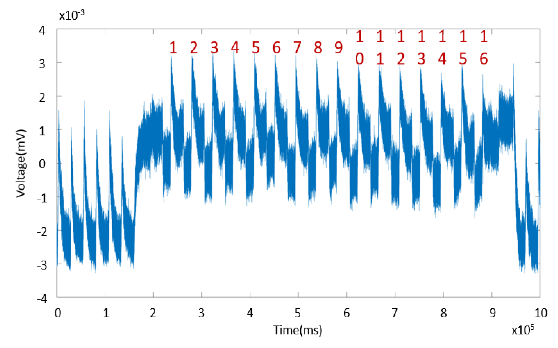
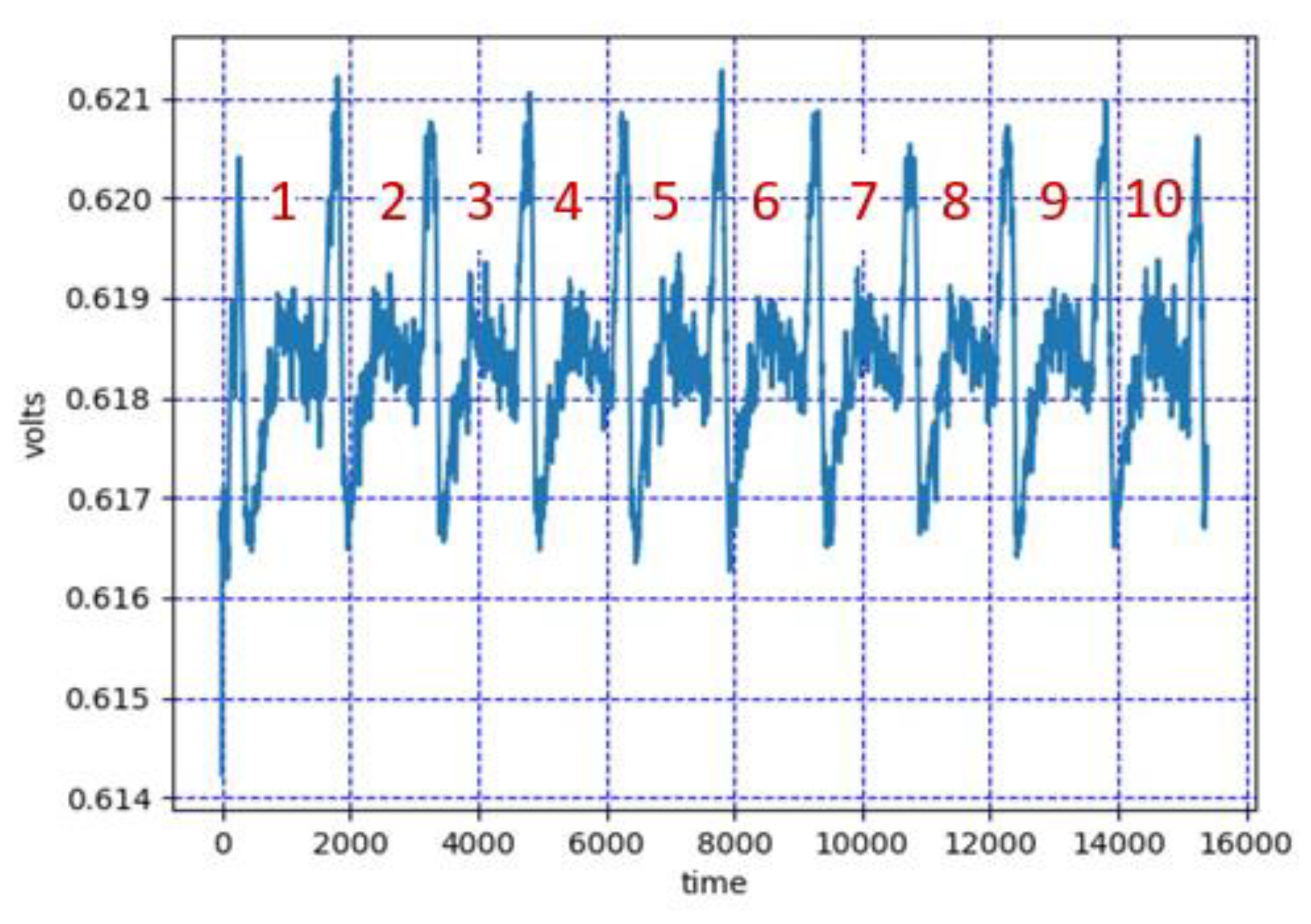
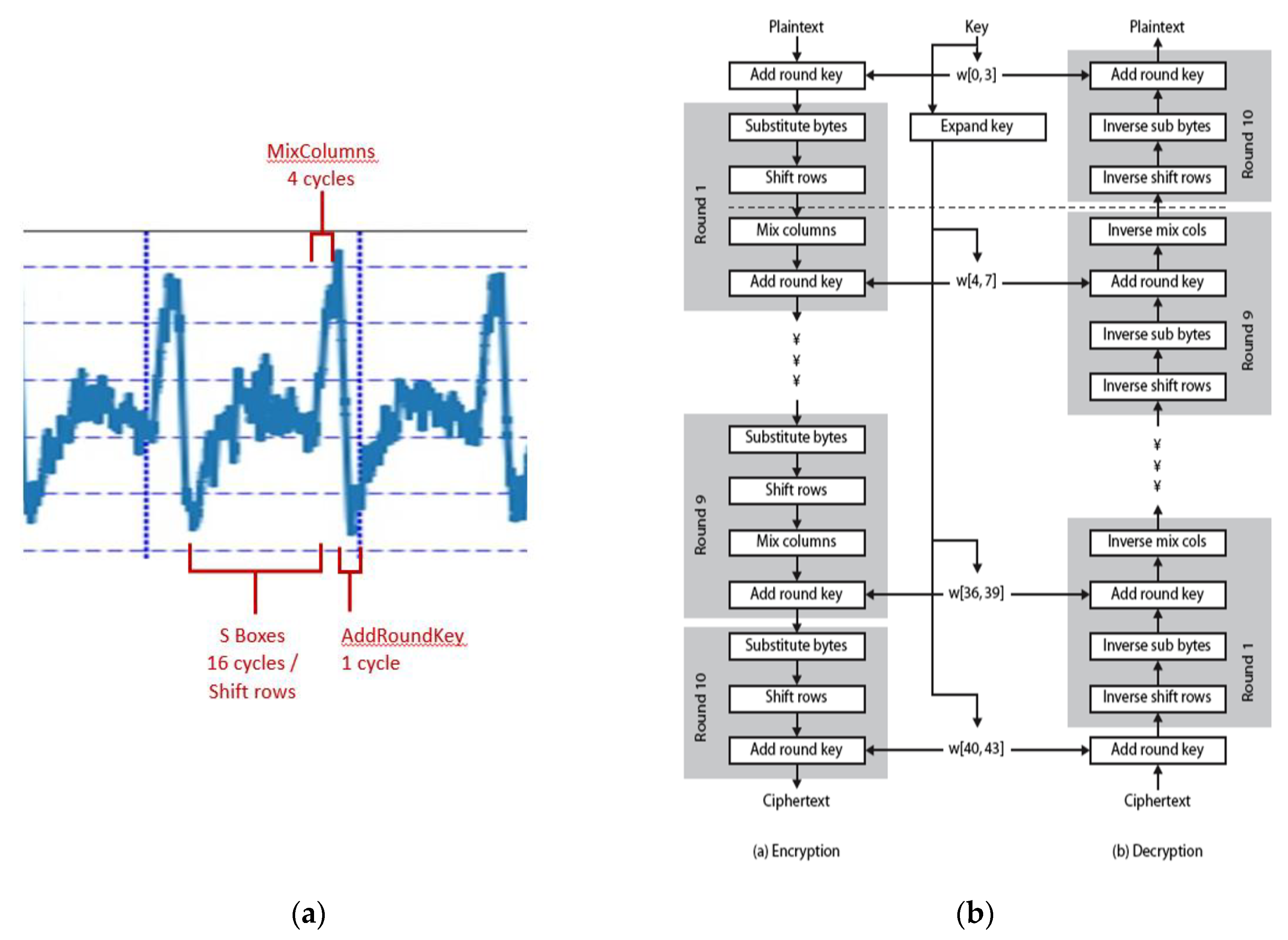
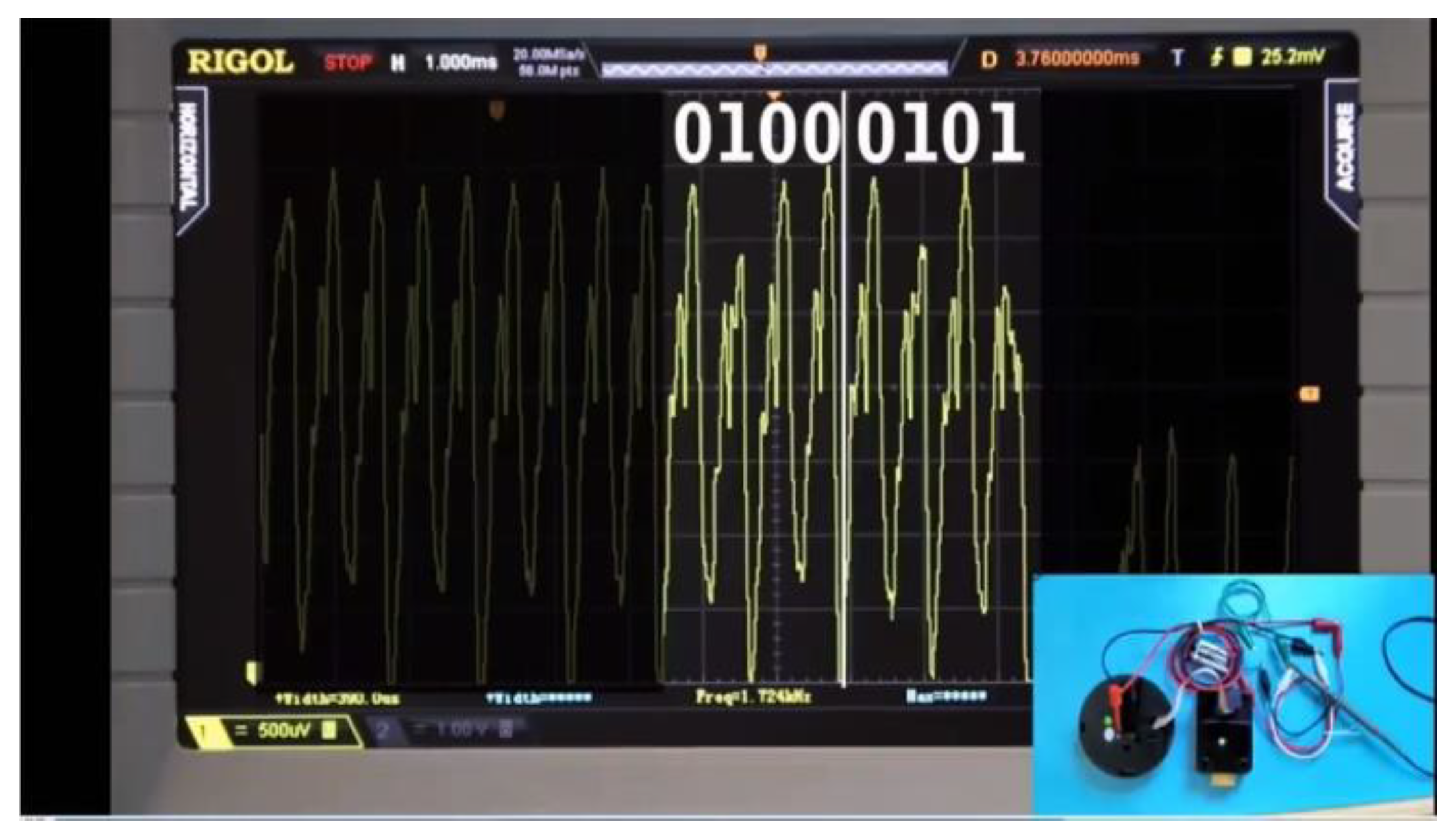
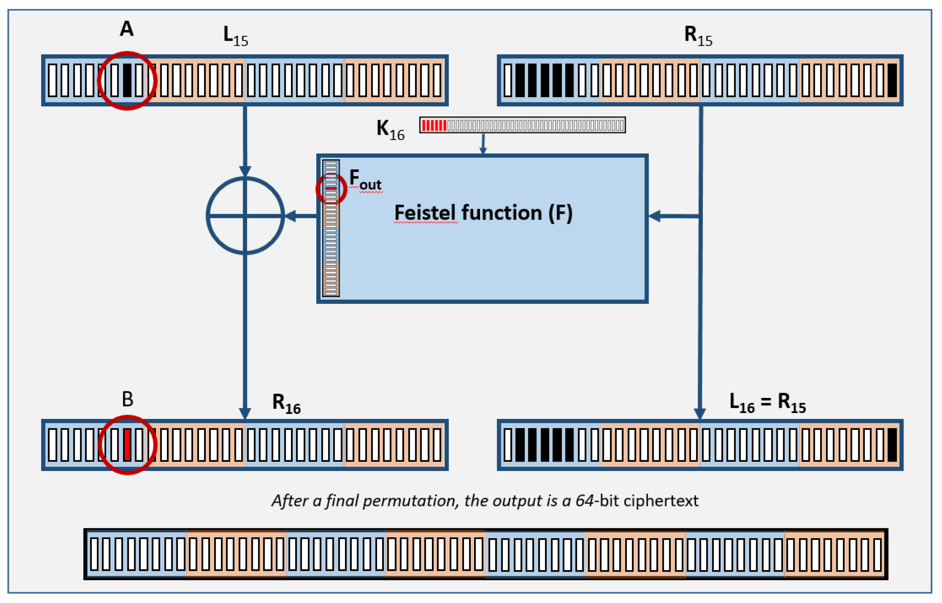
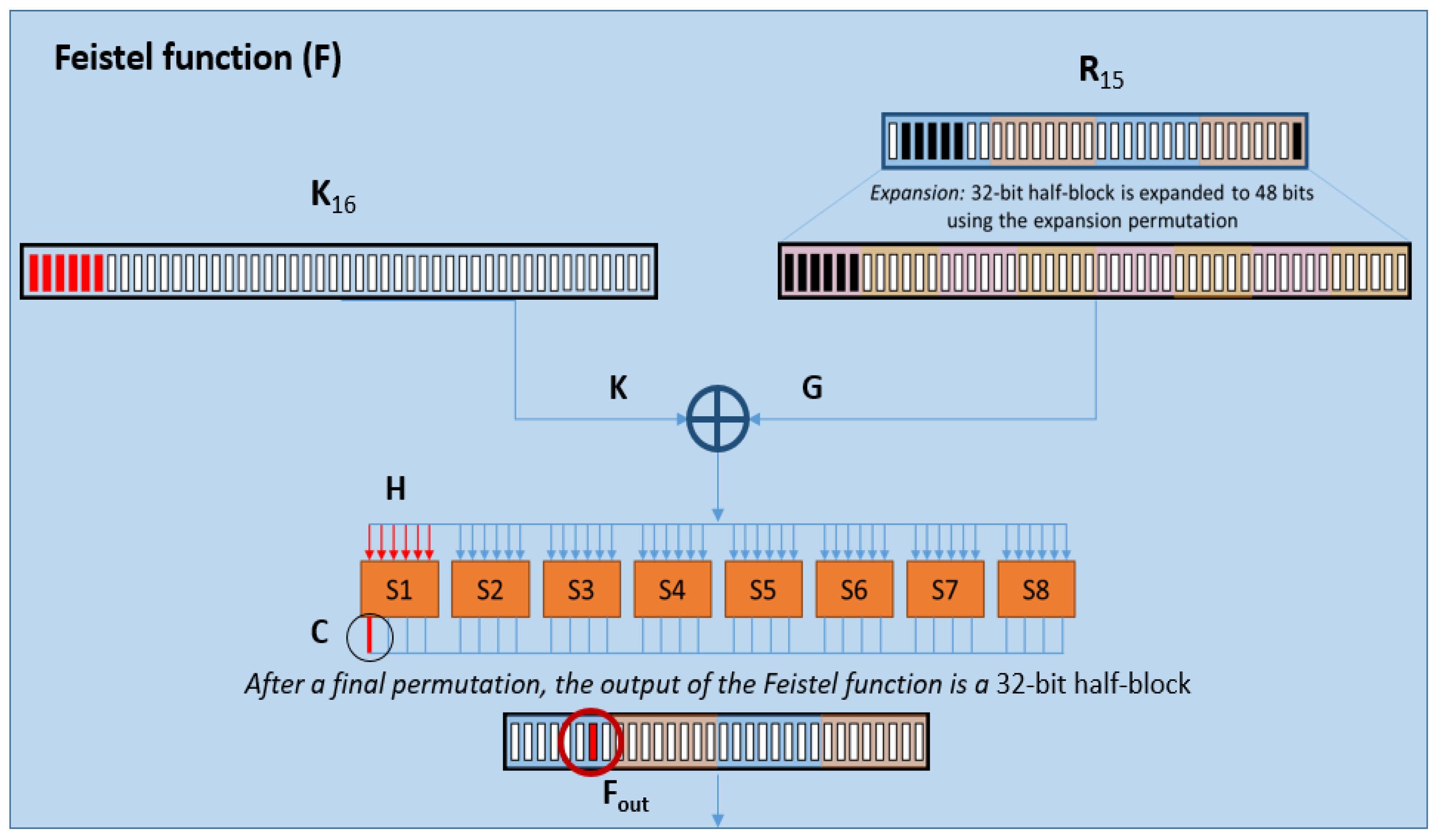
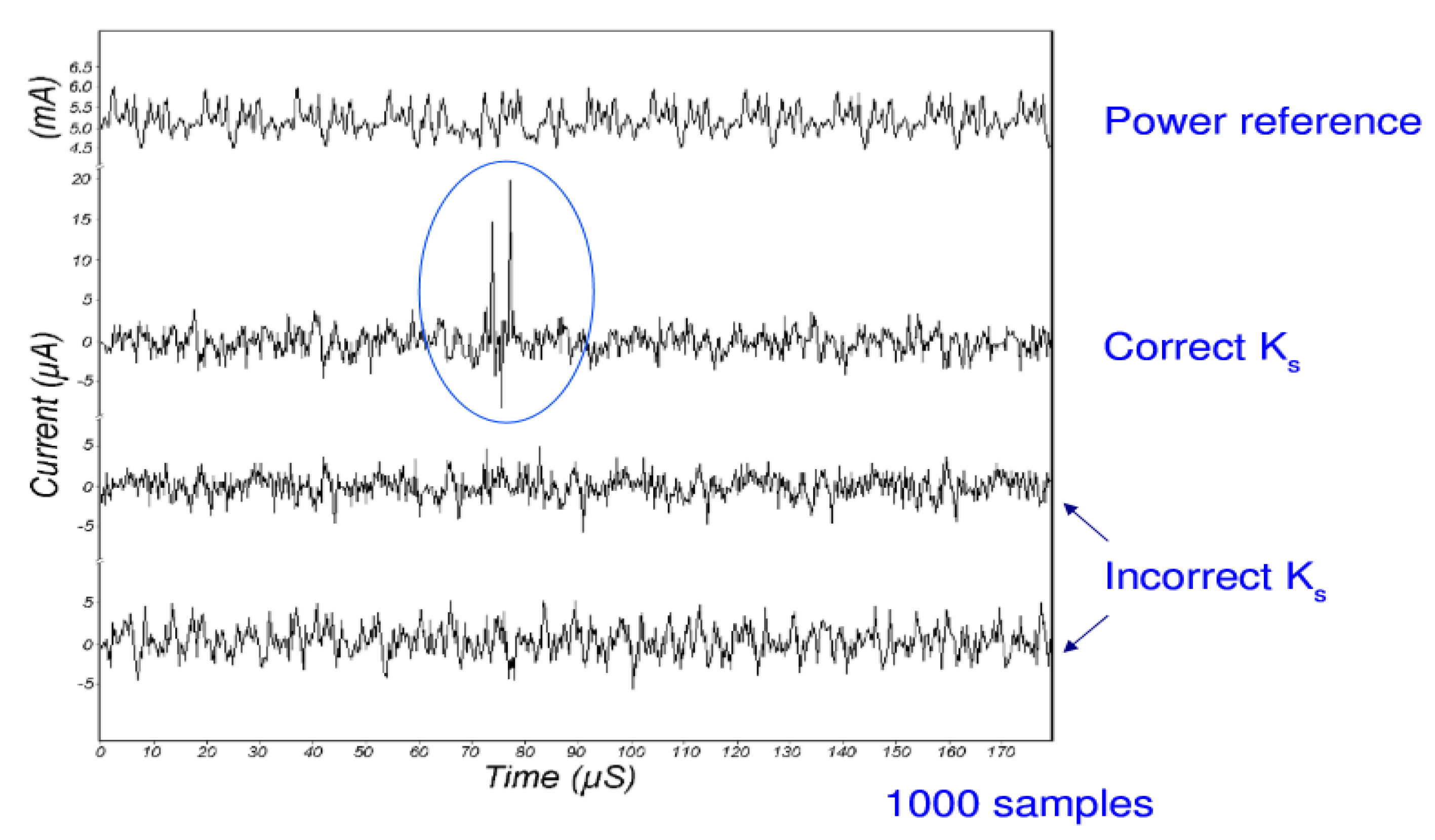
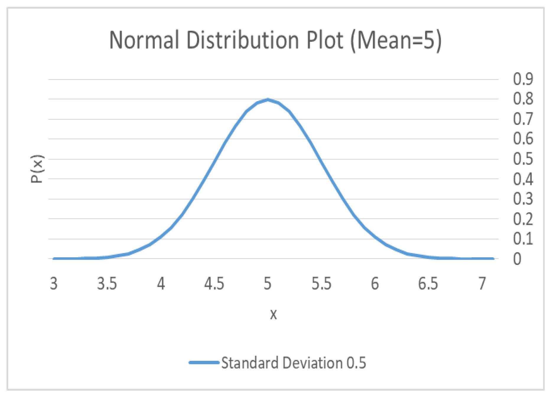
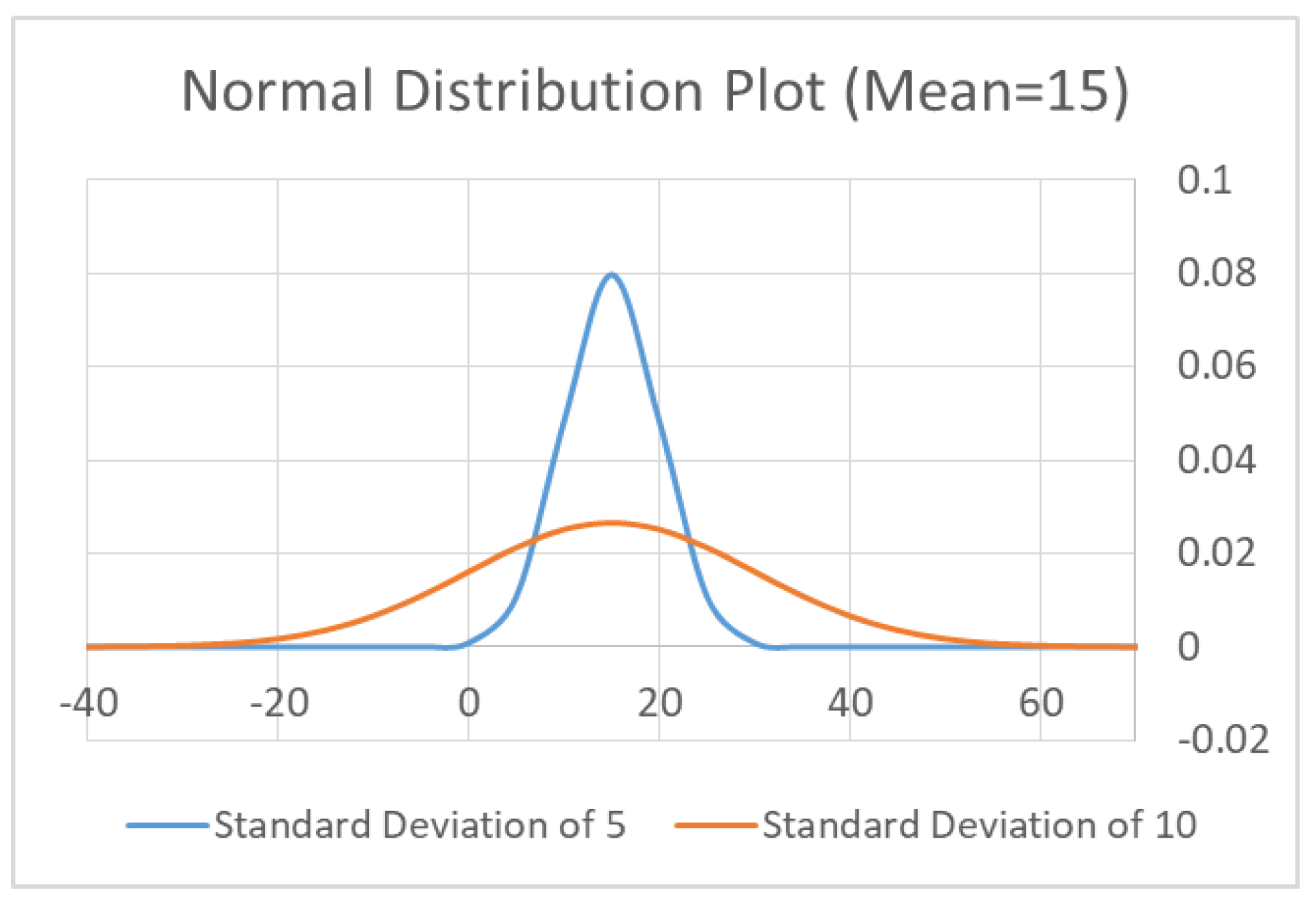
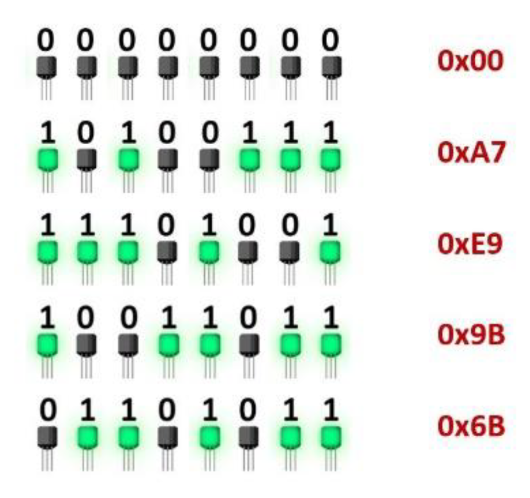
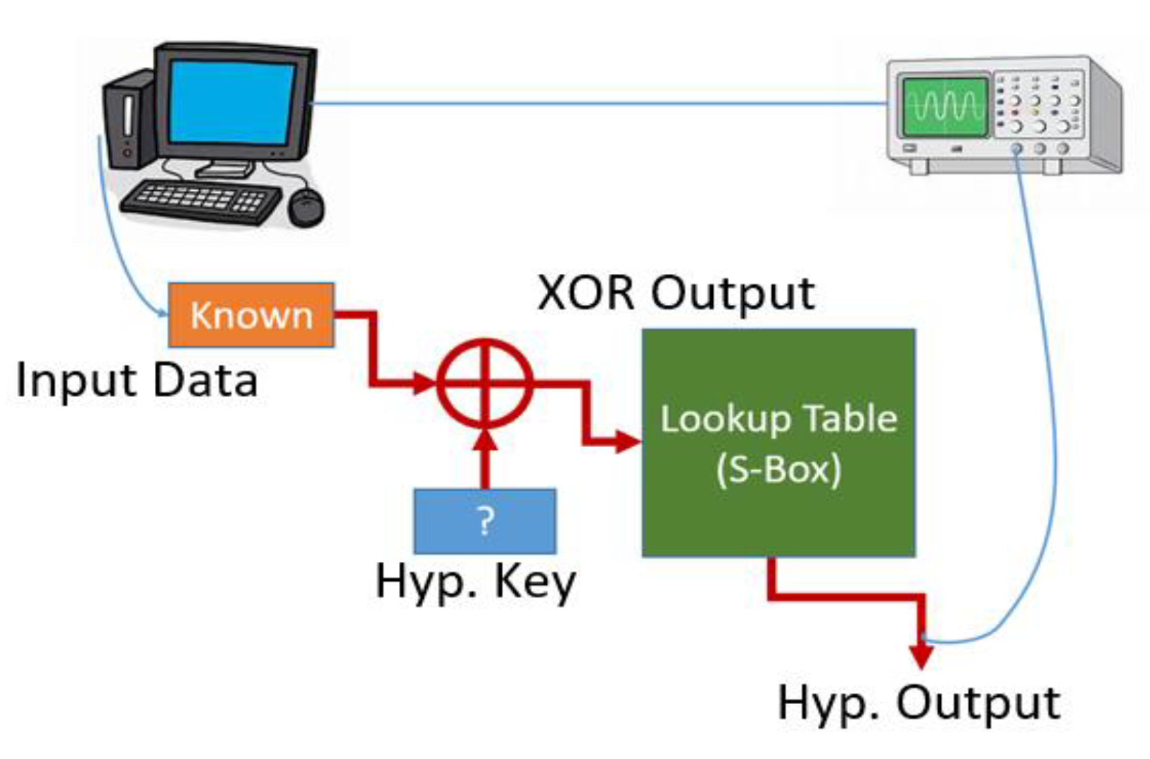
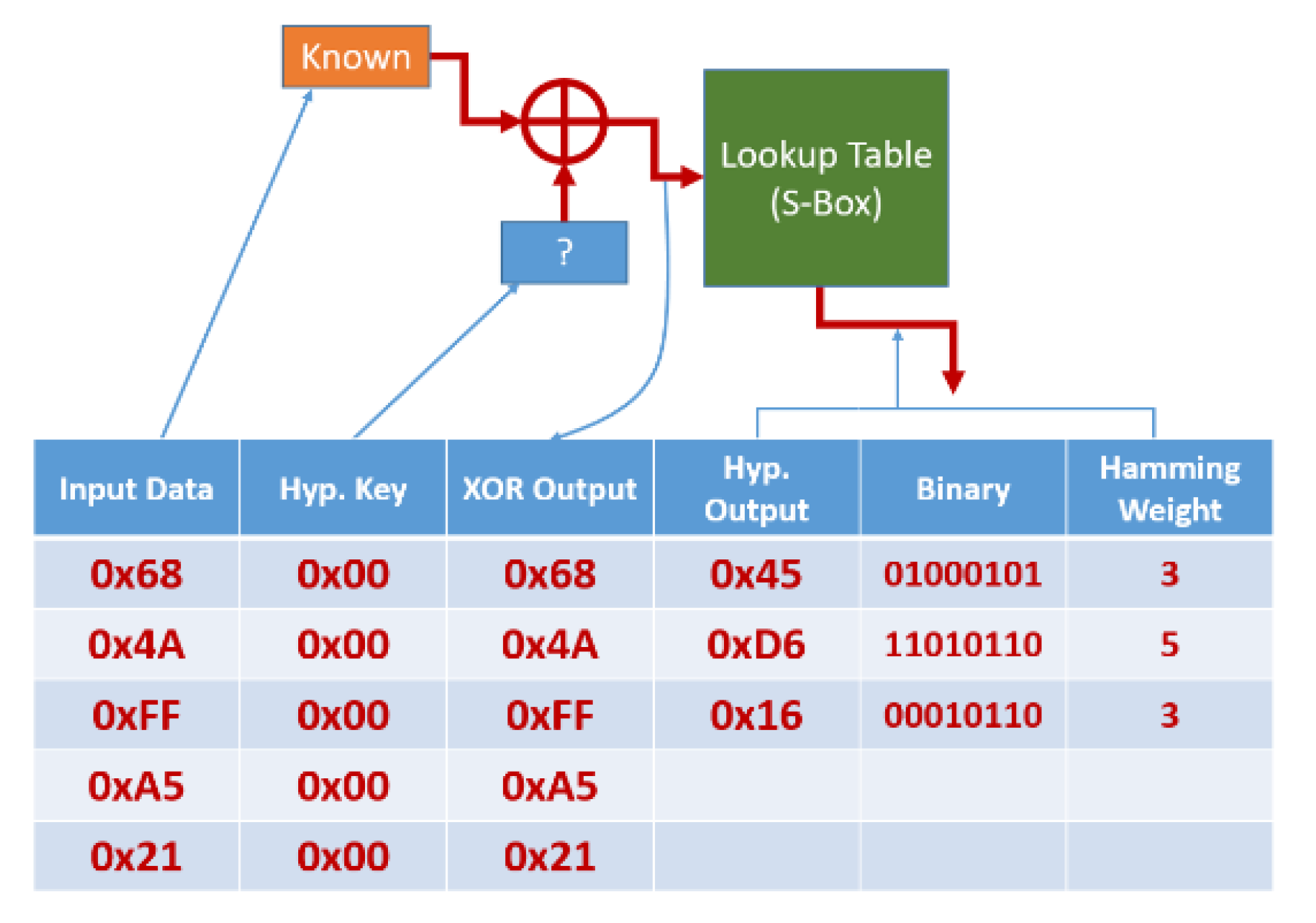
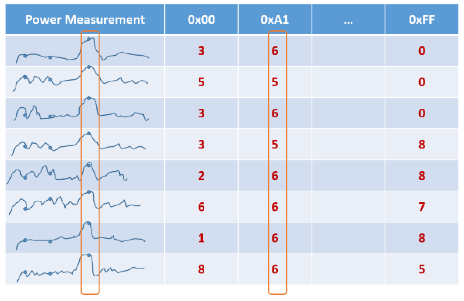
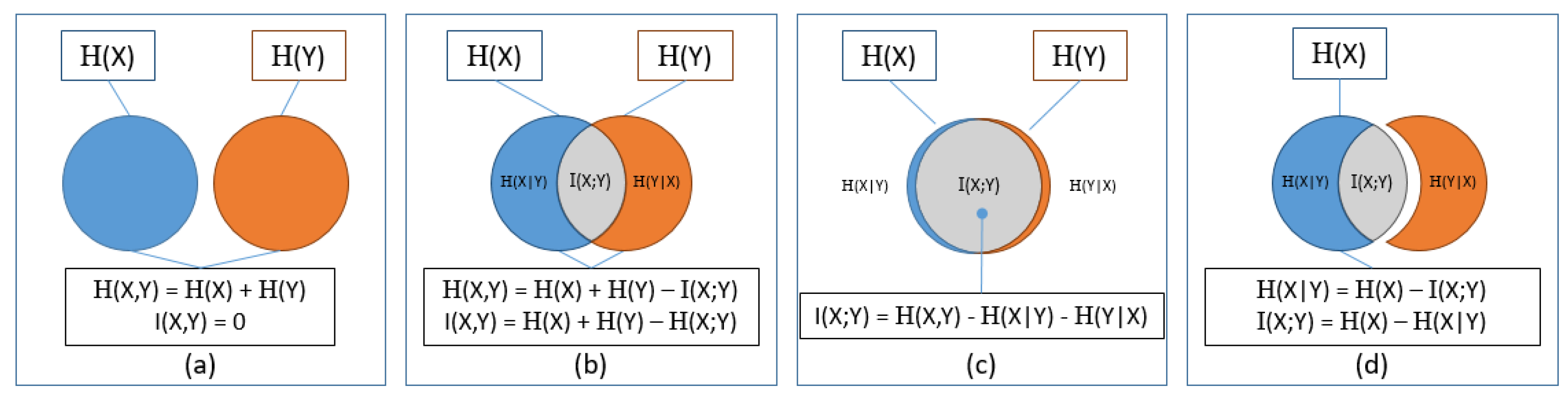
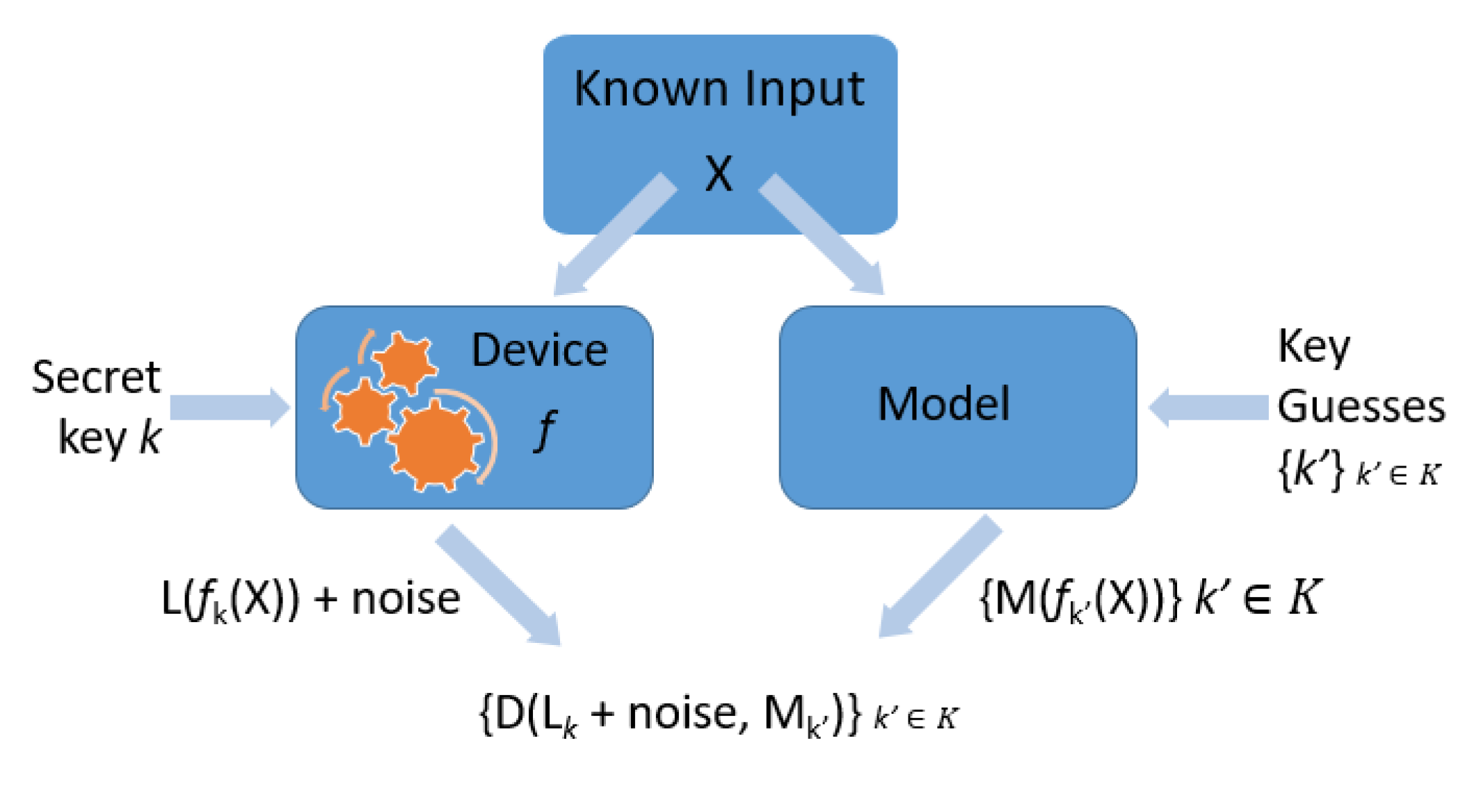
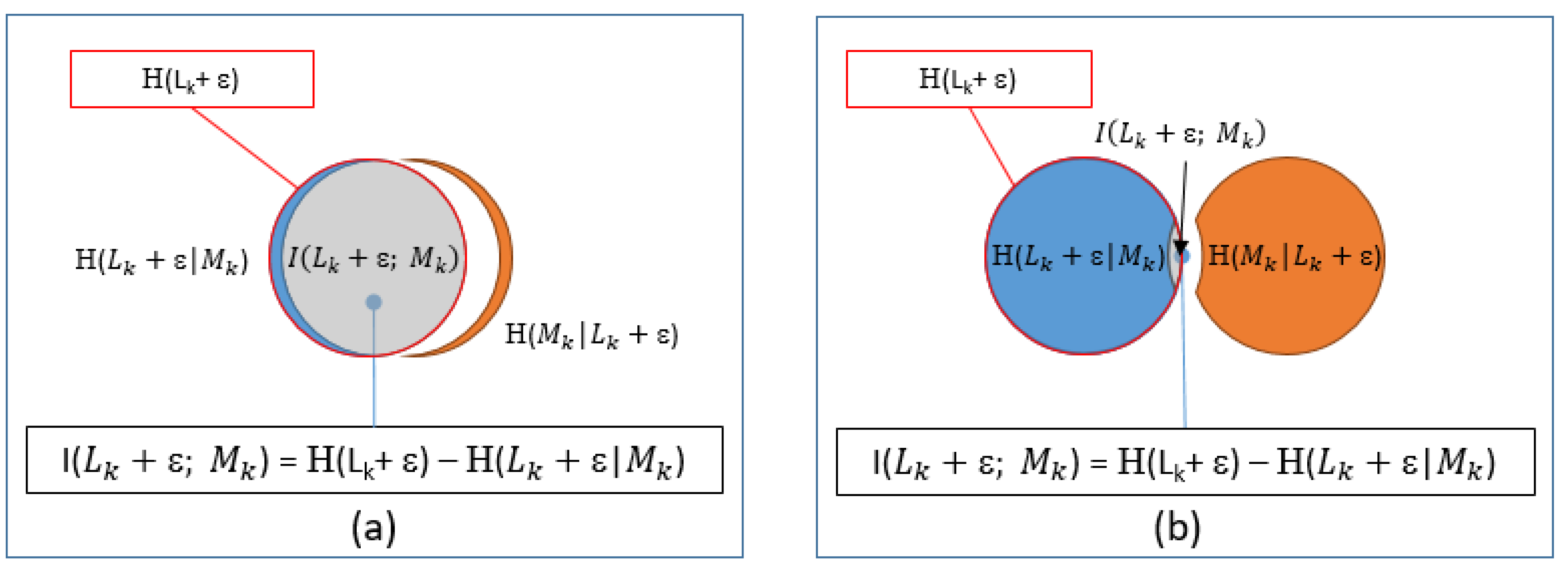
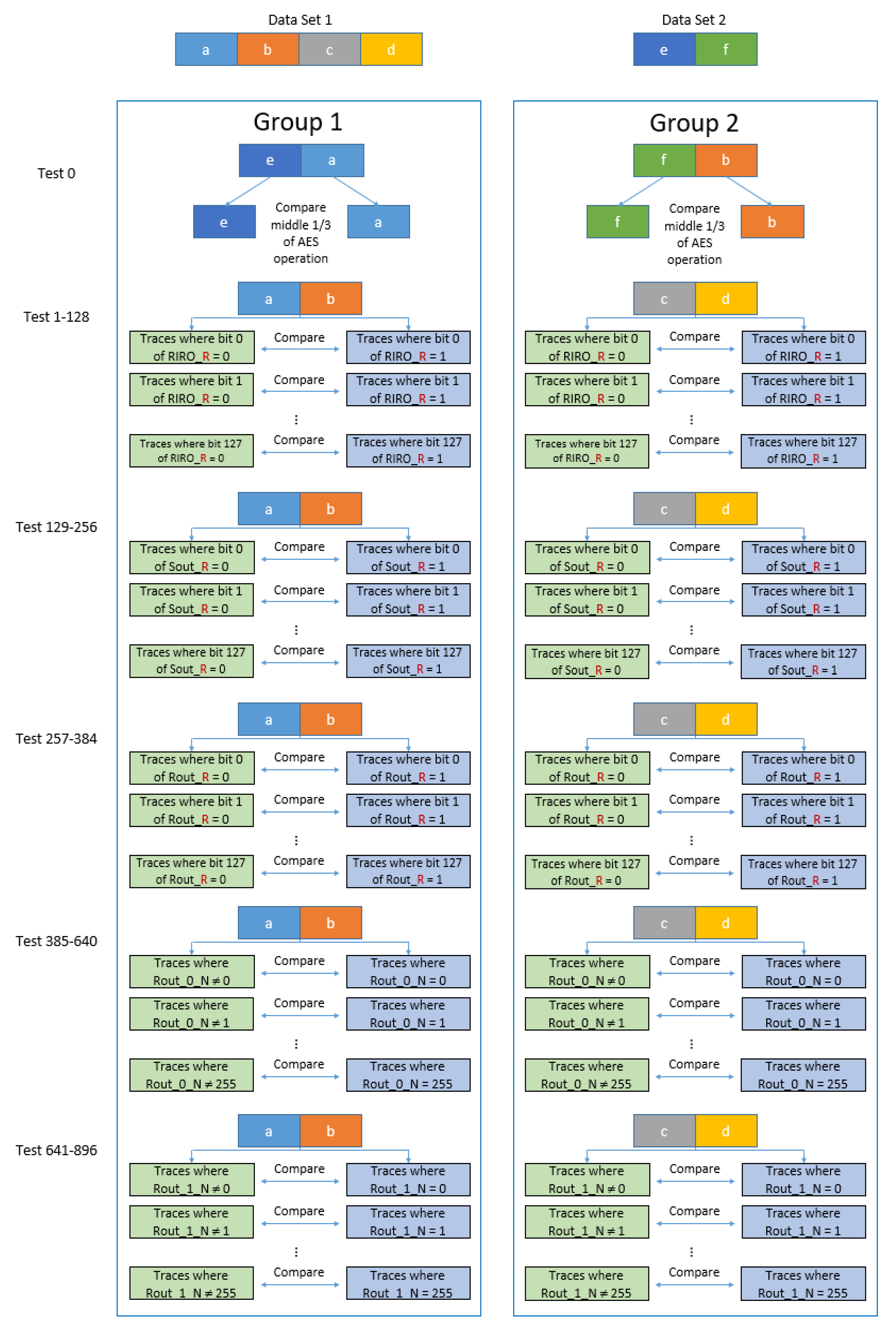
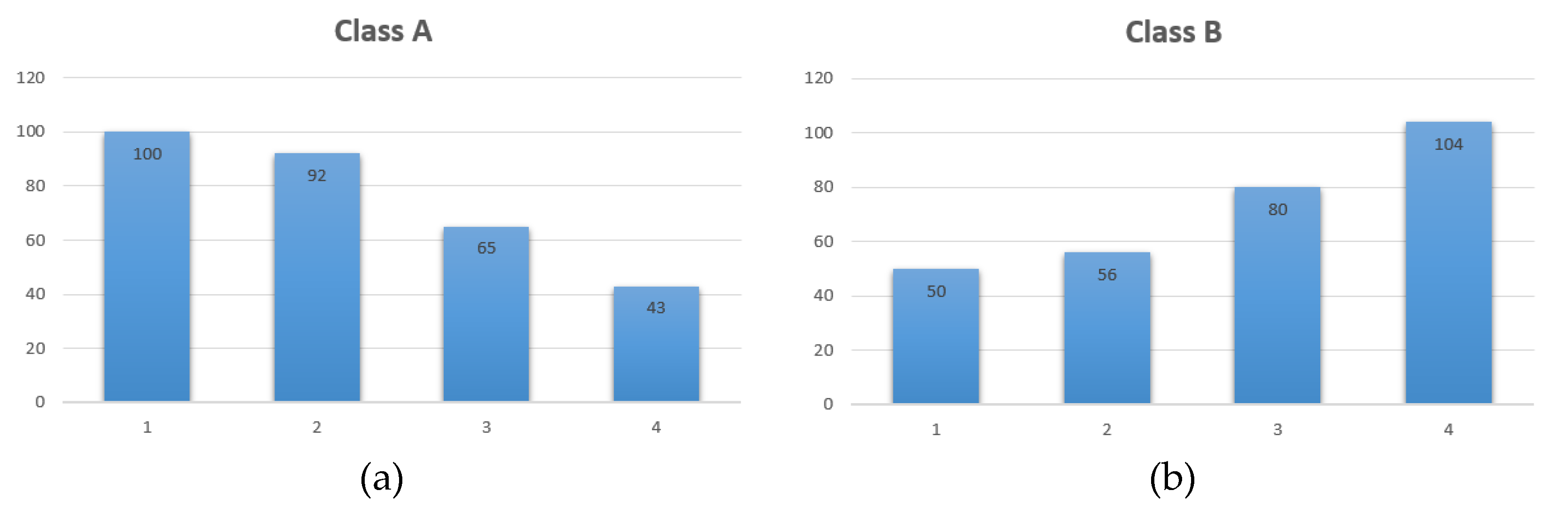
Table 1.
Contingency table for two example sets of data.
| Fi,j | j = 0 | j = 1 | j = 2 | j = 3 | Total |
|---|---|---|---|---|---|
| i = 0 | 100 | 92 | 65 | 43 | 300 |
| i = 1 | 50 | 56 | 80 | 104 | 290 |
| Total | 150 | 148 | 145 | 147 | 590 |
Table 2.
Expected values for two example sets of data.
| Eij | j = 0 | j = 1 | j = 2 | j = 3 |
|---|---|---|---|---|
| i = 0 | 76.27 | 75.25 | 73.73 | 74.75 |
| i = 1 | 73.73 | 72.75 | 71.27 | 72.25 |
© 2020 by the authors. Licensee MDPI, Basel, Switzerland. This article is an open access article distributed under the terms and conditions of the Creative Commons Attribution (CC BY) license (http://creativecommons.org/licenses/by/4.0/).
Share and Cite
MDPI and ACS Style
Randolph, M.; Diehl, W. Power Side-Channel Attack Analysis: A Review of 20 Years of Study for the Layman. Cryptography 2020, 4, 15. https://0-doi-org.brum.beds.ac.uk/10.3390/cryptography4020015
AMA Style
Randolph M, Diehl W. Power Side-Channel Attack Analysis: A Review of 20 Years of Study for the Layman. Cryptography. 2020; 4(2):15. https://0-doi-org.brum.beds.ac.uk/10.3390/cryptography4020015
Chicago/Turabian StyleRandolph, Mark, and William Diehl. 2020. "Power Side-Channel Attack Analysis: A Review of 20 Years of Study for the Layman" Cryptography 4, no. 2: 15. https://0-doi-org.brum.beds.ac.uk/10.3390/cryptography4020015