
Improved Filtering Techniques for Single- and Multi-Trace Side-Channel Analysis


1
Faculty of Engineering, Bar-Ilan University (BIU), Ramat-Gan 5290002, Israel
2
Department of Electrical Engineering and Computer Science, Massachusetts Institute of Technology (MIT), 77 Massachusetts Avenue, Cambridge, MA 02139, USA
*
Author to whom correspondence should be addressed.
†
These authors contributed equally to this work.
Cryptography 2021, 5(3), 24; https://0-doi-org.brum.beds.ac.uk/10.3390/cryptography5030024
Submission received: 14 August 2021
/
Revised: 3 September 2021
/
Accepted: 4 September 2021
/
Published: 13 September 2021
(This article belongs to the Special Issue Implementation and Verification of Secure Hardware against Physical Attacks)
Abstract
:Side-channel analysis (SCA) attacks constantly improve and evolve. Implementations are therefore designed to withstand strong SCA adversaries. Different side channels exhibit varying statistical characteristics of the sensed or exfiltrated leakage, as well as the embedding of different countermeasures. This makes it crucial to improve and adapt pre-processing and denoising techniques, and abilities to evaluate the adversarial best-case scenario. We address two popular SCA scenarios: (1) a single-trace context, modeling an adversary that captures only one leakage trace, and (2) a multi-trace (or statistical) scenario, that models the classical SCA context. Given that horizontal attacks, localized electromagnetic attacks and remote-SCA attacks are becoming evermore powerful, both scenarios are of interest and importance. In the single-trace context, we improve on existing Singular Spectral Analysis () based techniques by utilizing spectral property variations over time that stem from the cryptographic implementation. By adapting overlapped- and optimizing over the method parameters, we achieve a significantly shorter computation time, which is the main challenge of the -based technique, and a higher information gain (in terms of the Signal-to-Noise Ratio ()). In the multi-trace context, a profiling strategy is proposed to optimize a Band-Pass Filter (BPF) based on a low-computational cost criterion, which is shown to be efficient for unprotected and low protection level countermeasures. In addition, a slightly more computationally intensive optimized ‘shaped’ filter is presented that utilizes a frequency-domain -based coefficient thresholding. Our experimental results exhibit significant improvements over a set of various implementations embedded with countermeasures in hardware and software platforms, corresponding to varying baseline levels and statistical leakage characteristics.
1. Introduction
Side-channel analysis (SCA) attacks over cryptographic implementations are constantly evolving and improving. Current and future primitives and their implementations are designed to enable low-cost embedding of security mechanisms as much as possible [1,2]. However, new channels and adversarial mechanisms are constantly on the rise; for example screaming channels [3] that target Radio Frequency (RF) ID IoTs, multiple-SOCs/Network/cloud SCAs, e.g., [4,5,6,7,8,9], which are directed towards more general computing platforms, to name a few. Future Lightweight Crypto. and Post-Quantum Crypto. proposals are nowhere near to a solution to the side-channel issue with respect to the low electronic cost requirements of countermeasures. In particular, information extraction and exfiltration mechanisms provide leakages with different statistical characteristics. For example, the electromagnetic channel provides leakages with less algorithmic noise which are more sensitive to specific frequency ranges. Information sniffing over multi-process computation platforms shape different characteristics of the leakage due to the characteristics of these SCA channels; e.g., through on-chip sensors or analog-to-digital converters (ADCs). Therefore, preprocessing and denoising tools and abilities must be improved and adapted to evaluate worst-case leakage scenarios.
In this paper, we address two scenarios. The first, denoted as the single-trace context, depicts a scenario in which an adversary has access to only one leakage trace, e.g., corresponding to one encryption (or only a few traces). This scenario is applicable when very frequent re-keying takes place, or other randomization mechanisms exist. This scenario is particularly important in the context of asymmetric protocols and horizontal attacks [10,11]. The second scenario refers to the multi-trace (or statistical) context, and corresponds to the classical SCA attack context where an adversary has access to numerous measurements. This scenario is highly applicable to symmetric protocols. Both scenarios are of interest, and will continue to be subjected to adversarial activity.
Filtering techniques are utilized in both the single- and multi-trace scenarios. For the two, the SCA literature tends to suggest heuristic optimization techniques to pre-process the traces and reduce the noise or filter the raw traces. There are many meta-parameters including the bandwidth and frequency ranges of a filter, its shape, and the domain it is manipulating [12,13,14,15,16,17] (e.g., time, frequency or other domains, such as the wavelet domain [15,18]). Filters are utilized extensively in the field and in particular in the side-channel related literature. However, experimentation or reports typically only deal with one ad hoc chosen filter. Thus, to the best of our knowledge, different filters have not been compared and analyzed in a systematic fashion. Stated differently, filters have never been concretely compared with respect to an optimization criterion from the SCA security context with a clear holistic approach. Nevertheless, this type of approach has promise since it can lead to sharper conclusions in the quest to find the ‘best’ filter for this specific purpose. These efforts should also be complemented by an informative metric, to enable an accurate quantitative comparison to a simple or trivial filter.
Most attacks and widespread security analyses, especially on low-cost countermeasures (simple power randomization, flattening countermeasures, shuffling, etc.) are naturally univariate when low computational complexity is desired. For example, although it is well known that a multivariate analysis would be the most effective approach to extracting information from a shuffled design, typically a univariate analysis is utilized subsequent to a tailored filter such as convolution with a window function or averaging to combine the different leakages stemming from a shuffled set of time samples. This underscores the need to analyze and compare different filtering techniques focusing on such univariate adversaries. This manuscript thus addresses the potential gains while using an optimization criterion to devise the best (in some well-defined sense) filter. In addition, we explore a set of different cryptographic implementations embedded with countermeasures, where each provides different leakage characteristics; in turn, these different characteristics exemplify whether these optimized filters respond better than other more naive filters.
Another frontier, which is much less theoretically analyzed or experimented with, is the single-trace context. Statistical noise reduction techniques utilized in the single-trace scenario, such as Singular Spectral Analysis [19] (SSA), mostly serve heuristic single-spectrum thresholds and evaluation techniques to exclude noise components. In this work, we extend the original proposal [20], which is adapted to the SCA context. Our initial observations, supported by concrete demonstrations, is that most SCA leakages vary the spectrum characteristics of their leakage as a function of the time sample. These characteristics also behave differently when different countermeasures are examined, as discussed below. While considering this property, we utilize a technique of overlapped (OVSSA [21]) over a piece-wise constant spectral-characteristics time window. This approach produces considerably improved noise-removal capabilities, and perhaps more importantly, significantly reduces the processing time complexity, which constitutes the SSA/OVSSA bottleneck.
The main contributions of this paper are as follows:
- We improve upon the technique adapted to the single-trace SCA context by utilizing the variations in spectral properties over time. By implementing OVSSA [21], adapting it to the single trace scenario and optimizing over the method parameters, we achieve not only a significantly shorter computation time, which is the main Achilles’ heel of the method, but also lower the data complexity and generate an overall higher information gain (in terms of the Signal-to-Noise Ratio ()). Concretely, the proposed technique provides ∼5× max. improvement for about the same number of leakage traces (data complexity). However, the main improvement is in the pre-processing evaluation time. The based pre-processing technique time complexity depends primarily on a Singular Value Decomposition (SVD), which is generally quadratic in time as a function of the number of leakage time samples, n. The OVSSA based pre-processing technique time complexity depends on SVDs over chunked leakage traces (fewer samples), with a parameter Z, i.e., . That is, the time complexity improvement is generally , which was shown to be significant in our experiments. i.e., Z depends on the spectral characteristics of the leakage throughout the trace and for round-base cryptographic implementations the factor is expected to yield significant improvements.
- In the multi-trace SCA context, we devise a profiling tactic to optimize a Band-Pass Filter (BPF) based on a criterion utilizing a low computational cost metric in Section 2.4.3. Our experiments below achieve optimal results for unprotected designs. However, as the protection level increases, the (optimized) BPF shows a significant reduction in performance that can be attributed to the different and more complex spectrum of the leakage, which requires more sophisticated filters. Therefore, we also propose an optimized shaped filter utilizing a frequency domain -based coefficient thresholding for the multi-trace scenario. The results obtained when using this filter show significant improvements over all datasets and designs, yield the highest compared to all the other methods with an improvement of an order of magnitude, and reduce data-complexity by a factor of ∼2.5×, as reported in Table 1.
The rest of the paper is organized as follows. In Section 2, we present the low computational effort toolbox we chose to evaluate security, which is used in our proposed criterion for optimal filter design. In Section 2.3, we describe single-trace pre-processing techniques and possible improvements by adapting OVSSA Section 2.3.2, and in Section 2.4.3 we detail the multiple-trace (statistical) pre-processing techniques, while defining our optimization criterion and set of parameters that are optimized for band-pass filters and shaped filters. In Section 3, we present the designs and countermeasures from which we collected datasets to apply these tools. In Section 4, we describe the experimental results, and the data and complexity gains for both the single-trace and multi-trace scenarios in Section 4.1 and Section 4.2, respectively. Finally, a discussion of the results along with some concluding remarks are provided in Section 5.
2. Tools and Theory
In this section, we first discuss our optimization criterion for optimal filter design and our evaluation setting. We then describe in detail the single-trace and multiple-traces pre-processing techniques proposed in this paper.
2.1. A Simple, Computationally Attractive Optimization Criterion
In this subsection, we discuss the simple metric we use to evaluate security, namely the SNR, and present the rationale for this particular metric. We further detail the evaluation scenario; i.e., a profiling adversary, in the context of filter estimation (profiling), utilized in an attack campaign. Consider an internal variable manipulated by a cryptographic algorithm, Y of n-bit, and y its realization. Throughout the data manipulation by a device, information leaks via side-channels and is associated with the manipulated data, as well as with other physical parameters. We assume henceforth that an adversary takes a divide- and- conquer approach over a small chunk of a secret variable of bits, such that . Denote a leakage trace by a measurement set of T time points, . The leakage trace, corresponding to the manipulation of y, is therefore denoted by . A matrix of these leakage traces, containing a set of measurements of several realizations y, is denoted by L.
In what follows, we focus on a univariate analysis of the leakage distribution targeting one of the most widespread adversarial scenarios, which also enables a tractable analysis. Our main goal is to devise a simple security oriented metric that can be efficiently processed on the one hand, but on the other is sufficiently statistically robust to capture the main leakage characteristics of simple countermeasures embedded within a device. The rationale for this fast processing metric is our goal to utilize it as an optimization criterion for filters, which is why the procedure is repeated across multiple optimization parameters. Theoretically, there are scenarios which can be augmented by a multivariate analysis (or a multivariate leakage distribution over multiple leakage time samples jointly), e.g., when shuffling [22] or serial masking [23,24] countermeasures are embedded. However, in our measurement and evaluation environment, we evaluate a large set of different countermeasures that are almost all low-cost and univariate by nature. We address several basic questions concerning optimal filtering with varying leakage distributions. We also use the univariate approach in the shuffled leakages scenario, though a very complex multivariate approach could be applied [22], albeit with exponential data complexity in the number of dimensions. This is due to the fact that the univariate approach is still indicative of the level of leaked information from a shuffled design.
The SNR is a statistical measure that indicates how informative a signal is within a noisy environment: it compares the power level of a signal to the power level of the background noise; hence, the assumption is that the evaluator has access to labeled leakages. Traditionally, the SNR is defined as the ratio of the signal power to the noise power. in the side-channel sense, as first proposed by Mangard [25]. The SNR has been utilized in numerous works and aims to indicate the univariate informativeness of a leakage time sample. To do so, both the signal and noise components are estimated. The signal power is estimated by first averaging out the noise in the leakage per secret variable state (y), and then computing the outcome-leakage variance over y. The noise first captures the level of noise (variance) in the leakage per y state, and averages the outcome-leakage over the states. Specifically, for the t-th leakage trace, the SNR defined by
Of course, in practice, the true quantities in Equation (1) are unknown, so that we use estimates (using empirical averages and standard deviations) to obtain an estimate of the SNR. In the evaluation cases below we target y, giving , where x and k are the plaintext and key, respectively, and is the substitution-box step taking place in the first round of the advanced encryption standard (AES) algorithm implemented within our encryption cores.
Note that although the univariate SNR makes use of simplifying statistical assumptions regarding the leakage distribution, it is still probably the most widespread and viable tool to identify points-of-interest (POI) in time where the manipulation of a secret variable takes place, and is also used to link higher level security estimations such as the guessing entropy (GE) or the attack success rate (SR). In addition, it typically serves as a tool for valuable speedup of security evaluations. Generally, information-theoretic-based metrics, such as the ones used in [26,27], and full distribution analysis would be more statistically correct to use. However, in the context of this particular work, they are less practical for performing fast calibrations of many filter parameters due to their high computational complexity and their underlying data complexity, which are required to fully capture the leakage distribution.
2.2. A Profiled Evaluation
Template attacks [28] are performed in two subsequent (or interleaved) phases of profiling and attack. It is assumed that the adversary has gotten hold of one device for which the secret key can be programmed (in a controlled manner), so that the leakage can be profiled. Then, another target device under an attack campaign is used, where the adversary tries to extract information on the underlying key. In the context of a multi-trace (statistical) scenario, where we aim to find a viable filter, we consider the template setting; namely, we assume the leakages are y-labeled to optimize the w.r.t. filter parameters.
2.3. Single Trace Techniques
2.3.1. Utilized for SCA Denoising
is a spectral estimation method, which is utilized in classical time series analyses, multivariate statistics, multivariate geometry, dynamic systems analysis and signal processing [29,30,31,32,33,34]. can be applied to a single trace (i.e., it requires a single vector observation, denoted by one measurement here). can serve to decompose a signal into meaningful components (usually divided into trends, oscillations, and noise) relying on the celebrated SVD, which can be used for denoising. In our context, can be applied as a pre-processing tool to each measurement (time series measurement). Then, the estimated , based on a set of single processed measurements, can be utilized to evaluate the gain in the security context. The feature of interest in this case is the ability to reduce noise with SSA, as was successfully demonstrated in [20]. Formally, denote , a time series measurement (leakage trace), and further, define the matrix as
where K defines the window length of observations in X, allocated to each row of the matrix. From the first row, each following row is skewed by one sample. The number of rows, L, is set from N by the selection of the window size K, i.e., . is a general case of a “non-square Hankel matrix”. A Hankel matrix is a square matrix in which each ascending skew-diagonal from left to right is constant.
The procedure follows the computation of the (unnormalized) sample covariance matrix , where represents the transposition, computing the (non-negative) eigenvalues of , denoted by , and sorting them in a decreasing order, where represent their corresponding eigenvectors. Then, compute , while keeping only a subset eigenvectors which are associated with the trend and oscillation components, and excluding ones associated with the noise components. That is, one needs to choose sets of indices , corresponding to a set of eigenvalues, where and are disjoint for all , and the union of all the sets sets is . Then, these sets are associated with the trends, oscillations and noise components. Once the set of indices associated with noise components is chosen, one can simply exclude them and compute: . This decision step is typically based on thresholding the slope of the sorted descending eigenvalues as discussed below, and is generally highly heuristic; it depends on various parameters such as the noise distribution, the characteristic of the signal, and the parameters K and N. Therefore, closed-form formulas for thresholds are challenging to achieve with high coverage.
Finally, in order to reconstruct a time series denoised leakage trace from the resulting matrix, a Diagonal Averaging () step is utilized. If is a Hankel matrix, can simply average over elements corresponding to indices on each diagonal line in the matrix to form the time series. Formally, for matrix , it is defined as
If is not a Hankel matrix, it can be Hankelized, utilizing the Hankel transform (e.g., consider [35]).
An illustrative example is shown in Figure 1. Figure 1c shows an encryption current measurement quantized with a 16-bit oscilloscope versus measurement time (in time samples). Clearly, the repetitive round-based iterations of the encryption process are visible within the leakage. Figure 1a shows the sorted descending eigenvalues of corresponding to one leakage trace after SVD over . Finally, Figure 1b shows reconstructed elements associated with trends noise and oscillations.
Intuitively, rapidly changing eigenvalues correspond to trends, while slowly changing eigenvalues correspond to oscillations. However, without additional, restricting assumptions regarding the signal model, it is generally unclear how to predict the decay rate (i.e., slow or fast) of the ordered eigenvalues. Therefore, there is no universal method for consistent separation of the corresponding eigenvectors. Thus, heuristic approaches have been proposed, which are only efficient to some extent. Here, we chose to classify the eigenvectors based on their maximum discrete derivative with respect to the eigenvalues index (or slope), and suggest two heuristic thresholds, denoted by , to classify the eigenvectors, as specified in Algorithm 1.
| Algorithm 1: Trends, oscillations and noise thresholds setting. |
 |
In order to find the optimal parameters , we first compute the over the ’ed traces, listed in the matrix , independently for each time instance t. We then focus on the maximal SNR, based on which the optimal parameters are chosen. Formally, this optimization is described as
Here, the matrix is the leakage metric of all recordings corresponding to y realizations, listed in a vector of labels (required for the procedure). Note that optimal thresholding for eigenvalue exclusion while reconstructing signals with SVD was investigated in [36]. Though there are some similarities, embedding and reconstruction, and SVD reconstruction are different. In addition, the threshold presented in [36] is only optimal under certain conditions—for the noise (i.e., white), the dimensions of the measurement, and the variance of eigenvalues—and is only guaranteed asymptotically. In the SCA context, in most cases, the noise is not white nor can we meet the rest of these conditions, especially the dimensions of the measurements in the single-trace context.
2.3.2. We Can Do Better with OVSSA
Typically, cryptographic computations generate a repetitive structure of the leakage as a result of the periodicity of the computation (e.g., rounds in an SPN or sponge stages and iterations in asymmetric protocols) and due to the periodicity of the clock strobe. However, the spectral characteristics vary over the time sections throughout the computation. This is because the leakage on the first (last) rounds changes abruptly between computations, which is not related to encryption, to (from) a periodic sequence of encryption computations. However, the crucial points in time, for a divide and conquer adversary that aims to extract leakages prior to large key diffusion, are typically situated exactly where the spectral characteristics change rapidly, in the final (resp. initial) rounds. For example, the encryption spectogram exhibits varying spectral characteristics over time within the leakage, as illustrated in Figure 2. Therefore, any attempt to estimate spectral characteristics from the entire signal will not accurately characterize each and every individual time section robustly.
In this paper, to the best of our knowledge, is proposed for the first time in the SCA context. is defined with parameters q for the overlap and Z for the computation interval, where n is the number of time samples, and l is the window length (see [21]), in our case, q = 100 and Z = 201. l is determined by , where is a small constant, and (see derivation [37] and its use in the SCA context [20]). The Z parameter was derived in our experiments by investigating the spectrograms (e.g., see Figure 2), and observing the rate at which the spectral characteristics changed, where q was set to be roughly for a good overlap width. We chose c to be 1.5 to reduce the run time. Figure 2 shows that the most energized frequency components change with time, and that the change roughly does not span more than 200 time samples. This is the reason for a Z value of 201 (for example). More concretely, we specifically evaluate the argument maximizing the objective criterion for each of the hardware/software designs outlined below:
where implies performing with a computation interval of Z.
2.4. Multiple Traces (Statistical) Techniques
2.4.1. Multi Trace—Evaluation Criterion in the Time Domain
Generally, it is understood that data are modulated into SCA leakage traces with carrier frequencies such as the system clock. The reason for filtering the leakage is to preserve the signal contribution from frequency ranges that are informative and exclude all other frequency bands which contribute noise. However, it is difficult to know the type of filter required in advance, since it depends on multiple factors such as the measurement setup, the underlying device and the digital system complexity and the embedded countermeasures. Typically, filters are found and reported by ad hoc experimentation (trial and error), and parameters are set without any clear selection criterion, or alternatively they are optimized by heuristic methods. For several examples of the large range of band-pass (BP) filters, see [12,13,14], low-pass (LP) filters were recommended in [13,15], high-pass (HP) filters in [16,17] and band-stop (BS) filters [14].
To filter traces in the frequency domain, the discrete Fourier transform (DFT) is computed over the leakages, using the fast Fourier transform (FFT) [38], an efficient computation algorithm of the DFT. The magnitude and phase of the DFT components encapsulates their contribution to the overall signal. In our context, DFT evaluation can be used to analyze the frequency component separately from the filter noise-contributing components, etc. FFT has been shown to be efficient to overcome different side-channel countermeasures such as phase/time randomization [39], and to reduce sampling complexity [40,41].
An example of a standard cosine wave DFT versus a leakage traces DFT of one unprotected simple AES encryption case is illustrated in Figure 3a,b, respectively. Even this simple example captures the fact that most of the information is concentrated in a specific frequency band, with varying amplitudes. In the following, we show the increased complexity involved in finding good filters when countermeasures are embedded.
In order to fit the best filter, one must evaluate all parameters jointly per target design, i.e., without any prior knowledge. We denote the filter parameter set by {}, and compute the of the filtered traces in the time domain for each parameter set realization. Each computation must be performed on the entire dataset (assume N traces with n time samples each). We aimed to assemble sufficiently large datasets to reach convergence in the (i.e., to capture an accurate estimate of the ). The goal was to obtain solid statistics and be able to compare the data complexity as well as levels. Generally, the complexity required to perform the fitting operation is as follows: = , where is , which is negligible.
Denote a BPF as: , where w is the width of the filter, and i is the offset (or Slice as illustrated in Figure 4a. The filter is applied in the frequency domain: . Let us now define the optimization procedure for a BPF utilizing the time-domain metric formally:
where denotes we apply over each leakage measurement in matrix independently (on each row).
2.4.2. Efficiency Metrics for the Multi-Trace Context
We start by listing our two main objective functions: (1) low adversarial data complexity (Data) and (2) high leakage informativeness or information leakage (InfLk). More specifically, we are interested in assessing the asymptotic value of our information leakage evaluation metric (here, the SNR) along with the data complexity when reaching its asymptotic value. We weight both factors equally where the cost of data complexity is evaluated by , where is the number of required traces to reach the asymptotic value. Our combined (Data · InfLk) efficiency scalar metric, , is therefore defined as
The above efficiency metric is evaluated throughout this manuscript with one exception, for shuffling countermeasures. Because information spreads across time samples as an outcome of instruction shuffling, instead of looking at , we evaluate the integration of the SNR across the shuffled time span, to approximately quantify the total informativeness. More precisely, we define
where is a parameter for the number of shuffled clock cycles of the internal variable y.
2.4.3. Multi Trace—Frequency Domain Optimization Criterion
For protected designs giving rise to signals that sparsely occupy the frequency band of interest, a simple BPF cannot pass all the dominant frequencies without transmitting much of the noise with it. For example, Figure 12 shows that in the leakage spectograms of several countermeasures, such as dual-rail and shuffling, there are more than one dominant frequency bands. Hence, a different approach is required. To this end, we directly selected the dominant frequencies by isolating the frequency coefficients and using the simple univariate metric in the frequency domain to filter for the informative ones. This makes it possible to shape the filter (as illustrated in Figure 4b).
Formally, define , which denotes the SNR computed in the frequency domain over the DFT coefficients of the traces. We then select a subset of the DFT coefficients, denoted , based on a predetermined threshold:
where is the threshold from which we take DFT coefficients, based on their value, relative to the maximal value.
In this context, it is interesting to consider wavelet (and other) signal decomposition methods. The discrete wavelet transform (DWT) [15,18] is the sum over the duration of both scaled and shifted versions of the wavelet function. In particular, it has several meta-parameters for decomposition such as the number of scaled versions and shifts, and the basis functions. DWT is associated with another step to find effective side-channel leakage filters known as multi resolution analysis (MRA), which is a recursive composition of low-pass and high-pass filters. The methodologies discussed in this paper can naturally extend to other transforms and coefficient domains to filter out the noise in the transformed domain using an efficient cryptographic criterion. However, we chose not to evaluate the wavelets transform because of its very large space of associated meta-parameters. Our goal here was to target low-computational complexity optimization and fast evaluation. For slow but more complete approaches, one can also pursue information-theoretic based metrics, e.g., [26,27].
3. Designs and Datasets
In the experimental section below, we evaluate several different countermeasures leading to leakages with very different statistical characteristics, frequency domain characteristics, noise levels (on both hardware (HW) and software (SW) platforms), hence with different dataset sizes. Specifically, we evaluate the leakages captured from a:
- CMOS, 65 nm ASIC (HW)—unprotected rolled implementation of the AES (one round per clock cycle);
- Amplitude Randomization, 65 nm ASIC (HW)—protected by hardware amplitude randomization technique. Rolled implementation of the AES;
- Dual-Rail, 65 nm ASIC (HW)—protected by gate level flattening (WDDL implementation of Dual-Rail). Rolled implementation of the AES; and
- Shuffling, 40 nm Atmel 8-bit processor (SW)—protected by various instructions shuffling flavors: randomly permuting all groups of consecutive instructions (denoted in the following by , respectively;
The baseline (no pre-processing) level, #traces available, the protection mechanisms and platforms (SW or HW) are listed in Table 2.
4. Experimental Results
We analyzed the information gain and the data complexity of various design implementations of , and suggest improvements to existing methods. We addressed two contexts: multi-trace, and single-trace. In each context, our goal was slightly different. In the multi-trace context, we aimed to achieve the highest with the given toolbox (i.e., filters), while simultaneously reducing the data complexity as much as possible. In the single-trace context, we tried to achieve the highest possible while efficiently processing the data (i.e., maintaining low computational and time complexity) using only a single trace. Before discussing the experimental results, we refer the reader to Table 3 for a legend of the methods and naming conventions discussed in Section 2.
4.1. Multi-Trace
The most natural filter to utilize is a BPF given its simplicity and widespread use in the community. Our goal was to fit the best BPF to the data. Intuitively, the leakage of information from a device should only have a few dominant frequencies, since, for instance, outputs of the Sboxes are computed once per round, and each device leakage is modulated by a certain operation frequency (i.e., the clock frequency). Note that this is true for an unprotected design, but might not be valid for protected designs with, for example, randomized phase or complex analog-nature countermeasures (e.g., consider the shuffling case in Figure 9). Our goal was to more formally devise a rigorous procedure to evaluate various bandwidths (w) and offsets (i) empirically, and fit a different BPF on each hardware design. Based on the optimization procedure discussed in Section 2.4.1 we evaluate as shown in Figure 5).
The optimization of the threshold decision and the bandwidth and offset parameters are visualized in Figure 5: Figure 5a demonstrates that setting the threshold too low (too many frequencies) or too high (too few frequencies) results in a decrease in the of the filtered frequencies. Figure 5b demonstrates that there is one zone (from 500 to 600 in the DFT coefficients, roughly) in which the informativeness (evaluated via ) resides, where the optimal width is located in the ‘dense’ region of the graph. Notice that as the bandwidth increases, the graph becomes sparser. This is due to the fact that as the bandwidth increases, there are fewer frames. The parameter optimization results (CMOS) were: bandwidth (w) = 56 and offset (i) = 588 DFT coefficients, corresponding to 40 and 420 MHz, respectively.
Though the initial results were good; that is, the optimization process as compared to the results from the raw leakages showed significant gains, we predicted that the optimized BPF approach would not adapt well to more protected designs. Therefore, instead of trying to fit the best BPF filter, we turned to the shaped filter approach, which involves selectively keeping frequency coefficients, which are informative by using a metric to evaluate them, as discussed above.
For this purpose, a thresholding optimization procedure was defined in Section 2.4.1 to determine whether to include a certain frequency coefficient by evaluating its magnitude against the maximum value across all coefficients. The outcome filter obtained by choosing all informative frequencies formed a custom filter devolved to each of the designs/data sets/countermeasures embedded, a shaped filter (see Figure 6). This step resulted in a very significant impact on both data-complexity and extracted signal level.
With both methods in mind, we tested various designs and implementations. In Figure 6, the first row of the sub-figures shows a visual representation of the filters, the second row shows the corresponding of the optimal filters applied to the data sets; in other words, the optimal BP and the optimal shaped filter, as defined in Equations (6) and (9), respectively. As can be seen, the optimal BP-filter worked well for unprotected designs (e.g., unprotected CMOS), but failed to keep up as the design became more protected; e.g., for dual-rail and shuffling. The shape of the filter is rather interesting: for unprotected CMOS, we only observed one frequency cluster matching the optimal BP-Filter. For dual-rail, there were at least two main clusters, which are due to the fact that this design leaks at two carrier frequencies relating to the complete precharge phase (Return To Zero, RTZ) and evaluation phase. For the exemplary Shuffling test case, there are a few dominant frequencies, one of which is the clock of the micro-controller, and the others are a direct result of the shuffling operation: the Sbox computation can occur at two points in time, hence at several different frequencies.
We next made one apples-to-apples comparison between the unprotected CMOS and dual-rail designs: as shown in Figure 7, the shaped -based filtering method (top figure) kept providing good filtering for both the CMOS and dual-rail designs. However, the optimal BP-Filter (bottom figure) failed to keep up with the dual-rail design in terms of , yielding approximately a factor of 2 between the filters and also a change in the required data complexity, as will be detailed next. Note that the results of the dual-rail design were scaled by a factor of 10 to visualize them on the same plot as the results of the CMOS design (as noted in the figures).
To summarize, to assess the efficiency of the devised filters as compared to the raw (unfiltered) results, we evaluated the rate of convergence (ROC) of our metrics as a function of the #samples as shown in Figure 8. From left to right, the different figures relate to the CMOS, dual-rail and Shuffling designs. The vertical grey lines indicate the approximated data complexity required for convergence. It is clear that except for the CMOS design, the filter achieved the highest (and even for CMOS, the difference is negligible—0.001 diff.). Nevertheless, the BP-Filter always made a considerable improvement over the unfiltered data, though not as good as the filter (with the protected designs). Although the difference between the BP-Filter and the filter seems small, owing to the log-scale of the figures, the numbers suggest a considerable factor of X2-3. While the Shuffling data sets we used in the manuscript were not large enough for full convergence, we can still observe two phenomena: (a) Since the implementation is in software, the order of magnitude of the is much higher/the data complexity required is much lower; attacks are therefore very viable. (b) We can already see that there is a significant difference in the informativeness metric between the various methods.
All of the above illustrate the fact that the filters not only provide a higher , but also reduce the data complexity to perform an attack. Recall that since both the optimized band-pass and the shaped filters are optimized versions proposed in this manuscript, a fair comparison would be to compare to the raw traces (No Filter).
4.1.1. A Shuffled Software Example
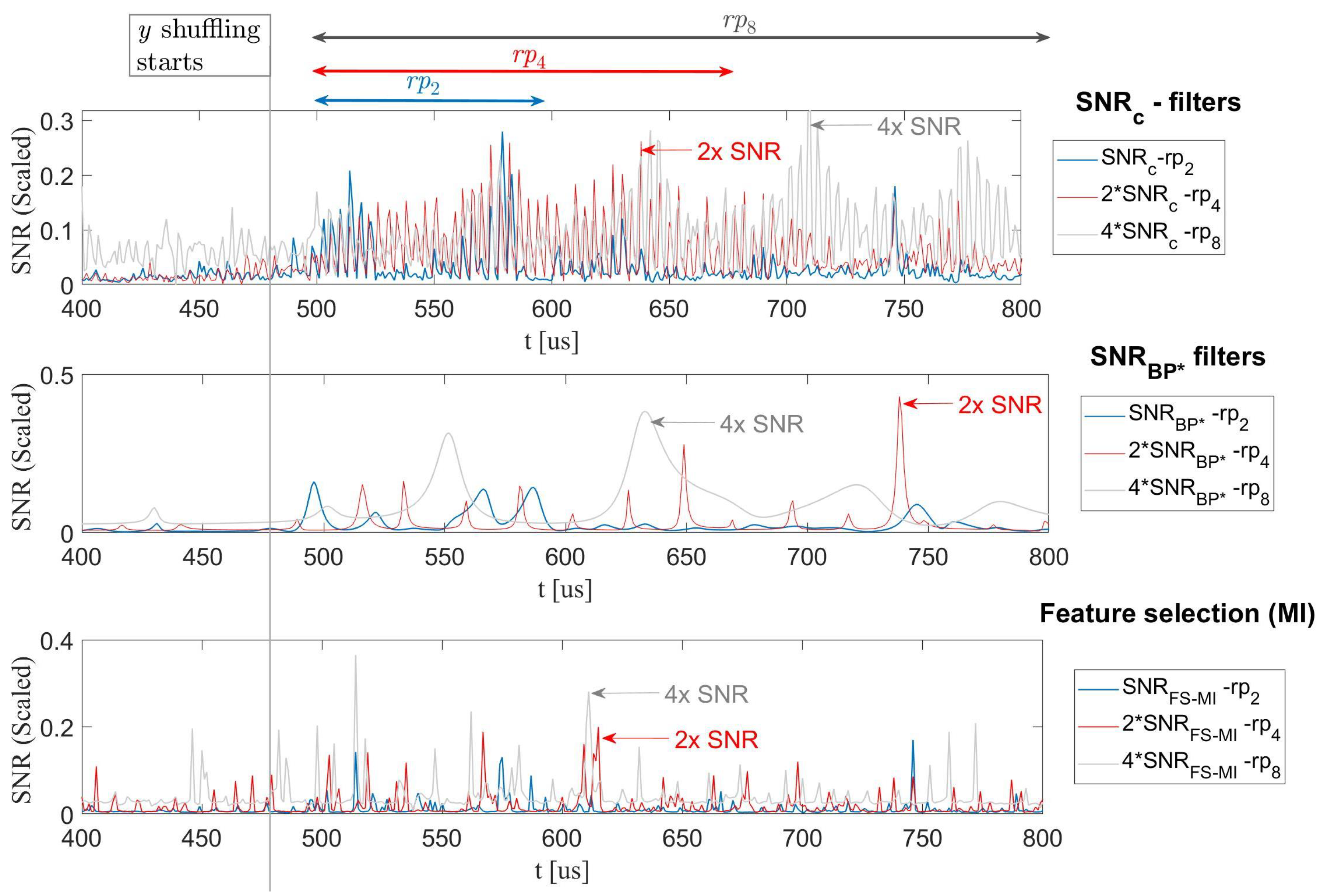
We next compared a software implementation of instruction shuffling to demonstrate the effect of different pre-processing techniques on different countermeasures and specifically on different shuffling implementations with different level of protection. Below, unshuffled refers to the basic unprotected software implementation, and shuffled to the case where i Sboxes’ computation order is permuted over (in sets of 16). We acknowledge that we cannot directly compare the following results to the hardware implementations due to the clear baseline difference in the SW case. However, the results still reveal important insights regarding pre-processing techniques. Thus, we only compare the different shuffling implementations to each other and to the unshuffled implementation. As can be seen in Figure 9, there was already a notable reduction in the univariate for all of the shuffling methods. Furthermore, as the number of shuffling instructions increased (time variance), the decreased. Clearly, as the number of shuffling instructions increased, the more peaks there were (i.e., the information is spread out). This observation led us to define different efficiency criterion, as shown in Equation (8).
Figure 10 shows the effect of different filters on the shuffled implementations. Note that in order to fit all the plots on the same graph, the of , were scaled. As noted on the graph, was scaled by a factor of 2, and by a factor of 4. This follows theory nicely where the levels decrease linearly with the number of shuffled instructions as the probability that a computation of the target Sbox will take place at the i-th round is uniform. Therefore, the reduction in is linear.
The top sub-figure in Figure 10 shows the levels of the filter applied to the shuffling implementations. It is clear that as the random permutation size increases, so does the length of time samples containing useful information (i.e., for from 500 to 600, for from 500 to 700, for from 500 to 800). We can further see that the number of peaks increases as the number of shuffling instructions increases (for two distinctive peaks, for four peaks, for at least four peaks, but with some aliasing due the leakage measurement impedance).
The middle sub-figure in Figure 10 shows the levels of the optimal BP-Filter applied on shuffling implementations. It is evident that this filter failed to deliver the same levels as the . Moreover, the optimal BPF smooths out the gains as compared to the filter. This was more pronounced in the of and (the smoothing action is compared to the filter). The smoothing effect actively reduced the time span in which distinct levels appeared; in turn, it reduced the overall informativeness (for our criterion in Equation (8)). The bottom plot in Figure 10 shows the levels of a univariate feature selection in the frequency domain applied on the shuffling implementations. This feature selection also creates a custom filter, but it also failed to keep up with the levels of the filter. We elaborate further on feature selection techniques in Section 4.1.2.
Figure 11 shows the rate of convergence of the different filters compared to the baseline . We used the metric of . The figures show the , denoted in abbreviated form by . This metric not only weighs the levels, but also the number of contributing time samples, compared to , which works on a single time point. Note that as discussed above, the data set was not large enough for full convergence, but still large enough to see considerable differences between the methods. To the right of each plot on the figure is a ‘zoom in’ view that visualizes the difference between the methods more clearly. In all cases, the filters were considerably better than the baseline , and as the permutation size increased, the amount of information extracted from the optimal BP-Filter decreased. In contrast, the results for the filters were more efficient. Another advantage of using the metric and showing the rather than is that the integral of the baseline over time remains the same, independently of the permutation size. It implies that the overall information leakage is preserved. Therefore, it is possible to compare the results of filters across .
For (top Sub-figure), filter yielded 1.878x compared to 1.798x for the Optimal BP-Filter, where 1x denotes no pre-processing. For , filter yielded 1.602x compared to 1.264x for the Optimal BP-Filter, and for , filter yielded 1.5161x compared to 1.332x for the Optimal BP-Filter. Thus, there was a considerable difference between and the optimal BPFs. Interestingly, the optimal filter gain was roughly 2x for the shuffling flavors (SW), but roughly 10x for the hardware implementations. This stems from the overall lower levels of noise present in software implementations; i.e., the potential to filter out noise is much lower in software, because the signal is already very large.
4.1.2. Multi Trace—A Cautionary Note on Feature-Selection Tools
It is interesting to compare popular filters from artificial intelligence (AI)/machine learning (ML) tools since they have become highly popular for pre-processing and SCA attacks (in a general context) [42,43,44,45]. For that purpose, we implemented various feature selection (FS) tools and processed them in the frequency domain over the FFT leakages to find the best shaped filter. The two main observations deriving from this analysis are that:
- As illustrated in the bottom plot in Figure 10, FS with complex statistical tools such as the Mutual-Information (MI) exhibit extremely poor results. This is clearly due to the fact that for information theoretic tools to function properly, the distribution of the leakage needs to be decently captured, which implies a large observation space; i.e., statistically, the full distribution is badly characterized and the filter is far from converging.
- More (statistically) simple FS tools were attempted, such as the Pearson-corr () to filter frequency coefficients.The experiments showed that it performed quite similarly to our SNR based criterion. However, consistently results were slightly poorer since the correlation was not scaled to the noise such as the SNR.
4.2. Single-Trace
As discussed above a spectogram provides considerable information relating to the type of filter required in the multi-trace context, but also in terms of the Z parameter and the spectral characteristics that change over time, which is important for OVSSA in the single-trace context. Figure 12 illustrates the spectogram of an exemplary trace taken from the unprotected CMOS rolled implementation (left), the dual-rail implementation (middle) and the shuffling SW implementation.
These spectograms can generate a good intuition as to whether a certain filter will work well or poorly. For instance, shuffling- demonstrates at least two dominant frequencies at any given time sample throughout the trace. The unprotected CMOS implementation exhibits only one dominant band, which is why, intuitively, BPFs will work well for unprotected CMOS, but not for shuffling. The dual-rail design demonstrates leakages at a smaller frequency than the CMOS design (since the precharege and evaluation phases generate a larger effective clock period). However, for all designs, the X-axis (time) shows that the spectrum characteristics change as discussed in Section 2.3.2.
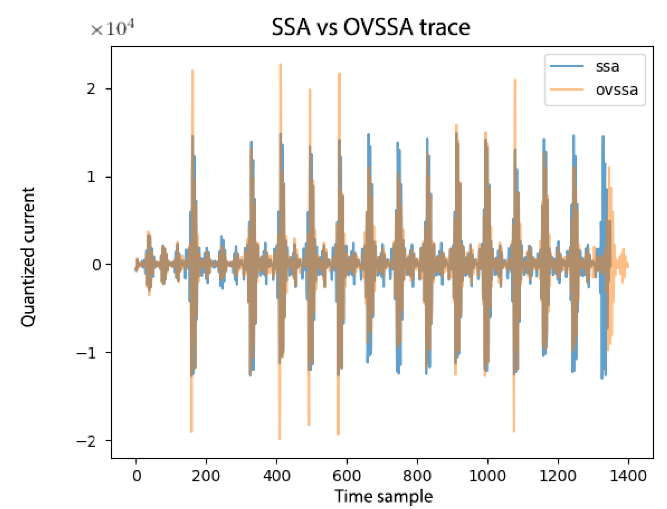
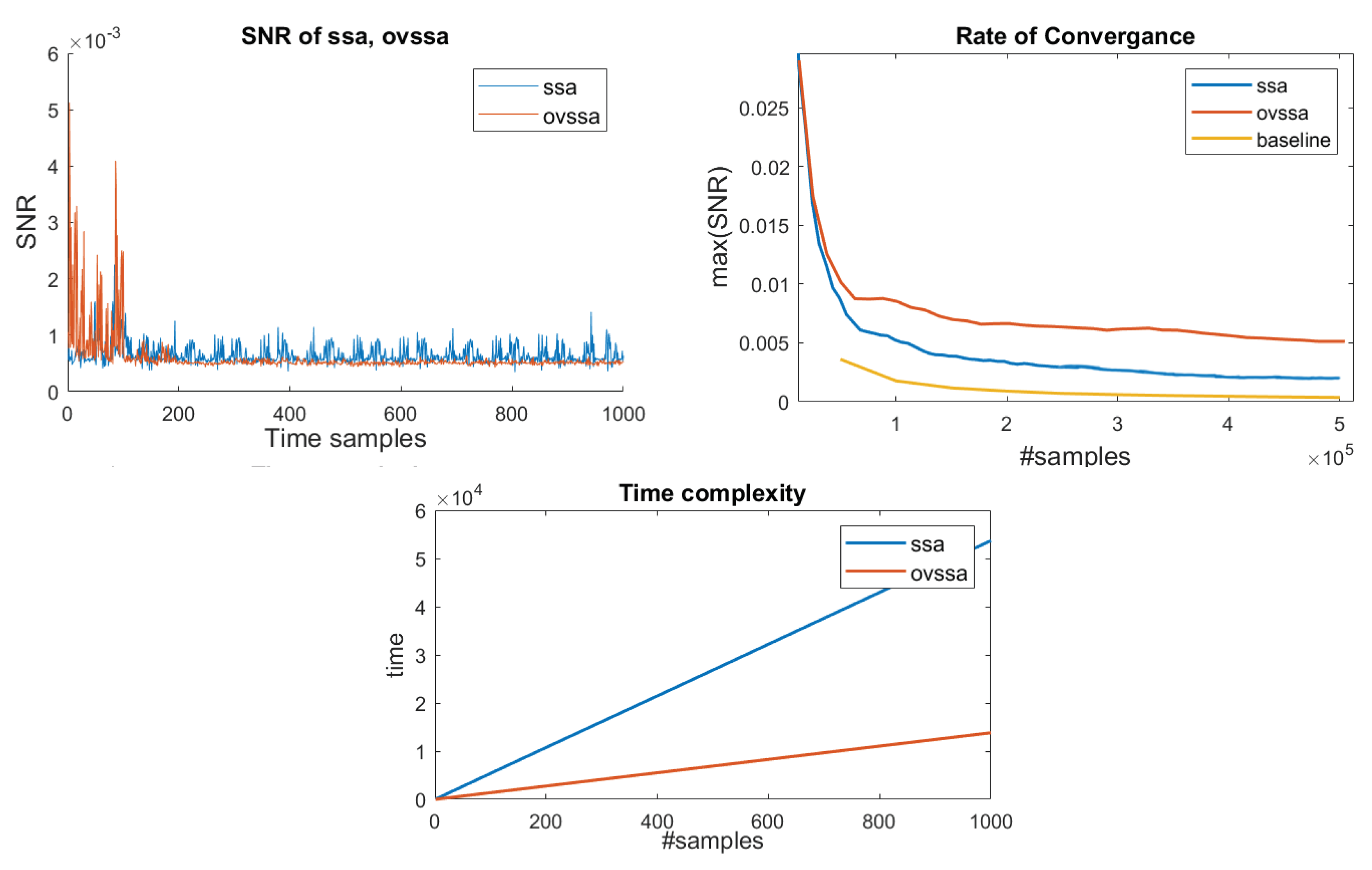
Overall, in this manuscript, we processed traces with SSA/OVSSA, where the goal was to capture enough cleaned traces to evaluate the of each technique as a comparison metric to evaluate performance. The processing took ∼5 months on a very powerful server with 50 machines where each multi-threaded over 20 processors. Each computation took about 30 s, compared to 10 s for OVSSA. Figure 13 shows two exemplary pre-processed traces; the resulting traces from the OVSSA and processing are significantly different as possible to see.
Figure 14 shows an exemplary following and OVSSA (with traces) in the top-left sub-plot. Clearly, the OVSSA generated larger amplitudes, but perhaps more importantly, the noise was significantly reduced. In this example, the was computed with y labeling following the first Sbox layer in an AES round, therefore peaks appear closer to the beginning of the trace. However, in later rounds we observed that the of the still exhibited small peaks where the y-classification was clearly wrong (diffusion); the OVSSA, however, cleans these regions nicely, as its indicates.
The top-right sub-plot in Figure 14 shows the convergence with the number of traces of the baseline {unprocessed traces, the SSA- and OVSSA- processed} traces. The plot shows that 0.2–0.3 traces are sufficient for convergence. The of all pre-processing techniques converged with similar data complexity. However, the maximum- achieved with was ∼2.5× as compared to unprocessed traces, while OVSSA achieved ∼5× improvement as compared to unprocessed traces.
The last important point as mentioned in Section 1 and Section 2.3.2, relates to the pre-processing time-complexity. The bottom sub-plot in Figure 14 shows the time complexity required to process the data set as a function of the data set size in samples. As both SSA/OVSSA worked on a single trace every time, both graphs are linear. Clearly, OVSSA had much lower time complexity, with a respective gain of ∼4× over (see next paragraph) due to the fact that OVSSA works on small segments of the trace, while works on the entire trace at once. All in all, OVSSA exhibited more efficiency than both in time complexity and information extraction ().
Concretely, the proposed technique provides ∼2× max. improvement for about the same number of leakage-traces (data-complexity), as compared to -based approach. However, the main improvement is in the pre-processing evaluation time. The time complexity of the based pre-processing technique depends on SVD, which is generally quadratic in time as a function of the number of leakage time samples, n. The OVSSA based pre-processing technique time complexity depends on SVDs over chunked leakage traces (fewer samples), with a parameter Z; i.e., chunks. That is, the time complexity improvement is generally , which was shown to be very significant in our experiments, although we failed to perfectly achieve the suggested gain of . This is due to software implementation variations, server computing power variations and neglected arithmetic. As discussed above, Z depends on the spectral characteristics of the leakage throughout time and for round-base cryptographic implementations the factor is expected to yield significant improvements as exemplified.
5. Conclusions
In this paper, we presented several advances in two SCA contexts. In the single-trace context, we improved upon existing SSA-based techniques by exploiting informative variations in spectral properties over time, stemming from the cryptographic implementation. By adapting overlapped-SSA and further optimizing over subsequent processing-related key parameters, we achieved a significant gain compared to SSA and no pre-processing, both in terms of (shorter) computation time and (higher) information gain, i.e., . In the multi-trace context, we proposed a profiling strategy for a BPF optimization based on a computationally attractive objective function, which was shown to be efficient for unprotected and weakly protected implementations (albeit with reduced effectiveness). In addition, we also proposed a differently optimized filter, exploiting frequency-domain -based coefficients thresholding, which is slightly more computationally demanding. The simulation results of our extensive empirical examination show the significant performance improvement over a set of implementations embedded with countermeasures, both in hardware and software platforms. In all the implementations/platforms we considered, our proposed shaped filter achieved the highest levels, while the BPF-based filters suffered from reduced effectiveness when applied to varying protection-level countermeasures embedded.
Author Contributions
Conceptualization, I.L. and D.S.; methodology, I.L., D.S. and A.W.; software, D.S.; validation, D.S. and I.L.; formal analysis, D.S., A.W. and I.L.; investigation, D.S.; data curation, I.L. and D.S.; writing–original draft preparation, I.L. and D.S.; writing–review and editing, D.S., A.W. and I.L.; visualization, D.S., A.W. and I.L.; supervision, I.L. All authors have read and agreed to the published version of the manuscript.
Funding
This research received no external funding.
Institutional Review Board Statement
Not applicable.
Informed Consent Statement
Not applicable.
Data Availability Statement
The data presented in this study are available in article.
Conflicts of Interest
The authors declare no conflict of interest.
References
- McKay, K.; Bassham, L.; Sönmez Turan, M.; Mouha, N. Report on Lightweight Cryptography; NIST Interagency/Internal Report (NISTIR); National Institute of Standards and Technology: Gaithersburg, MD, USA, 2017. [CrossRef]
- Standaert, F.X. Analyzing the Leakage-Resistance of some Round-2 Candidates of the NIST’s Lightweight Crypto Standardization Process. In Proceedings of the NIST Lightweight Cryptography Workshop, Gaithersburg, MD, USA, 4–6 November 2019. [Google Scholar]
- Camurati, G.; Poeplau, S.; Muench, M.; Hayes, T.; Francillon, A. Screaming channels: When electromagnetic side channels meet radio transceivers. In Proceedings of the 2018 ACM SIGSAC Conference on Computer and Communications Security, Toronto, ON, Canada, 15–19 October 2018; pp. 163–177. [Google Scholar]
- Benhani, E.; Bossuet, L.; Aubert, A. The Security of ARM TrustZone in a FPGA-based SoC. IEEE Trans. Comput. 2019, 68, 1238–1248. [Google Scholar] [CrossRef]
- Schellenberg, F.; Gnad, D.R.; Moradi, A.; Tahoori, M.B. An inside job: Remote power analysis attacks on FPGAs. In Proceedings of the Design, Automation & Test in Europe Conference & Exhibition (DATE), Dresden, Germany, 19–23 March 2018; pp. 1111–1116. [Google Scholar]
- Ramesh, C.; Patil, S.B.; Dhanuskodi, S.N.; Provelengios, G.; Pillement, S.; Holcomb, D.; Tessier, R. FPGA side channel attacks without physical access. In Proceedings of the 2018 IEEE 26th Annua l International Symposium on Field-Programmable Custom Computing Machines (FCCM), Boulder, CO, USA, 29 April–1 May 2018; pp. 45–52. [Google Scholar]
- Zhao, M.; Suh, G.E. FPGA-based remote power side-channel attacks. In Proceedings of the 2018 IEEE Symposium on Security and Privacy (SP), San Francisco, CA, USA, 21–23 May 2018; pp. 229–244. [Google Scholar]
- Provelengios, G.; Holcomb, D.; Tessier, R. Power wasting circuits for cloud FPGA attacks. In Proceedings of the 2020 30th International Conference on Field-Programmable Logic and Applications (FPL), Gothenburg, Sweden, 31 August–4 September 2020; pp. 231–235. [Google Scholar]
- Benhani, E.M.; Bossuet, L. Dvfs as a security failure of trustzone-enabled heterogeneous soc. In Proceedings of the 2018 25th IEEE International Conference on Electronics, Circuits and Systems (ICECS), Bordeaux, France, 9–12 December 2018; pp. 489–492. [Google Scholar]
- Ravi, P.; Poussier, R.; Bhasin, S.; Chattopadhyay, A. On Configurable SCA Countermeasures Against Single Trace Attacks for the NTT. In International Conference on Security, Privacy, and Applied Cryptography Engineering; Springer Nature Switzerland: Cham, Switzerland, 2020; pp. 123–146. [Google Scholar]
- Battistello, A.; Coron, J.S.; Prouff, E.; Zeitoun, R. Horizontal side-channel attacks and countermeasures on the ISW masking scheme. In Proceedings of the International Conference on Cryptographic Hardware and Embedded Systems, Santa Barbara, CA, USA, 25–28 September 2016; Lecture Notes in Computer Science (LNCS). Springer: Berlin/Heidelberg, Germany, 2016; pp. 23–39. [Google Scholar]
- Singh, A.; Kar, M.; Mathew, S.; Rajan, A.; De, V.; Mukhopadhyay, S. 25.3 A 128b AES engine with higher resistance to power and electromagnetic side-channel attacks enabled by a security-aware integrated all-digital low-dropout regulator. In Proceedings of the 2019 IEEE International Solid-State Circuits Conference-(ISSCC), San Francisco, CA, USA, 17–21 February 2019; pp. 404–406. [Google Scholar]
- Wong, C. Analysis of DPA and DEMA Attacks. Master’s Thesis, San Jose State University, San Jose, CA, USA, 2012. [Google Scholar] [CrossRef]
- Plos, T.; Hutter, M.; Feldhofer, M. On comparing side-channel preprocessing techniques for attacking RFID devices. In Proceedings of the International Workshop on Information Security Applications; Springer: Berlin/Heidelberg, Germany, 2009; pp. 163–177. [Google Scholar]
- Bu, A.; Dai, W.; Lu, M.; Cai, H.; Shan, W. Correlation-Based Electromagnetic Analysis Attack Using Haar Wavelet Reconstruction with Low-Pass Filtering on an FPGA Implementaion of AES. In Proceedings of the 2018 17th IEEE International Conference on Trust, Security and Privacy in Computing and Communications/12th IEEE International Conference on Big Data Science and Engineering (TrustCom/BigDataSE), New York, NY, USA, 1–3 August 2018; pp. 1897–1900. [Google Scholar]
- Oswald, D.; Paar, C. Breaking Mifare DESFire MF3ICD40: Power analysis and templates in the real world. In International Workshop on Cryptographic Hardware and Embedded Systems; Lecture Notes in Computer Science (LNCS); Springer: Berlin/Heidelberg, Germany, 2011; pp. 207–222. [Google Scholar]
- Kumar, R.; Liu, X.; Suresh, V.; Krishnamurthy, H.K.; Satpathy, S.; Anders, M.A.; Kaul, H.; Ravichandran, K.; De, V.; Mathew, S.K. A Time-/Frequency-Domain Side-Channel Attack Resistant AES-128 and RSA-4K Crypto-Processor in 14-nm CMOS. IEEE J. Solid-State Circuits 2021, 56, 1141–1151. [Google Scholar] [CrossRef]
- Park, A.; Han, D.G.; Ryoo, J. CPA performance comparison based on Wavelet Transform. In Proceedings of the 2012 IEEE International Carnahan Conference on Security Technology (ICCST), Newton, MA, USA, 15–18 October 2012; pp. 201–206. [Google Scholar]
- Vautard, R.; Yiou, P.; Ghil, M. Singular-spectrum analysis: A toolkit for short, noisy chaotic signals. Phys. D Nonlinear Phenom. 1992, 58, 95–126. [Google Scholar] [CrossRef]
- Del Pozo, S.M.; Standaert, F.X. Blind source separation from single measurements using singular spectrum analysis. In Proceedings of the International Workshop on Cryptographic Hardware and Embedded Systems; Lecture Notes in Computer Science (LNCS); Springer: Berlin/Heidelberg, Germany, 2015; Volume 9293, pp. 42–59. [Google Scholar]
- Leles, M.; Sansão, J.; Mozelli, L.; Guimarães, H. A new algorithm in singular spectrum analysis framework:The Overlap-SSA (ov-SSA). SoftwareX 2018, 8, 26–32. [Google Scholar] [CrossRef]
- Levi, I.; Bellizia, D.; Standaert, F.X. Beyond algorithmic noise or how to shuffle parallel implementations? Int. J. Circuit Theory Appl. 2020, 48, 674–695. [Google Scholar] [CrossRef]
- Cassiers, G.; Grégoire, B.; Levi, I.; Standaert, F.X. Hardware private circuits: From trivial composition to full verification. IEEE Trans. Comput. 2020, 70, 1677–1690. [Google Scholar] [CrossRef]
- Bilgin, B.; De Meyer, L.; Duval, S.; Levi, I.; Standaert, F.X. Low AND Depth and Efficient Inverses: A Guide on S-boxes for Low-latency Masking. IACR Trans. Symmetric Cryptol. 2020, 2020, 144–184. [Google Scholar] [CrossRef]
- Mangard, S. Hardware Countermeasures against DPA—A Statistical Analysis of Their Effectiveness. In Cryptographers’ Track at the RSA Conference; Lecture Notes in Computer Science; Springer: Berlin/Heidelberg, Germany, 2004; Volume 2964, pp. 222–235. [Google Scholar]
- Gierlichs, B.; Batina, L.; Tuyls, P.; Preneel, B. Mutual information analysis. In International Workshop on Cryptographic Hardware and Embedded Systems; Lecture Notes in Computer Science; Springer: Berlin/Heidelberg, Germany, 2008; pp. 426–442. [Google Scholar]
- Standaert, F.X.; Malkin, T.G.; Yung, M. A unified framework for the analysis of side-channel key recovery attacks. In Proceedings of the Annual International Conference on the Theory and Applications of Cryptographic Techniques, Cologne, Germany, 26–30 April 2009; Lecture Notes in Computer Science. Springer: Berlin/Heidelberg, Germany, 2009; pp. 443–461. [Google Scholar]
- Chari, S.; Rao, J.R.; Rohatgi, P. Template attacks. In International Workshop on Cryptographic Hardware and Embedded Systems; Lecture Notes in Computer Science; Springer: Berlin/Heidelberg, Germany, 2002; pp. 13–28. [Google Scholar]
- Gámiz-Fortis, S.; Pozo-Vázquez, D.; Esteban-Parra, M.; Castro-Díez, Y. Spectral characteristics and predictability of the NAO assessed through singular spectral analysis. J. Geophys. Res. Atmos. 2002, 107, ACL-11. [Google Scholar] [CrossRef]
- Du, K.; Zhao, Y.; Lei, J. The incorrect usage of singular spectral analysis and discrete wavelet transform in hybrid models to predict hydrological time series. J. Hydrol. 2017, 552, 44–51. [Google Scholar] [CrossRef]
- Afshar, K.; Bigdeli, N. Data analysis and short term load forecasting in Iran electricity market using singular spectral analysis (SSA). Energy 2011, 36, 2620–2627. [Google Scholar] [CrossRef]
- Hu, B.; Li, Q.; Smith, A. Noise reduction of hyperspectral data using singular spectral analysis. Int. J. Remote Sens. 2009, 30, 2277–2296. [Google Scholar] [CrossRef]
- Hattori, K.; Serita, A.; Yoshino, C.; Hayakawa, M.; Isezaki, N. Singular spectral analysis and principal component analysis for signal discrimination of ULF geomagnetic data associated with 2000 Izu Island Earthquake Swarm. Phys. Chem. Earth Parts A/B/C 2006, 31, 281–291. [Google Scholar] [CrossRef]
- Le Mouël, J.; Lopes, F.; Courtillot, V. Singular spectral analysis of the aa and Dst geomagnetic indices. J. Geophys. Res. Space Phys. 2019, 124, 6403–6417. [Google Scholar] [CrossRef]
- Hassani, H. Singular Spectrum Analysis: Methodology and Comparison; Cardiff University: Cardiff, UK; Central Bank of the Islamic Republic of Iran: Tehran, Iran, 2007. [Google Scholar]
- Gavish, M.; Donoho, D.L. The optimal hard threshold for singular values is 4/(30.5). IEEE Trans. Inf. Theory 2014, 60, 5040–5053. [Google Scholar] [CrossRef]
- Golyandina, N.; Nekrutkin, V.; Zhigljavsky, A.A. Analysis of Time Series Structure: SSA and Related Techniques; Chapman and Hall/CRC Press: Boca Raton, FL, USA, 2001. [Google Scholar]
- Nussbaumer, H.J. The fast Fourier transform. In Fast Fourier Transform and Convolution Algorithms; Springer: Berlin/Heidelberg, Germany, 1981; pp. 80–111. [Google Scholar]
- Montminy, D.P. Enhancing Electromagnetic Side-Channel Analysis in an Operational Environment. Ph.D Thesis, Air Force Institute of Technology, Wright Patterson Air Force Base, OH, USA, 2013. [Google Scholar]
- Belgarric, P.; Bhasin, S.; Bruneau, N.; Danger, J.L.; Debande, N.; Guilley, S.; Heuser, A.; Najm, Z.; Rioul, O. Time-frequency analysis for second-order attacks. In Proceedings of the 12th International Conference on Smart Card Research and Advanced Applications, Berlin, Germany, 27–29 November 2013; Springer: Berlin/Heidelberg, Germany, 2013; pp. 108–122. [Google Scholar]
- Tiu, C.C. A new Frequency-Based Side Channel Attack for Embedded Systems. Ph.D. Thesis, University of Waterloo, Waterloo, ON, Canada, 2005. [Google Scholar]
- Hospodar, G.; Gierlichs, B.; De Mulder, E.; Verbauwhede, I.; Vandewalle, J. Machine learning in side-channel analysis: A first study. J. Cryptogr. Eng. 2011, 1, 293. [Google Scholar] [CrossRef]
- Picek, S.; Heuser, A.; Jovic, A.; Ludwig, S.A.; Guilley, S.; Jakobovic, D.; Mentens, N. Side-channel analysis and machine learning: A practical perspective. In Proceedings of the 2017 International Joint Conference on Neural Networks (IJCNN), Anchorage, Alaska, USA, 14–19 May 2017; pp. 4095–4102. [Google Scholar]
- Picek, S.; Heuser, A.; Jovic, A.; Batina, L. A systematic evaluation of profiling through focused feature selection. IEEE Trans. Very Large Scale Integr. (VLSI) Syst. 2019, 27, 2802–2815. [Google Scholar] [CrossRef]
- Liu, J.; Zhang, S.; Luo, Y.; Cao, L. Machine Learning-Based Similarity Attacks for Chaos-based Cryptosystems. IEEE Trans. Emerg. Top. Comput. 2020. [Google Scholar] [CrossRef]
Figure 1.
Exemplary of AES leakage traces. (a) The eigenvalues in a decreasing order. (b) several components of the decomposition. (c) The original trace. Current measurements were performed with a 16-bit ADC.
Figure 1.
Exemplary of AES leakage traces. (a) The eigenvalues in a decreasing order. (b) several components of the decomposition. (c) The original trace. Current measurements were performed with a 16-bit ADC.

Figure 2.
A single leakage trace Spectogram of an unprotected standard (CMOS) rolled implementation of an AES.
Figure 2.
A single leakage trace Spectogram of an unprotected standard (CMOS) rolled implementation of an AES.

Figure 3.
DFT examples: (a) A cosine wave. (b) An unprotected CMOS AES encryption.

Figure 4.
Filter design and optimization: (a) Parameters of different (frequency) band-pass filters, and (b) exemplary general shaped filters.
Figure 4.
Filter design and optimization: (a) Parameters of different (frequency) band-pass filters, and (b) exemplary general shaped filters.

Figure 5.
Optimizing a band-pass filter: (a) SNR of filtered signal by SNR-FFT vs. filter thresholdfactor, (b) max SNR vs. frame width (bandwidth), and offset (slice number).
Figure 5.
Optimizing a band-pass filter: (a) SNR of filtered signal by SNR-FFT vs. filter thresholdfactor, (b) max SNR vs. frame width (bandwidth), and offset (slice number).

Figure 6.
Visual comparison between different filters (top) and SNR(t). (Bottom): (Left) unprotected CMOS, (Center) Dual-Rail, (Right) Shuffling .
Figure 6.
Visual comparison between different filters (top) and SNR(t). (Bottom): (Left) unprotected CMOS, (Center) Dual-Rail, (Right) Shuffling .

Figure 7.
SNR versus time of CMOS and dual-rail filtered leakages: (Top) , (Bottom) .

Figure 8.
Rate of convergence of different filters-different designs: Left: unprotected CMOS, Center: Dual-Rail, Right: Shuffling .
Figure 8.
Rate of convergence of different filters-different designs: Left: unprotected CMOS, Center: Dual-Rail, Right: Shuffling .

Figure 9.
SNR of different shuffling implementations.

Figure 10.
of different filters—shuffling: (Top) , (Center) , (Bottom) feature selection (FS).

Figure 11.
Rate of convergence—shuffling: (Top) , (Center) , (Bottom) .

Figure 12.
Spectogram of different designs: Left: unprotected CMOS, Center: Dual-Rail, Right: Shuffling .
Figure 12.
Spectogram of different designs: Left: unprotected CMOS, Center: Dual-Rail, Right: Shuffling .

Figure 13.
Post-SSA vs. post-OVSSA leakage trace. Current measurements were performed with a 16-bit ADC.
Figure 13.
Post-SSA vs. post-OVSSA leakage trace. Current measurements were performed with a 16-bit ADC.

Figure 14.
SSA vs. OVSSA: Top-Left: (t) post-SSA and post-OVSSA, Top-Right: Rate of convergence of max(), Bottom: Preprocessing time complexity versus the number of time samples in a trace.
Figure 14.
SSA vs. OVSSA: Top-Left: (t) post-SSA and post-OVSSA, Top-Right: Rate of convergence of max(), Bottom: Preprocessing time complexity versus the number of time samples in a trace.


Table 1.
Summary of the main results: Upper (resp. lower) half of the table list comparison values of the single- (resp. multiple-) trace context.
Table 1.
Summary of the main results: Upper (resp. lower) half of the table list comparison values of the single- (resp. multiple-) trace context.
| Technique | Context | x(SNR) | x(Time) | x(Data) | Counter. * |
|---|---|---|---|---|---|
| No filtering (baseline) | Single | 1 | 1 | 1 | CMOS-none |
| Adapting SSA [19,20] | Single | 2.5 | 1 | 1 | CMOS-none |
| Proposed (adapting [21]) | Single | 5 | 1 | CMOS-none | |
| No filtering (baseline) | Multi | 1 | 1 | 1 | Dual Rail |
| Optimized BPF (proposed) | Multi | 6.74 | 1 | 2.5 | Dual Rail |
| Shaped filter (proposed) | Multi | 10.75 | 1 | 2.5 | Dual Rail |
Various implementations with countermeasures were evaluated. Here, we exemplify through our implementation yielding the largest improvement. No filtering serves as a baseline for comparison.
Table 2.
Summary table of all designs evaluated in this paper.
| Design Name | #Traces | Base-Line | Protection Mechanism | Platform |
|---|---|---|---|---|
| CMOS | None | 65 nm ASIC (HW) | ||
| Dual-Rail | WDDL implementation | 65 nm ASIC (HW) | ||
| Amp.-Rnd. | Amplitude rand. technique | 65 nm ASIC (HW) | ||
| Shuffling | 6144 | Rand. instr. perm. | 40 nm Atmel 8-bit C (SW) |
Table 3.
Legend of names and abbreviations used in the manuscript and Section 4.
Table 3.
Legend of names and abbreviations used in the manuscript and Section 4.
| Context | Method Name | Description |
|---|---|---|
| Single | Singular Spectrum Analysis | |
| Single | OVSSA | Overlapping and segmented |
| Multi | BP-filter | BPF, optimally fitted for each design |
| Multi | Filter based on threshold of the freq. coeffs. (Shaped) | |
| Multi | MI-FS | Mutual Information based Feature Selection of freq. coeffs. |
Publisher’s Note: MDPI stays neutral with regard to jurisdictional claims in published maps and institutional affiliations. |
© 2021 by the authors. Licensee MDPI, Basel, Switzerland. This article is an open access article distributed under the terms and conditions of the Creative Commons Attribution (CC BY) license (https://creativecommons.org/licenses/by/4.0/).
Share and Cite
MDPI and ACS Style
Salomon, D.; Weiss, A.; Levi, I. Improved Filtering Techniques for Single- and Multi-Trace Side-Channel Analysis. Cryptography 2021, 5, 24. https://0-doi-org.brum.beds.ac.uk/10.3390/cryptography5030024
AMA Style
Salomon D, Weiss A, Levi I. Improved Filtering Techniques for Single- and Multi-Trace Side-Channel Analysis. Cryptography. 2021; 5(3):24. https://0-doi-org.brum.beds.ac.uk/10.3390/cryptography5030024
Chicago/Turabian StyleSalomon, Dor, Amir Weiss, and Itamar Levi. 2021. "Improved Filtering Techniques for Single- and Multi-Trace Side-Channel Analysis" Cryptography 5, no. 3: 24. https://0-doi-org.brum.beds.ac.uk/10.3390/cryptography5030024