Seasonal Variation of Captive Meagre Acoustic Signalling: A Manual and Automatic Recognition Approach

Abstract

Many species rely on acoustic communication to fulfil several functions such as advertisement and mediation of social interactions (e.g., agonistic, mating). Therefore, fish calls can be an important source of information, e.g., to recognize reproductive periods or to assess fish welfare, and should be considered a potential non-intrusive tool in aquaculture management. Assessing fish acoustic activity, however, often requires long sound recordings. To analyse these long recordings automatic methods are invaluable tools to detect and extract the relevant biological information. Here we present a study to characterize meagre (Argyrosomus regius) acoustic activity during social contexts in captivity using an automatic pattern-recognition methodology based on the Hidden Markov Model. Calls produced by meagre during the breading season showed a richer repertoire than previously reported. Besides the dense choruses composed by grunts already known for this species, meagre emitted successive series of isolated pulses, audible as ‘knocks’. Grunts with a variable number of pulses were also registered. The overall acoustic activity was concurrent with the number of spawning events. A diel call rhythms exhibit peak of calling activity from 15:00 to midnight. In addition, grunt acoustic parameters varied significantly along the reproduction season. These results open the possibility to use the meagre vocal activity to predict breeding and approaching spawning periods in aquaculture management.

1. Introduction

Many species of fish are soniferous, producing sound in different activities, such as feeding, territorial behaviour and during reproductive activities [1,2]. In some species, the vocalizations associated with the latter are often produced in choruses [3]. These sounds can provide information about the caller to the recipient as they are associated with differences between species, between individual callers of the same species and between call types emitted by the same individual under different behavioural contexts [4]. The species-specificity of fish calls and intra-specific variation can also be important for researchers as it may enable the recognition of the vocal species and, for example, whether the animal is breeding or not.

While traditional survey methods are expensive, time consuming and dependent on weather conditions and human effort, passive acoustic monitoring (PAM) coupled with automatic recognition methods is emerging as a cost-effective non-intrusive method to monitor vocal animals in the wild as well as habitat health and biodiversity at temporal and geographical scales [5,6,7,8,9,10]. Consequently, PAM can be an efficient method to detect vocal fish and identify the onset, duration, and periodicity of reproductive activities and possibly changes in fish abundance [11,12]. This information is crucial for the management of exploited species (i.e., seasonal fishery closures designed to protect spawning fish) and conservation of essential fish habitat. However, to develop automatic recognition methods the acoustic repertoire of the target species needs to be characterised [8,13,14,15,16,17].

Sciaenids, known as croakers and drums, are soniferous fishes that produce breeding sounds (drums or grunts) through the contraction of a pair of sonic muscles typically present in males, and occasionally in both sexes, that cause the swimbladder to vibrate [18]. Sound production during the reproductive season has been reported in a number of sciaenid species, such as the weakfish, Cynoscion regalis [19], meagre, Argyrosomus regius [20], Japanese croaker, Argyrosomus japonicus [13] and red drum, Sciaenops ocellatus [21]. The profusion of advertisement calls produced by the representatives of this family during the reproductive season suggests that sound production might play an important role in their reproduction, and some studies have shown such association [22,23,24,25].

The meagre (Argyrosomus regius, Asso 1801) is one of the world’s largest marine teleosts and has a high commercial value for recreational and small-scale commercial fisheries and aquaculture [26]. Advertisement calls produced during spawning aggregations have been characterised for A. regius by Lagardère and Mariani [20]. According to these authors, meagre calls were produced in dense choruses in which two sound types could be identified: Long and short grunts. However, there is still a lack of information on the daily and seasonal variation of sound production by adult meagre. In addition, it is still not known how sound features vary throughout the spawning season.

Some methods have been reported to study extensive bioacoustic recordings. The most common are supervised detection methods that can use, for example, energy thresholds or a matched filter to uncover the sounds. In recent decades, the interest of automatic speech recognition allowed the development of methods for recognition of sound patterns that have become increasingly faster, accurate and robust. Unsupervised methods using machine learning, such as Gaussian mixture models (GMMs) [27], artificial neural networks (ANN) [28,29] and hidden Markov models (HMMs) [30,31,32,33,34], have been reported to successfully recognize and classify human and other animals’ vocalizations. In particular, HMMs can be used to statistically model both temporal and spectral variations of acoustic patterns through robust algorithms that extract the relevant information and ultimately classify the acoustic patterns.

Table 1. Examples of marine animal sound recognition systems.

Class		Objective	System	Feature	Reference
Fish	Meagre	C	HMM	MFCC a	Present study
	Lusitanian toadfish	I,C	HMM	MFCC, LPC, a	[15]
	Plainfin midshipman	C	SVM	MRAF	[36]
	4 grouper species	S	KNN, SVM, Sparse	(W)MFCC, (W)MRAF	[37]
	4 sciaenid species	S	f	SPL	[38]
	On-line fishes sound database	S	SVM	MFCC, LFCC, SE, SL	[39]
	Unknown fishes	Fish sound detection	PC-NMF, GMM		[40]
			SVM, KNN, NLR	MFCC,a	[41]
		C	RF, SVM	MFCC,a	[42]
Mammals	Cetaceans	S	ANN	SCF	[43]
		C	ANN	b	[44]
		C	ANN	c	[45]
		C	HMM	LPCC, MFCC	[46]
		S	g		[47]
		C,S	GMM	a, i	[48]
		S	h	a	[49]
		C	HMM		[9]
		S	g		[50]
		S	ANN	e	[51]
	Sea lions	I	ANN	d	[52]

ANN, artificial neural network; C, call type; GMM, Gaussian mixture model; HMM, hidden Markov model; I, individual; KNN, K-nearest neighbours; LPCC, linear prediction cepstral coefficients; MFCC, Mel-frequency cepstral coefficients; MRAF, multiresolution acoustic features; S, species; SCF, spectrogram correlator filter; Sparse, Sparse classification; SPL, sound pressure level; SVM, support vector machine; ^a vector composed of several sound coefficients/parameters; ^b each vocalization was characterized by its simultaneous modulations in duty cycle and peak frequency; ^c features were selected using a local discriminant basis; ^d average logarithmic spectrum on the backpropagation network input layer; ^e a wavelet coefficient matrix, plus a frequency features and time feature; ^f SPL feature-based signal detector using a correlation coefficient to measure the matching with the training selected data; ^g a contour-based classifier that applies a number of noise-cancellation techniques to a spectrogram and then searches for connected regions of data which rise above a pre-determined threshold; ^h a generalized tonal sound detector for extracting representative frequencies of delphinid whistles; ⁱ cepstral coefficient features with first and second derivatives, unpredictability measure feature and MUSIC algorithm feature.

refers to examples of automatic recognition systems for calls of different marine animals.

In this study, we characterised the calls produced by adult meagre and developed an automatic recognition system to analyse the round-the-clock (24 h/day) recordings made during 7 months in aquaculture facilities. Acoustic studies carried out in captive environments can provide valuable insights to the vocal behaviour of wild populations (e.g., [22,35]). The specific objectives were to (i) create a library of calls; (ii) create an automated recognition system to detect and classify meagre calls and apply this to the acoustic files recorded between January and July; (iii) compare results between the automatic and the manual approach; and (iv) investigate diel and seasonal patterns of calling activity, namely in relation to the breeding season.

2. Results

Captive meagre produced low-frequency pulsed calls with most energy below 1 kHz (see Materials and Methods ). The number of pulses in a sound varied from 1 to 160 (mean ± SD, 46.1 ± 33.0), sound duration varied from 38 to 2480 ms (799.6 ± 587.5), pulse period from 11.8 to 24 ms (17.4 ± 2.0) and peak frequency from 100 to 627 Hz (226.9 ± 147.5) (N = 222 calls). For this study calls were manually classified into 6 different categories based on the number of pulses to accommodate previous descriptions [20]: Long grunts (>30 pulses), intermediate grunts (7–29 pulses), short grunts (4–6 pulses), and 1 pulse, 2 pulses and 3 pulses. The shortest sound categories (1 pulse, 2 pulses and 3 pulses) were joined into one class for the automatic recognition system (see material and methods for more details). Many grunts recorded in the tanks presented irregular pulse periods and amplitude modulation in the first pulses (cf. Materials and Methods). Often grunts began with smaller pulse periods.

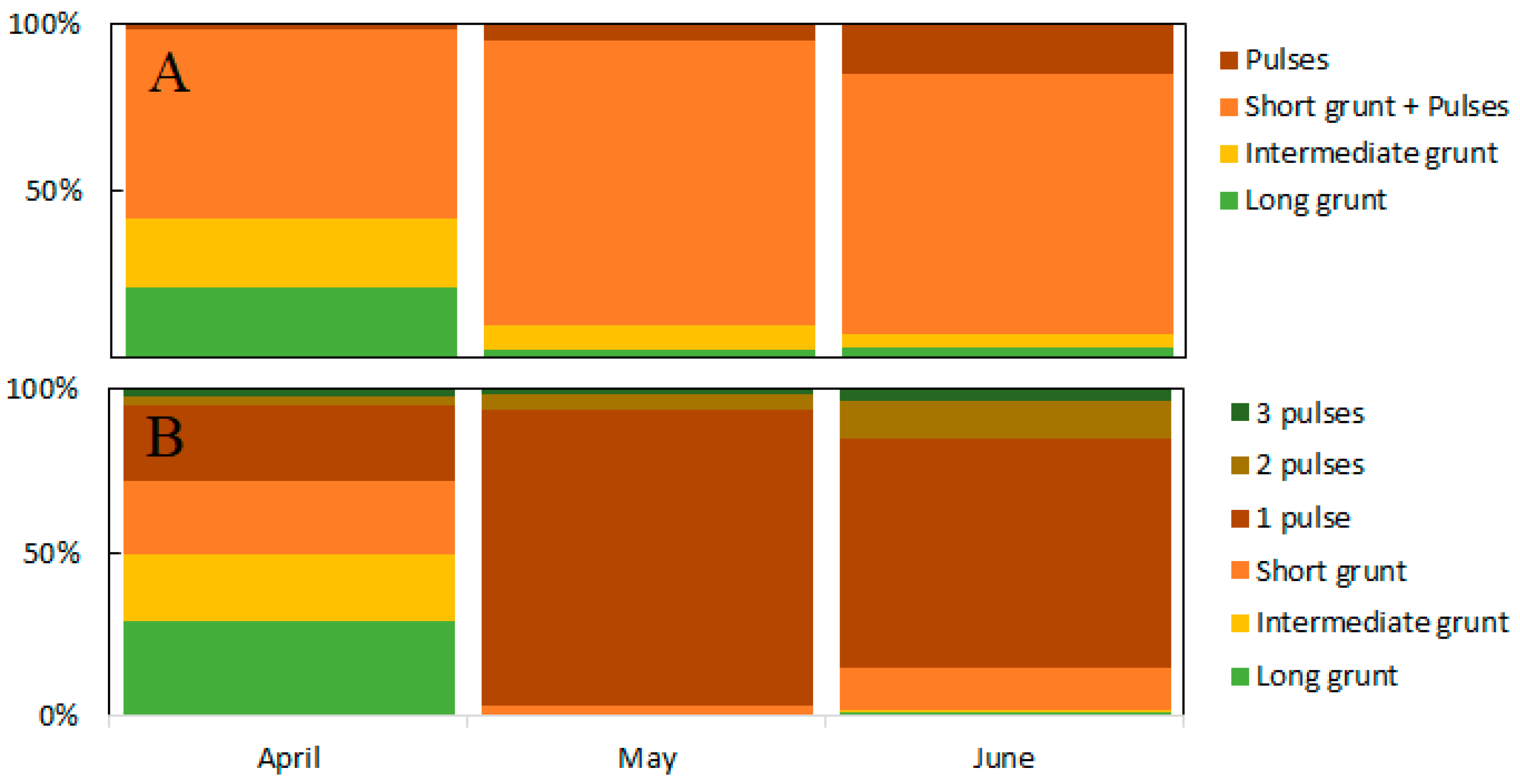
2.1. Validation of the Automatic Recognition System: Automatic Versus Manual Detection

The 20–2000 Hz bandwidth allowed the best recognition rate of meagre calls by the defined categories on the recognition system. A mean identification rate of 43.3% (and an accuracy of 2.2%) was obtained for the overall system using as test the recordings from 6 days (March 28th; April 18th and 28th, May 18th and 28th, and June 18th). But if joint categories were considered: ‘long grunts + intermediate grunts’, and ‘short grunts + pulses’, the overall mean rose to 78.8% (with an accuracy of 76.6%) due to the type of substitution errors observed. For example, most of the long grunts with less than 45 pulses were classified as intermediate grunts. In addition, some mistakes were observed on the limit of intermediate and short grunts (e.g., short grunts with 6 pulses were classified as intermediate grunts). The majority 1–3 pulses calls were misclassified as short grunts (Figure 1), as such, on the seasonal and diel analyses, the short grunt category will be referred to as the ‘short grunt + pulses’ category. Some intermediate grunts were also segmented into 2 short grunts (1 substitution error and 1 false positive). Most false negatives reported on pulses were observed in choruses with sequences of pulses due to misclassification of several pulses as one short grunt (e.g., 4 sequential pulses classified as a short grunt, origin one substitution error and 3 false negatives). Most calls with a signal-to-noise ratio under circa 4 dB were correctly ignored by the system, avoiding calls produced by fish housed in adjacent tanks.

Table 2. Confusion matrix from the hidden Markov model classification computed on the Mel-frequency cepstral (MFC) with energy, delta and acceleration coefficients with a frequency bandwidth of 20 Hz to 2000 Hz. The model was trained with 151 calls manually detected and classified, and tested with 18 h of recordings from 6 days (March 28th; April 18th and 28th, May 18th and 28th, and June 18th). Correct classifications are highlighted in bold in the matrix diagonal.

	Predicted Group Membership
Sound type	LG	IG	SG	Pulses	False negative	Correct identification rate (%)
Long grunt (LG)	39	108	0	0	1	26.4	95.0
Intermediate grunt (IG)	1	345	20	0	4	93.2
Short grunt (SG)	0	20	1485	12	30	96.0	76.8
Pulses	0	0	1568	175	915	6.6
False positive	0	3	121	7
Overall mean						43.3 %	78.8 %

represents the confusion matrix.

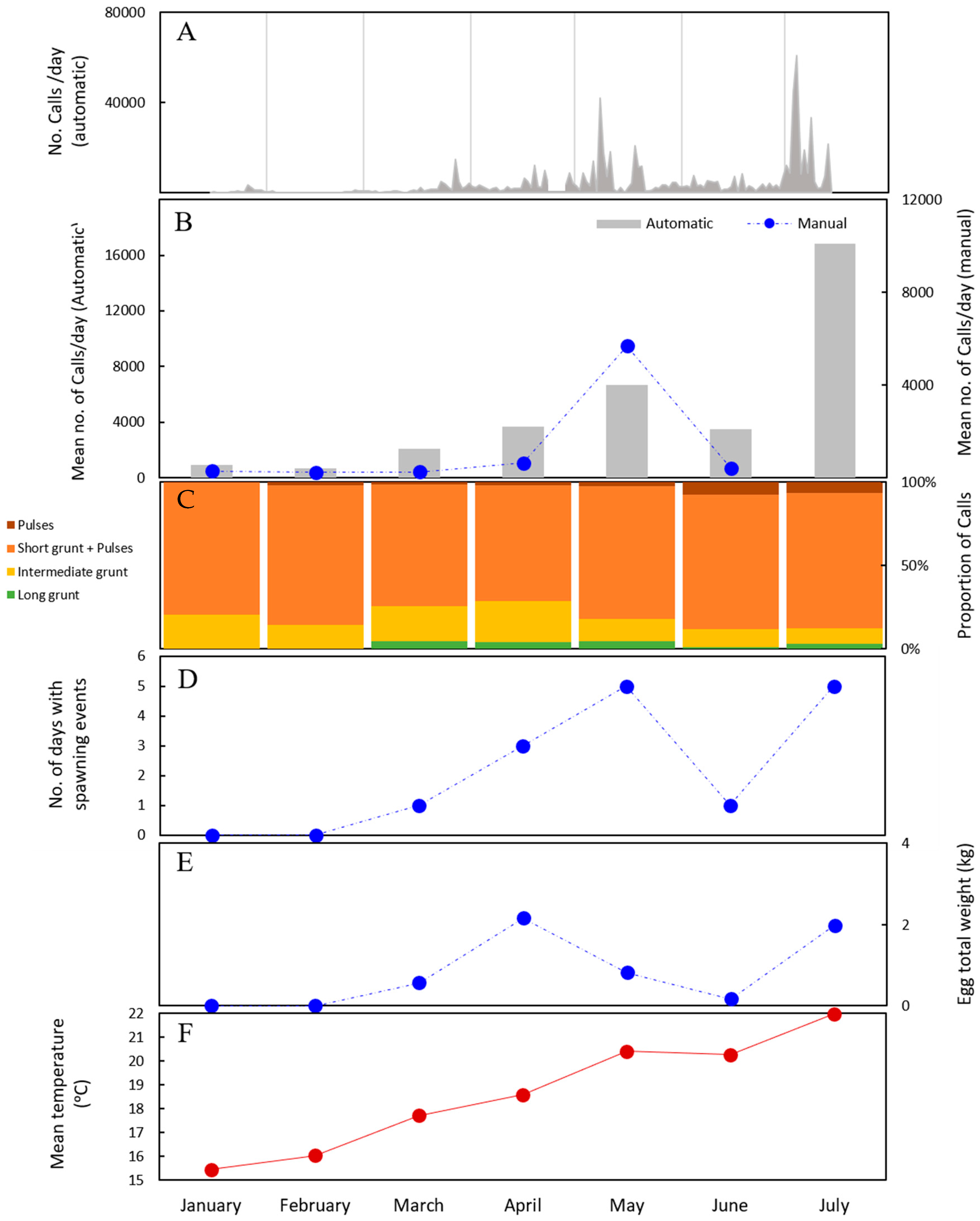
2.2. Seasonal Changes in Calling Rate

From January to May, the number of calls produced markedly increased (Figure 2A,B). The lowest number of detected calls occurred from January to March. In January, February, March, April and May, in the days/hours sampled, we manually counted a mean of 134, 115, 123, 317 and 2839 calls per day, respectively. In June, the number of calls detected manually decreased to a mean of 210 calls (Figure 2B). Similarly, the automatic recognition system, using all available recordings, showed an analogous call rate trend throughout the spawning season. In July, the number of calls detected by the recognition system increased concurrently to the number of spawning events. This is consistent with the occurrence of peaks in acoustic activity during the breeding season (Figure 2A). Note that, even ignoring most calls with a signal-to-noise ratio under circa 4 dB the recognition system still detected some calls produced by fish in adjacent tanks.

We assessed the variation of the different call categories throughout the breeding season using the automatic recognition system. The mean daily percentage of calls with 13 pulses, which were not discriminated by this system, increased from January (0.3%) to July (7.5%) (Figure 2). Detailed inspection, using manual annotation, of the recordings obtained in the period April to June revealed that calls composed of 2 and 3 pulses co-occurred with one pulse sequences. The calls with 2 and 3 pulses were, however, in a much lower proportion (Figure 1). The increase in the occurrence of these calls was more evident than depicted in Figure 2C, since many of the calls classified as ‘short grunt + pulses’ by the automatic recognition system were indeed calls with 1–3 pulses (see Figure 1). March, April and May were the months with the higher percentage of long grunts (4.7, 4.2 and 4.8% of all calls, respectively), and May showed the highest daily mean number of long grunts (562). The proportion of intermediate grunts increased from February (14.0%) to April (24.4%), and then decreased until July (10.8%). The highest percentage of short grunts + pulses occurred in February (83.4%), but the highest number of short grunts + pulses was observed in May (a mean of 9366 calls per day).

Notice that the mean water temperatures, computed per month, steadily increased from January to July (18 °C to 22 °C; Figure 2F).

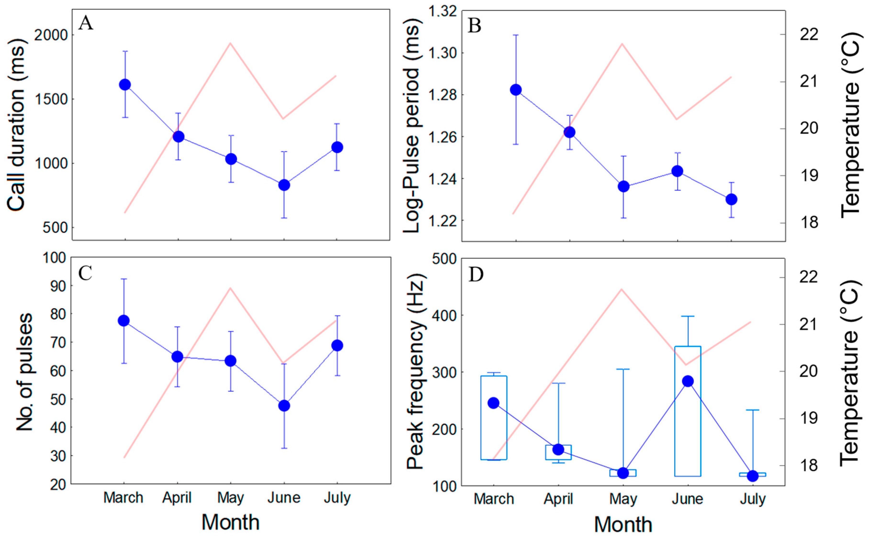
2.3. Seasonal Changes in Sound Features

Acoustic parameters of long grunts varied significantly among months. Sound duration (One-Way ANOVA; F_4,75 = 5.22, p < 0.001) and number of pulses (One-Way ANOVA; F_4,75 = 2.20, p = 0.08) decreased from March to June, and increased in July (Figure 3A,C;

Table 3. Call duration, number of pulses, pulse period and peak frequency of long grunts produced by captive Argyrosomus regius from March to July.

Sound Parameters		March	April	May	June	July
Call duration (ms)	Mean ± SD	1613 ± 376	1208 ± 405	1034 ± 436	831 ± 227	1127 ± 468
	Range	1112–2230	524–1835	449–2176	517–1348	646–2480
No. of pulses	Mean ± SD	77 ± 18	65 ± 21	63 ± 26	48 ± 13	69 ± 30
	Range	54–109	30–95	30–130	30–78	39–160
Pulse period (ms)	Mean ± SD	21 ± 1	19 ± 1	16 ± 1	18 ± 0.3	17 ± 0.4
	Range	21–23	18–20	15–17	17–18	15–17
Peak frequency (Hz)	Mean ± SD	230 ± 62	200 ± 100	151 ± 64	258 ± 104	124 ± 26
	Range	146–299	141–563	117–305	117–398	117–234

). Pulse period (One-Way ANCOVA; F_4,75 = 8.24, p < 0.001) decreased from March to May, increased in June and decreased again in July. The covariate temperature only had a significant effect in the pulse period; the pulse period decreased with water temperature (F_1,75 = 10.56, p = 0.002) (Figure 3B; Table 3). On the sampled days, water temperatures increased rapidly from March to May (18 to 22 °C), decreased in June (from 22 to 20 °C) and increased again in July (21 °C). Peak frequency showed a similar trend to the pulse period (Kruskal-Wallis test, H = 36.64, p < 0.001) (Figure 3D; Table 3).

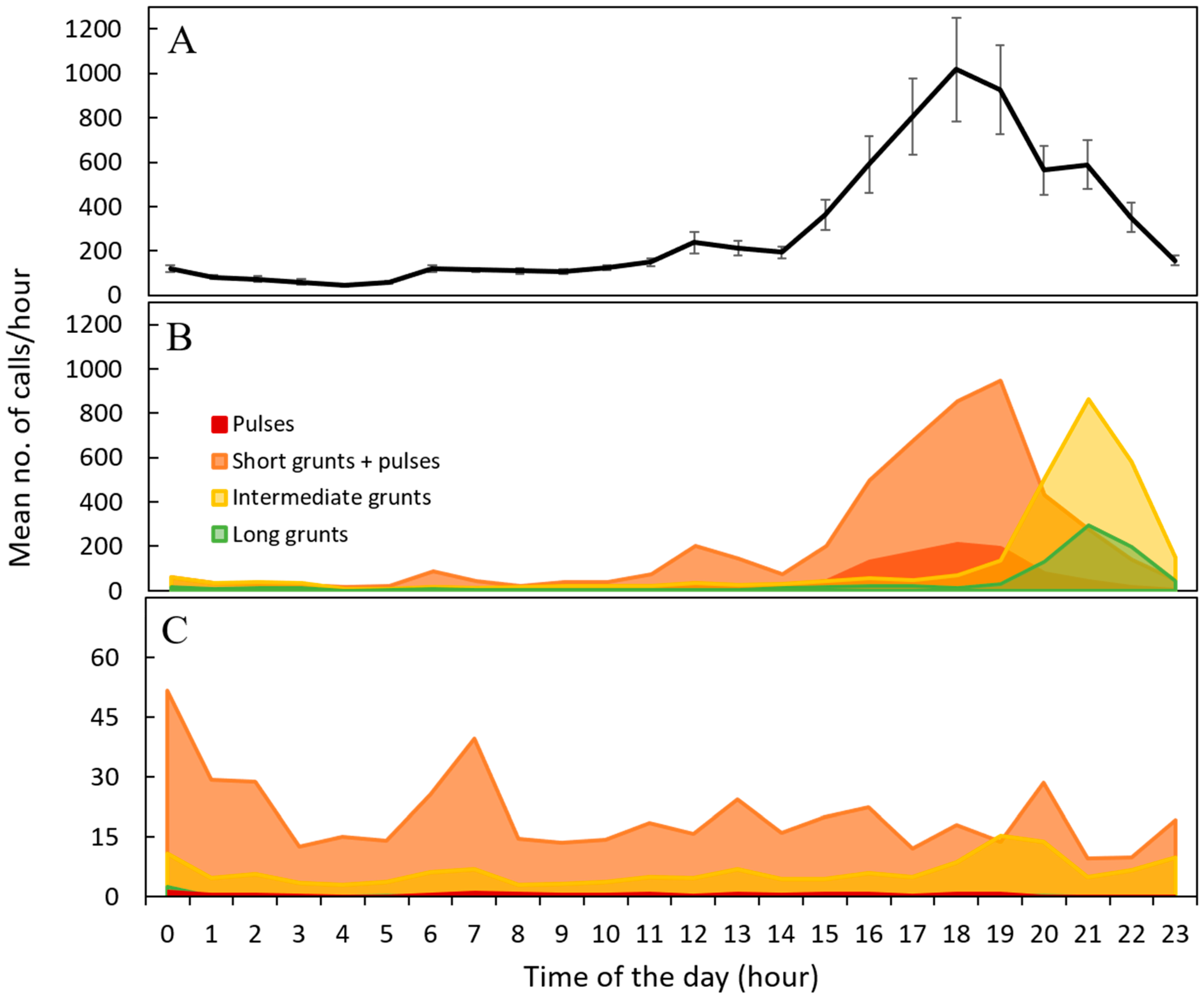
2.4. Diel Changes in Calling Rate

Mean call rates varied with time of day, with call rates peaking near sunset period and dropping off before midnight (Figure 4A). Interestingly, preliminary visualization of calling activity suggested at least two types of rhythms, depending on the overall daily number of calls. Thus, days were ranked by the number of calls counted per day and classified in percentiles. On the days with lower acoustic activity (25th percentile) and no chorusing behaviour, calls were more evenly produced throughout the 24 h cycle (Figure 4C). When the acoustic activity increased (75th percentile), the call rates peaking between 15:00 and midnight were clearly pronounced, reaching a mean calling rate of 1480 calls/hour at 21:00 (Figure 4B). Furthermore, the longer sound categories seem to appear later in the night (Figure 4B). Note that the distinction of sound categories depicted in Figure 3 was obtained by the automatic recognition system, and, as mentioned above, it recognised a high proportion of pulse calls as short grunts.

3. Discussion

Our study registered calls from captive meagre during 7 months and shows that A. regius has a greater variety of vocalizations than previously thought. According to Lagardère and Mariani [20], this species produces two sound types, short grunts (4–6 pulses) and long grunts (30–112 pulses). In this study, however, 6 putative categories (i.e., 1, 2 and 3 pulses, short, intermediate and long grunts) were observed, all of which appeared to be associated with the breeding season. The different sound categories mainly differed in the number of pulses (and hence duration) as is common for the majority of sciaenids (e.g., number of pulses and call duration [19,53,54]). The distinction of meagre calls in validated sound types still warrants a more detailed analysis of its repertoire [55] but a richer variability of the meagre’s acoustic repertoire is evident. Noticeably, calls made with 1–3 pulses, observed in long sequences, are clearly heard as knocking sounds in contrast with calls with more pulses that are heard as drumming sounds. Long grunts produced in captivity were similar to the ones found in the Gironde estuary [20] but in our study these calls exhibited a higher number of pulses, with a maximum of 160 pulses, in contrast with the 112 pulses described for the Gironde estuary. Interestingly, many grunts started with a faster pulse rate and amplitude modulation. This might be caused by changes in the sonic muscles’ contraction period and strength, or in the bilateral coordination of the sonic muscles that might alternate in the beginning and later become synchronized. This is likely dependent on the central pattern generator.

We used the manually-detected calls to create a library to train the HMMs in the automatic recognition system. We considered the same categories indicated above, except that the 1, 2 and 3 pulse calls were joined into a single category. Our automatic recognition system had difficulties with correctly discriminating some of the categories of meagre calls. For instance, some short grunts with 5 and 6 pulses, and the majority of long grunts with less than 45 pulses were classified as intermediate grunts. Moreover, many 1–3 pulse calls were classified as short grunts. The meagre system successfully detected all call types but the observed substitution errors probably occurred because we tried to classify a continuum in sound pulse numbers into an artificial discrete set of categories that may not constitute distinct call types. The lowest identification rate was 6.6% with the pulses that were in most part incorporated in the short grunt category. Notice, however, that almost all calls classified as pulses were pulses. In addition, the noise in the aquaculture facility caused a reduction in the signal-to-noise ratio of calls, leading to some misclassified calls. When the four call categories in Table 2 were grouped in only two categories, i.e., ‘long + intermediate grunts’ and ‘short grunt + pulses’, the automatic recognition system showed a higher and usable identification rate. The identification rates obtained for these joint categories are similar to the one obtained with the system developed for the boatwhistle calls of Lusitanian toadfish, which had an identification rate higher than 90%, but which failed to correctly recognize other call types (i.e., croaks and grunts) [15].

The application of automatic classification methods to fish calls is still scarce (Table 1). The work of Malfante et al. [42], using support vector machine algorithms (SVM), showed high accuracy with continuous recordings (average accuracy reaches 93.4%). Notice that, in contrast to meagre calls that exhibit a constant frequency spectrum, those authors classified call types with very distinct temporal and spectral features, which should make a correct automatic classification easier. Moreover, the same authors analysed consecutive fixed segments of 0.5 s not taking into account adjacent time windows, thus considering a sound encompassing more than one segment as more than one hit. This is an important limitation of the recognition system, e.g., for call counting operations or assessing call boundaries. Instead, HMM-based systems statistically model both temporal and spectral sound variations along a recording that permits recognition of the start and end time of each call, thus allowing call-counting operations. Monczak et al. [38], working on an estuarine soundscape in the May River (South Carolina, USA), distinguished the calls from four different sciaenid species with a good identification rate (higher than 61%), but did not discriminate call types within each species. Note that their validation method used a qualitative manual approach. Contrary to the work of Monczak et al. [38], we were not faced with the challenge of calling overlaps. Calling overlaps, however, occur in choruses by wild meagre aggregations, and these impose a challenge for acoustic monitoring. Analysing choruses with a high rate of overlaps demands a recognition system trained with chorus data sets, possibly incorporating dedicated methods (e.g., Lin et al. [40]), and will certainly not allow individual call identification. Harakawa et al. [41] also presented an interesting hybrid automatic system to discriminate the sounds of some sciaenid species.

In this study, automatic and manual approaches consistently showed that acoustic activity increased concurrently with the number of spawning events. During the peak of the breeding season, choruses made up of grunts and pulse calls were observed. The former were already described for meagre [20], consisting of sequences grunts or drums made by different individuals, frequently overlapping. In the present study, the drumming was so loud that it could clearly be heard without the aid of hydrophones even on a different floor. Many sciaenids have been reported to produce drumming calls during the spawning season [2,56,57,58,59], suggesting that it may play an important role in reproduction, including formation of spawning aggregates and courtship behaviour. It is possible that meagre calling behaviour could be triggered by different cues, such as rising temperature, time of day, the presence of gravid females or calling activity by other males. The increase in knocking activity from March onwards is most likely linked to spawning as it concurred with an increase in the number of spawning events. These results call for a more detailed study to ascertain which sounds are made just before, during and after spawning, as in the present study we only analysed the overall mean activity.

Variability found in acoustic parameters of long grunts analysed from March to July revealed a seasonal pattern, with temperature being a major contributor for the pulse period variation. Because most fishes are ectotherms, the capability and speed of metabolic and physiological processes are influenced by the surrounding water temperature. Sound characteristics are expected to change with temperature, since it influences muscle contraction properties [60,61,62]. Generally, rising temperatures increase muscle contraction velocity and shorten muscle twitches, allowing the accommodation of a faster rate of pulse/call emissions that may be caused by faster oscillations of the Central Pattern Generator neural network [63]. In this case, rising temperatures should cause a decrease in pulse duration and period, and an increase in fundamental/peak frequency [64,65,66,67]. Pulse period decreased with rising water temperatures from March to May (18 to 22 °C), significantly increased when, in June, temperatures declined (to 20 °C) and increased again with temperature (21 °C) in July. These findings indicate that changes in water temperature as low as 1 °C can considerably affect the sound characteristics of this species. Peak frequency followed a similar seasonal pattern to pulse period. Note that, because calls presented many frequency peaks with similar energy, it is possible for different peaks to have slightly greater energy than the remaining, thus adding considerable variability to the data. Results concerning the seasonality of long grunt peak frequency should thus be seen with caution. In general, the seasonal pattern observed in the acoustic parameters is likely also related with photoperiod, circulating hormones and other seasonal factors such as sonic muscle hypertrophy [2,67]. This variation in acoustic parameters of long grunts did not cause a noticeable impairment of the automatic system.

On the days with higher calling activity, captive meagre exhibited diel periodicity, with acoustic activity generally beginning at dusk. These observations are in accordance with what is known for several other sciaenid species [23,68]. Atlantic croaker (Micropogonias undulatus), sand seatrout (Cynoscion arenarius) and red drum (Sciaenops ocellatus), for example, show similar calling patterns with sound production increasing at laboratory simulated dusk [69,70]. Saucier and Baltz [24] showed that spotted seatrout sound production occurred from 17:00 to 01:00 and that 92% of the drumming occurred between 19:00 and 23:00. Maintaining daily patterns of calling may be an advantage to broadcast spawners like sciaenids by assuring that a large number of fish would be in spawning condition at the same time of day, thereby maximizing fertilization of the high number of eggs released into the water column. Dawn or daylight spawning occurs in several species that have visual courtship displays [71,72] but sciaenids primarily use sound for courtship displays, so spawning is probably not dependent on light [73]. Mass spawning at dusk in sciaenids is most likely an adaptation to limit the predation on eggs [22,69], since planktivores are inactive during this time [74,75,76]. Interestingly, we also observed long sequences of mostly single pulses audible as knocks, included in the ‘short grunt + pulses’ category. These series of pulses could last for more than one hour and preceded the choruses of long and intermediate grunts. Biological functions for these knocks are unknown.

On the days with lower calling activity, fish acoustic activity showed a less pronounced diel rhythm. These observations suggest the existence of periods where the calls are used for non-reproductive behaviours such as feeding or agonistic behaviour [77].

In conclusion, we show that automatic recognition methods based on hidden Markov models coupled with PAM are a valid option for monitoring and studying fish vocal activity. This tool presented good identification rates, being much more cost- and time-effective than manual detection and classification of sounds. In addition, despite the different sampling methods, the automatic and manual approaches presented similar results (seasonal patterns of acoustic activity), thus further supporting its value as a tool for monitoring fish species. Furthermore, this kind of automatic recognition systems can have other applications, from monitoring of biological activity at the natural habitat to characterization of disturbances due to human activities.

This study revealed that the meagre has a richer acoustic repertoire than previously thought. Not only do we describe a richer variability for grunts [20] but we also report knocking calls composed of a single pulse and sometime up to 3 pulses. These sounds were very abundant and preceded long grunt meagre choruses. In fact, we have previously found these sounds in nature (Tagus estuary), without knowing the source species, and have only been able to confirm the source by studying captive fish.

Both manual and automatic analysis showed a similar seasonal pattern of the overall calling rate associated with the occurrence of spawning events, suggesting that monitoring acoustic activity should be useful to quantify the spawning occurrence of a community. Furthermore, we illustrated how passive acoustic monitoring combined with automatic recognition is a reliable, powerful, and non-invasive tool that can be used to identify the presence of vocal fish aggregations and characterize the acoustic behaviour of adult meagre in captivity and ultimately in the field. For example, our findings on the daily and seasonal cycles of sound production in A. regius can be used to interpret the movements/activity of meagre in spawning grounds in nature. As in the present study we did not know the exact time of egg deposition, future experiments should focus on a more detailed analysis considering a finer temporal scale of the acoustic activity and call features in association to the spawning events. Moreover, behavioural observations of chorusing species such as scieanids are lacking. It would be interesting to carry out visual observations to investigate if the different sound types are related to different behavioural contexts or just a result of different degrees of sexual arousal. In addition, the effects of temperature on A. regius call characteristics should be studied in more detail. This increase in knowledge could provide an invaluable tool to enable the prediction of spawning events in aquaculture facilities and in the field.

4. Materials and Methods

4.1. Fish Maintenance

Sound recordings were performed from a group of sexually mature meagre hosted at the aquaculture facilities of Instituto Português do Mar e da Atmosfera – Estação Piloto de Piscicultura de Olhão (IPMA – EPPO), Portugal (37º02′ N, 7º49′ W). Fish were reared in an indoor concrete parallelepipedic 11m³ tank (3 m², 120 cm deep) under natural photoperiod, natural temperature, ranging between 14 and 23 °C (measured once a day), continuous water supply, controlled pH (8 ± 0.4), salinity (37 ± 0.2 psu) and oxygen levels close to saturation (80 ± 7.6%.). Meagre were fed several times a day with inert semi-moist feeds. Individuals housed in the two tanks studied (n = 18) were 9 and 6 years old, exhibited sex ratios of 6:2 and 4:6 (M:F) and an average total length (TL) of 87 cm (69–102 cm).

IPMA is a organization certified to perform experimental work with animals. The institution has DGAV—the Portuguese National Authority for Animal Health—authorization according to EU legislation for EPPO to breed, use and supply aquatic animals for scientific experimental work (DGVA reference 0421/000/000/2018).

4.2. Data Collection

4.2.1. Acoustic Recordings

The data set consisted of 156 days round-the-clock recordings of sounds from two tanks, obtained from January 16 to the 14th of July 2018, except from February 4 to 21 and April 24 to 27.

A hydrophone was positioned vertically at the centre of each tank at approximately 30 cm from the bottom and connected to a stand-alone 16 channel datalogger (LGR – 5325, Measurement Computing Corp, Norton Ma USA; 12 kHz sampling rate 16 bit, ±1 V range). We used one custom-made hydrophone [78] and one High Tech 94 SSQ hydrophone (sensitivity of –165 dB re 1 V/µPa, flat frequency response up to 6 kHz ± 1 dB).

Overall, the dataset contained calls produced by the several fish (including calls from meagre in adjacent tanks) and an almost constant noise mostly produced by the flowing water and pumps.

4.2.2. Detection of Spawning Events

Eggs were collected from a skimming port in front of the tank that drained into an egg collection container equipped with a 250 micron mesh net. These nets were checked daily (early morning and late afternoon) for the presence of eggs.

4.3. Manual Sound Detection, Classification and Feature Measurement

Captive meagre were previously observed to exhibit diel periodicity of sound emissions, generally beginning at dusk, reaching a maximum at approximately 20:00/21:00, and ending at 24:00. For this reason, the manual approach was focused in this time frame.

Meagre calls were selected from sound files using Adobe Audition 3.0 (Adobe Systems Inc., CA, USA) and each call was subsequently analysed with Raven 1.5.1 for Windows (Bioacoustic Research Program, Cornell Laboratory of Ornithology, Ithaca, NY, USA).

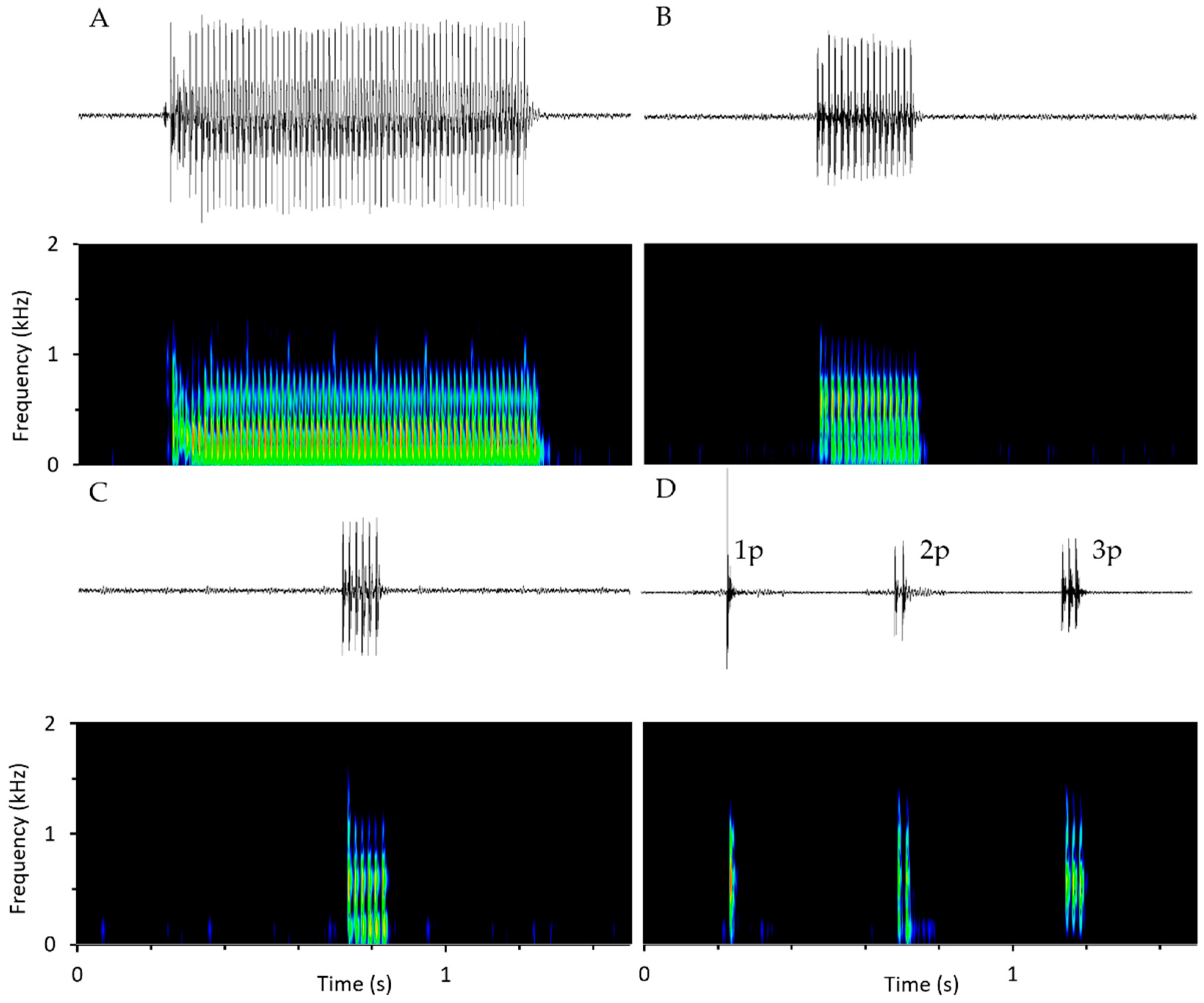
4.3.1. Sound Detection and Classification

Vocalizations were visually (spectrogram and oscillogram) and aurally detected on each file. Vocalizations were then classified into 6 different categories based on pulse number: Long grunts (more than 30 pulses; Figure 5A), intermediate grunts (7–29 pulses; Figure 5B), short grunts (4–6pulses; Figure 5C), 1 pulse, 2 pulses and 3 pulses (Figure 5D), and indeterminate sounds in cases in which the number of pulses could not be clearly determined since they presented an unclear pulsed structure in part of the sound. The latter could be caused by body movements of the vocalising fish. This classification attempted to include both the short and long grunt categories previously reported [20] and the calls that were registered in the present study.

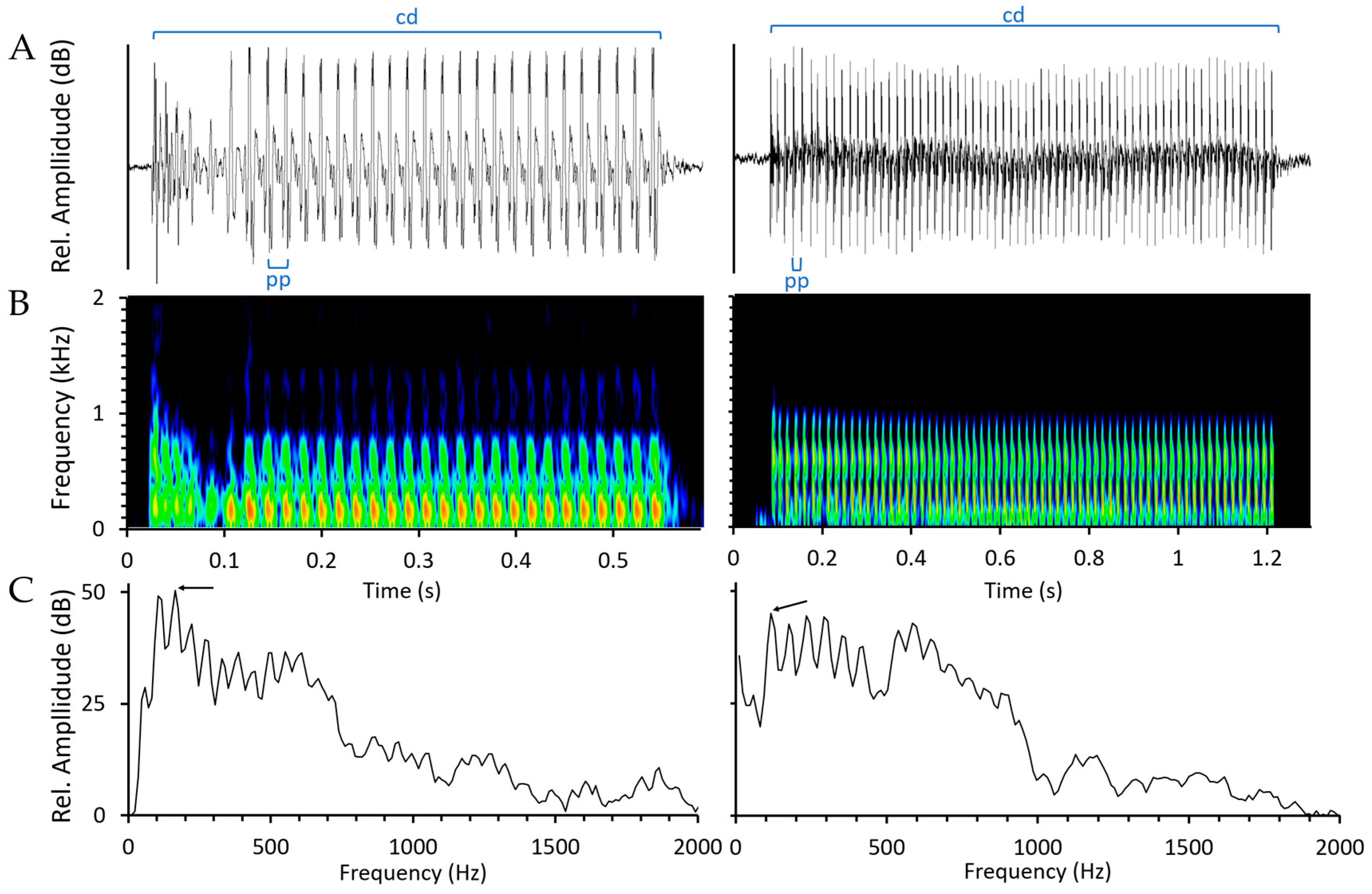
4.3.2. Acoustic Features Measurements

Temporal features and peak frequency were measured in the selected long grunts. Only sounds with a good signal-to-noise ratio recorded from the selected tank, which was equipped with a custom-made hydrophone [78], were used in the analyses. The following temporal and spectral parameters of sounds were measured: Call duration (ms), as the time from the onset of the first pulse to the offset of the last pulse; number of pulses, obtained manually by counting the number of pulses in each call; pulse period (ms) (the time interval between the peaks of two consecutive pulses in a call), obtained by dividing the duration by the number of pulses minus one; and peak frequency (Hz), the frequency presenting the highest energy level in the call. Temporal parameters were measured from oscillograms while peak frequency was measured from power spectra: 12 kHz, Fast Fourier Transform (FFT) size 1024 points, Hamming window, time overlap 50%. Calls presented several frequency peaks with similar energy (Figure 6). Consequently, the peak frequency corresponded to different frequency peaks in different calls due to small differences in relative energy imparting considerable variability to the data. See Figure 6 for the representation of some of the measured acoustic parameters.

4.4. Automatic Recognition

The proposed automatic recognition system was adapted from those described by Vieira and colleagues [15] using hidden Markov models (HMMs). For sound recognition, HMM is a statistical linear state model, where sequential states represent spectral configurations along time. Each HMM is characterized by the probabilities of transitioning from one state to the next, and the probabilities of a particular feature observation occurring while in each state. Briefly, multiple HMMs are trained using sounds of each defined category, the recordings being then classified according to the model with the highest likelihood. The overall flowchart of the method is shown in Figure 1 in [15].

4.4.1. Signal Processing

The waveform signal must be divided into a sequence of elementary segments according to a predefined window duration (see Figure 1, cf. [15]). This window should be longer than a cycle of the lower relevant frequency, but short enough to provide temporal resolution. After some preliminary tests, we chose a window of 32 ms with a 50% overlap to avoid losing information on the transition between two consecutive elementary segments [79]. We used the following acoustic features: Cepstrum, Mel-frequency cepstral (MFC), delta and acceleration coefficients. The selected frequency bandwidth ranged from 20 to 2000 Hz.

4.4.2. The HMM Time Alignment Structure

A human phoneme is usually modelled by three states [80]. However, because we do not have phonemes in fish calls, we assumed that the number of states should be equal to or higher than the number of different consecutive parts of the sound. Note that we used models with a linear topology in which all the states could transit to the same state, to the next or to the following one (except the initial and final states where self-transitions are meaningless as they only serve as signal boundary markers).

We created 4 models to classify the meagre call into different types based on pulse number: Long grunts (more than 30 pulses; Figure 5A), intermediate grunts (7–29 pulses; Figure 5B), short grunts (4–6 pulses; Figure 5C) and pulses (1 pulse, 2 pulses and 3 pulses; Figure 5D). After some preliminary tests, we considered 14 states for long grunts and intermediate grunts, 5 states for short grunts, pulses and background noise (silence) models. We added extra models with 5 states for modelling non-biological patterns with high energy and short duration (e.g., consecutive non-biological pulses with high energy).

For each sound type, a representative subset of samples was used to train the HMMs. The transition probabilities and the elementary segment probability densities of each state were estimated with the Baum–Welch algorithm [81].

In the recognition phase, each sound type was matched against the estimated HMM for each sound type. This was achieved by using a Viterbi algorithm [82] that produced a likelihood measure for each HMM.

For computations we used the HMM Toolkit (HTK, University of Cambridge, UK), a group of modules written in C to create automatic recognition systems for human speech [83].

4.4.3. System Training and Testing Process

An automatic HMM-based system was prepared to recognize and separate meagre calls into 4 different categories based on pulse number (long grunts, intermediate grunts, short grunts and pulses). The training set used to produce the recognition system included 129 meagre calls from a previously manually classified dataset of 222 calls (including indeterminate calls not used in the training) produced by fish housed in each tank. The system was tested with circa 18 hours of continuous recordings from 6 days (March 28th; April 18th and 28th, May 18th and 28th and June 18th) between 18:00 and 21:00.

4.4.4. Evaluation of the Recognition System

For each optimal alignment, the number of substitution errors (i.e., when one signal type is recognised as another signal type, S), deletion errors (i.e., when a sound type occurs but is not detected by the system—a false negative, D), insertion errors (i.e., when a signal is detected by the system but it did not occur—a false positive, I) and the total number of labels in the reference transcriptions (N) were determined (Young et al. 2000). The performance of the recognition systems was then evaluated by computing the percentage of correctly recognized sounds (identification rate) using:

$$\mathrm{Identification}\mathrm{rate}(\%)=\frac{\mathrm{N}-\mathrm{D}-\mathrm{S}}{\mathrm{N}}\times 100,$$

or by computing the recognition accuracy using:

$$\mathrm{Accuracy}(\%)=\frac{\mathrm{N}-\mathrm{D}-\mathrm{S}-\mathrm{I}}{\mathrm{N}}\times 100.$$

4.5. Analysis

4.5.1. Seasonal Changes in Calling Rate

The daily number of each type of vocalization was obtained both with manual and automatic methods. Using the automatic recognition system, we analysed all the round-the-clock recordings available from January 16 to the 14th of July 2018. No recordings were available from February 4 to 21 and April 24 to 27.

Through manual detection, we restricted the sampling effort to two days in each month, the 18th and 28th, between 18:00 and 21:00. A total of 7492 calls were manually counted.

4.5.2. Seasonal Changes in Calls Features

Temporal features and peak frequency were measured in 10 to 20 long grunts, excluding the calls with a low signal-to-noise ratio, randomly selected on two consecutive days of every month (depending on the presence/absence of calls) from March to July (March 27 and 28, April 29, May 18 and 19, June 4 and July 5 and 6). Long grunts were not detected in the periods sampled in February. The four temporal and spectral acoustic features measured were described above.

4.5.3. Diel Changes in Calling Rate

The numbers of each type of vocalization present in the recordings were obtained from the automatic recognition system. Using this system we counted the number of calls per hour in all round-the-clock recordings available from January to July 2018.

Preliminary visualization of calling activity suggested at least two types of rhythms depending on the overall daily number of calls. Thus, days were ranked by the number of calls detected in each day and classified in percentiles. Here we show the diel activity for the days under the 25th and over the 75th percentiles.

4.6. Statistical Analysis

Statistical analysis was conducted using the software Statistica (version 13, TIBCO Software Inc., Palo Alto, CA, USA). A P-level of 0.05 was used for all analyses [84]. Residual plots including probability plots, residual vs. predicted plots and Levene tests were performed to assess the normality of the data and the homogeneity of variances.

For the study of seasonal changes in sound features we tested whether temperature had a significant effect in long grunts’ acoustic variables with one-way analysis of covariance (ANCOVA). Water temperature was included as a continuous variable (covariate) because it can influence acoustic parameters [85]. When the effect of this covariate was not significant, one-way ANOVAs were conducted instead. The pulse period was log-transformed to meet the ANOVA assumptions. Homogeneity of variances assumptions were not met for peak frequency even after applying common data transformations [84]. In this case a non-parametric Kruskal-Wallis test was performed.

References

1. Winn, H.E. The biological significance of fish sounds. Mar. Bio-Acoust. 1964, 2, 213–231. [Google Scholar]
2. Connaughton, M.A.; Taylor, M.H. Seasonal and daily cycles in sound production associated with spawning in the weakfish, Cynoscion regalis. Environ. Biol. Fishes 1995, 42, 233–240. [Google Scholar] [CrossRef]
3. McCauley, R.D. Biological Sea Noise in Northern Australia: Patterns of Fish Calling. Ph.D. Thesis, James Cook University, Douglas, Australia, 2001. [Google Scholar]
4. Amorim, M.C.P. Diversity of sound production in fish. Commun. Fishes 2006, 1, 71–104. [Google Scholar]
5. McWilliam, J.N.; Hawkins, A.D. A comparison of inshore marine soundscapes. J. Exp. Mar. Biol. Ecol. 2013, 446, 166–176. [Google Scholar] [CrossRef]
6. Radford, C.A.; Jeffs, A.G.; Tindle, C.T.; Montgomery, J.C. Temporal patterns in ambient noise of biological origin from a shallow water temperate reef. Oecologia 2008, 156, 921–929. [Google Scholar] [CrossRef] [PubMed]
7. Radford, C.A.; Stanley, J.A.; Tindle, C.T.; Montgomery, J.C.; Jeffs, A.G. Localised coastal habitats have distinct underwater sound signatures. Mar. Ecol. Prog. Ser. 2010, 401, 21–29. [Google Scholar] [CrossRef]
8. Hawkins, A.D. The use of passive acoustics to identify a haddock spawning area. In Proceedings of the International Workshop on the Applications of Passive Acoustics to Fisheries, Cambridge, MA, USA, 8–10 April 2002. [Google Scholar]
9. Putland, R.L.; Ranjard, L.; Constantine, R.; Radford, C.A. A hidden Markov model approach to indicate Bryde’s whale acoustics. Ecol. Indic. 2018, 84, 479–487. [Google Scholar] [CrossRef]
10. Miller, B.S.; Miller, E.J. The seasonal occupancy and diel behaviour of Antarctic sperm whales revealed by acoustic monitoring. Sci. Rep. 2018, 8, 5429. [Google Scholar] [CrossRef] [PubMed]
11. Marques, T.A.; Thomas, L.; Martin, S.W.; Mellinger, D.K.; Ward, J.A.; Moretti, D.J.; Harris, D.; Tyack, P.L. Estimating animal population density using passive acoustics. Biol. Rev. Camb. Philos. Soc. 2013, 88, 287–309. [Google Scholar] [CrossRef] [PubMed]
12. Putland, R.L.; Mackiewicz, A.G.; Mensinger, A.F. Localizing individual soniferous fish using passive acoustic monitoring. Ecol. Inform. 2018, 48, 60–68. [Google Scholar] [CrossRef]
13. Parsons, M.J.; McCauley, R.D.; Mackie, M.C.; Siwabessy, P.; Duncan, A.J. Localization of individual mulloway (Argyrosomus japonicus) within a spawning aggregation and their behaviour throughout a diel spawning period. ICES J. Mar. Sci. 2009, 66, 1007–1014. [Google Scholar] [CrossRef]
14. Parsons, M.J.G.; McCauley, R.D.; Mackie, M.C.; Duncan, A.J. A Comparison of techniques for ranging close-proximity mulloway (Argyrosomus japonicus) calls with a single hydrophone. Acoust. Aust. 2010, 38, 145–151. [Google Scholar]
15. Vieira, M.; Fonseca, P.J.; Amorim, M.C.P.; Teixeira, C.J.C. Call recognition and individual identification of fish vocalizations based on automatic speech recognition: An example with the Lusitanian toadfish. J. Acoust. Soc. Am. 2015, 138, 3941–3950. [Google Scholar] [CrossRef]
16. Clemins, P.J.; Johnson, M.T.; Leong, K.M.; Savage, A. Automatic classification and speaker identification of African elephant (Loxodonta africana) vocalizations. J. Acoust. Soc. Am. 2005, 117, 956. [Google Scholar] [CrossRef]
17. Chou, C.H.; Lee, C.H.; Ni, H.W. Bird species recognition by comparing the HMMs of the syllables. In Proceedings of the Second International Conference on Innovative Computing, Informatio and Control (ICICIC 2007), Kumamoto, Japan, 5–7 September 2007; p. 143. [Google Scholar]
18. Parsons, M.J.G.; McCauley, R.D.; Mackie, M.C. Spawning sounds of the mulloway (Argyrosomus japonicus). In Proceedings of the ACOUSTICS, Christchurch, New Zealand, 20–22 November 2006. [Google Scholar]
19. Connaughton, M.A.; Taylor, M.H. Drumming, courtship, and spawning behavior in captive weakfish, Cynoscion regalis. Copeia 1996, 1996, 195–199. [Google Scholar] [CrossRef]
20. Lagardère, J.P.; Mariani, A. Spawning sounds in meagre Argyrosomus regius recorded in the Gironde estuary, France. J. Fish Biol. 2006, 69, 1697–1708. [Google Scholar] [CrossRef]
21. Montie, E.W.; Kehrer, C.; Yost, J.; Brenkert, K.; O’Donnell, T.; Denson, M.R. Long-term monitoring of captive red drum Sciaenops ocellatus reveals that calling incidence and structure correlate with egg deposition. J. Fish Biol. 2016, 88, 1776–1795. [Google Scholar] [CrossRef] [PubMed]
22. Montie, E.W.; Hoover, M.; Kehrer, C.; Yost, J.; Brenkert, K.; O’Donnell, T.; Denson, M.R. Acoustic monitoring indicates a positive relationship between calling frequency and spawning in captive spotted seatrout (Cynoscion nebulosus). PeerJ 2017, 5, e2944. [Google Scholar] [CrossRef]
23. Mok, H.-K.; Gilmore, R.G. Analysis of sound production in estuarine aggregations of Pogonias cromis, Bairdiella chrysoura, and Cynoscion nebulosus (Sciaenidae). Bull. Inst. Zool. Acad. Sin. 1983, 22, 157–186. [Google Scholar]
24. Saucier, M.H.; Baltz, D.M. Spawning site selection by spotted seatrout, Cynoscion nebulosus, and black drum, Pogonias cromis, in Louisiana. Environ. Biol. Fishes 1993, 36, 257–272. [Google Scholar] [CrossRef]
25. Luczkovich, J.J.; Daniel, H.J.; Sprague, M.W.; Johnson, S.E. Characterization of Critical Spawning Habitats of Weakfish, Spotted Seatrout and Red Drum In Pamlico Sound Using Hydrophone Surveys; North Carolina Department of Environment and Natural Resources: Morehead City, NC, USA, 1999. [Google Scholar]
26. Quéméner, L.; Suquet, M.; Mero, D.; Gaignon, J.-L. Selection method of new candidates for finfish aquaculture: The case of the French Atlantic, the Channel and the North Sea coasts. Aquat. Living Resour. 2002, 15, 293–302. [Google Scholar] [CrossRef]
27. Reynolds, D.; Rose, R. Robust text-independent speaker identification using Gaussian mixture speaker models. IEEE Trans. Speech Audio Proc. 1995, 3, 72–83. [Google Scholar] [CrossRef]
28. Lippmann, R.P. An introduction to computing with neural nets. IEEE ASSP Mag. 1987, 4, 4–22. [Google Scholar] [CrossRef]
29. Yu, H.; Oh, Y. A neural network for 500 vocabulary word spotting using acoustic sub-word units. In Proceedings of the 1997 IEEE International Conference on Acoustics, Speech, and Signal Processing, Munich, Germany, 21–24 April 1997; pp. 3277–3280. [Google Scholar]
30. Baker, J. The DRAGON system—An overview. Acoust. Speech Signal Process. IEEE Trans. 1975, 23, 24–29. [Google Scholar] [CrossRef]
31. Jelinek, F. Continuous speech recognition by statistical methods. Proc. IEEE 1976, 64, 532–556. [Google Scholar] [CrossRef]
32. Jelinek, F.; Bahl, L.; Mercer, R. Design of a linguistic statistical decoder for the recognition of continuous speech. IEEE Trans. Inf. Theory 1975, 21, 250–256. [Google Scholar] [CrossRef]
33. Rabiner, L.R. A tutorial on hidden Markov models and selected applications in speech recognition. Proc. IEEE 1989, 77, 257–286. [Google Scholar] [CrossRef]
34. Young, S.; Bloothooft, G. Corpus-Based Methods in Language and Speech Processing; Kluwer Academic Publishers: Dordrecht, The Netherlands, 1997. [Google Scholar]
35. Tellechea, J.S.; Fine, M.L.; Norbis, W. Passive acoustic monitoring, development of disturbance calls and differentiation of disturbance and advertisement calls in the A rgentine croaker U mbrina canosai (S ciaenidae). J. Fish Biol. 2017, 90, 1631–1643. [Google Scholar] [CrossRef]
36. Sattar, F.; Cullis-Suzuki, S.; Jin, F. Identification of fish vocalizations from ocean acoustic data. Appl. Acoust. 2016, 110, 248–255. [Google Scholar] [CrossRef]
37. Ibrahim, A.K.; Chérubin, L.M.; Zhuang, H.; Schärer Umpierre, M.T.; Dalgleish, F.; Erdol, N.; Ouyang, B.; Dalgleish, A. An approach for automatic classification of grouper vocalizations with passive acoustic monitoring. J. Acoust. Soc. Am. 2018, 143, 666–676. [Google Scholar] [CrossRef]
38. Monczak, A.; Ji, Y.; Soueidan, J.; Montie, E.W. Automatic detection, classification, and quantification of sciaenid fish calls in an estuarine soundscape in the Southeast United States. PLoS ONE 2019, 14, e0209914. [Google Scholar] [CrossRef]
39. Noda, J.; Travieso, C.; Sánchez-Rodríguez, D. Automatic taxonomic classification of fish based on their acoustic signals. Appl. Sci. 2016, 6, 443. [Google Scholar] [CrossRef]
40. Lin, T.-H.; Tsao, Y.; Akamatsu, T. Comparison of passive acoustic soniferous fish monitoring with supervised and unsupervised approaches. J. Acoust. Soc. Am. 2018, 143, EL278–EL284. [Google Scholar] [CrossRef]
41. Harakawa, R.; Ogawa, T.; Haseyama, M.; Akamatsu, T. Automatic detection of fish sounds based on multi-stage classification including logistic regression via adaptive feature weighting. J. Acoust. Soc. Am. 2018, 144, 2709–2718. [Google Scholar] [CrossRef] [PubMed]
42. Malfante, M.; Mars, J.I.; Dalla Mura, M.; Gervaise, C. Automatic fish sounds classification. J. Acoust. Soc. Am. 2018, 143, 2834–2846. [Google Scholar] [CrossRef] [PubMed]
43. Potter, J.; Mellinger, D.; Clark, C. Marine mammal call discrimination using artificial neural networks. J. Acoust. Soc. Am. 1994, 96, 1255. [Google Scholar] [CrossRef]
44. Murray, S.; Mercado, E.; Roitblat, H. The neural network classification of false killer whale (Pseudorca crassidens) vocalizations. J. Acoust. Soc. Am. 1998, 104, 3626. [Google Scholar] [CrossRef]
45. Schaar, M. van der Neural network-based sperm whale click classification. J. Mar. Biol. Assoc. UK 2007, 87, 35. [Google Scholar] [CrossRef]
46. Pace, F.; White, P.; Adam, O. Hidden Markov Modeling for humpback whale (Megaptera Novaeanglie) call classification. Proc. Meetings Acoust. 2012, 17, 070046. [Google Scholar]
47. Gillespie, D.; Caillat, M.; Gordon, J.; White, P. Automatic detection and classification of odontocete whistles. J. Acoust. Soc. Am. 2013, 134, 2427–2437. [Google Scholar] [CrossRef]
48. Peso Parada, P.; Cardenal-López, A. Using Gaussian mixture models to detect and classify dolphin whistles and pulses. J. Acoust. Soc. Am. 2014, 135, 3371–3380. [Google Scholar] [CrossRef]
49. Lin, T.-H.; Chou, L.-S. Automatic classification of delphinids based on the representative frequencies of whistles. J. Acoust. Soc. Am. 2015, 138, 1003–1011. [Google Scholar] [CrossRef]
50. Erbs, F.; Elwen, S.H.; Gridley, T. Automatic classification of whistles from coastal dolphins of the southern African subregion. J. Acoust. Soc. Am. 2017, 141, 2489–2500. [Google Scholar] [CrossRef] [PubMed]
51. Jiang, J.; Bu, L.; Wang, X.; Li, C.; Sun, Z.; Yan, H.; Hua, B.; Duan, F.; Yang, J. Clicks classification of sperm whale and long-finned pilot whale based on continuous wavelet transform and artificial neural network. Appl. Acoust. 2018, 141, 26–34. [Google Scholar] [CrossRef]
52. Campbell, G.; Gisiner, R.; David, A.; Milette, L. Acoustic identification of female Steller sea lions (Eumetopias jubatus). J. Acoust. Soc. Am. 2002, 101, 2920–2928. [Google Scholar] [CrossRef]
53. Guest, W.C.; Lasswell, J.L. A note on courtship behavior and sound production of red drum. Copeia 1978, 1978, 337–338. [Google Scholar] [CrossRef]
54. Luczkovich, J.J.; Sprague, M.W.; Johnson, S.E.; Pullinger, R.C. Delimiting spawning areas of weakfish Cynoscion regalis (family Sciaenidae) in Pamlico Sound, North Carolina using passive hydroacoustic surveys. Bioacoustics 1999, 10, 143–160. [Google Scholar] [CrossRef]
55. McIver, E.L.; Marchaterre, M.A.; Rice, A.N.; Bass, A.H. Novel underwater soundscape: Acoustic repertoire of plainfin midshipman fish. J. Exp. Biol. 2014, 217, 2377–2389. [Google Scholar] [CrossRef] [PubMed]
56. Fish, J.F.; Cummings, W.C. A 50-dB increase in sustained ambient noise from fish (Cynoscion xanthulus). J. Acoust. Soc. Am. 1972, 52, 1266–1270. [Google Scholar] [CrossRef]
57. Takemura, A.; Takita, T.; Mizue, K. Studies on the underwater sound, 7: Underwater calls of the Japanese marine drum fishes (Sciaenidae). Bull. Jpn. Soc. Sci. Fish. 1978, 54, 21–27. [Google Scholar]
58. Parsons, M.J.G.; McCauley, R.D.; Mackie, M.C. Characterisation of mulloway argyrosomus japonicus advertisement sounds. Acoust. Aust. 2013, 41, 196–201. [Google Scholar]
59. Borie, A.; Mok, H.-K.; Chao, N.L.; Fine, M.L. Spatiotemporal variability and sound characterization in Silver Croaker Plagioscion squamosissimus (Sciaenidae) in the Central Amazon. PLoS ONE 2014, 9, e99326. [Google Scholar] [CrossRef]
60. Feher, J.J.; Waybright, T.D.; Fine, M.L. Comparison of sarcoplasmic reticulum capabilities in toadfish (Opsanus tau) sonic muscle and rat fast twitch muscle. J. Muscle Res. Cell Motil. 1998, 19, 661–674. [Google Scholar] [CrossRef] [PubMed]
61. Ladich, F. Acoustic communication in fishes: Temperature plays a role. Fish Fish. 2018, 19, 598–612. [Google Scholar] [CrossRef]
62. Vicente, J.R.; Fonseca, P.J.; Amorim, M.C.P. Effects of temperature on sound production in the painted goby Pomatoschistus pictus. J. Exp. Mar. Biol. Ecol. 2015, 473, 1–6. [Google Scholar] [CrossRef]
63. Bass, A.H.; Baker, R. Sexual dimorphisms in the vocal control system of a teleost fish: Morphology of physiologically identified neurons. J. Neurobiol. 1990, 21, 1155–1168. [Google Scholar] [CrossRef]
64. Fine, M.L. Seasonal and geographical variation of the mating call of the oyster toadfish Opsanus tau L. Oecologia 1978, 36, 45–57. [Google Scholar] [CrossRef] [PubMed]
65. Torricelli, P.; Lugli, M.; Pavan, G. Analysis of sounds produced by male Padogobius martensi (Pisces, Gobiidae) and factors affecting their structural properties. Bioacoustics 1990, 2, 261–275. [Google Scholar] [CrossRef]
66. Brantley, R.K.; Bass, A.H. Alternative male spawning tactics and acoustic signals in the plainfin midshipman fish Porichthys notatus Girard (Teleostei, Batrachoididae). Ethology 1994, 96, 213–232. [Google Scholar] [CrossRef]
67. Connaughton, M.A.; Taylor, M.H.; Fine, M.L. Effects of fish size and temperature on weakfish disturbance calls: Implications for the mechanism of sound generation. J. Exp. Biol. 2000, 203, 1503–1512. [Google Scholar] [PubMed]
68. Holt, S.A.; Holt, G.J. Effects of variable salinity on reproduction and early life stages of spotted seatrout. In Biology of the Spotted Seatrout; CRC Press: Boca Raton, FL, USA, 2002; pp. 140–150. [Google Scholar]
69. Holt, G.J.; Holt, S.A.; Arnold, C.R. Diel periodicity of spawning in sciaenids. Mar. Ecol. Prog. Ser. 1985, 27, 7. [Google Scholar] [CrossRef]
70. Montie, E.W.; Vega, S.; Powell, M. Seasonal and spatial patterns of fish sound production in the May River, South Carolina. Trans. Am. Fish. Soc. 2015, 144, 705–716. [Google Scholar] [CrossRef]
71. Middaugh, D.P. Reproductive ecology and spawning periodicity of the Atlantic silverside, Menidia menidia (Pisces: Atherinidae). Copeia 1981, 766–776. [Google Scholar] [CrossRef]
72. Doherty, P.J. Diel, lunar and seasonal rhythms in the reproduction of two tropical damselfishes: Pomacentrus flavicauda and P. wardi. Mar. Biol. 1983, 75, 215–224. [Google Scholar] [CrossRef]
73. Hobson, E.S.; Chess, J.R. Trophic relationships among fishes and plankton in the lagoon at Enewetak Atoll, Marshall Island. Fish. Bull 1978, 76, 133–153. [Google Scholar]
74. Lobel, P.S. Diel, lunar, and seasonal periodicity in the reproductive behavior of the pomacanthid fish, Centropyge potteri, and some other reef fishes in Hawaii. Pac. Sci. 1978, 32, 193–207. [Google Scholar]
75. Ferraro, S.P. Daily time of spawning of 12 fishes in the Peconic Bays, New York, USA. Fish. Bull. US 1980, 78, 455–464. [Google Scholar]
76. Robertson, D.R. On the spawning behavior and spawning cycles of eight surgeonfishes (Acanthuridae) from the Indo-Pacific. Environ. Biol. Fishes 1983, 9, 193–223. [Google Scholar] [CrossRef]
77. Amorim, M.C.P.; Hawkins, A.D. Growling for food: Acoustic emissions during competitive feeding of the streaked gurnard. J. Fish Biol. 2000, 57, 895–907. [Google Scholar] [CrossRef]
78. Fonseca, P.J.; Maia Alves, J. Electret Capsule Hydrophone: A New Underwater Sound Detector. Patent Application PT105, 2011. [Google Scholar]
79. O’shaughnessy, D. Speech Communication: Human and Machine; Addison-Wesley: Boston, MA, USA, 1987. [Google Scholar]
80. McDermott, E.; Iwamida, H.; Katagiri, S.; Tohkura, Y. Shift-tolerant LVQ and hybrid LVQ-HMM for phoneme recognition. In Readings in Speech Recognition; Morgan Kaufmann Publishers: San Mateo, CA, USA, 1990; pp. 425–438. [Google Scholar]
81. Baum, L.; Petrie, T.; Soules, G.; Weiss, N. A maximization technique occurring in the statistical analysis of probabilistic functions of Markov chains. Ann. Math. Stat. 1970, 41, 164–171. [Google Scholar] [CrossRef]
82. Forney, G. The viterbi algorithm. Proc. IEEE 1973, 6, 268–278. [Google Scholar] [CrossRef]
83. Young, S.; Evermann, G.; Gales, M. The HTK Book Version 3.4; Cambridge University Press: Cambridge, UK, 2006. [Google Scholar]
84. Zar, J.H. Biostatistical Analysis Englewood Cliffs; Prentice-Hall: New York, NY, USA, 1984; p. 360. [Google Scholar]
85. Amorim, M.C.P.; Vasconcelos, R.O.; Marques, J.F.; Almada, F. Seasonal variation of sound production in the Lusitanian toadfish Halobatrachus didactylus. J. Fish Biol. 2006, 69, 1892–1899. [Google Scholar] [CrossRef]
Figure 1. Proportion of sound categories from 3-hour recordings, between 18:00 and 21:00, in two days per month in the peak of the spawning season. (A) The automatic classification and (B) the manual classification.
Fishes 04 00028 g001
Figure 2. Seasonal variation of (A) the number of calls per day, (B) the mean number of calls per month, (C) the proportion of sound categories identified by the automatic recognition system, (D) the number of days with spawning events per month, (E) the eggs’ total weight and (F) mean water temperature per month. A total of 7492 calls were counted and categorized manually from 3-h recordings, between 18:00 and 21:00, in two days per month, from January to June 2018. The values obtained with the automatic recognition system represent monthly means of the calls counted on the full round-the-clock recordings. Notice that in (A) the horizontal axis is a continuous scale of days at each month. In addition, note that spawning (D and E) occurs in discrete events.
Fishes 04 00028 g002
Figure 3. Seasonal variation of (A) sound duration (ms), (B) pulse period (ms), (C) number of pulses and (D) peak frequency (Hz) of long grunts (10 to 20 calls were considered per month). In (AC) mean and 95% confidence intervals are shown. In the case of pulse periods, the mean and confidence intervals were computed for covariate at their mean (20.5 °C). In (D) median, quartiles and range are shown. In red, water temperature variation (mean values on the selected days, ˚C).
Fishes 04 00028 g003
Figure 4. Diel variation of call rate (A) at all sampled days, (B) at the days with high calling activity (>the 75th percentile) and (C) at the days with low calling activity (<the 25th percentile). The values obtained from the automatic recognition represent a mean of the calls counted per hour; (A) depicts mean and standard error of calling rate. Notice that the (C) vertical axis is in different scales.
Fishes 04 00028 g004
Figure 5. Oscillograms and spectrograms representing meagre’s acoustic repertoire: (A) Long grunts (30–135 pulses), (B) intermediate grunts (7–29 pulses), (C) short grunts (4–6pulses) and (D) 1, 2 and 3 pulses. Sampling frequency 12 kHz, 1024 point FFT, 98 points window, Hamming window, and 50% overlap.
Fishes 04 00028 g005
Figure 6. (A) Oscillograms, (B) spectrograms and (C) power spectra of two Argyrosomus regius male breeding calls, representing some of the measured acoustic parameters: (pp) Pulse period and (cd) call duration in (A), and peak frequency (arrow) in (C). Sampling frequency 12 kHz, 1024 point FFT, 98 points window, Hamming window and 50% overlap. Note differences in call duration and power spectra between calls. The call on the left also shows variability in pulse rate and amplitude modulation.
Fishes 04 00028 g006