Article

Studying Kenai River Fisheries’ Social-Ecological Drivers Using a Holistic Fisheries Agent-Based Model: Implications for Policy and Adaptive Capacity

1
Software Engineer, General Communications Inc., Anchorage, AK 99503, USA
2
Computer Science, University of Portland, Portland, OR 97203, USA
3
Environmental Science and Policy, Southern Oregon University, Ashland, OR 97520, USA
*
Author to whom correspondence should be addressed.
Submission received: 20 March 2019 / Revised: 12 May 2019 / Accepted: 27 May 2019 / Published: 31 May 2019
(This article belongs to the Special Issue Climate Change on Fish and Fisheries)

Abstract

:
Alaska’s salmon fisheries are one of the more intensely managed natural resources in the world. The state’s salmon fisheries support recreational, subsistence, and commercial harvest with multiple billions of dollars flowing into the economy, and define the cultural identity of many Alaskans. Fishery management practices rely on historic records to set policies with two goals: to meet salmon escapement quota and to maximize salmon harvest. At the same time, rapid social and ecological changes to the sub-Arctic are already impacting salmon runs and fisheries management. Combined with the inability of fishery managers to test the outcome of proposed policy changes, an understanding of the role social and ecological drivers play in harvest and effort is required. To address the two-forked problem of understanding socio-ecological dynamics and potential policy responses to ecological and social changes, we (1) conducted stakeholder workshops to solicit key system drivers, (2) built an integrated agent based model (ABM) of the system’s socio-ecological dynamics, and (3) tested the impacts of alternative future scenarios of ecological, social, and policy changes on the system’s outcomes. We previously constructed and validated a high-fidelity, data-driven, agent-based model of the Kenai River, Alaska that simulates seasonal harvest of sockeye and Chinook salmon, the fishing activities of the personal use fishery, commercial drift, and set gillnet agents. We study the role of key stakeholder and ecological drivers, using the ABM decision support tool, and their implications for fisheries management policies. Analysis of the scenario based studies found resilience in management of commercial fisheries to changing salmon migration dynamics, a lack of adaptive capacity in recreational (personal use) dipnet users to altered sockeye salmon runs, and the possible utility of introducing management measures in the dipnet fishery to manipulate sockeye escapement levels. These findings represent the usefulness of this type of ABM in assisting fishery managers everywhere in investigating possible future outcomes of different management or ecological scenarios.

1. Introduction

The harvest of Alaska salmon fisheries has been consistently high since the 1990s, with annual salmon harvest of commercial fisheries exceeding 100 million salmon every year since 1987 [1,2]. Repeated high sustainable yield has been attributed to active management practices by a single state management agency, the Alaska Department of Fish and Game (ADFG) [2,3]. Their approach of emergency restricting or permitting fisheries gear and openings based on escapement is scientifically grounded and focused on fisheries sustainability. The success of their sustainable fisheries management approach can also be seen in the Bristol Bay fishery, where over 10 million sockeye salmon have been harvested since 1995 [4,5]. The abundance of Alaska’s salmon fisheries support large numbers of commercial and personal use fishermen, provide subsistence resource for remote communities, and define recreational and cultural identity of many Alaskans.
The returning salmon runs in Southcentral Alaska’s Upper Cook Inlet support commercial drift gillnet and set gillnet fisheries, as well as personal use, sport fishing, and subsistence fisheries [6]. Sockeye are the heart of the salmon fishery thanks to the returning 20-year average annual runs of 3 . 7 million sockeye that yield commercial fishery harvests in excess of 2 million sockeye salmon annually, as well as sport and personal use fishery harvests frequently in excess of 300,000 fish [7]. To maintain the high volume of salmon runs, ADFG manages the salmon fisheries for optimal sustainable salmon escapement quota. The escapement goal is determined by historical harvest and returns, as well as the best available biological data [8,9].

1.1. Identifying Socio-Ecological Drivers through Stakeholder Workshops

Policy-relevant socio-ecological system (SES) drivers were identified from participatory scenario planning (PSP) workshops where cumulative stressors were decomposed into individual drivers of change [10]. PSP informs resource management by evaluating alternative scenarios of SES changes to build a common understanding about the systems dynamics [11]. The first workshop identified drivers of change that include (a) past, present, and future decisions, (b) critical uncertainties [12], and (c) key actors in the region that may influence the decisions and uncertainties. Participants first identified the key decisions that have, and will continue to influence the region through a series of individual and group exercises. Then participants narrowed-in on six critical uncertainties that are likely to significantly impact salmon management in the Kenai river basin, based on those decisions that could be made. The six critical uncertainties include: climate warming impacts to freshwater systems, changing marine systems limiting food for salmon, land and natural gas development being favored over salmon habitat protection, regional population growth leading to increased fishing and land competition, increases in sport fishing user days, and increases in personal use fishery participation. The five primary stakeholders (Alaska Department of Fish & Game, Alaska Department of Natural Resources, Kenai Peninsula Borough, Kenai Watershed Forum, Kenai Wildlife Refuge) and the additional 28 emerging key actors in the region were then identified, ranked, and linked to the uncertainties to highlight decision points. The overarching themes of the past, present, and future decisions to be made included: uncertainty of the climate future and management decisions; make habitat conservation a priority; promote inter-agency cooperation to create a watershed plan with pooled resources and planning processes; loss of freshwater habitat, increased stream temperatures, increased sedimentation, changing hydrological regimes, increase in invasive species, increase in disease; new economic pressures; salmon protection compensation; lack of fish due to changing marine conditions, acidification of currents; increased demand for the land and anthropogenic resources that negatively effect the fish resources; population increase resulting in a sport fisherman user days increase; increasing participation in the personal user fishery. (For more details on the workshops’ findings, including a social network analysis of the stakeholders, as well as the complete list of the past, present, and future decisions, please see the workshop website and associated publications [13,14,15].) Together, these represent robust SES drivers that then informed definition of stakeholder-defined scenarios [15] as well as ABM scenarios, described below.

1.1.1. Chinook By-Catch Driver

In contrast to the Kenai River’s high volume of returning sockeye salmon, the watershed is also a productive habitat for an annual return of approximately 50,000 Chinook salmon. Chinook return for spawning between July and the end of August, at the same time as the much larger sockeye run [16]. Due to long-term Chinook stock decline, regulations prohibit targeted commercial harvest, and limit the personal use harvest of this prized sport salmon species. Satisfying the Chinook escapement goals is complicated by the small run size (relative to the sockeye); the reported Chinook by-catch by the commercial set gillnet fishery alone averages 9452 since 1966 [7]. In some years, the high Chinook by-catch prompts in-season fishing restrictions and fishery closures by ADFG to meet the Chinook escapement goals [17,18]. To minimize Chinook by-catch, proposed policies include reducing set gillnet net depth, as the Chinook migrate at deeper parts of the water column. If reducing Chinook by-catch is effective, the gillnet commercial fisheries would face less restrictions, increasing their potential sockeye harvest, while maintaining the Chinook escapement goals

1.1.2. Personal Use Fisheries Participation Driver

The large annual sockeye harvest from commercial fisheries makes them an effective tool to control salmon escapement during periods of increased salmon return [19]. The other participating fisheries are not as actively managed to control the escapement goal. However, the personal use fishery effort, often simply called the “dipnet” fishery, has more than tripled since the fishery first opened in 1996, going from 10,503 dipnet days fished to a record breaking 36,383 dipnet days fished in 2014 [7]. Dipnet sockeye harvest has correspondingly increased from approximately 100,000–200,000 salmon in the mid-late 1990s to 300,000–500,000 between 2011–2017 [7]. The increasing impact of the dipnet fishery on sockeye escapement is causing it to be considered for future active management interventions to increase or decrease sockeye escapement as required [20].

1.1.3. Run-Timing Dynamics Driver

In addition to anticipated changes in social drivers, the effects of climate change were reported to significantly alter the migration timing of returning salmon, potentially effecting both stakeholder harvest and salmon escapement [21,22,23]. Kovach et al. reported that the majority of sockeye and Chinook populations in Southeast Alaska were migrating later, and they linked these migration shifts to climatic changes [21]. The seasonal variation in migration timings were highly variable across the species, but can be attributed to the climate variability on the large scale—Pacific Decadal Oscillation (PDO), the meso-scale—sea surface, hydrology, and nutrient availability, as well as the micro-scale—precipitation. The authors also observed that the duration of some salmon runs are extended, or shortened, by up to two weeks without changes to overall abundance [21]. In Southcentral Alaska, the average Chinook size has been steadily decreasing since the overfishing in the 1980s and the increased glacier runoff due to the increased ambient temperatures. The combination of the ongoing changes, the observed changes in dynamics in Southeast Alaska, and the local-scale climate variability (in the stream temperatures for example) justify the configuration of the run-timing scenarios with up to two weeks earlier or later shifts in the migration dynamics. The temporal alignment between the migration run and the dipnet fishery season, set from 10 July–31 July, could result in a substantially reduced dipnet harvest if the peak of the run is outside of the fishing season.

1.1.4. ADFG Management Dynamics Driver

ADFG’s fisheries management decisions integrate scientific, historical, stakeholder data, including genetic stock identification, test fisheries for run predictions, sonar devices for in-river salmon counts, and fisheries harvest data, to name a few [6,24]. The diverse information sources and modeling tools help ADFG select the best trade-off option in response to the changing run conditions. However sophisticated the decision making process is, ADFG does not have the tools to a priori test the outcome of proposed policy changes on the SES dynamics. The implementation of an untested policy change carries uncertainty about its effectiveness or consequences. As a result, the ability of fishery managers to pro-actively manage fisheries is less than ideal. Fishery managers can better anticipate future social or ecological changes by using models constructed to study the impact of climate change on subsistence fishing as well as fishing profitability, and how altered social drivers (fishing area, effort) might effect fisheries and their ecosystem [25,26,27].

2. Methods

We previously designed and validated an open source high-fidelity, data-driven agent-based model (ABM) for simulating socio-ecological dynamics of Pacific salmon fisheries at the Kenai River [28,29]. The ABM is available for download for those who would like to inspect it [30]. The ABM simulates returning Chinook and sockeye salmon runs and the fishing effort of three user groups attempting to harvest the salmon during a season. In addition to the two salmon species as agent types, the model includes fishermen agents representing personal use, commercial set gillnet, and commercial drift gillnet fisheries. Using our ABM, we tested a total of 28 different scenarios that explore different combinations of set gillnet net depth and length, dipnet effort and dipnet net width, and median date of migration timing (MDMT) and duration of migration timing (DMT) for returning Chinook and sockeye, and quantify the impact in terms of returning salmon for spawning. Throughout all of these scenarios, our model simulated the management dynamics currently in play at the fisheries today via emergency closures and openings for the gillnet fisheries, gear restrictions for dipnetters and gillnetters, fishery location restrictions and regulations, and season openings and closings.

2.1. Model Summary

The model simulates socio-ecological dynamics of an annual fishing season from mid-June to mid-September with returning runs of sockeye and Chinook salmon and the fishing seasons of three user groups. Table 1 shows the key model parameters that drive the social and ecological dynamics while Figure 1 shows the simulated watershed and the stakeholder fishing zones in the model (For the details of the model construction, model validation and behavior analysis please see [28,29].

2.2. Studied Scenarios

Default simulation values in Table 1 were altered to study a set of scenarios representing plausible combinations of social and environmental change in the management of the Kenai River (see Table 2)

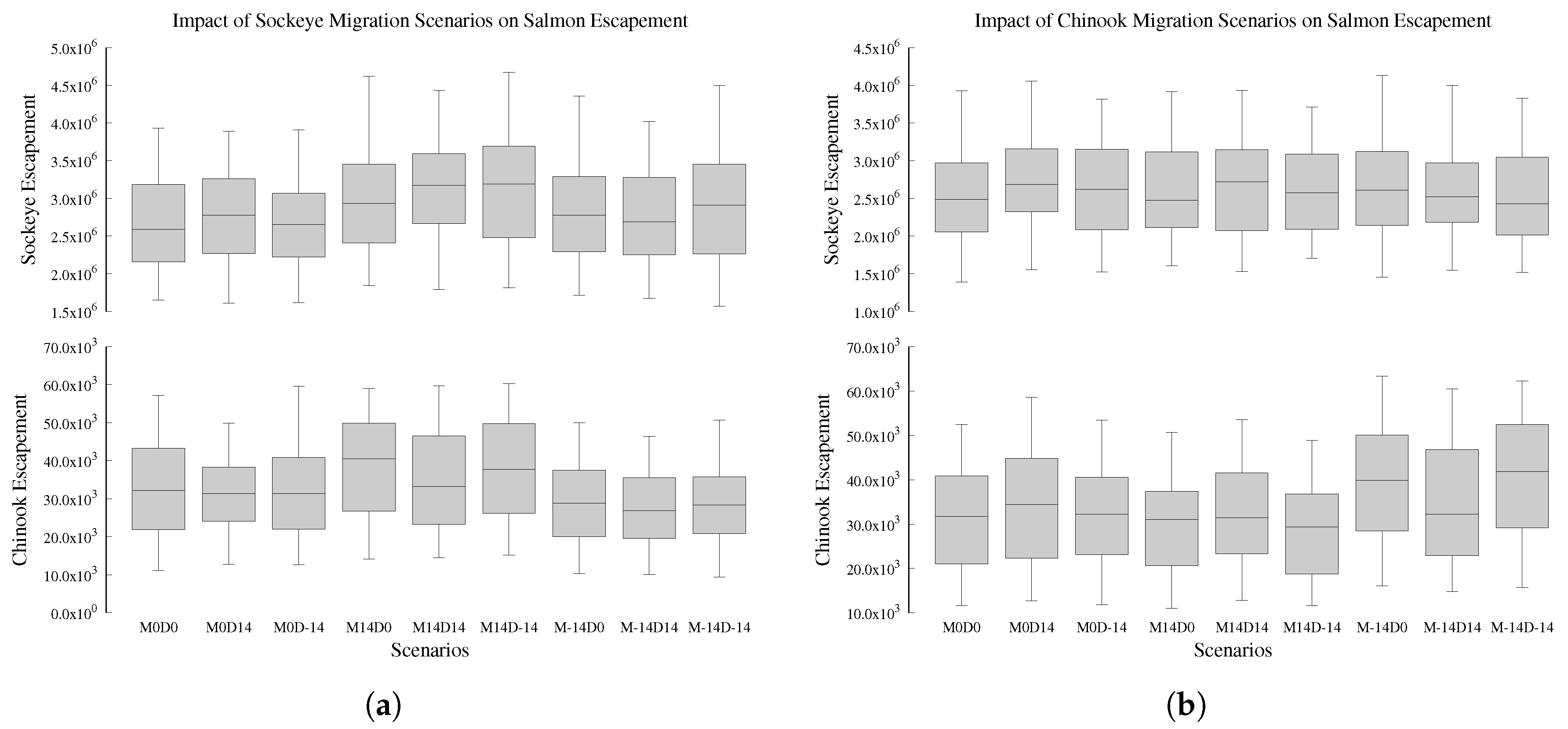
2.2.1. Sockeye and Chinook Migration Scenarios

The sockeye migration and Chinook migration scenarios in Table 2 show the range of possible values for sockeye and Chinook DMT and MDMT under their respective scenarios tested.
Figure 2 illustrates the construction of DMT and MDMT scenarios with respect to the original migration distribution. Note that the seasonal salmon abundance is unchanged, only the migration distribution is altered as observed by Kovach et al. in Southeast Alaska fisheries [21].

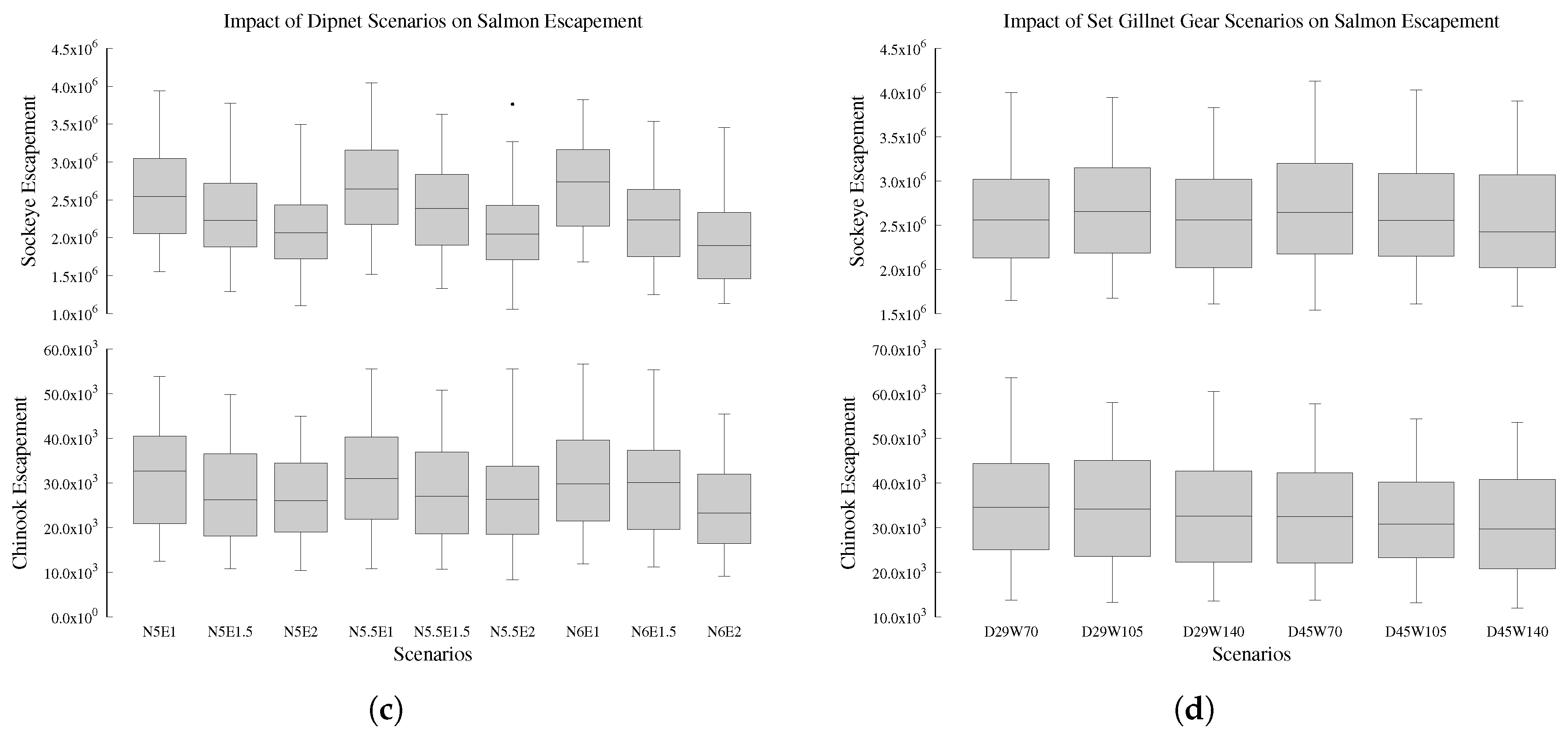
2.2.2. Set Gillnet Gear Scenarios

Chinook by-catch has been particularly impacted by set gillnet net depth, since Chinook migrate at deeper depths in the water column than sockeye salmon [6,18]. Welch et al. modeled the probability of harvesting sockeye and Chinook salmon as a function of set gillnet net depth based on migration depth distributions calculated from telemetry data [18].
Regulations permit set gillnet net depth and net width to extend to 45 meshes deep (6 in. per mesh) and 105 fathoms in length (6 ft. per fathom) [31]. Welch et al. showed that reducing net depth to 29 meshes and extending net length to 140 fathoms could reduce Chinook by-catch while maintaining levels of sockeye harvest [18]. The ABM was used to test alterations in set gillnet depth and width in order to extend their work to account for how other drivers might influence the impact of gear alteration on sockeye and Chinook harvest (Table 2).

2.2.3. Dipnet Participation and Gear Scenarios

Scenarios investigating increasing dipnet effort and gear width reflect the increasing interest in the dipnet fishery, and aim to study (1) how the dipnet fishery and other fisheries’ harvest could be effected by significant changes in the dipnet fishery dynamics, and (2) the potential for the dipnet fishery to be actively managed to meet salmon escapement goals.
The Dipnet Effort Adjust parameter in Table 1 was used to alter the control values for dipnet effort from our model validation. Additionally, alterations to dipnet width were tested to determine impact on sockeye harvest similar to the set gillnet gear scenarios. Possible parameter values for dipnet gear and effort scenarios are in Table 2.

2.3. Scenario Analysis and Cost of Outcomes

Due to stochastic construction of the ABM, each scenario was independently executed 133 times with a randomly generated seed for statistical significance of measured output dynamics [32]. Response variables for each scenario were analyzed by a one-way analysis-of-variance (ANOVA) model [33]. Response variables of fishermen salmon harvest by fishery and species, fishermen effort, and salmon escapement by species were used. The research hypothesis for the response variables was H a : μ c μ j for control scenario c, and some scenario j. The null hypothesis was H o : μ c = μ j for control scenario c, and all scenarios j. These hypotheses were applied to each of the scenario groupings in Table 2. Each scenario used Tukey’s Honest Significant Difference (HSD) test to determine significant differences in response variables. A critical level of α = 0 . 001389 was used for hypothesis testing. The parameter sensitivity of the SES dynamics was visualized through box-plots of stakeholder harvest and effort for each scenario. Stakeholder sockeye harvest was also converted to ex-vessel revenue to illustrate the direct economic impact under the simulated scenarios. The ex-vessel value of $ 1 . 05 lb−1 and average sockeye salmon weight of 5 . 8 lb for the 2016 central district Upper Cook Inlet fisheries were used for conversion of simulated stakeholder sockeye harvest to ex-vessel values [1,34].

3. Results and Discussion

Significant differences in stakeholder sockeye harvest and effort were detected for sockeye migration, dipnet gear and effort, and set gillnet gear scenarios (Table A1). No significant differences in sockeye harvest or effort were found for any of the Chinook migration scenarios (please see Figure A1 in Appendix A.2 for more details).

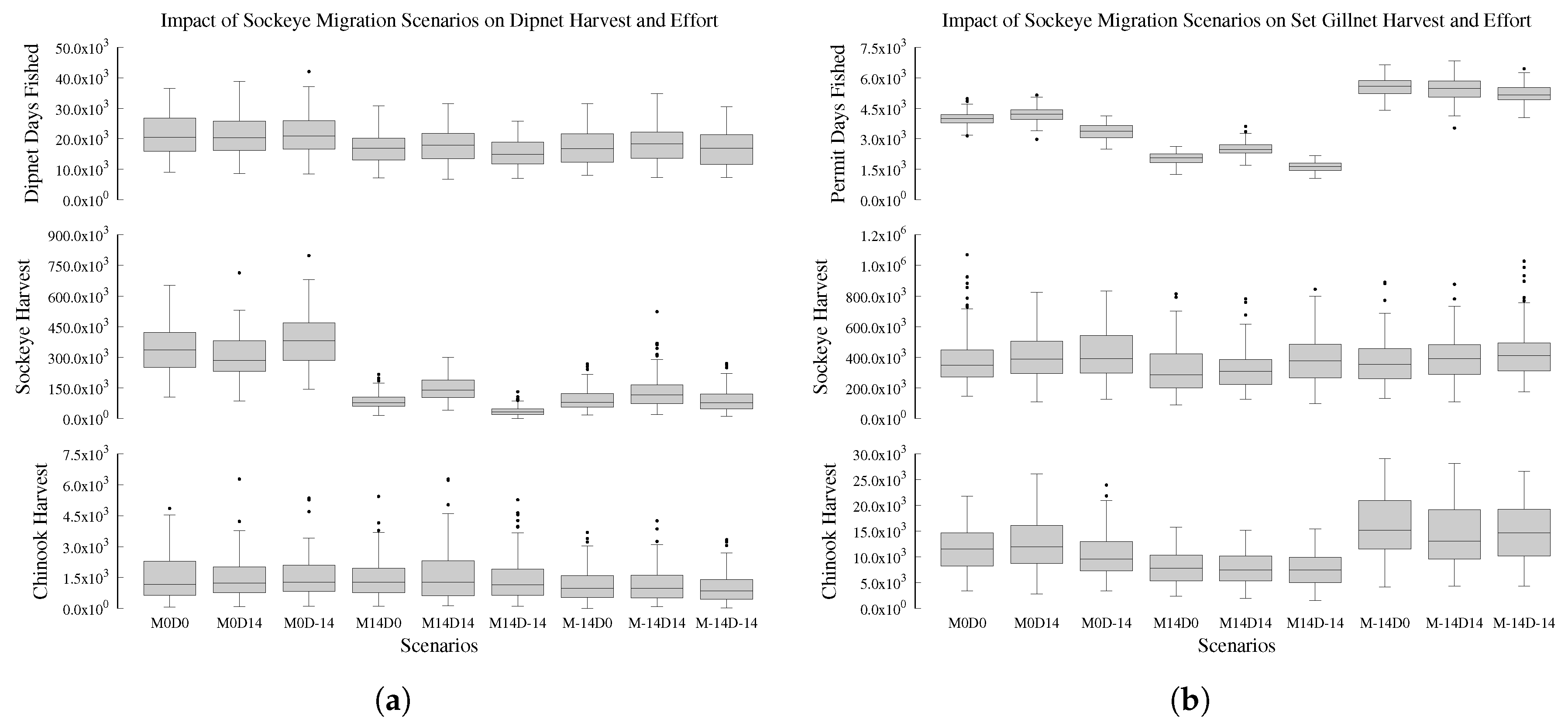
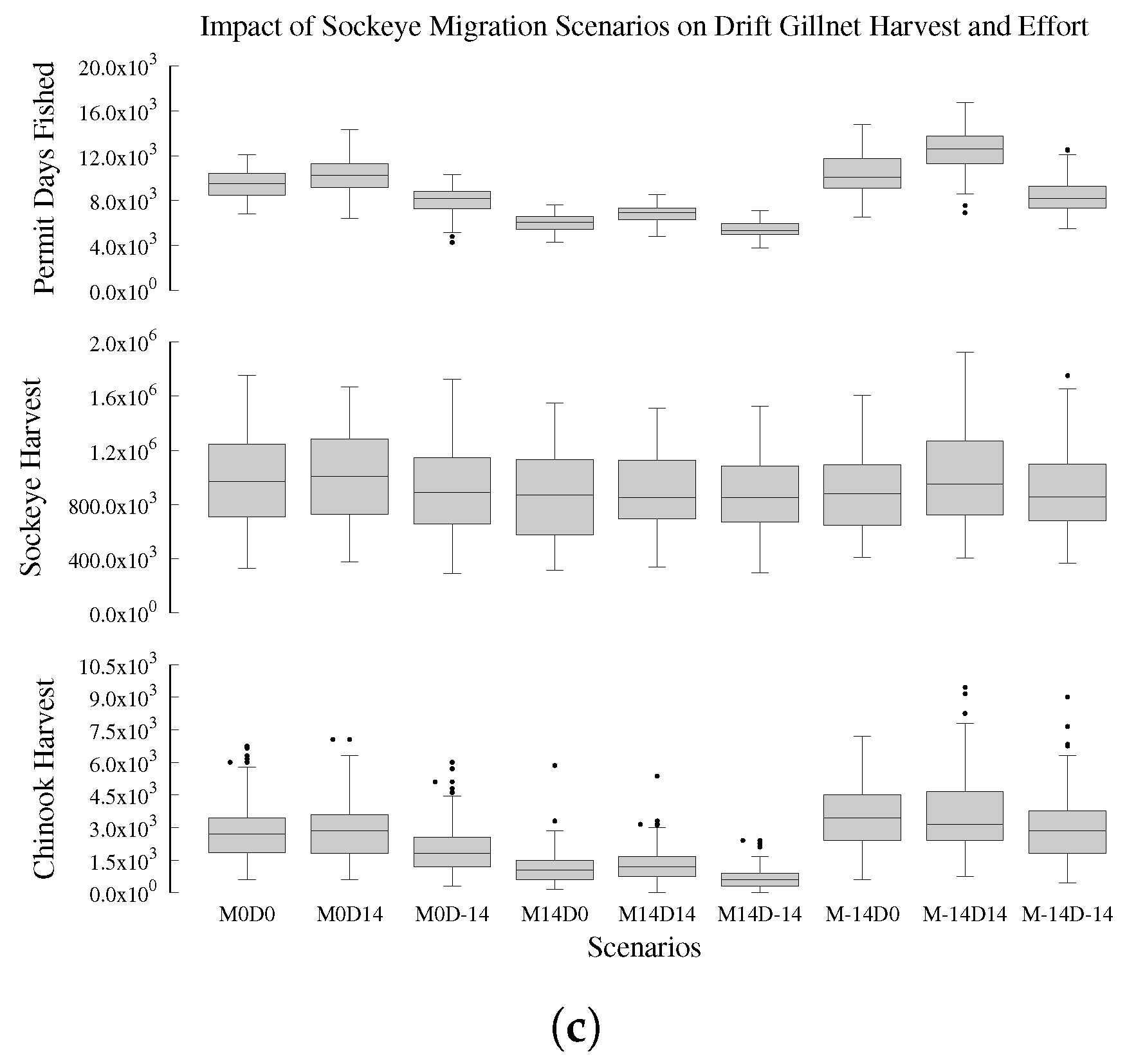
3.1. Sockeye Migration Scenarios

Altering sockeye MDMT and DMT resulted in significant differences in stakeholder harvest and effort (Figure 3a. middle and top panes respectively). The dipnet fishery sockeye harvest was reduced by 54 . 3 % from approximately 185,703–340,778, regardless if the MDMT increased or decreased compared to the control (all scenarios with MDMT = −14 or MDMT = 14 had a p-value < 0.000001 when compared with the M0D0 scenario). These decreases correspond to a $1,130,931–$2,075,332 loss in ex-vessel revenue. Scenario permutations with increased DMT mitigated the effect of altering MDMT. This reflects the critical timing of the short dipnet fishing season from 10 July–31 July to harvest salmon. The high level of effort in the dipnet fishery could be leveraged by policy extending duration of the dipnet fishing season, or setting the dipnet fishing season opening to coincide with observed MDMT changes to sockeye runs.
Figure 3b,c show the commercial set and drift gillnet fisheries harvest (middle panes) with similar trends of reduced effort for scenarios with a later MDMT (top panes). All set gillnet and drift gillnet effort responses showed significant differences with the response for the M0D0 scenario (p-value < 0.000001, with the exception of M0D14 for drift gillnet effort, where p-value = 0.0000024). Unlike the dipnet harvest, the commercial sockeye harvest did not have significant variations. The results of scenarios shifting MDMT later show the current management and commercial fisheries dynamics to be well adapted to shifting migration distribution when fishing occurs later in the season. A beneficial side effect is the reduction of Chinook by-catch due to Chinook arriving earlier in the season relative to the later MDMT shifted sockeye run (bottom panes). Scenarios shifting sockeye MDMT earlier may represent the largest potential challenge to managers, as Chinook by-catch increases due to greater concurrence in timing of the two salmon runs.

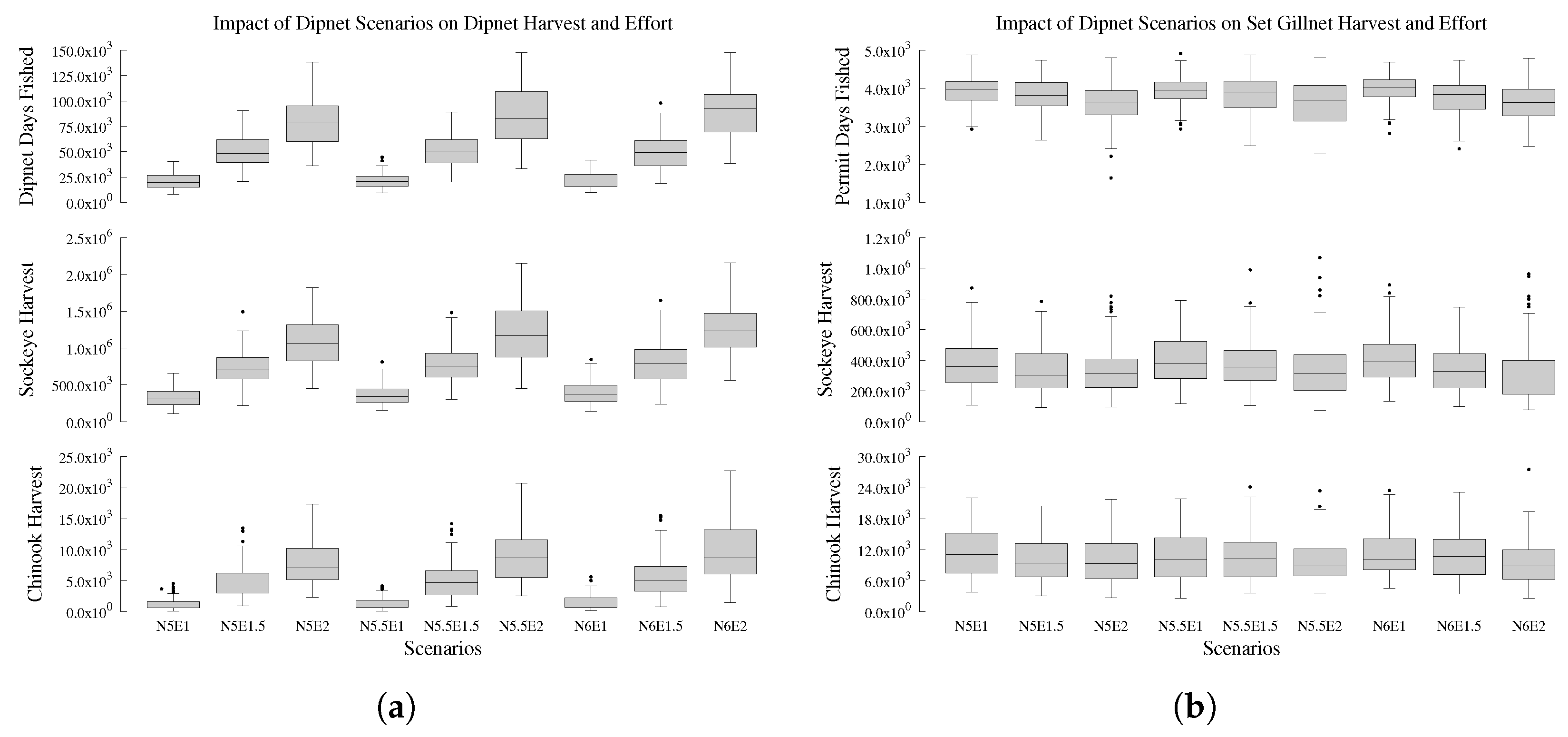
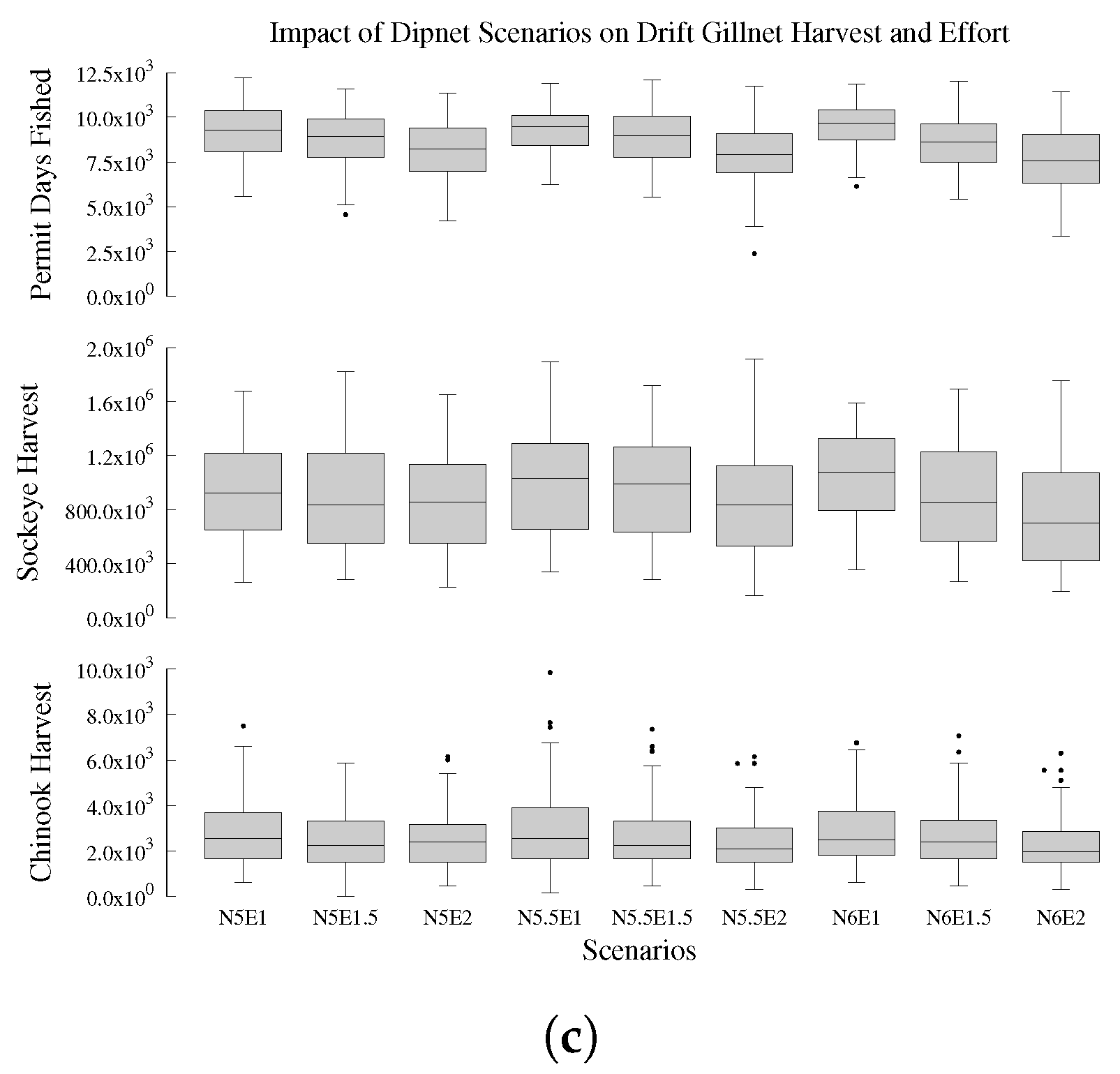
3.2. Dipnet Gear and Effort Scenarios

Gear and effort scenarios altering the number of participating fishermen had a high impact on sockeye and Chinook harvested by dipnetters (Figure 4a). The p-value for all scenarios was < 0 . 000001 when compared with the N5E1 scenario, with the exception of N5.5E1, and N6E1. Therefore, altering dipnet width from 5 ft. to 6 ft. had little to no impact on sockeye and Chinook harvest. As dipnet effort was increased from 1 . 5 2 . 0 times current effort levels, sockeye harvest increased by as much as 346,433–933,835. The corresponding ex-vessel revenue increase ranged from $2,109,777–$5,687,055, completely overtaking in magnitude the ex-vessel revenue lost in the dipnet fishery under the different sockeye salmon migration scenarios.
Figure 4b,c show an unexpected trend of reduced commercial fisheries effort and harvest when dipnet effort and consequently harvest is increased (Tukey HSD: N5E1-N5E2, p-value < 0.000001; N5.5E1-N5.5E2, p-value < 0.000001; N6E1-N6E2, p-value < 0.000001). Drift gillnet harvest decreased by as much as 125,857, leading to an ex-vessel loss of $766,469. Subtracted from the increase in dipnet ex-vessel value, the net increase for dipnet gear and effort scenarios is still $1,343,308–$4,920,586. The reduction in commercial fisheries effort and harvest suggests that current management practices of commercial fisheries adapt to changing levels of dipnet participation and harvest in order to maintain escapement levels. While accommodating the increased dipnet fishery effort might present logistical difficulties, it offers fishery managers additional tools to control and meet sockeye escapement goals (see Figure A2c). Issuing in-season regulatory fishing restrictions to manage dipnet effort would be similar to the use of emergency orders to regulate (increase or decrease) sockeye harvest by commercial fisheries.

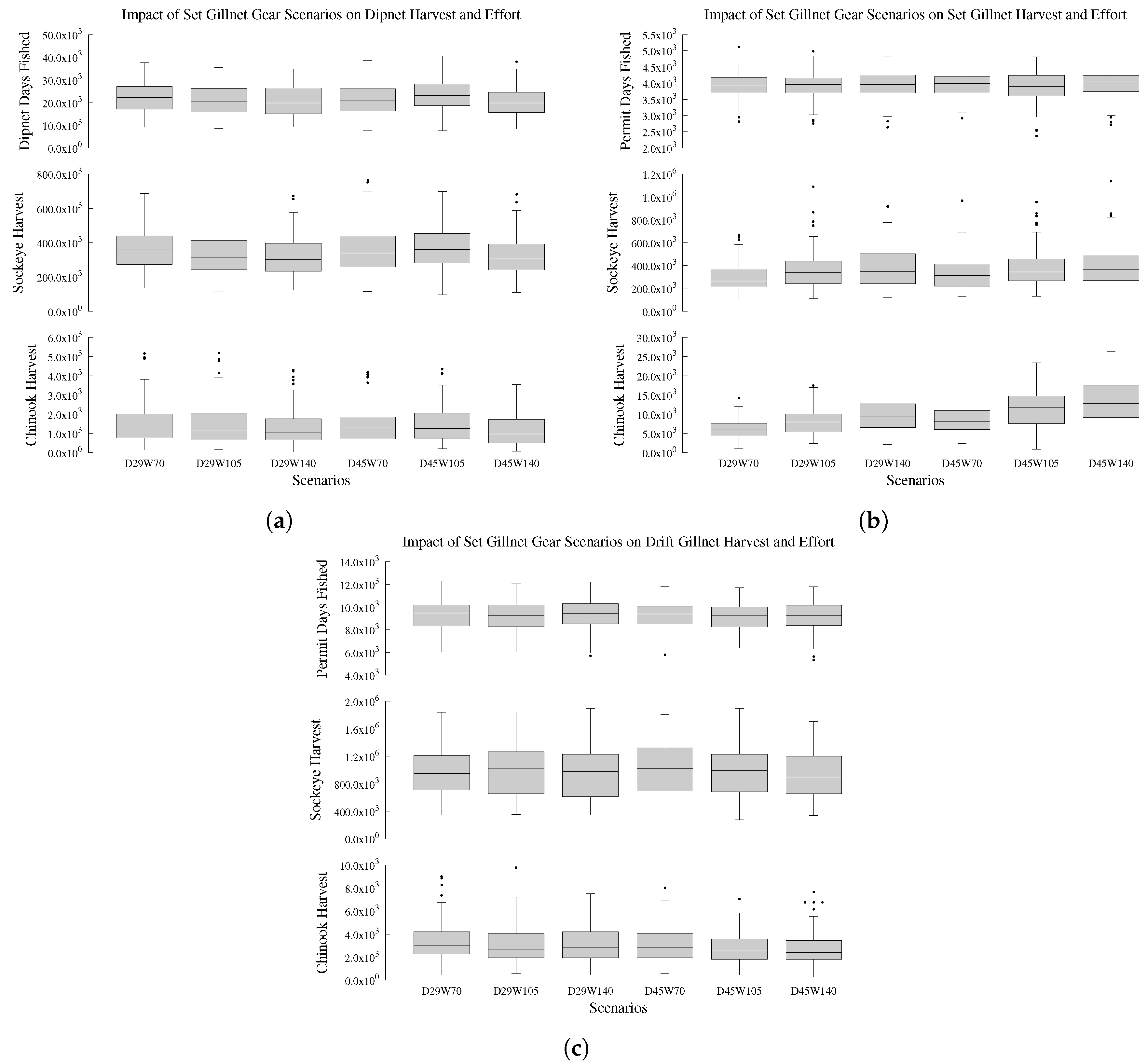
3.3. Set Gillnet Gear Scenarios

Figure 5a shows no significant differences in dipnet response variables of effort and harvest for any of the set gillnet gear scenarios. Also, no significant differences were found for drift gillnet sockeye harvest and effort in all tested scenarios (Figure 5c). A slight decrease in drift gillnet Chinook harvest occurred in scenario D45W140, but was not statistically significant.
Altering the gear also had no significant impacts on set gillnet sockeye harvest (Figure 5b). In contrast to set gillnet sockeye harvest, scenarios D29W70, D29W105, and D45W70 all had significantly reduced Chinook harvest relative to the control (6148–9066, compared with control’s 11,700, p-value < 0.000001), highlighting sensitivity of set gillnet Chinook by-catch to gear alterations.

3.4. Management Implications

The management policy objectives for all Kenai fisheries is a maximum sustainable yield which determines the biological escapement quota which is controlled by the harvest policies that meet all stakeholders’ needs. The significant differences in set gillnet Chinook by-catch support the finding by Welch et al. that Chinook escapement could be increased if set gillnet gear was altered to operate at a depth of 29 meshes and length of 105 fathoms [18]. The steady level of set gillnet effort under different gear alteration scenarios demonstrates how current management strategies may already be efficient at balancing harvest and escapement goals for the set gillnet fishery. Thus, we suggest two important policy implications from this work:
  • Reduction in set gillnet Chinook by-catch, while maintaining sockeye salmon harvest levels, is a critical system dynamic that determines which fisheries are allowed to harvest salmon. If the sockeye run timing dynamics shift earlier, they will coincide with the Chinook runs and as the set gillnet gear scenarios showed, the Chinook by-catch can significantly increase which would shutdown the commercial fisheries closures to protect the Chinook escapement while the dipnet fishery would control the escapement. The alternative management decision would be to limit the set gillnet fishery participation in the early season or regulate the gear dimensions to avoid Chinook by-catch.
  • Increasing dipnet effort and sockeye harvest (Section 3.2) suggests that the dipnet fishery could be used as a sockeye escapement tool and would be especially helpful in years where Chinook escapement is low. The set gillnet fishery would be restricted to minimize the Chinook by-catch while the dipnet fishery harvest would be increased through increased participation. One way of achieving this would be to open the dipnet fishery season to correlate with and knock down the high volume peaks of the sockeye migration dynamics.

4. Conclusions

We presented the first evaluation of alternative fishery policies for the Kenai River watershed in Alaska, utilizing stakeholder-identified socio-ecological drivers and an ABM. The ABM simulates fishery outcomes based on a suite of proposed policy alterations and thus serves as a useful decisions support tool for managers in the region.
This study illustrates an application of a “full circle” conceptual framework to inform fishery management starting from identification of key drivers by stakeholders, formulation of alternative future scenarios, driver sensitivity study using an ABM decision support tool, and a qualitative analysis of alternative policy trade-offs. Analysis of the scenario-based experiments quantified the sensitivity of key socio-ecological drivers on the system’s effort, harvest, and by-catch response. Our findings suggest that the fixed timing of the dipnet fishery limits its ability to respond to altered sockeye migration dynamics, so one potential policy recommendation is to restructure the dipnet fishery season in order to better respond to shifting sockeye migration dynamics. Despite this limitation in the dipnet fishery, we found strong evidence that ADFG currently shows high adaptive capacity in managing and maximizing sockeye harvest in the commercial fisheries under current Chinook and sockeye escapement goals.
Particularly noteworthy was our finding that the commercial fisheries were able to adapt to increased dipnet effort and resulting sockeye harvest which confirms the overall system stability. This conclusion is evident from the scenarios with the increased dipnet effort and sockeye harvest, and the commercial fisheries’ ability to adapted to the changing dipnet dynamics while remaining their sockeye harvest at the same levels.
We also highlight the potential utility of the dipnet fishery as an active management strategy to control sockeye escapement, under increasing dipnet effort scenarios. Although this fishery is not currently used as an active sockeye escapement management tool, the scenarios showed that the dipnet fishery’s increased effort and increased harvest resulted in an increased number of commercial fisheries emergency closures and subsequent decrease in commercial fisheries effort and harvest. The counter-intuitive effect of the downstream dipnet fishery on the commercial fisheries might reduce the emphasis on using the commercial fisheries as the primary escapement management tool. Finally, we find evidence, in a systems-perspective, that adjusting net depth does result in reduced Chinook by-catch by set gillnet fisheries.
Global implications of this work include the utility of integrated ABM modeling as a tool to identify and study the key socio-ecological drivers, test the possible outcomes of the proposed policy change before it is implemented, and assess the adaptive capacity of the fisheries management to absorb rapid and often unexpected system changes. The importance of using integrated ABM modeling to augment the reactionary, practice-based fishery management is likely to increase as the reliability on the historical records becomes increasingly unpredictable due to emergence of never seen system dynamics.

Author Contributions

Authors M.F. and M.C. contributed equally to all aspects of this research project. E.J.T. contributed to stakeholder engagemnt workshops and assessment, identification of key drivers and the conceptualization of the alternative future scenarios.

Funding

This research was funded by Alaska EPSCoR NSF award #OIA-1208927.

Acknowledgments

The authors would like to thank all project collaborators, especially to Dan Rinella, Molly McCarthy, and all participants of the Salmon 2050: Drivers of Change workshop for their input.

Conflicts of Interest

The authors declare no conflict of interest.

Appendix A.

Appendix A.1. Scenario ANOVA p-Values

Table A1. One-Way ANOVA analysis was used for each major scenario grouping to determine if differences were present in the mean of the response variables.
Sockeye, Dipnet, and Set Gillnet Scenario One-Way ANOVA Analysis
Response VariableSockeye p-ValueDipnet p-ValueSet Gillnet p-Value
Dipnet Sockeye Harvest<0.000001<0.0000010.00428
Dipnet Chinook Harvest<0.000001<0.0000010.0885
Dipnet Effort<0.000001<0.0000010.038
Set Gillnet Sockeye Harvest<0.0000010.000028<0.000001
Set Gillnet Chinook Harvest<0.0000010.000706<0.000001
Set Gillnet Effort<0.000001<0.000001<0.000001
Drift Gillnet Sockeye Harvest0.0000926<0.0000010.629
Drift Gillnet Chinook Harvest<0.0000010.0003330.00453
Drift Gillnet Effort<0.000001<0.0000010.89
Sockeye Escapement<0.000001<0.0000010.263
Chinook Escapement<0.000001<0.0000010.0153

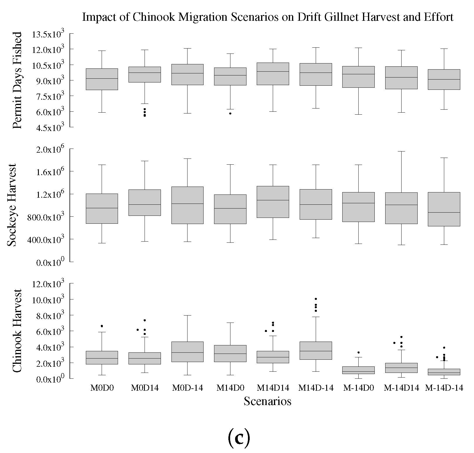
Appendix A.2. Chinook Migration Scenarios

Figure A1 shows the sensitivity of the response variables for scenarios altering Chinook migration dynamics. The results show little to no impact on dipnet, set gillnet or drift gillnet harvest of sockeye salmon. A declining trend can be seen in dipnet Chinook harvest for all scenarios in comparison to the control M0D0 (Figure A1a, bottom pane), and commercial fishery by-catch was reduced for scenarios with an earlier MDMT (Figure A1b,c, bottom pane, M-14D0 to M-14D-14). Tested in isolation, Chinook migration dynamics alone have little impact on driving socio-ecological dynamics. However, if Chinook and sockeye migration dynamics are altered to occur at the same time, the commercial harvest will see an increased Chinook by-catch that (under current management practices) would cause emergency fishery closures and result in difficulties in maximizing commercial sockeye harvest.
Figure A1. Response variables of effort, sockeye harvest, and Chinook harvest for (a) dipnet, (b) set gillnet and (c) drift gillnet fisheries in Chinook migration scenarios altering MDMT and DMT. Scenarios naming convention is identical to Figure 3.
Fishes 04 00033 g0a1aFishes 04 00033 g0a1b

Appendix A.3. Impact of Scenarios on Salmon Escapement

Figure A2. Response variables of sockeye and Chinook escapement were recorded for all scenarios. Escapement for sockeye migration scenarios is in (a). The x-axis is encoded as M standing for median date of migration timing, D standing for duration of migration timing, and the positive or negative numbers standing for the number of days shifted earlier or later. Data for escapement in Chinook migration scenarios (b) is organized the same as (a). Dipnet scenarios multiplying dipnet width (N, in inches) and effort (E) by a multiple of the control value are in (c). Set gillnet scenarios in (b) show of testing different net depths (D, in 6 inch meshes) and net widths (W, in fathoms).
Fishes 04 00033 g0a2aFishes 04 00033 g0a2b

References

  1. Alaska Department of Fish and Game. 2017. Available online: http://www.adfg.alaska.gov (accessed on 1 February 2017).
  2. Heard, W.R. Alaska salmon enhancement: A successful program for hatchery and wild stocks. In Ecology of Aquaculture Species and Enhancement of Stocks, Proceedings of the Thirtieth U.S.—Japan Meeting on Aquaculture. Sarasota, FL, USA, 3–4 December 2001; UJNR Technical Report No. 30; Mote Marine Laboratory: Sarasota, FL, USA, 2001; p. 149. [Google Scholar]
  3. Sechrist, K.; Rutz, J. The History of Upper Cook Inlet Salmon Fisheries A Century of Salmon. 2014. Available online: http://www.adfg.alaska.gov (accessed on 1 February 2017).
  4. Elison, T.B.; Salomone, P.; Brazil, C.E.; Buck, G.B.; West, F.W.; Jones, M.A.; Sands, T.; Krieg, T.; Lemons, T. 2015 Bristol Bay Area Annual Management Report; Alaska Department of Fish and Game, Division of Sport Fish, Research and Technical Services: Anchorage, AK, USA, 2016. [Google Scholar]
  5. Hilborn, R.; Quinn, T.P.; Schindler, D.E.; Rogers, D.E. Biocomplexity and fisheries sustainability. Proc. Natl. Acad. Sci. USA 2003, 100, 6564–6568. [Google Scholar] [CrossRef] [PubMed] [Green Version]
  6. Shields, P.; Dupuis, A. Upper Cook Inlet Commercial Fisheries Annual Management Report, 2011–2014; Reports No. 2014:15-20, 2013:13-49, 2012:13-21, 2011:12-25; Alaska Department of Fish and Game, Division of Sport Fish Commercial Fisheries, Fishery Management: Anchorage, AK, USA, 2015. [Google Scholar]
  7. Shields, P.; Dupuis, A. Upper Cook Inlet Commercial Fisheries Annual Management Report, 2015; Alaska Department of Fish and Game: Anchorage, AK, USA, 2016. [Google Scholar]
  8. Carroll, A. What Are Escapement Goals. 2005. Available online: http://www.adfg.alaska.gov/ (accessed on 1 February 2017).
  9. Clark, R.; Willette, M.; Fleischman, S.; Eggers, D. Biological and Fishery-Related Aspects of Overescapement in Alaskan Sockeye Salmon Oncorhynchus Nerka. Alaska Department of Fish and Game: Anchorage, AK, USA, 2007. [Google Scholar]
  10. Anthony, K.; Marshall, P.A.; Abdulla, A.; Beeden, R.; Bergh, C.; Black, R.; Eakin, C.M.; Game, E.T.; Gooch, M.; Graham, N.A.; et al. Operationalizing resilience for adaptive coral reef management under global environmental change. Glob. Chang. Biol. 2015, 21, 48–61. [Google Scholar] [CrossRef] [PubMed]
  11. Oteros-Rozas, E.; Martín-López, B.; Daw, T.; Bohensky, E.L.; Butler, J.; Hill, R.; Martin-Ortega, J.; Quinlan, A.; Ravera, F.; Ruiz-Mallén, I.; et al. Participatory scenario planning in place-based social- research: Insights and experiences from 23 case studies. Ecol. Soc. 2015, 20. [Google Scholar] [CrossRef]
  12. Shearer, A.W.; Mouat, D.A.; Bassett, S.D.; Binford, M.W.; Johnson, C.W.; Saarinen, J. A Examining development-related uncertainties for environmental management: Strategic planning scenarios in Southern California. Landsc. Urban Plan. 2006, 77, 359–381. [Google Scholar] [CrossRef]
  13. Krupa, M.B. Who’s who in the Kenai River Fishery SES: A streamlined method for stakeholder identification and investment analysis. Mar. Policy 2016, 71, 194–200. [Google Scholar] [CrossRef]
  14. Trammell, J.; Krupa, M.; Powell, J.; Kitty Farnham, K.; Breest, C.; Brummer, C.; Post, L. Salmon 2050. 2019. Available online: https://www.alaska.edu/epscor/archive/phase-4/southcentral-test-case/salmon-2050/ (accessed on 1 April 2017).
  15. Trammell, E.J.; Krupa, M.; Powell, J.; Kliskey, A. Identifying SES threats to salmon abundance on the Kenai River, Alaska. In Preparation.
  16. Alaska Department of Fish and Game. The Kenai River; Technical Report; Alaska Department of Fish and Game: Anchorage, AK, USA.
  17. Shields, P.; Dupuis, A. Upper Cook Inlet Commercial Fisheries Annual Management Report, 2012; Technical Report; Alaska Department of Fish and Game: Anchorage, AK, USA, 2013. [Google Scholar]
  18. Welch, D.W.; Porter, A.D.; Winchell, P. Migration behavior of maturing sockeye (Oncorhynchus nerka) and Chinook salmon (O. tshawytscha) in Cook Inlet, Alaska, and implications for management. Anim. Biotelem. 2014, 2, 35. [Google Scholar] [CrossRef]
  19. Woodby, D.; Carlile, D.; Siddeek, S.; Funk, F.; Clark, J.H.; Hulbert, L. Commercial fisheries of Alaska; Special Publication; Alaska Department of Fish and Game: Anchorage, AK, USA, 2005; p. 74. [Google Scholar]
  20. Dunker, K.J. Upper Cook Inlet Personal Use Salmon Fisheries, 2010–2012; Alaska Department of Fish and Game, Division of Sport Fish, Research and Technical Services: Anchorage, AK, USA, 2013. [Google Scholar]
  21. Kovach, R.P.; Ellison, S.C.; Pyare, S.; Tallmon, D.A. Temporal patterns in adult salmon migration timing across southeast Alaska. Glob. Chang. Biol. 2015, 21, 1821–1833. [Google Scholar] [CrossRef] [PubMed]
  22. Schindler, D.E.; Hilborn, R.; Chasco, B.; Boatright, C.P.; Quinn, T.P.; Rogers, L.A.; Webster, M.S. Population diversity and the portfolio effect in an exploited species. Nature 2010, 465, 609–612. [Google Scholar] [CrossRef] [PubMed]
  23. Taylor, S.G. Climate warming causes phenological shift in Pink Salmon, Oncorhynchus gorbuscha, behavior at Auke Creek, Alaska. Glob. Chang. Biol. 2008, 14, 229–235. [Google Scholar] [CrossRef]
  24. Barclay, A.W.; Habicht, C.; Tobias, T.; Willette, T.M.; Templin, W.D.; Hoyt, H.A.; Chenoweth, E.L. Genetic Stock Identification of Upper Cook Inlet Sockeye Salmon Harvest, 2005–2008, 2009, 2010, 2011; Alaska Department of Fish and Game, Division of Sport Fish, Research and Technical Services: Anchorage, AK, USA, 2010, 2013, 2014. [Google Scholar]
  25. Jones, M.C.; Dye, S.R.; Pinnegar, J.K.; Warren, R.; Cheung, W.W.L. Using scenarios to project the changing profitability of fisheries under climate change. Fish Fish. 2015, 16, 603–622. [Google Scholar] [CrossRef]
  26. Petihakis, G.; Smith, C.J.; Triantafyllou, G.; Sourlantzis, G.; Papadopoulou, K.N.; Pollani, A.; Korres, G. Scenario testing of fisheries management strategies using a high resolution ERSEM–POM ecosystem model. ICES J. Mar. Sci. 2007, 64, 1627. [Google Scholar] [CrossRef]
  27. Weatherdon, L.V.; Ota, Y.; Jones, M.C.; Close, D.A.; Cheung, W.W.L. Projected Scenarios for Coastal First Nations’ Fisheries Catch Potential under Climate Change: Management Challenges and Opportunities. PLoS ONE 2016, 11, e0145285. [Google Scholar] [CrossRef] [PubMed]
  28. Cenek, M.; Franklin, M. An adaptable agent-based model for guiding multi-species Pacific salmon fisheries management within a SES framework. Ecol. Model. 2017, 360, 132–149. [Google Scholar] [CrossRef]
  29. Cenek, M.; Franklin, M. Developing High Fidelity, Data Driven, Verified Agent Based Models Coupled Socio-Ecological Systems of Alaska Fisheries. In Agent-Based Models and Complexity Science in the Age of Geospatial Big Data; Advances in Geographic Information Science; Springer: Cham, Switzerland, 2016. [Google Scholar]
  30. Cenek, M.; Franklin, M. Salmon ABM. 2017. Available online: https://salmonabm.wordpress.com/ (accessed on 1 February 2017).
  31. Cook Inlet Area Commercial Salmon Fishing Regulations 2014–2017. 2013. Available online: http://www.adfg.alaska.gov/ (accessed on 1 February 2017).
  32. Secchi, D.; Seri, R. Controlling for false negatives in agent-based models: A review of power analysis in organizational research. Comput. Math. Organ. Theory 2017, 23, 94–121. [Google Scholar] [CrossRef]
  33. Dowdy, S.; Wearden, S.; Chilko, D. Statistics for Research; John Wiley & Sons: Hoboken, NJ, USA, 2011; Volume 512. [Google Scholar]
  34. Shields, P.; Dupuis, A. Upper Cook Inlet Commercial Fisheries Annual Management Report, 2016; Report No. 2016:17-05 Soldotna; Alaska Department of Fish and Game, Division of Sport Fish and Commercial Fisheries, Fishery Management: Anchorage, AK, USA, 2017. [Google Scholar]
Figure 1. A representative watershed background is generated for each simulation instance. The fishing zones define spatial and temporal areas of the simulation for the stakeholder agents to harvest salmon agents. The fishing zones are defined based on the simulation scale and the pre-season permitting regulations and can be easily altered to represent a policy change. Adapted from [29,30].
Fishes 04 00033 g001
Figure 2. Seasonal distributions of returning salmon agents generated by the ABM from generalized patterns of historical runs. Illustration of the migration-timing scenarios construction for (a) shortening and lengthening DMT shift and (b) shifting the median date of migration distribution.
Fishes 04 00033 g002
Figure 3. Response variables of effort, sockeye harvest, and Chinook harvest for (a) dipnet, (b) set gillnet and (c) drift gillnet fisheries in sockeye migration scenarios altering MDMT and DMT. The x-axis denotes individual scenarios, where M = MDMT shift, numeral = number of MDMT shifted days, D = DMT shift, numeral = number of DMT shifted days. Negative values indicates an earlier shift while positive values are later shifts. Example: M0D14 indicates no shift in MDMT and a DMT shifted 14 days later. Box plots describe: dots on the box plots represent outliers. The middle line of the boxes represents the median, the lower and upper box bounds represent the first and third quartile datapoints respectively. The distance between the first and third quartile is the inter quartile range (IQR). Whiskers represent minimum and maximum values, unless outliers are present, in which case they are taken to be 1.5 × IQR in the direction of the outliers. Unless stated otherwise, the box plot in every sub-plot’s first column is the control.
Fishes 04 00033 g003aFishes 04 00033 g003b
Figure 4. Response variables of effort, sockeye harvest, and Chinook harvest for (a) dipnet, (b) set gillnet and (c) drift gillnet fisheries in dipnet scenarios altering gear and effort. The x-axis denotes individual scenarios, with the following naming convention: N = net width, numeral = net width increase (in feet), E = effort, numeral = effort level relative to the control.
Fishes 04 00033 g004aFishes 04 00033 g004b
Figure 5. Response variables of effort, sockeye harvest, and Chinook harvest for all fisheries for set gillnet gear scenarios altering net depth and width. The x-axis denotes individual scenarios, with following naming convention: D = net depth, numeral = net depth alteration (in meshes), W = net width, numeral = net width alteration (in fathoms). Scenario D45W105 is the control scenario.
Fishes 04 00033 g005
Table 1. A subset of the ABM parameters used in the construction of the scenarios or measured as the model outcomes. The parameter’s default value is the model’s original (verified ground-truth) value, while the ( * ) parameters have their values altered to define a scenario study.
Key Simulation Parameters
ParameterDescriptionDefault Value
Sockeye MDMT Shift  * Shift in median date of migration timing for sockeye salmon run0
Sockeye DMT Shift  * Shift in duration of migration timing for sockeye salmon run0
Chinook MDMT Shift  * Shift in median date of migration timing for Chinook salmon run0
Chinook DMT Shift  * Shift in duration of migration timing for Chinook salmon run0
Set Depth  * Depth of netting used by set gillnet fishermen (6 in. per mesh)45
Set Length (Width)  * Length of netting used by set gillnet fishermen (6 ft. per fathom)105
Dipnet Width  * Largest allowable width for dipnet fishing gear (ft.) 5 . 0
Dipnet Effort Adjust  * Adjustment factor to participation in the dipnet fishery 1 . 0
Dipnetters per AgentSimulation scaling of dipnetters per agent. Altered to affect dipnet effort.34–99
Sockeye Run SizeRandomly selected magnitude of sockeye run strength2,533,975–6,199,394
Chinook Run SizeRandomly selected magnitude of Chinook run strength19,353–75,557
Drift PermitsRandomly selected participation in the drift gillnet fishery378–496
Set PermitsRandomly selected participation in the set gillnet fishery315–385
Drift DepthDepth of netting used by drift gillnet fishermen in meshes (6 in. per mesh)45
Drift LengthLength of netting used by drift gillnet fishermen in fathoms (6 ft. per fathom)150
Table 2. Scenarios were simulated varying the salmon migration and stakeholder gear and effort parameters. Parameter values in brackets represent possible permutation values. Negative MDMT values represent shifts towards earlier migration timing and vice versa for positive MDMT values.
ScenariosParameters AlteredPermutation Values of ParametersUnits
Sockeye MigrationSockeye MDMT Shift[−14, 0, 14]Days
Sockeye DMT Shift[−14, 0, 14]Days
Chinook MigrationChinook MDMT Shift[−14, 0, 14]Days
Chinook DMT Shift[−14, 0, 14]Days
Set Gillnet GearSet Gillnet Depth[29, 45]Meshes (6 in. per mesh)
Set Gillnet Width[70, 105, 140]Fathoms (6 ft. per fathom)
Dipnet Gear and EffortDipnet Width[5.0, 5.5, 6.0]Feet
Dipnet Effort Adjust[1.0, 1.5, 2.0]Constant

