Shelf-Life Prediction of Glazed Large Yellow Croaker (Pseudosciaena crocea) during Frozen Storage Based on Arrhenius Model and Long-Short-Term Memory Neural Networks Model

Abstract

In this study, the changes in centrifugal loss, TVB-N, K-value, whiteness and sensory evaluation of glazed large yellow croaker were analyzed at −10, −20, −30 and −40 °C storage. The Arrhenius prediction model and long-short-term memory neural networks (LSTM-NN) prediction model were developed to predict the shelf-life of the glazed large yellow croaker. The results showed that the quality of glazed large yellow croaker gradually decreased with the extension of frozen storage time, and the decrease in quality slowed down at lower temperatures. Both the Arrhenius model and the LSTM-NN prediction model were good tools for predicting the shelf-life of glazed large yellow croaker. However, for the relative error, the prediction accuracy of LSTM-NN (with a mean value of 7.78%) was higher than that of Arrhenius model (with a mean value of 11.90%). Moreover, the LSTM-NN model had a more intelligent, convenient and fast data processing capability, so the new LSTM-NN model provided a better choice for predicting the shelf-life of glazed large yellow croaker.

1. Introduction

As a nutritious and delicious seawater product, large yellow croaker (Pseudosciaena crocea) is widely loved by consumers. The production of farmed large yellow croaker was 225,549 tons in 2019 [1], which is the largest producer of marine farmed fish in China. However, it is also highly susceptible to spoilage [2]. Freezing and frozen storage are usually used to extend preservation time of large yellow croaker [3] because the low temperature can inhibit the growth of microorganisms and certain enzymatic reactions [4,5]. Therefore, freezing is considered one of the most effective methods of fish preservation, which is widely used both onshore and on fishing vessels.

Although freezing can significantly extend the shelf-life of fish, inevitably, cryopreservation can also lead to several undesirable effects, including moisture loss, protein degradation, loss of freshness, and microstructural disorders [6]. To minimize these undesirable effects, one promising method is achieved by the ice glazing [7,8]. Pre-frozen large yellow croaker is immersed in an ice-cold solution for some time, and the solution forms a thin layer of ice on the surface of the fish, which is considered as a protective layer that serves to avoid contact between the fish and air, reduce dry consumption, and reduce temperature fluctuations [9].

Water is usually used as a raw material for ice glazing. In some recent reports, some natural food additives have been shown to be good alternatives. In a study by Tan et al. [8], an ice glaze containing 0.1% sodium polyacrylate (SP) and 0.3% D-sodium erythorbate (DSE) was effective in extending the duration of squid in frozen storage. Shi et al. [10] found that ice glazes made with rosemary extract were more effective in controlling TVB-N and drip loss.

Shelf-life is a very important quality characteristic of a food product and is of great interest [11], defined as the length of time it can be stored without being unacceptable to the consumer. Similar to other general foods, consumers purchase fish foods determined by physical-chemical attributes such as appearance (color, texture) and odor [12]. In addition to this, total volatile base nitrogen (TVB-N) is often used as a marker of protein and amine degradation, is widely used to interpret the freshness of meat [13] and has corresponding national standards to define its limit values. It is well known that changes in fat can also be a good indicator of changes in fish quality [14], TBARS is one of the most important indicators to assess lipid oxidation, which is used to quantify the secondary by-products of polyunsaturated fatty acid degradation. However, there is no relevant standard to define their limiting values. Therefore, fish spoilage cannot be directly determined by reaching a certain threshold through indicators such as FFA and TBARS.

Multiple accelerated shelf-life testing (MASLT) can monitor different characteristics of food, and it is an acceptable method for shelf-life prediction. In recent years, shelf-life prediction of squids [15], gilthead sea bream [6], and dried shrimp [16] have been mostly predicted using MASLT. Therefore, the MASLT methods were chosen to predict the shelf-life of glazed large yellow croaker in our research.

Kinetic models are now being widely used to predict food quality changes, and there are many reports using the Arrhenius model to simulate the prediction of quality changes in fish. Examples include sardine fillets [17], rainbow trout [18], and tuna [6]. The use of the Arrhenius model provides a good prediction of the quality changes of fish products during storage.

In addition, as artificial intelligence has become more modern, artificial neural networks (ANNs) have been used by researchers to explore the prediction of certain properties of the food industry [19]. ANNs are nonlinear mathematical models consisting of a large number of interconnected neurons that identify complex relationships between input and output data through their strong learning capabilities [20]. ANNs can include back propagation neural networks (BP-NN) and long-short-term memory neural networks (LSTM-NN) [21]. However, according to Wang et al. [22], BP-NN has the weak multi-output ability and self-learning ability. LSTM-NN, as a new neural network model, is used in lithium battery lifetime prediction [23], complex chemical process yield prediction [24], protein structure prediction [25], but applying LSTM-NN to aquatic product shelf-life prediction is almost not reported.

To achieve the goal of predicting the shelf-life of glazed large yellow croaker, we compared TVB-N, K values, water retention, color difference, and sensory analysis of ice-glazed large yellow croaker containing 0.1% SP and 0.3% DSE at different storage conditions (−10 °C, −20 °C, −30 °C, and −40 °C) with reference to the solution formulation of Tan et al. [8]. These data were used to fit the Arrhenius model and LSTM-NN model for shelf-life prediction.

2. Materials and Methods

2.1. Sample Preparation

The large yellow croaker with an average weight of 650 g ± 100 g was purchased from the Luchao Port seafood market and kept fresh for rapid transport back to the laboratory. After sudden death with ice, the fish was transferred to a spiral freezer (Yantai Moon Co., Ltd., Yantai, Shandong, China) for freezing at −35 °C with a wind speed of 10 m/s. The temperature of the center of the large yellow croaker was monitored using a temperature collector (2640A, Fluke, Everett, WA, USA), and the freezing end point of the fish body center was selected as −18 °C. A solution containing 0.1% SP and 0.3% DSE was prepared and used as an ice glaze, stored at 4 °C. The pre-frozen large yellow croaker was immersed in the glazing solution for 25 s, maintaining a glazing ratio of approximately 10%. After glazing, samples were packaged in polyethylene bags and randomly divided into four groups (12 strips per group) and stored at −10, −20, −30, and −40 °C, respectively, and experiments were performed every 30 days. An additional batch of samples (12 strips) was prepared, treated in the same way, and preserved at −5 °C for model validation, with experiments performed every 7 days from day 77 onwards. In addition, large yellow croaker samples were thawed in flowing water (20 ± 5 °C) before testing, and the thawing end point was considered when the fish temperature reached 4 °C.

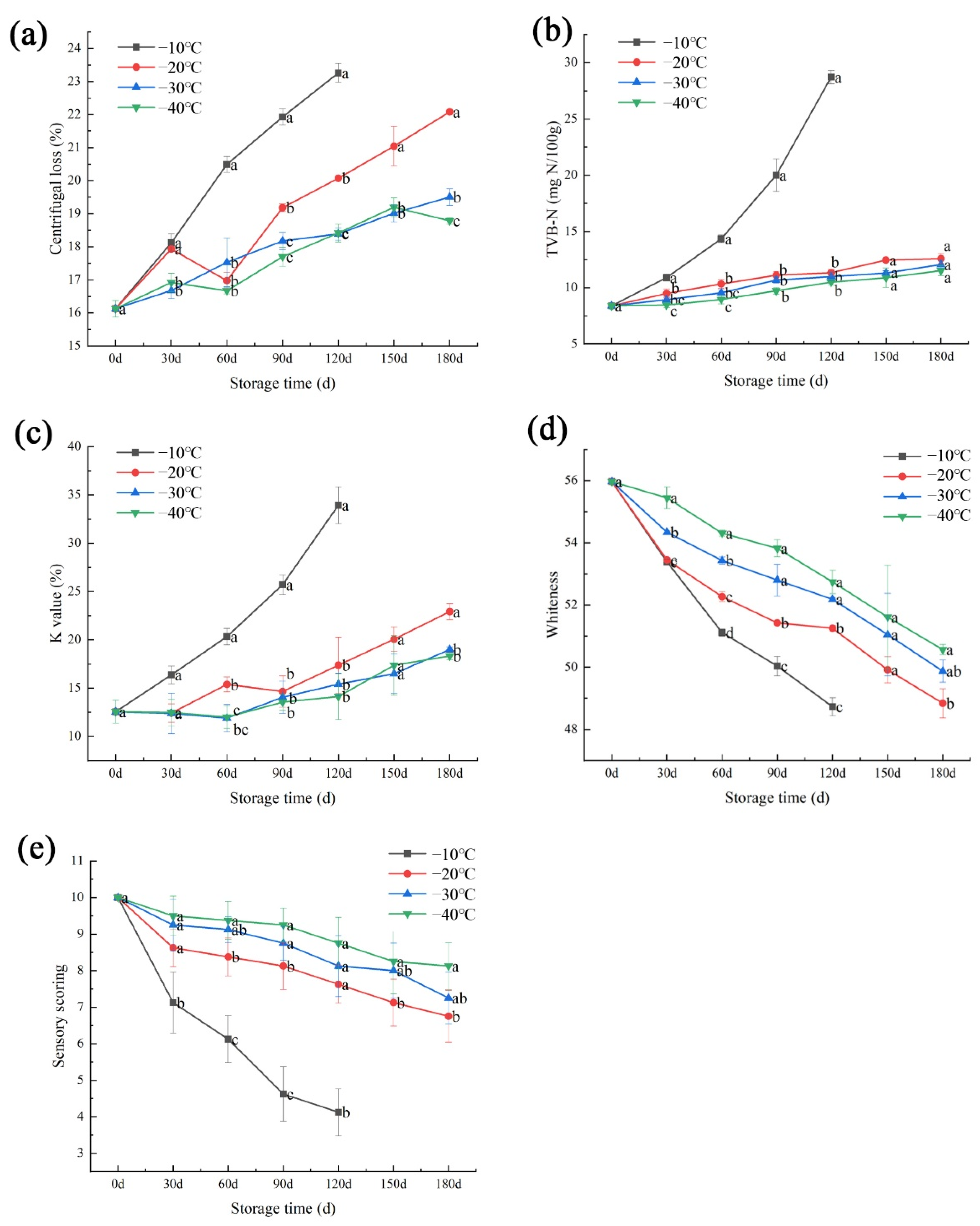
2.2. Centrifugal Loss

Referring to the method of Tan et al. [26], about 2 g of thawed large yellow croaker back muscle was weighed, wrapped in filter paper and loaded into polyethylene centrifuge tubes (50 mL), centrifuged at 5000 r/min for 10 min. Centrifugal loss rate was calculated from the weight before centrifugation (W₁) and the weight after centrifugation (W₂), and each measurement was made in triplicate with the following equation.

$$Centrifugal loss/\%=\left(W_1-W_2\right)W_1\times 100$$

2.3. Total Volatile Base Nitrogen (TVB-N)

Referring to the method of Li et al. [27], five g of chopped large yellow croaker meat was weighed and mixed with 1.5 g of magnesium oxide in a digestion tube. Analyzed using a Kjeldahl nitrogen analyzer (Kjeltec 8400, Foss, Copenhagen, Denmark). The results were expressed as mg N/100 g, and each test was performed in triplicate.

2.4. K Value

ATP-related compounds were improved on the basis of the method of Yang et al. [28]. A 5 g sample was weighed, homogenized by adding 10% v/v perchloric acid solution, centrifuged at 8000 r/min for 15 min at 4 °C, and the supernatant was removed. The supernatant was removed. The precipitate was homogenized again by adding 5% v/v perchloric acid and centrifuged under the same conditions, and this operation was repeated twice. The supernatant was combined and the pH was adjusted to 6.5 with potassium hydroxide solution and placed at 4 °C for 30 min. The supernatant was fixed to 50 mL with ultrapure water and filtered through a 0.22-μm membrane.

The analysis was performed by HPLC (Waters 2695, Milford, CT, USA) using a phosphate buffer at pH 6.5 and methanol in the ratio of 95:5 for 20 min with detection at 254 nm. Each measurement was performed in triplicate.

2.5. Color Measurement

The color of the dorsal muscles of large yellow croaker was measured using a benchtop spectrophotometer (YS6010, Shenzhen Sanenshi Technology Co., Ltd., Shenzhen, China) with a measurement diameter of 8 mm, L*, a*, and b* were used to indicate the brightness, red-green, and yellow-blue color of the muscles, respectively, and each set of samples was repeated five times. The calculation of whiteness was performed according to the following equation.

$$Whiteness=100-\sqrt{{\left(100-L^{*}\right)}^2+a^{*}{}^2+b^{*}{}^2}$$

2.6. Sensory Analysis

The sensory attributes of large yellow croaker were assessed on fish samples by a sensory panel of eight trained evaluators. Based on the method protocol developed by Ozogul et al. [29] with some modifications. The samples were evaluated for the quality of the ice glaze before thawing, and color, odor, tissue morphology, muscle elasticity of the large yellow croaker flesh after thawing. For each parameter, a scale of 1–10 was evaluated (10 being the best quality and 1 being the worst quality).

2.7. Shelf-Life Prediction

To evaluate the shelf-life of ice-glazed large yellow croaker, the Arrhenius model and the LSTM-NN model were used.

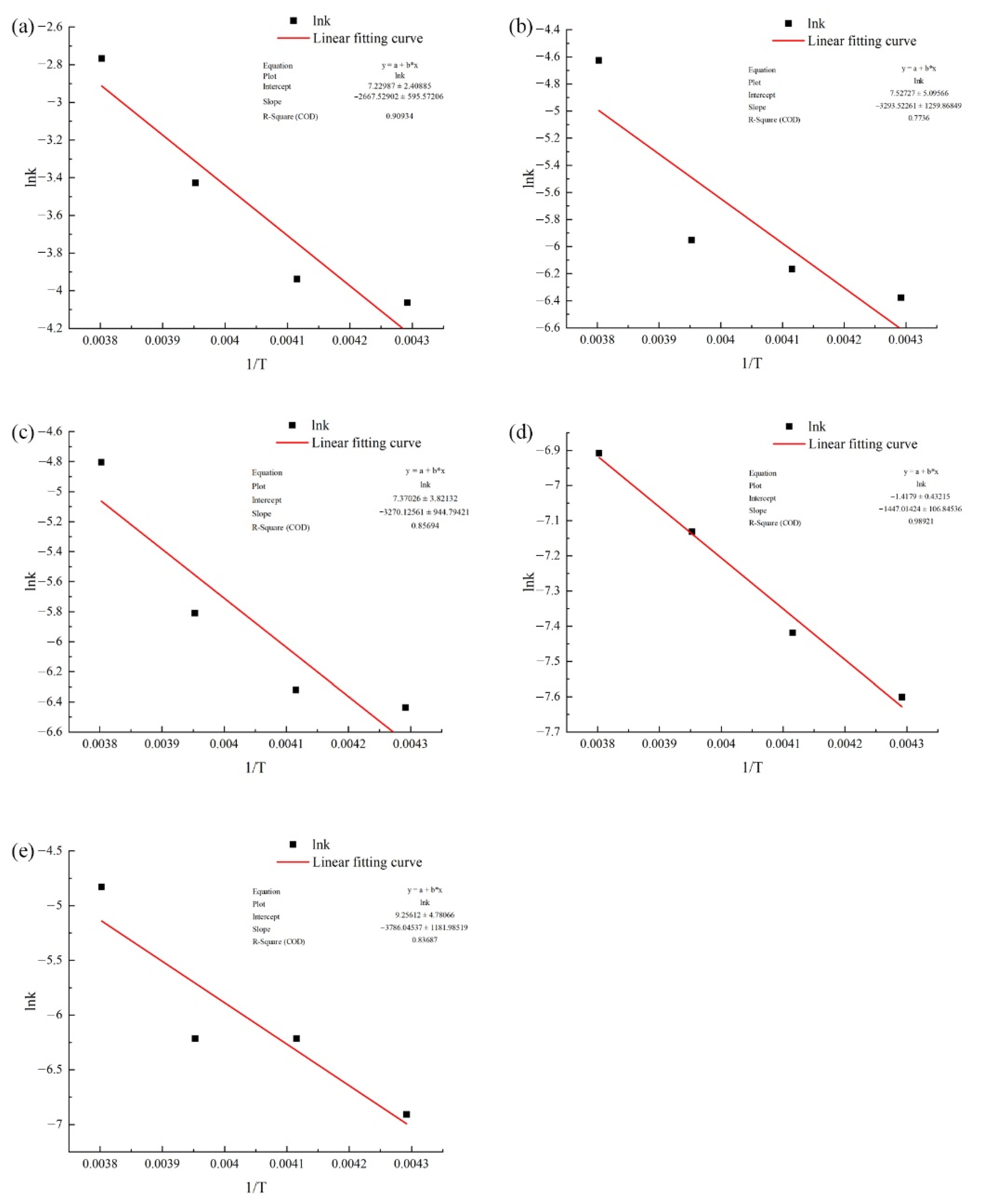
2.7.1. Arrhenius Model

Based on the method of Chaudhry et al. [30]. The shelf-life was assessed by the MASLT method. Firstly, the characteristics that changed significantly with preservation time were selected as indicators of principal component analysis (PCA). Secondly, the time-dependent principal component (PC) was selected as a multivariate kinetic parameter for large yellow croaker shelf-life prediction. The kinetic order, rate constant, activation energy and acceleration factor of the multivariate kinetic parameters were calculated by combining the kinetic equation and Arrhenius equation to predict the shelf-life.

Most foods conform to the zero- or first-order chemical kinetic model, and the reaction rate at a constant temperature according to the mass-action law of the primitive reaction can be expressed in the following metric:

$$V=-\frac{dM}{dt}=k{M}^n$$

where V is the reaction rate; t is the storage time; M is the quality factor; k is the reaction rate constant; and n is the number of reaction stages.

Integrating both sides of the above equation simultaneously yields:

$${{\displaystyle \int }}_{M_0}^M-\frac{dM}{dt}dt={{\displaystyle \int }}_0^{t}k{M}^{n}dt$$

If n = 0, the zero-level dynamics model can be obtained from the above equation:

$$M_0-M=kt$$

If n = 1, the first-level dynamics model can be obtained from the above equation:

$$ln{M}_0-lnM=kt$$

The deformation of the first-order dynamic model can be obtained as follows:

$$M=M_0{e}^{-kt}$$

where M₀ is the initial quality factor.

The reaction rate is significantly dependent on temperature, and if the storage temperature is lower, the quality deterioration of large yellow croaker is slow. Therefore, to correlate or describe the temperature dependence of the quality change, we used the Arrhenius equation, which is a more precise equation describing the relationship between the temperature (T) and the reaction rate constant (k), expressed as follows:

$$k=k_0\exp \left(-\frac{E_a}{RT}\right)$$

where k₀ is the pre-exponential factor; E_a is the activation energy, J/mol; R is the molar gas constant, 8.314 J/(K∙mol); T is the absolute temperature, K.

Combining the kinetic model and the Arrhenius equation, a shelf-life model for ice-glazed large yellow croaker can be developed.

A shelf-life model consistent with zero-level dynamics:

$$SL=\frac{\left|M_0-M\right|}{k_0\exp \left(-\frac{E_a}{RT}\right)}$$

A shelf-life model consistent with first-level dynamics:

$$SL=\frac{\left|ln{M}_0-lnM\right|}{k_0\exp \left(-\frac{E_a}{RT}\right)}$$

where SL is the shelf-life.

Finally, the feasibility of the shelf-life model was verified using large yellow croaker stored at −5 °C to obtain the predicted value X₁ and the measured value X₀, respectively. The following method was used for evaluation:

Relative Error:

$$\mathit{RT}=\frac{X_1-X_0}{X_0}\times 100\%$$

2.7.2. LSTM-NN Model

The LSTM-NN consists of an input layer, one or more implicit layers and an output layer, and uses memory cells to store knowledge, the LSTM-NN model structure is shown by Figure 1. An LSTM block mainly contains memory cell states, forgetting gates, input gates and output gates, where memory cell states are the key elements throughout the LSTM block. Also, with the help of these three gates, certain information can be added and removed selectively [31]. In the figure, x is the input, h is the hidden state that can be given the ability to remember, and t is the storage time. W is the input weights, U is the recurrent weights, and the activation functions σ and tanh are the sigmoid function between 0 and 1 and hyperbolic tangent function, respectively, both of which have the effect of enhancing the nonlinearity of the artificial neural network.

After building the LSTM-NN model, its performance needs to be examined. The prediction correlation coefficient R², root mean square error (RMSE), relative error (RE) and mean absolute percentage error (MAPE) between the predicted and measured values were compared. The formulas are as follows:

$$R^2=1-\frac{{{\displaystyle \sum }}_{i=1}^n{\left(M_i-P_i\right)}^2}{{{\displaystyle \sum }}_{i=1}^n{\left(M_i-\overline{M}\right)}^2}$$

$$RMSE=\sqrt{\frac{1}{n}{\displaystyle \sum }_{i=1}^n{(M_i-P_i)}^2}$$

$$MAPE=\left(\frac{{{\displaystyle \sum }}_{i=1}^n\left|M_i-P_i\right|}{n{M}_i}\right)$$

3. Results

The quality changes under different frozen storage temperatures are shown in Figure 2.

Water holding capacity (WHC) is one of the important characteristics reflecting the quality of fish, which can be reflected by centrifugal loss. The changes of centrifugal loss with storage time at different temperatures is shown in Figure 2a. The initial centrifugal loss was 16.13% and increased significantly with storage time. After 90 days, the centrifugal loss of large yellow croaker stored at −10 °C had reached 21.93% which was 5.80% higher than the initial level, and after 180 days of storage, the centrifugal loss of large yellow croaker stored at −20 °C, −30 °C and −40 °C increased by 5.95%, 3.38%, and 2.65%, respectively. This may be that the higher the storage temperature of the large yellow croaker, the more likely oxidation reaction of fat and protein occur, which results in higher centrifugal loss as they are unable to hydrate with the back-percolating water [32].

The freshness of fish is critical to its consumer acceptance and total volatile base nitrogen (TVB-N) is widely used in determining the freshness of fish products [33]. TVB-N is commonly used as a biomarker for protein and amine degradation and increases with storage time. The National Standard of the People’s Republic of China (PRC) (SC/T 3101-2010) always stipulates that the acceptable range of TVB-N value for large yellow croaker is below 30 mg N/100 g, and its value below 13 mg N/100 g is considered as first grade. The variation of TVB-N value with time at different storage temperatures is shown in Figure 2b. The initial TVB-N value was 8.39 mg N/100 g, which increased during storage. After 120 days of storage at −10 °C, large yellow croaker had a TVB-N value of 28.72, which was close to spoilage. While at the other three storage temperatures (−20 °C, −30 °C, and −40 °C), large yellow croaker remained in the first grade. The possible reason is that the enzymatic activity of protein-degrading enzymes decreases under low temperature and the protein degradation reaction is slow, thus maintaining a lower TVB-N value.

K value is closely related to the degradation of adenosine triphosphate (ATP) and has been widely used for the evaluation of fish freshness [27]. K value below 20% is considered as fresh state and the variation of K value with time is shown in Figure 2c. The initial K value was 12.56%, and there was an increasing trend of K value at all temperatures during the storage period. Among the large yellow croaker stored at −10 °C, the K value increased at the fastest rate, reaching 20.34% after 60 d of storage, which was not a very fresh state. After 180 d of storage at the other three temperatures (−20 °C, −30 °C, and −40 °C), it was still in a very fresh state with K values of 22.92%, 18.99%, and 18.33%, respectively. This is due to the fact that degradation of ATP can be slowed down more effectively under low temperature [34].

The surface color of the samples is a direct basis for consumers to determine whether the fish is fresh or not [35]. All frozen large yellow croaker were measured for whiteness and the results are displayed in Figure 2d. The initial whiteness value of large yellow croaker was 55.97, and the whiteness decreased gradually with increasing storage time during freezing, and the lower the storage temperature, the slower the whiteness value decreased. This is because the low temperature has less effect on protein and fat, and fat oxidation, protein denaturation and pigment degradation can be inhibited to a great extent.

Sensory scores were assessed by a sensory panel of eight evaluators, and sensory scores decreased with frozen storage time and temperature, as illustrated in Figure 2e. According to the panelists’ descriptions, the main influence on the overall acceptability of the samples was the odor of the fish. The large yellow croaker stored at −10 °C for 120 d clearly lost its inherent fresh flavor after thawing. Besides, the color of the fish gradually darkened during storage, especially for samples stored at −10 °C, which was consistent with the results of the analysis of whiteness values.

4. Discussion

4.1. Arrhenius Model

4.1.1. Dynamical Analysis

Based on the centrifugal losses at each storage time at different temperatures, zero-level linear regression analysis and first-level linear regression analysis were performed and fitted to calculate the reaction rate constant, linear regression coefficients of determination, as shown in

Table 1. Kinetic parameters of various indicators of large yellow croaker at different storage temperatures.

	Dynamics Model	Storage Temperature (°C)	Fitting Formula	Reaction Rate Constant	Determination Coefficient R2	∑R2	Ea (kJ/mol)	k0
Centrifugal loss (%)	Zero-level dynamics model	−10	y = 0.0629x + 16.13	0.0629	0.9863	3.8034	22.18	e7.23
		−20	y = 0.0325x + 16.13	0.0325	0.9316
		−30	y = 0.0195x + 16.13	0.0195	0.9843
		−40	y = 0.0172x + 16.13	0.0172	0.9012
	First-level dynamics model	−10	y = 16.13 exp(3.3 × 10−3 x)	0.0033	0.9707	3.7822
		−20	y = 16.13 exp(1.8 × 10−3 x)	0.0018	0.9353
		−30	y = 16.13 exp(1.1 × 10−3 x)	0.0011	0.9786
		−40	y = 16.13 exp(10−3 x)	0.001	0.8976
TVB-N (mg N/100 g)	Zero-level dynamics model	−10	y = 0.1451x + 8.39	0.1451	0.9404	3.8618
		−20	y = 0.0258x + 8.39	0.0258	0.9677
		−30	y = 0.0208x + 8.39	0.0208	0.9775
		−40	y = 0.0165x + 8.39	0.0165	0.9762
	First-level dynamics model	−10	y = 8.39 exp(9.8 × 10−3 x)	0.0098	0.9941	3.8885	27.38	e7.53
		−20	y = 8.39 exp(2.6 × 10−3 x)	0.0026	0.9462
		−30	y = 8.39 exp(2.1 × 10−3 x)	0.0021	0.967
		−40	y = 8.39 exp(1.7 × 10−3 x)	0.0017	0.9812
K value (%)	Zero-level dynamics model	−10	y = 0.1604x + 12.56	0.1604	0.9706	3.5441
		−20	y = 0.0479x + 12.56	0.0479	0.9127
		−30	y = 0.0266x + 12.56	0.0266	0.8558
		−40	y = 0.0244x + 12.56	0.0244	0.805
	First-level dynamics model	−10	y = 12.56 exp(8.2 × 10−3 x)	0.0082	0.998	3.6562	27.19	e7.37
		−20	y = 12.56 exp(3 × 10−3 x)	0.003	0.942
		−30	y = 12.56 exp(1.8 × 10−3 x)	0.0018	0.8829
		−40	y = 12.56 exp(1.6 × 10−3 x)	0.0016	0.8333
Whiteness	Zero-level dynamics model	−10	y = −0.0656x + 55.97	0.0656	0.9663	3.8751
		−20	y = −0.0423x + 55.97	0.0423	0.939
		−30	y = −0.0339x + 55.97	0.0339	0.9813
		−40	y = −0.0284x + 55.97	0.0248	0.9885
	First-level dynamics model	−10	y = 55.97 exp(−10−3 x)	0.001	0.9734	3.8859	12.03	e−1.42
		−20	y = 55.97 exp(−8 × 10−4 x)	0.0008	0.9446
		−30	y = 55.97 exp(−6 × 10−4 x)	0.0006	0.9819
		−40	y = 55.97 exp(−5 × 10−4 x)	0.0005	0.986
Sensory analysis	Zero-level dynamics model	−10	y = −0.0558x + 10	0.0558	0.9278	3.799
		−20	y = −0.0196x + 10	0.0196	0.9352
		−30	y = −0.0147x + 10	0.0147	0.9714
		−40	y = −0.0106x + 10	0.0106	0.9646
	First-level dynamics model	−10	y = 10 exp(−8 × 10−3 x)	0.008	0.9765	3.8537	31.48	e9.26
		−20	y = 10 exp(−2 × 10−3 x)	0.002	0.9481
		−30	y = 10 exp(−2 × 10−3 x)	0.002	0.9678
		−40	y = 10 exp(−10−3 x)	0.001	0.9613

. From the table, it can be found that the sum of zero-level linear regression coefficients of determination is greater than that of the first-level linear regression coefficients of determination, so it can be indicated that for the WHC of frozen large yellow croaker, the zero-level kinetic linear regression fitting was more advantageous [36]. The temperature dependence of the increased centrifugal losses is well illustrated by Arrhenius kinetics. The E_a value of 23.094 kJ/mol (R² = 0.9003) was also calculated for the 95% confidence range based on the variation of centrifugal losses, combined with the Arrhenius equation for lnk versus 1/T, and pre-exponential factor k₀ is e^7.69, as shown in Figure 3a.

The TVB-N, K-value, whiteness, and sensory were more advantageously fitted by zero-level linear regression analysis and first-level linear regression analysis using first-level kinetic linear regression (Table 1). Arrhenius kinetics adequately described the temperature dependence of TVB-N, K-value, whiteness, and sensory score changes in fish samples over the temperature range studied, showing 95% confidence range activation energy E_a values of 27.38 kJ/mol (R² = 0.7736), 27.19 kJ/mol (R² = 0.8569), 12.03 kJ/mol (R² = 0.9892), and 31.48 kJ/mol (R² = 0.8369).

The whiteness and sensory of large yellow croaker gradually decreased with the extension of frozen storage, so k was negative, and it was automatically converted to ln (−k) when lnk was taken. According to Figure 3b–e, the pre-exponential factors of TVB-N, K value, whiteness and sensory evaluation in large yellow croaker samples were calculated as e^7.53, e^7.37, e^−1.42, e^9.26 respectively.

4.1.2. Shelf-Life Modeling and Shelf-Life Forecasting

Based on the pre-exponential factor (k₀), the reaction activation energy (E_a) and the number of reaction steps obtained from the kinetic analysis, the equations of the shelf-life model conforming to the number of reaction steps were determined, respectively, as follows:

$$S{L}_{\mathit{centrifugal} \mathit{loss}}=\frac{\left|16.13-M_{\mathit{centrifugal} \mathit{loss}}\right|}{e^{7.69}{e}^{-\frac{23.09\times {10}^3}{8.314T}}}$$

$$S{L}_{\mathit{TVB}-N}=\frac{\left|{\mathit{ln}}_{8.39}-{\mathit{ln}}_{M_{\mathit{TVB}-N}}\right|}{e^{7.53}{e}^{-\frac{27.38\times {10}^3}{8.314T}}}$$

$$S{L}_{K \mathit{value}}=\frac{\left|{\mathit{ln}}_{12.56}-{\mathit{ln}}_{M_{K \mathit{value}}}\right|}{e^{7.37}{e}^{-\frac{27.19\times {10}^3}{8.314T}}}$$

$$S{L}_{\mathit{whiteness}}=\frac{\left|{\mathit{ln}}_{55.97}-{\mathit{ln}}_{M_{\mathit{whiteness}}}\right|}{e^{-1.42}{e}^{-\frac{12.03\times {10}^3}{8.314T}}}$$

$$S{L}_{\mathit{Sensory}}=\frac{\left|{\mathit{ln}}_{10}-{\mathit{ln}}_{M_{\mathit{Sensory}}}\right|}{e^{9.26}{e}^{-\frac{31.48\times {10}^3}{8.314T}}}$$

where M_{centrifugal loss}, M_TVB-N, M_{K value}, M_whiteness, and M_sensory are the endpoint critical values of sample quality indicators.

Preservation of samples at −10 °C for 120 days is generally unacceptable to professional reviewers. So the shelf-life separately using the values of each index stored at −10 °C for 90 days was determined as the threshold values. The estimation results are shown in

Table 2. Comparison of predicted shelf-life and measured shelf-life for each indicator at different storage temperatures.

	Storage Temperature (°C)	Predicted Shelf-Life (d)	Measured Shelf-Life (d)	Relative Error (%)
Centrifugal loss (%)	−5	88	98	−9.56
	−10	107
	−20	160
	−30	246
	−40	394
TVB-N (mg N/100 g)	−5	101	112	−9.61
	−10	128
	−20	210
	−30	358
	−40	641
K value (%)	−5	90	105	−14.28
	−10	114
	−20	186
	−30	316
	−40	563
Whiteness	−5	102	112	−8.49
	−10	114
	−20	141
	−30	179
	−40	231
Sensory analysis	−5	115	98	17.56
	−10	151
	−20	266
	−30	493
	−40	962

. Using the verified values at 5 °C as reference, the predicted shelf-life of centrifugal loss, TVB-N, K value, and whiteness were 88, 101, 90, and 102 days respectively with the actual values (98, 112, 105, and 112 days) within 15% error. In assessing and predicting the freshness of catfish stored at different temperatures, Wang et al. found that the relative error of TVB-N was within 10% for the Arrhenius model [22]. Therefore, it can be shown that the prediction model of shelf-life of large yellow croaker established by Arrhenius kinetic model can better reflect the changes of fish quality.

4.2. LSTM-NN Model

The effects of frozen storage and storage temperature on the quality of large yellow croaker were modeled and calculated with MATLAB. To evaluate the effectiveness of our developed LSTM-NN model based on the predicted storage time of glazed large yellow croaker at different temperatures, data from a total of 26 sample points measured at −10, −20, −30, and −40 °C were disrupted and randomly ordered and used to train the model. The thresholds and weights of the connection parameters between neurons were optimized in order to minimize the RMSE of the predicted and measured values during training [18]. The changes of RMSE and loss are shown in Figure 4a. When training was performed, the model performed 500 iterations in 16 s, the RMSE and loss kept decreasing rapidly and basically stabilized after the 150th cycle, which indicated that the LSTM-NN model can predict the shelf-life time well after several training sessions.

The six sample points (day 77, 84, 91, 98, 105, and 112, respectively) measured at −5 °C were used as a test of model validity, and the measured and predicted values are shown in Figure 4b. To better reflect the error between the measured and predicted values, the relative error was calculated, as shown in Figure 4c. From the figure, it can be found that the relative errors were within 8% for all sample points except for the first sample point which reached 19.05%, which indicated that the accuracy of the model was acceptable. In terms of relative errors, the predictions of the LSTM-NN model were more accurate than those of the Arrhenius model. In addition, MAPE and RMSE values are often used to reflect the difference between the predicted and measured values, and after calculation, the MAPE value was 7.78% and the RSME value was 7.94, both of which could show the high prediction accuracy of the LSTM-NN model.

Tan et al. [15] compared the prediction ability of Back propagation neural network (BP-NN) model and LSTM-NN model, and found that the relative error values of LSTM-NN were all within 7%, MAPE and RMSE were lower compared to BP-NN model; Qing et al. demonstrated that LSTM-NN can effectively improve the prediction of solar irradiation by 42.9% and is more stable compared to BP-NN [37], indicating that LSTM-NN models had higher prediction accuracy and were worth using as a shelf-life prediction tool.

5. Conclusions

In this study, we compared the centrifugal loss, TVB-N, K value, whiteness and sensory evaluation of large yellow croaker during frozen storage at −10, −20, −30 and −40 °C. The results showed that the quality decreased significantly with increasing storage time. At lower storage temperatures of, for example, −30 and −40 °C, the quality of large yellow croaker changed less. After 120 days of storage at −10 °C, large yellow croaker produced unacceptable odor and unacceptable values of other indicators. Based on centrifugal loss, TVB-N, K-value, whiteness and sensory evaluation, an Arrhenius prediction model and LSTM-NN prediction model were designed to predict the shelf-life of ice-glazed large yellow croaker during frozen storage. The modeling results showed that for both predicted and measured values, both models had small relative errors and were reliable models for predicting the shelf-life of frozen large yellow croaker. In terms of relative errors, the predictions of the LSTM-NN model were more accurate than those of the Arrhenius model. In addition, in terms of data processing, the LSTM-NN model is more intelligent and less time-consuming compared with the Arrhenius model. In conclusion, the LSTM-NN model is a good tool for predicting the storage time of large yellow croaker.

References

1. China Statistics Press. China Fishery Statistical Yearbook; China Agricultural Press: Beijing, China, 2020; pp. 22–23. [Google Scholar]
2. Aponte, M.; Anastasio, A.; Marrone, R.; Mercogliano, R.; Peruzy, M.F.; Murru, N. Impact of gaseous ozone coupled to passive refrigeration system to maximize shelf-life and quality of four different fresh fish products. LWT 2018, 93, 412–419. [Google Scholar] [CrossRef]
3. Cartagena, L.; Puértolas, E.; de Marañón, I.M. Application of high pressure processing after freezing (before frozen storage) or before thawing in frozen albacore tuna (Thunnus alalunga). Food Bioprocess Technol. 2020, 13, 1791–1800. [Google Scholar] [CrossRef]
4. Truong, B.Q.; Buckow, R.; Nguyen, M.H.; Stathopoulos, C.E. High pressure processing of barramundi (Lates calcarifer) muscle before freezing: The effects on selected physicochemical properties during frozen storage. J. Food Eng. 2016, 169, 72–78. [Google Scholar] [CrossRef]
5. Zhang, M.; Haili, N.; Chen, Q.; Xia, X.; Kong, B. Influence of ultrasound-assisted immersion freezing on the freezing rate and quality of porcine longissimus muscles. Meat Sci. 2018, 136, 1–8. [Google Scholar] [CrossRef] [PubMed]
6. Tsironi, T.N.; Stoforos, N.G.; Taoukis, P.S. Quality and shelf-life modeling of frozen fish at constant and variable temperature conditions. Foods 2020, 9, 1893. [Google Scholar] [CrossRef] [PubMed]
7. Trigo, M.; Rodríguez, A.; Dovale, G.; Pastén, A.; Vega-Gálvez, A.; Aubourg, S.P. The effect of glazing based on saponin-free quinoa (Chenopodium quinoa) extract on the lipid quality of frozen fatty fish. LWT 2018, 98, 231–236. [Google Scholar] [CrossRef] [Green Version]
8. Tan, M.; Li, P.; Yu, W.; Wang, J.; Xie, J. Effects of glazing with preservatives on the quality changes of squid during frozen storage. Appl. Sci. 2019, 9, 3847. [Google Scholar] [CrossRef] [Green Version]
9. Žoldoš, P.; Popelka, P.; Marcinčák, S.; Nagy, J.; Mesarčová, L.; Pipová, M.; Jevinová, P.; Nagyová, A.; Maľa, P. The effect of glaze on the quality of frozen stored Alaska pollack (Theragra chalcogramma) fillets under stable and unstable conditions. Acta Vet. Brno 2011, 80, 299–304. [Google Scholar] [CrossRef] [Green Version]
10. Shi, J.; Lei, Y.; Shen, H.; Hong, H.; Yu, X.; Zhu, B.; Luo, Y. Effect of glazing and rosemary (Rosmarinus officinalis) extract on preservation of mud shrimp (Solenocera melantho) during frozen storage. Food Chem. 2019, 272, 604–612. [Google Scholar] [CrossRef] [PubMed]
11. Mercogliano, R.; De Felice, A.; Cortesi, M.L.; Murru, N.; Marrone, R.; Anastasio, A. Biogenic amines profile in processed bluefin tuna (Thunnus thynnus) products. CyTA-J. Food 2013, 11, 101–107. [Google Scholar] [CrossRef] [Green Version]
12. Holman, B.W.B.; Kerry, J.P.; Hopkins, D.L. A review of patents for the smart packaging of meat and muscle-based food products. Recent Pat. Food. Nutr. Agric. 2018, 9, 3–13. [Google Scholar] [CrossRef]
13. Bekhit, A.E.-D.A.; Holman, B.W.B.; Giteru, S.G.; Hopkins, D.L. Total volatile basic nitrogen (TVB-N) and its role in meat spoilage: A review. Trends Food Sci. Technol. 2021, 109, 280–302. [Google Scholar] [CrossRef]
14. English, M.M.; Scrosati, P.M.; Aquino, A.J.; McSweeney, M.B.; Gulam Razul, M.S. Novel carbohydrate blend enhances chemical and sensory properties of lobster (Homarus americanus) after one-year frozen storage. Food Res. Int. 2020, 137, 109697. [Google Scholar] [CrossRef] [PubMed]
15. Tan, M.; Wang, J.; Li, P.; Xie, J. Storage time prediction of glazed frozen squids during frozen storage at different temperatures based on neural network. Int. J. Food Prop. 2020, 23, 1663–1677. [Google Scholar] [CrossRef]
16. Li, D.; Xie, H.; Liu, Z.; Li, A.; Li, J.; Liu, B.; Liu, X.; Zhou, D. Shelf life prediction and changes in lipid profiles of dried shrimp (Penaeus vannamei) during accelerated storage. Food Chem. 2019, 297, 124951. [Google Scholar] [CrossRef] [PubMed]
17. Corzo, O.; Bracho, N.; Marjal, J. Color change kinetics of sardine sheets during vacuum pulse osmotic dehydration. J. Food Eng. 2006, 75, 21–26. [Google Scholar] [CrossRef]
18. Liu, X.; Jiang, Y.; Shen, S.; Luo, Y.; Gao, L. Comparison of Arrhenius model and artificial neuronal network for the quality prediction of rainbow trout (Oncorhynchus mykiss) fillets during storage at different temperatures. LWT-Food Sci. Technol. 2015, 60, 142–147. [Google Scholar] [CrossRef]
19. Mohammadi Lalabadi, H.; Sadeghi, M.; Mireei, S.A. Fish freshness categorization from eyes and gills color features using multi-class artificial neural network and support vector machines. Aquac. Eng. 2020, 90, 102076. [Google Scholar] [CrossRef]
20. Marini, F. Artificial neural networks in foodstuff analyses: Trends and perspectives A review. Anal. Chim. Acta 2009, 635, 121–131. [Google Scholar] [CrossRef]
21. Yu, L.; Qu, J.; Gao, F.; Tian, Y. A novel hierarchical algorithm for bearing fault diagnosis based on stacked LSTM. Shock Vib. 2019, 2019, 2756284. [Google Scholar] [CrossRef]
22. Wang, H.; Kong, C.; Li, D.; Qin, N.; Fan, H.; Hong, H.; Luo, Y. Modeling quality changes in brined bream (Megalobrama amblycephala) fillets during storage: Comparison of the Arrhenius model, BP, and RBF neural network. Food Bioprocess Technol. 2015, 8, 2429–2443. [Google Scholar] [CrossRef]
23. Cheng, G.; Wang, X.; He, Y. Remaining useful life and state of health prediction for lithium batteries based on empirical mode decomposition and a long and short memory neural network. Energy 2021, 232, 121022. [Google Scholar] [CrossRef]
24. Han, Y.; Fan, C.; Xu, M.; Geng, Z.; Zhong, Y. Production capacity analysis and energy saving of complex chemical processes using LSTM based on attention mechanism. Appl. Therm. Eng. 2019, 160, 114072. [Google Scholar] [CrossRef]
25. Conover, M.; Staples, M.; Si, D.; Sun, M.; Cao, R. AngularQA: Protein model quality assessment with LSTM networks. Comput. Math. Biophys. 2019, 7, 1–9. [Google Scholar] [CrossRef]
26. Tan, M.; Ye, J.; Chu, Y.; Xie, J. The effects of ice crystal on water properties and protein stability of large yellow croaker (Pseudosciaena crocea). Int. J. Refrig. 2021, 130, 242–252. [Google Scholar] [CrossRef]
27. Li, P.; Chen, Z.; Tan, M.; Mei, J.; Xie, J. Evaluation of weakly acidic electrolyzed water and modified atmosphere packaging on the shelf life and quality of farmed puffer fish (Takifugu obscurus) during cold storage. J. Food Saf. 2020, 40, e12773. [Google Scholar] [CrossRef]
28. Yang, W.; Shi, W.; Zhou, S.; Qu, Y.; Wang, Z. Research on the changes of water-soluble flavor substances in grass carp during steaming. J. Food Biochem. 2019, 43, e12993. [Google Scholar] [CrossRef] [PubMed]
29. Ozogul, Y.; Yuvka, İ.; Ucar, Y.; Durmus, M.; Kösker, A.R.; Öz, M.; Ozogul, F. Evaluation of effects of nanoemulsion based on herb essential oils (rosemary, laurel, thyme and sage) on sensory, chemical and microbiological quality of rainbow trout (Oncorhynchus mykiss) fillets during ice storage. LWT 2017, 75, 677–684. [Google Scholar] [CrossRef]
30. Chaudhry, M.M.A.; Amodio, M.L.; Babellahi, F.; de Chiara, M.L.V.; Amigo Rubio, J.M.; Colelli, G. Hyperspectral imaging and multivariate accelerated shelf life testing (MASLT) approach for determining shelf life of rocket leaves. J. Food Eng. 2018, 238, 122–133. [Google Scholar] [CrossRef]
31. Song, X.; Liu, Y.; Xue, L.; Wang, J.; Zhang, J.; Wang, J.; Jiang, L.; Cheng, Z. Time-series well performance prediction based on Long Short-Term Memory (LSTM) neural network model. J. Pet. Sci. Eng. 2020, 186, 106682. [Google Scholar] [CrossRef]
32. Yin, X.; Luo, Y.; Fan, H.; Wu, H.; Feng, L. Effect of previous frozen storage on quality changes of grass carp (Ctenopharyngodon idellus) fillets during short-term chilled storage. Int. J. Food Sci. Technol. 2014, 49, 1449–1460. [Google Scholar] [CrossRef]
33. Chen, H.-Z.; Zhang, M.; Bhandari, B.; Guo, Z. Evaluation of the freshness of fresh-cut green bell pepper (Capsicum annuum var. grossum) using electronic nose. LWT 2018, 87, 77–84. [Google Scholar] [CrossRef] [Green Version]
34. Li, D.; Qin, N.; Zhang, L.; Li, Q.; Prinyawiwatkul, W.; Luo, Y. Degradation of adenosine triphosphate, water loss and textural changes in frozen common carp (Cyprinus carpio) fillets during storage at different temperatures. Int. J. Refrig. 2019, 98, 294–301. [Google Scholar] [CrossRef]
35. Ji, E.; Woong, H.; Bae, Y.; Hoon, S.; Se, J.; Hyun, H. Effect of tempering methods on quality changes of pork loin frozen by cryogenic immersion. Meat Sci. 2017, 124, 69–76. [Google Scholar] [CrossRef]
36. Lau, M.; Tang, J.; Swanson, B. Kinetics of textural and color changes in green asparagus during thermal treatments. J. Food Eng. 2000, 45, 231–236. [Google Scholar] [CrossRef]
37. Qing, X.; Niu, Y. Hourly day-ahead solar irradiance prediction using weather forecasts by LSTM. Energy 2018, 148, 461–468. [Google Scholar] [CrossRef]
Figure 1. Schematic diagram of LSTM-NN model structure.
Fishes 06 00039 g001
Figure 2. Centrifugal loss (a), TVB-N (b), K value (c), whiteness (d) and sensory scoring (e) of large yellow croaker at different storage temperatures. The means between different frozen storage temperatures on the same days with different lowercase letters (a–d) differ significantly.
Fishes 06 00039 g002
Figure 3. Relationships between the rate of change of centrifugal loss (a), TVB-N (b), K value (c), whiteness (d) and sensory scoring (e) of large yellow croaker at different storage temperatures.
Fishes 06 00039 g003
Figure 4. Training Chengo curve (a), comparison (b) and relative error (c) between predicted and measured values of LSTM-NN model.
Fishes 06 00039 g004