Influence of Spatial Scale Selection of Environmental Factors on the Prediction of Distribution of Coilia nasus in Changjiang River Estuary

Abstract

An estuary region is a complex environment with a transition from fresh to brackish to salt water, and in which some environmental factors change dramatically over small ranges. Therefore, it is important to understand the impact of the selection of spatial scale on the prediction of the distribution of estuarine species. As the largest estuary in China, the Changjiang River estuary is the spawning ground, feeding ground, and migration channel for many species. Based on Coilia nasus, an important economic fish species in the Changjiang River estuary, this study uses the two-stage generalized additive model (GAM) to investigate the potential differences in the response of species’ spatial distribution when environmental factors are assessed at different spatial scales (1′ × 1′, 2′ × 2′, 3′ × 3′, 4′ × 4′, 5′ × 5′). The results showed the following: (1) according to the analysis of the variance inflation factor (VIF), the values of all environmental factors were less than three and we found no correlation among the environmental variables selected. (2) The first stage GAM retained six variables, including year, month, latitude (Lat), water depth (Depth, m), bottom salinity (Sal, mg/L), and chemical oxygen demand (COD, mg/L). The second stage GAM retained four variables, including Year, Lat, pH, and chlorophyll a (Chl-a, μg/L). (3) The mean value of the Chla for the 3′ × 3′ spatial scale was significantly lower than that of the other spatial scales, and the mean value of Sal for the 5′ × 5′ spatial scale was higher than that of the other spatial scales. (4) In terms of the spatial distribution of abundance, the distribution patterns of C. nasus predicted by all scales were not very similar, and the distribution patterns predicted by the 5′ × 5′ scale, in the autumn of 2012, were significantly different from those at other scales. Therefore, the selection of spatiotemporal scales may affect predictions of the spatial distributions of species. We suggest that potential spatiotemporal scale effects should be evaluated in future studies.

1. Introduction

In nature, organisms usually congregate together and exhibit patchy or other types of spatial distribution [1]. Marine ecosystems are an important part of nature, and one of the main reasons for the spatiotemporal pattern of a biological community is the spatiotemporal change in environmental factors [2]. Therefore, it is common to predict the distribution structure of biological communities from the relationship of the response of organisms within it to the environment [3,4].

In the prediction of the distributions of marine living resources using spatial and temporal factors, a single scale is often used, but environmental factors may show different trends at different spatial scales, and the predicted biomes may also show different spatial distributions [5]. In several studies, predictions of species distribution were undertaken on a spatial scale, most of which have focused on the selection of an optimal spatial scale. For example, Hale et al. studied the correlation between fish distribution and habitat at four spatial scales in a temperate coral reef system and found that the correlation was not stronger at smaller scales [6]. Some studies have focused on understanding how models change when predicting species at different spatial scales. For example, Basher et al. found that when using different spatial scales to model and predict Antarctic krill, the importance of environmental factors changed in different spatial resolution models [7]. Other studies have focused on differences in the predictions of species distribution at different spatial scales; Crook et al. analyzed the differences in habitat utilization patterns of two fish species at different spatial scales through habitat surveys of golden perch and common carp [8]. Generally, large-scale studies cannot identify the local characteristics of the spatial distributions of organisms. However, focusing on small- and medium-scale studies increases the difficulty and error in the calculation methods [9].

Spatial interpolation is an important method for estimating marine environmental elements in relatively small areas. The selection of different spatial scales in the interpolation process may affect the prediction characteristics of some environmental factors [10], especially in waters such as estuaries, wherein the landscape is fragmented [11]. Changes in environmental characteristics can potentially affect the predicted distribution of organisms; therefore, it is very important to study the effects of environmental interpolation on the spatial and temporal distribution patterns of organisms at different spatial scales [12,13].

The Changjiang River estuary is the largest estuary in the Western Pacific Ocean, with several rare and economic species [14], and therefore, is an ecologically significant area [15]. As a brackish and fresh-water confluence area, the environmental elements of the Changjiang River estuary undergo drastic changes over a relatively small area [16]. Therefore, the spatial interpolation method is often used to estimate the distribution of marine environmental elements in studies predicting the temporal and spatial distribution and richness of fish in this region [17,18]. Coilia nasus is one of the main economic fish in the Changjiang River, which is an amphidromous fish [15]. Therefore, in this study, we selected C. nasus in the Changjiang estuary as the species for research. We compared the differences in the interpolation predictions of environmental factors at five different spatial scales, and used the interpolation results to predict the spatial distribution of the species to understand the impact of spatial scale selection on the prediction of the spatial and temporal distributions of migratory fish in the estuary.

2. Materials and Methods

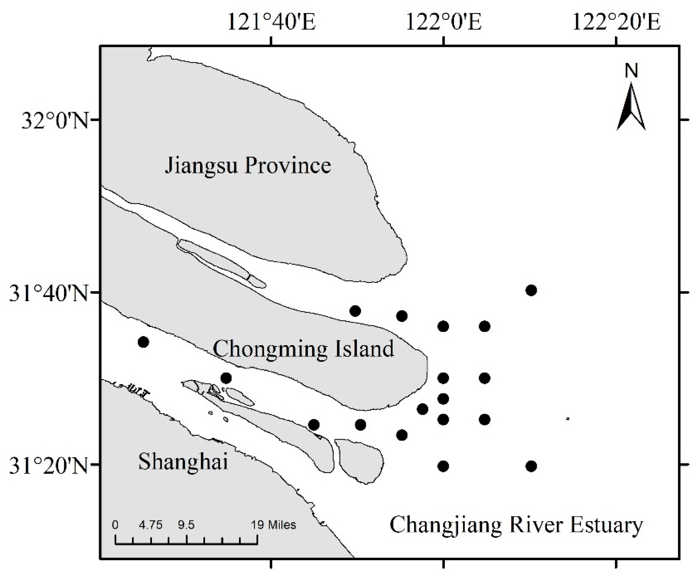
2.1. Time, Area, and Method of Investigation

Between 2009 and 2018, four surveys were conducted each year in spring (May), summer (August), autumn (November), and winter (February), for a total of 40 research surveys. The data used in this study were obtained from 18 stations in the Changjiang estuary (Figure 1). The bottom trawl used for sampling had a net width of 6 m, cod-end mesh size of 2 cm, and height of 2 m. One tow was performed at each station, at a speed of 2 nm/h for 15 min. All the catch was taken back to the laboratory for identification of the species therein and to determine the quantity of the catch. Environmental variables such as water depth (depth, m), bottom water temperature (Temp, °C), bottom salinity (salinity, mg/L), pH, and dissolved oxygen (DO, mg/L) were measured using a multi-parameter water quality meter (WTW-3430). The water samples were taken back to the laboratory to determine chlorophyll a (Chl-a, μg/L) and chemical oxygen demand (COD, mg/L). Among them, the surveys from 2010–2011 and August 2015–2016 were not selected because of a lack of environmental data; the number of sites, and data from different years of the study are shown in

Table 1. Number of sites and data volume in different years during the study.

Year	2009	2012	2013	2014	2016	2017	2018	Total
Total number of sites surveyed throughout the year	52	52	52	52	52	52	52	364
Number of sites used	52	39	46	51	5	23	36	252

.

2.2. Variables Selection

The predictive variables measured in this study were divided into spatiotemporal and environmental factors. The spatiotemporal factors including season, longitude, and latitude, and the environmental factors included depth, temperature, salinity, DO, pH, Chl-a, and COD. As there could be multicollinearity between these variables, they needed to be screened first. Correlation analysis and variance inflation factors (VIFs) were used to test the multicollinearity of variables before spatial interpolation [19,20], the environmental variables with VIF > 3 in the model were removed [21,22], and the remaining variables were used to build the model.

2.3. Model Development

In this study, a two-stage generalized additive model (GAM) was adopted to establish the relationship between various environmental variables and resource abundance of C. nasus. This model can reduce the impact of zero values [23], its predictive variables are smoothed independently, and the degree of response change is calculated in an additive way, so that the linear and nonlinear relationships between the variables can be demonstrated well [24]. The model is divided into two stages: the first stage of the GAM model estimated that the presence probability of C. nasus was a binomial error distribution, and the second stage of the GAM model used a Gaussian error distribution function to estimate the log transformation abundance of the species [25]. In this study, the number of C. nasus caught per hour in the survey was used to represent abundance, and the data were log-transformed to conform to the model assumption of normal distribution [26]. The two-stage GAM model formula is as follows:

GAM1:

logit(p) = Year + Month + s(Lon) + s(Lat) + s(Temp) + s(Depth) +
s(pH) + s(Sal) + s(Chla) + s(DO) + s(COD) + ε

(1)

GAM2:

ln(d) = Year + Month + s(Lon) + s(Lat) + s(Temp) + s(Depth) +
s(pH) + s(Sal) + s(Chla) + s(DO) + s(COD) + ε

(2)

where p is the presence probability of C. nasus, d is the abundance of C. nasus (unit: N/h), s is the spline smoothing function, Lon is the longitude of the survey site, Lat is the latitude of the survey site, Temp is water temperature, Depth is water depth (m), Sal is salinity (mg/L), Chla is chlorophyll a (mg/L), DO is dissolved oxygen (mg/L), COD is chemical oxygen demand (mg/L), and ε is the random error term. Based on the value of the smallest corrected Akaike information criterion (AIC), the variables were selected via a backward stepwise regression method [27]. The smaller the AIC, the better the fitting ability of the model [28].

Finally, combining the results of the two-stage GAM, the following formula was used to estimate the total log-abundance of C. nasus (D):

ln(D) = pln(d)

(3)

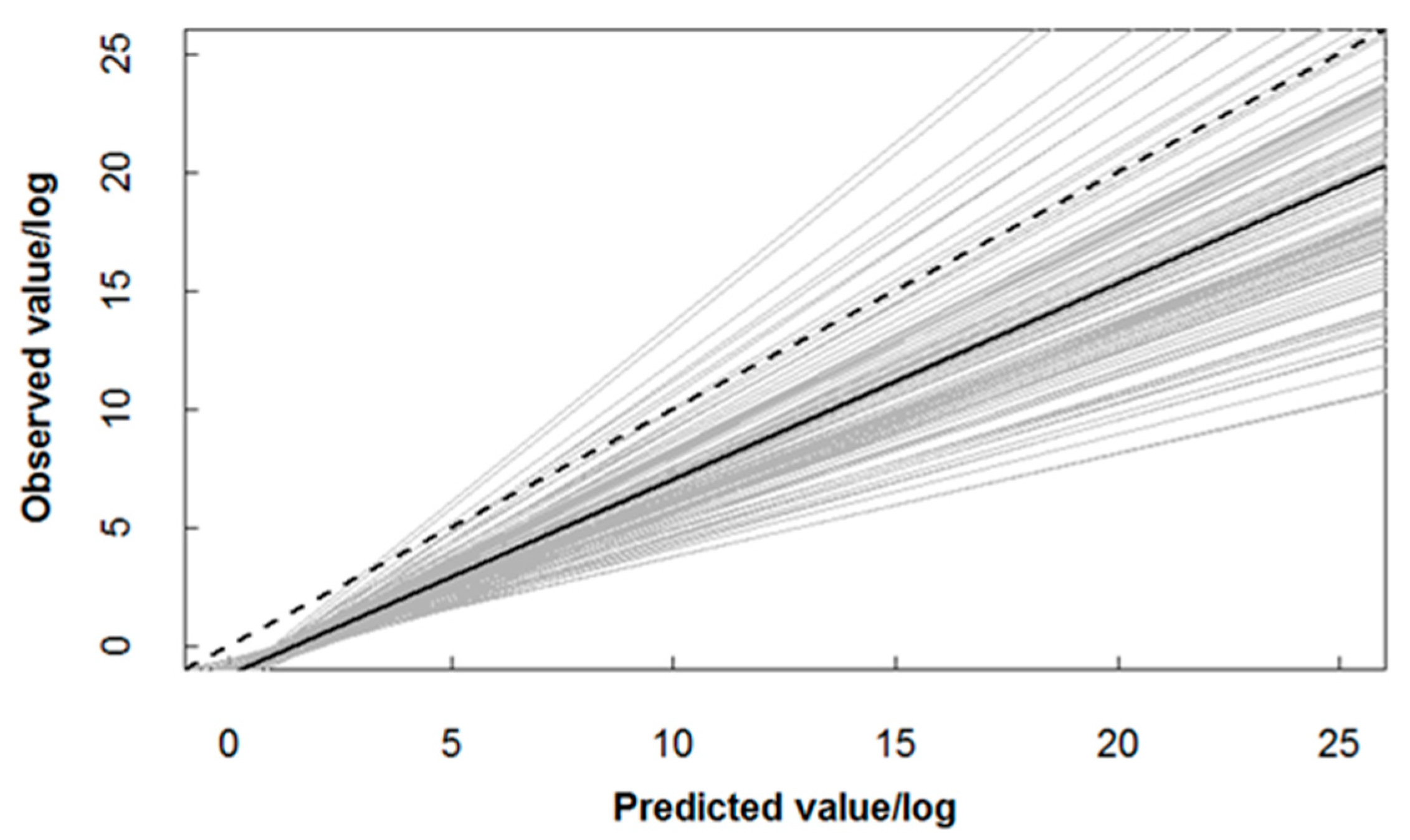
2.4. Model Validation

Cross-validation was used to verify the prediction effect of the model [29]. Several cross-validation methods are available to evaluate the model performance. In this study, k-fold cross-validation (K = 5) was used, and the number of repeats was 100 [30]. The specific steps are as follows. The data set was randomly divided into five subsets, one test set was retained, and the model was trained on all other training sets (i.e., 80% of the data were randomly selected for modeling each time, and 20% of the data were cross-verified). Then, the test set was used to verify the prediction results of the model, and the prediction errors were recorded. This process was repeated until each of the five subsets was used as a test set, and the prediction errors for the five records were averaged. Then, the above process was repeated 100 times, and the final model error was the average error of the 100 repetitions. The linear relationship of the predicted C. nasus abundance (Y) based on the model developed using training data and the observed C. nasus abundance (y) of the testing data was established using the regression model as follows:

ln(Y) = a + b × ln(y)

(4)

where the averaged a and b values indicate the bias of the model prediction. When a = 0 and b = 1, the model exhibits the best predictive performance [21,22].

2.5. Model Prediction and Mapping

As the environmental data that we used are point data from the ship survey, they needed to be converted into plane data applicable to the entire study area through a spatial interpolation method. This method can estimate the value of unknown points based on the environmental factors of sampling points [31], and change the resolution of the data [10]. Therefore, it is an effective method for obtaining the continuous distribution of environmental factors.

A study by Pan et al. (2021) compared the differences in various environmental elements obtained by different interpolation methods in the Changjiang River estuary, and recommended specific interpolation methods suitable for different environmental factors [18]. The inverse distance weighting interpolation (IDW) was adopted for the concentration of Chla, and the regularized spline function (RS) in the radial basis function (RBF) were used for the spatial interpolation of Temp and Sal. For pH, the Gaussian model (OKG) in the ordinary kriging (OK) method was used. Since COD data were not used in the study by Pan et al., OKG was used for the spatial interpolation of COD in our study.

Cross-validation was used to compare the effectiveness of interpolation. In the process of cross-validation, one of the known points is removed from the dataset, and then the value of the removed points is estimated by the other points [32]. After completing the above steps for each point, the arithmetic mean error (ME) of the prediction error is calculated as an index to evaluate the accuracy of the interpolation method. Standard deviation (SD) and coefficient of variability (CV) were used to measure the degree of variation in the data distribution after interpolation. ME reflects the overall estimation bias of the interpolation [33]. If ME is closer to zero, the predicted value is more unbiased. SD is the best indicator for measuring the degree of variation. The smaller the SD, the lower the degree of dispersion. CV is a supplementary indicator for SD and is used to compare the relative degrees of variation of different samples [34]. The calculation formulas for ME, SD, and CV are as follows:

$$\mathrm{ME}=\frac{1}{\mathrm{N}}{{\displaystyle \sum }}_{\mathrm{i}=1}^{\mathrm{n}}[\mathrm{z}({\mathrm{x}}_{\mathrm{i}})]$$

(5)

$$\mathrm{SD}=\sqrt{\frac{{{\displaystyle \sum }}_{\mathrm{i}=1}^{\mathrm{n}}{\left({\mathrm{x}}_{\mathrm{i}}-\overline{\mathrm{x}}\right)}^2}{\mathrm{n}-1}}$$

(6)

$$\mathrm{CV}=\frac{\mathrm{SD}}{\mathrm{ME}}\times 100\%$$

(7)

where z(x_i) is the predicted value of point x_i, n is the number of samples, and $\overline{\mathrm{x}}$ is the average.

After interpolation of various environmental data at different spatial resolutions (1′ × 1′, 2′ × 2′, 3′ × 3′, 4′ × 4′, 5′ × 5′; in units of minutes, 1 min = 1/60 degrees), they were input into the established two-stage GAM model to predict the spatial distribution of C. nasus in the study area, and the Arcmap 10.2 software was used for all plots (Environmental Systems Research Institute, RedLands, CA, USA).

3. Results

3.1. Model Results

Based on the VIF analysis, the VIF values of all explanatory variables were less than three, and no environmental factors needed to be deleted before the backward stepwise regression.

As shown in

Table 2. Summary of variables and model performances of the generalized additive models (GAMs).

	Predictive Variables	p Value	AIC	AUC	Deviance Explained	R2
GAM1	Month	0.016329	207.84	0.83	25.5%	0.257
	COD	0.030504
	Temp	0.054044
	Sal	0.000681
	Year	0.002734
	Lat	0.004118
GAM2	Year	0.005802	151.76		22.5%	0.172
	Lat	0.070189
	pH	0.066935
	Chla	0.000818

, after variable screening based on AIC, the optimal model of GAM1 contains six variables, and the optimal model of GAM2 contains four variables. Among them, two variables, Year and Lat, were retained, indicating that these two spatiotemporal factors would affect the existence and abundance of C. nasus. The deviance explained by GAM1 was 25.5%, AUC was 0.83, and the R² was 0.257. The deviance explained by GAM2 was 22.5%, and the R² was 0.172.

The cross-validation results showed that the intercept range of 100 cycles was −1.63 to −0.62, with an average of −1.14. The slope ranged from 0.52 to 1.46 with an average of 0.82, and the R² ranged from 0.67 to 0.89, with an average of 0.80. The linear regression between the observed and fitted values of the 100 cross-validations is shown in Figure 2.

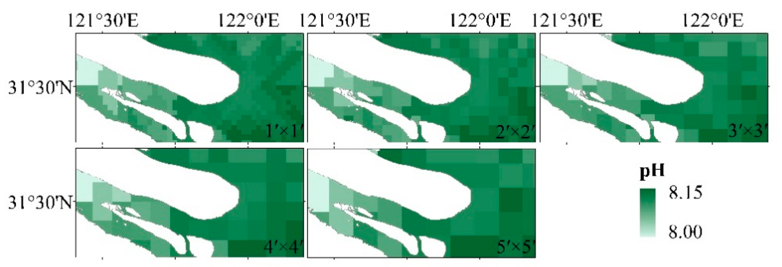
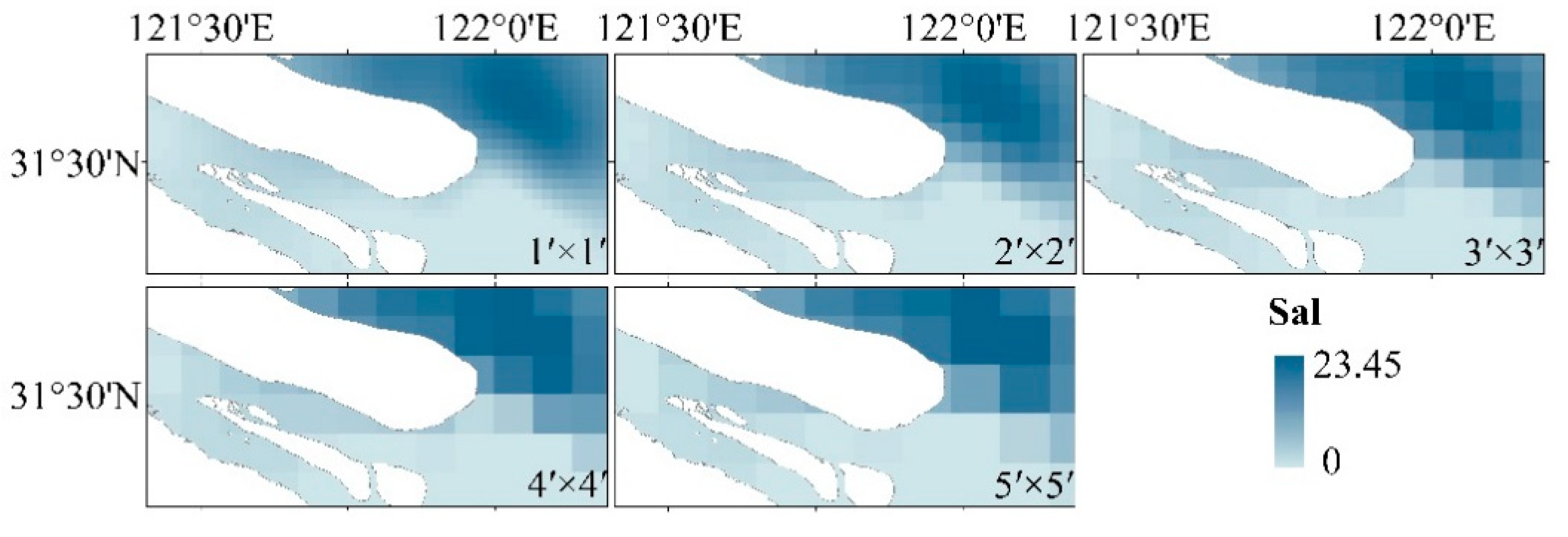
3.2. Interpolation Analysis of Environmental Factors

The mean value (ME), standard deviation (SD), and CV of environmental factors changed after interpolation (see

Table 3. Descriptive analysis of environment variables in different spatial interpolation methods.

Spatial Scale	Chlorophyll a/μg·L−1		CV	pH		CV
	Mean (Range)	SD		Mean (Range)	SD
True	1.781 (0.086–11.250)	1.975	1.109	8.013 (6.620–9.032)	0.368	0.0459
1′ × 1′	1.920 (0.104–11.250)	2.040	1.063	8.018 (7.142–8.596)	0.263	0.0328
2′ × 2′	1.922 (0.104–11.250)	2.041	1.062	8.017 (7.153–8.555)	0.264	0.0329
3′ × 3′	1.872 (0.105–11.250)	2.072	1.107	8.001 (7.137–8.549)	0.264	0.0330
4′ × 4′	1.919 (0.111–11.250)	2.045	1.066	8.018 (7.213–8.549)	0.261	0.0326
5′ × 5′	1.925 (0.112–11.250)	2.071	1.076	8.017 (7.203–8.549)	0.264	0.0329
Spatial Scale	COD/mg·L−1		CV	Salinity/mg·L−1		CV
	Mean (Range)	SD		Mean (Range)	SD
True	1.034 (0.400–1.600)	0.470	0.455	9.112 (0.000–29.800)	10.077	1.106
1′ × 1′	0.962 (0.410–1.618)	0.281	0.292	7.754 (0.000–34.687)	7.700	0.993
2′ × 2′	0.963 (0.430–1.614)	0.281	0.292	7.771 (0.000–34.777)	7.703	0.991
3′ × 3′	0.964 (0.464–1.608)	0.284	0.294	7.853 (0.000–34.272)	7.719	0.983
4′ × 4′	0.963 (0.479–1.603)	0.290	0.301	7.893 (0.000–34.314)	7.748	0.982
5′ × 5′	0.948 (0.485–1.616)	0.285	0.301	8.135 (0.000–32.396)	7.790	0.958
Spatial Scale	Water Temperature/°C				CV
	Mean (Range)			SD
True	18.168 (5.600–30.100)			8.002	0.4404
1′ × 1′	18.098 (5.442–30.528)			7.892	0.4361
2′ × 2′	18.098 (5.446–30.526)			7.894	0.4362
3′ × 3′	18.015 (5.468–30.157)			7.819	0.4340
4′ × 4′	18.103 (5.475–30.512)			7.895	0.4361
5′ × 5′	18.118 (5.448–30.525)			7.893	0.4356

Note: SD—standard deviation. CV—the coefficient of variation. True—measured values.

). For certain variables, the ME and SD of Chla became larger after interpolation, and CV became smaller, indicating that the degree of dispersion increased after interpolation. After the interpolation, the ME of pH became larger when divided by 3′ × 3′, the SD decreases, and the CV decreases, indicating that the degree of dispersion decreases after the interpolation. The ME, SD, and CV of COD decreased after interpolation, indicating that the degree of dispersion decreased after interpolation. The results of the Sal and Temp interpolations were similar to those of COD.

The values of the environmental factors obtained by interpolation at different spatial resolutions also differed (see Table 3). The ME of Chl-a at 3′ × 3′ was significantly lower than that at other spatial scales, but it was closer to the true value, and the values of SD and CV were higher than those at other scales, indicating that the degree of dispersion of Chla was higher than that at other scales. The ME of the predicted pH at 3′ × 3′ was significantly lower than that at other spatial scales, and the difference from the true value was larger. The mean value of COD predicted at 5′ × 5′ was lower than that at other scales. The ME of the predicted value of Sal under 5′ × 5′ was higher than that of other spatial scales, and was closer to the true value. The ME of the predicted value of Temp at 3′ × 3′ was significantly lower than that at other spatial scales and had a large gap with the true value. The SD and CV were smaller than those at other scales, indicating that the degree of dispersion was lower than that at other scales.

The environmental factors differed with the spatial resolution, but the overall distribution trend of the environmental factors did not vary. For example, Chl-a and pH were higher outside the Changjiang River estuary. The Temp and COD of the southern branch of the estuary were higher, whereas the northern branch of the estuary had higher Sal. For environmental factors such as pH, which vary little in the estuary and have marginal difference between the highest and the lowest values, small changes can be observed in the interpolation results at a small scale. The interpolation results under 1′ × 1′ were similar to those under 2′ × 2′, and the interpolation results under 3′ × 3′ were similar to those under 4′ × 4′. The interpolation results at 5′ × 5′ were different from the distribution details at a small scale (Figure 3). However, for environmental factors such as Sal, which vary dramatically in the estuary and differ greatly from the highest to the lowest value, the distribution characteristics were similar at all scales (Figure 4).

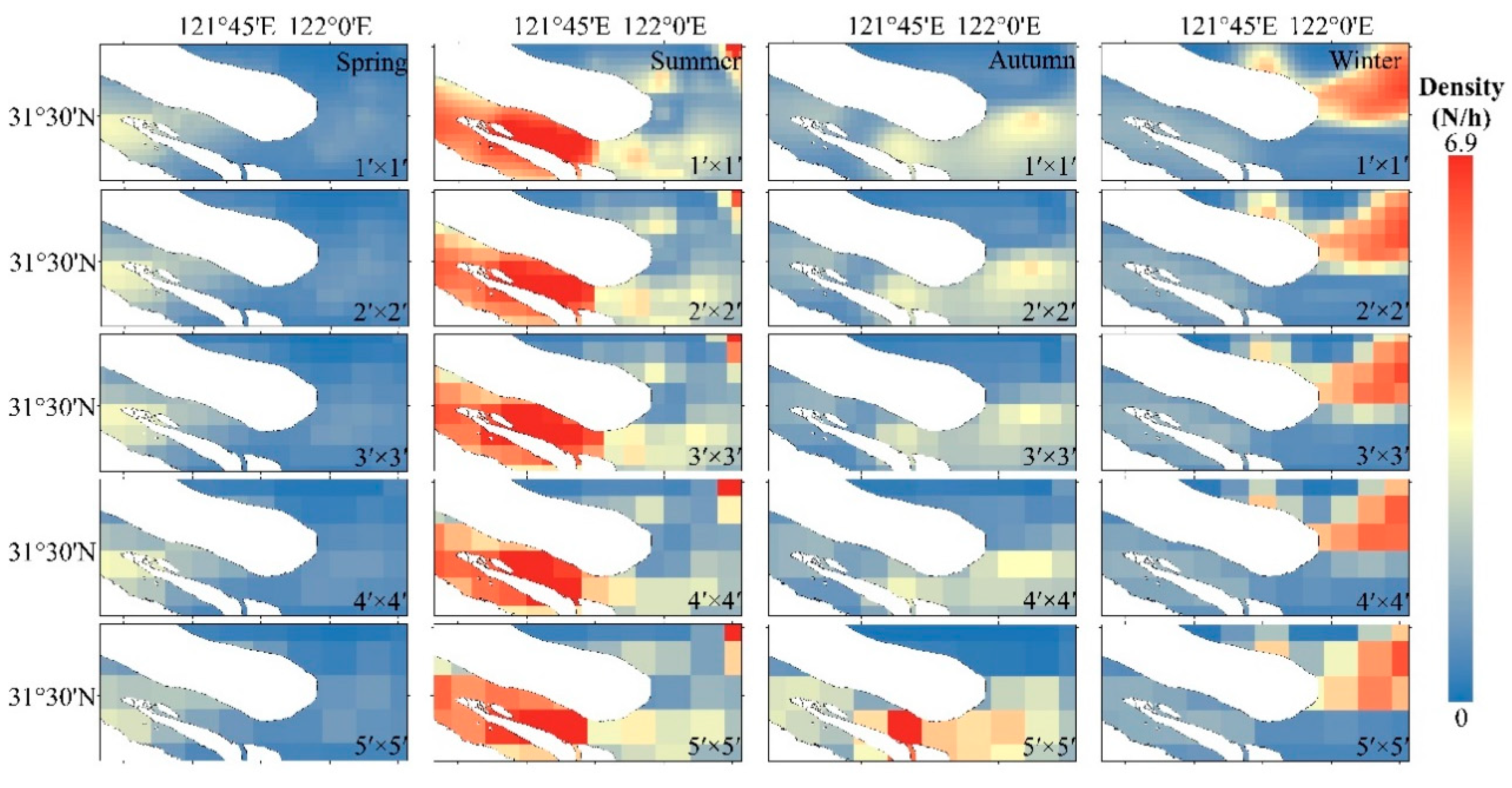
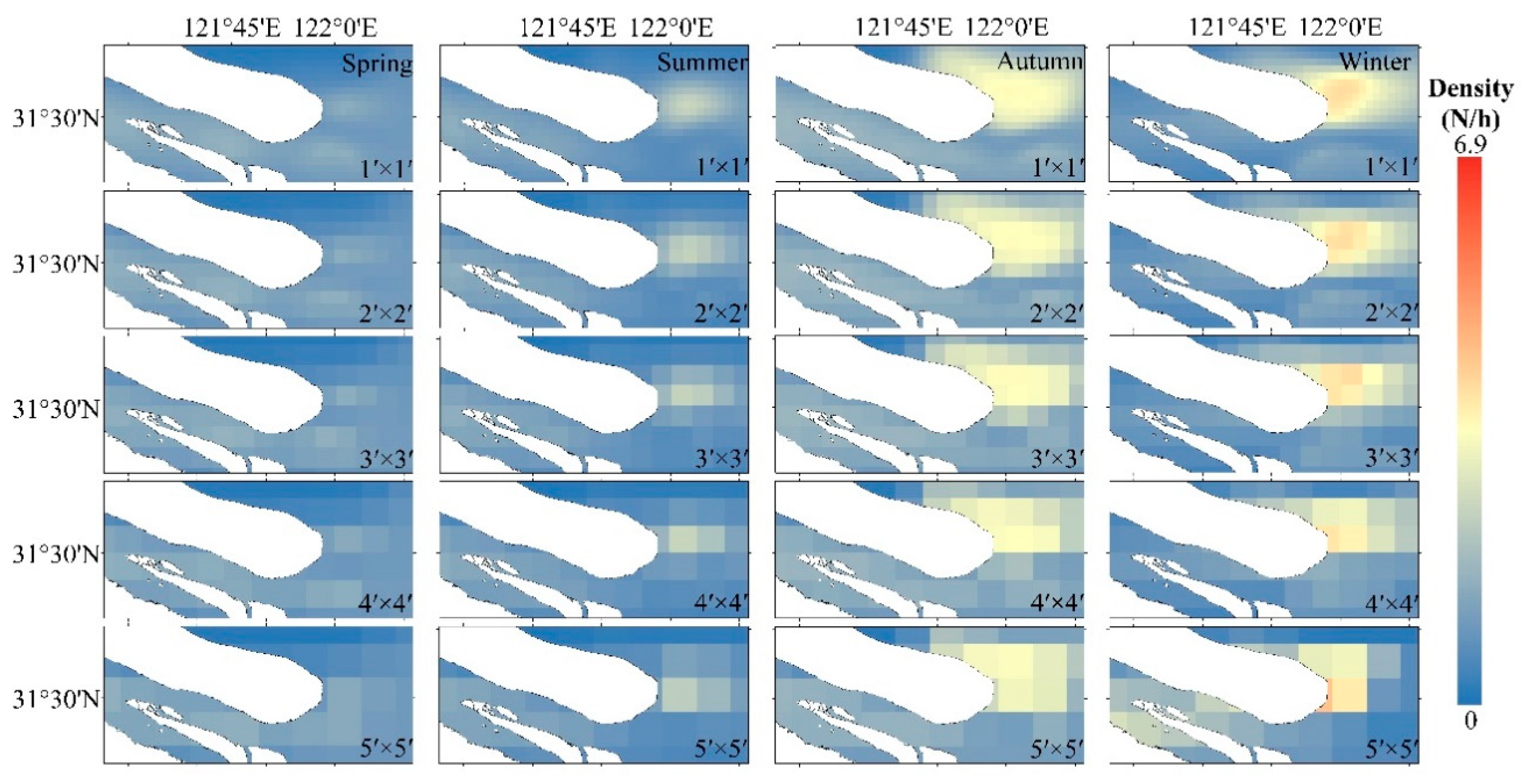
3.3. Prediction of Spatial and Temporal Distribution of C. nasus

By comparing the spatial distribution characteristics of C. nasus at different scales, it was observed that, in most cases, the prediction results of various spatial scales at the same period were similar (Figure 5, Figure 6 and Figure 7). Taking each season from 2012 to 2014 as an example, the prediction results for all scales in 2013 and 2014 were very similar, and changes in spatial scale had marginal impact on the final prediction results (Figure 6 and Figure 7). In 2012, except for the forecast of 5′ × 5′ in autumn, the distribution pattern of C. nasus in the same season was roughly similar. In autumn and winter, the species was mainly distributed in the outer waters near the sea of Chongming Island, and its distribution expanded to the adjacent river areas. In spring and summer, it was mainly distributed in the freshwaters inside the estuary, and the annual peak occurred in summer (Figure 5). However, in the autumn of 2012, the distribution center of C. nasus showed a trend of gradually moving southward, from the small to large scale and reached the extreme at the 5′ × 5′ scale. The high-abundance area not only moved southward, but also showed a clear expansion. The highest abundance area was transferred to the river in the southern branch of the Changjiang River. This is significantly different from the spatial characteristics of the highest abundance at the other scales (Figure 5).

4. Discussion

4.1. Predictive Performance of the Two-Stage GAM Model for C. nasus Distribution

The two-stage GAM model is a statistical model that is often used to establish the relationship between environmental factors and species distribution. This is applicable to situations with many zero values. For example, Jensen et al. (2005) used this method to study the distribution pattern of blue crab (Callinectes sapidus) in Chesapeake Bay, USA, in winter, and used regression to verify the advantages and disadvantages of the model, and found unique habitat relationships in certain years [35]. Lubnah et al. (2008) used this method to analyze the distribution and abundance of emperor fish (Lethrinus spp.) in the Arabian Sea to confirm the robustness of the original data [36]. Chang et al. (2010) used this approach to quantify spatial distributions of lobsters, according to the season, size, and sex, in the Gulf of Maine based on environmental and spatial variables. They provided an excellent tool for assessing changes in spatial distributions of lobsters relative to primary habitats and other environmental variables [25].

According to the cross-validation results of this study, the prediction performance of this model was good, but the prediction performance for low abundance was better than that for high abundance (Figure 2). A possible reason is that the abundance of C. nasus, at most sampling sites in the study area, was very low, and the data with high abundance accounted for a small proportion of the original data used for modeling, which led to a better prediction performance of the model for low abundance. In addition, Ciannelli et al. (2007) reported the possibility that, in the process of fish aggregation, there were some non-linear and non-additive processes affecting fish aggregation, which could not be fully explained by the GAM model [37]. However, in general, the prediction results of the two-stage GAM model established in this study can be used to compare the distribution characteristics of C. nasus in the Changjiang River Estuary at different spatial scales.

4.2. The Relationship between the Interpolation Results between Environmental Factors and Spatial Scale

Spatial interpolation is a common method for obtaining the distribution of marine environmental elements in estuarine and coastal waters, and the related process and details of spatial interpolation determine the interpolation results [18]. Pan et al. (2021) compared the differences caused by the selection of IDW, RS, OK and other interpolation methods on the prediction results of spatial distribution of resources in the Changjiang River estuary [18]. However, the potential impact of scale selection on environmental factors has not been analyzed. Our results suggest that in the Changjiang River estuary region, for environmental factors that little in the estuary region, and with marginal difference between the highest and lowest values (such as pH), the interpolation results on a small scale can well reflect the variation details of their spatial characteristics (Figure 3). This may be related to the adsorption of phosphates by sediments in the Changjiang River estuary [38]. Due to the complex sediment exchange between the Changjiang River estuary and the nearby coast, pH changes occur at a micro scale [39]. However, for environmental factors such as salinity, which vary dramatically in the estuarine region and have a relatively large difference between the highest and lowest values, the interpolation results, at small scales, were not significantly different from those at other scales (Figure 4). These findings suggest that the sensitivity of environmental factors depends on the spatial scale, and that the spatial scale selection of the more sensitive environmental factors may further play a role in certain processes involved in prediction of species distribution.

4.3. The Relationship between Fish Resource Forecasts and Spatial Scale

The selection of the optimal spatial scale is often evaluated using a multi-scale approach, which has the advantage of ensuring that the distribution of organisms is understood at an appropriate scale [40]. For example, Maravelias et al. (2001) used the GAM model to consider the habitat associations of Atlantic herring (Clupea harengus) with a range of biological and abiotic factors at three different spatial scales [41]. They reported that a basic sampling distance of 2.5 nautical miles (ESDU) is a reasonable sampling scheme. It reduces the need for a high volume of data while maintaining a spatial resolution large enough to distinguish species in relation to their environment. Song et al. (2012) used the MaxEnt model to assess the sensitivity of species distribution modeling to different spatial scales ranging from 30 m to 4950 m [42]. The results of this study indicate that the maximum spatial scale should be approximately 1.5 km, and that the prediction accuracy decreases if the sampling scale is greater than 1.5 km.

Coilia nasus in the Changjiang River is a typical migratory fish. Every spring, mature individuals of C. nasus enter the river in groups from the sea and migrate up the river for reproduction. The hatchlings of the species float downstream and live in the brackish water in the estuary in the first year, and mature and reside in the sea in the second year [43]. Therefore, occurrence over time of C. nasus in the estuary showed significant seasonal and interannual variations. From previous studies, water temperature has always been an important environmental factor affecting the distribution of fish in estuaries [44]. Temperature may be triggering pre-spawning migration behavior in C. nasus [45]. Our results also showed that the C. nasus had a tendency of spreading from offshore to inland in spring when the temperature rose, indicating that the C. nasus had entered the process of reproductive migration. Previous studies on C. nasus found that pH also affected its distribution, and weakly alkaline water (8.5–9.5) was more suitable for the survival of C. nasus [46]. At the same time, the increase of chlorophyll in a certain range (5–15 μg·L⁻¹) also increased the abundance of C. nasus [47]. Moreover, estuaries are heterogeneous environments, which consist of many distinctive habitat types, and fish species may actively select the most appropriate one for spawning [48]. The comparative results of multi-scale spatial distribution prediction of C. nasus in the Changjiang River estuary in this study show that, except for individual spatial scales in certain years, the spatial distribution patterns of C. nasus predicted, simultaneously at different scales, are very similar. Further, the spatial distribution at different scales can reflect the quarterly and inter-annual variation trends of spatial characteristics (Figure 5, Figure 6 and Figure 7). The conditions in which a prediction occurs at one scale are occasionally different from those at other scales. For example, in autumn 2012, the maximum abundance of C. nasus at the scale of 5′ × 5′ occurred in the waters of the southern branch of the estuary and expanded significantly (Figure 5). Hastie et al. (1990) suggested that this is possibly due to the fact that, although the differences of environmental factors interpolated at different spatial scales were small, these differences were amplified during the process of integration of various factors for the iterative prediction of the GAM model [49]. Therefore, the selection of a spatial scale may influence the prediction of species distribution in some cases.

5. Outlook

The studies on spatial scales of biological reactions are still in their infancy [50]. In our study, it is difficult to explain the specific causes of pH changes, and it is suggested to conduct more detailed research thereupon in the future. In our study, because the prediction at a small scale can more intuitively reflect the specific details of fish distribution in a relatively small area and provide more information for the delineation of protection space in estuarine areas, we suggest that smaller scales should be chosen whenever possible, considering the calculation difficulty thereof. Currently, there are few studies on the selection of optimal spatial scales for different fish in the Changjiang River estuary region, and the subject of this study was a typical migratory fish. Therefore, we suggest that targeted studies should be carried out in the future to determine whether this conclusion is directly applicable to other fish. At the same time, attention should be paid to the selection of spatial scales in estuarine regions, particularly in sites without any existing data. It is hoped that our research can provide a basis for the studies on spatial scales of biological reactions.

References

1. Legendre, P.; Fortin, M.J. Spatial pattern and ecological analysis. Vegetatio 1989, 80, 107–138. [Google Scholar] [CrossRef]
2. Zhao, J.; Zhang, S.Y.; Wang, Z.H.; Lin, J.; Zhou, X.J. Fish community diversity distribution and its affecting factors based on GAM model. Chin. J. Ecol. 2013, 32, 3226–3235. [Google Scholar]
3. Allen, L.G.; Daniel, I.I.; Shane, M.A. Fisheries independent assessment of a returning fishery: Abundance of juvenile white seabass (Atractoscion nobilis) in the shallow nearshore waters of the Southern California Bight, 1995–2005. Fish. Res. 2007, 88, 24–32. [Google Scholar] [CrossRef]
4. Bacha, M.; Jeyid, M.A.; Vantrepotte, V.; Dessailly, D.; Amara, R. Environmental effects on the spatio-temporal patterns of abundance and distribution of Sardina pilchardus and sardinella off the Mauritanian coast (North-West Africa). Fish. Oceanogr. 2017, 26, 282–298. [Google Scholar] [CrossRef]
5. Fahrig, L. Relative Importance of Spatial and Temporal Scales in a Patchy Environment. Theor. Popul. Biol. 1992, 41, 300–314. [Google Scholar] [CrossRef]
6. Hale, R.; Colton, M.A.; Peng, P.; Swearer, S.E. Do spatial scale and life history affect fish–habitat relationships? J. Anim. Ecol. 2019, 88, 439–449. [Google Scholar] [CrossRef]
7. Basher, Z.; Bowden, D.A.; Costello, M.J. Diversity and distribution of deep-sea shrimps in the Ross Sea region of Antarctica. PLoS ONE 2014, 9, e103195. [Google Scholar] [CrossRef] [Green Version]
8. Crook, D.A.; Robertson, A.I.; King, A.J.; Humphries, P. The influence of spatial scale and habitat arrangement on diel patterns of habitat use by two lowland river fishes. Oecologia 2001, 129, 525–533. [Google Scholar] [CrossRef]
9. Petitgas, P. Allocation of survey effort between small scale and large scale and precision of fisheries survey-based abundance estimates. ICES CM 2001, 17. Available online: https://www.ices.dk/sites/pub/CM%20Doccuments/2001/P/P1701.pdf (accessed on 7 October 2021).
10. Rufino, M.M.; Bez, N.; Brind’Amour, A. Influence of data pre-processing on the behavior of spatial indicators. Ecol. Indic. 2019, 99, 108–117. [Google Scholar] [CrossRef]
11. Zhang, T.T.; Gao, Y.; Wang, S.K.; Liu, J.Y.; Zhang, T.; Song, C.; Zhao, F.; Zhuang, P. Landscape pattern of estuarine wetland and its multi-scale effects on macrobenthos diversity. Mar. Fish. 2018, 40, 679. [Google Scholar]
12. Alam, R.Q.; Benson, B.C.; Visser, J.M.; Gang, D.D. Response of estuarine phytoplankton to nutrient and spatio-temporal pattern of physico-chemical water quality parameters in Little Vermilion Bay, Louisiana. Ecol. Inform. 2016, 32, 79–90. [Google Scholar] [CrossRef]
13. Rivoirard, J.; Wieland, K. Correcting for the effect of daylight in abundance estimation of juvenile haddock (Melanogrammus aeglefinus) in the North Sea: An application of kriging with external drift. ICES J. Mar. Sci. 2001, 58, 1272–1285. [Google Scholar] [CrossRef] [Green Version]
14. Zhuang, P. Fishes of Yangtze Estuary; China Agriculture Press: Beijing, China, 2018. [Google Scholar]
15. Yuan, X.Z.; Liu, H.; Lu, J.J. The ecological and environmental characteristics and conservation of the wetlands in the Changjiang Estuary, China. Environmentalist 2002, 22, 311–318. [Google Scholar] [CrossRef]
16. Jing, Y.H. The Characteristics of Estuarine in China. Donghai Mar. Sci. 1988, 3, 5–15. [Google Scholar]
17. Dai, L.B.; Hodgdon, C.; Tian, S.Q.; Cheng, J.H.; Gao, C.X.; Han, D.Y.; Kindong, R.; Ma, Q.Y.; Wang, X.F. Comparative performance of modelling approaches for predicting fish species richness in the Yangtze River Estuary. Reg. Stud. Mar. Sci. 2020, 35, 101161. [Google Scholar] [CrossRef]
18. Pan, S.Y.; Tian, S.Q.; Wang, X.F.; Dai, L.B.; Gao, C.X.; Tong, J.F. Comparing different spatial interpolation methods to predict the distribution of fishes: A case study from Coilia nasus in the Changjiang River Estuary. Acta Oceanol. Sin. 2021, 40, 119–132. [Google Scholar] [CrossRef]
19. Liu, X.X.; Wang, J.; Zhang, Y.L.; Yu, H.; Xu, B.; Zhang, C.L.; Ren, Y.P.; Xue, Y. Comparison between two GAMs in quantifying the spatial distribution of Hexagrammos otakii in Haizhou Bay, China. Fish. Res. 2019, 218, 209–217. [Google Scholar] [CrossRef]
20. Shepard, D. A two-dimensional interpolation function for irregularly-spaced data. In Proceedings of the 1968 23rd ACM National Conference, New York, NY, USA, 27–29 August 1968; pp. 517–524. [Google Scholar]
21. Sagarese, S.R.; Frisk, M.G.; Cerrato, R.M.; Sosebee, K.A.; Musick, J.A.; Rago, P.J. Application of generalized additive models to examine ontogenetic and seasonal distributions of spiny dogfish (Squalus acanthias) in the Northeast (US) shelf large marine ecosystem. Can. J. Fish. Aquat. Sci. 2014, 71, 847–877. [Google Scholar] [CrossRef]
22. Thomson, R.E.; Emery, W.J. Data Analysis Methods in Physical Oceanography; Newnes: Oxford, UK, 2014. [Google Scholar]
23. Li, B.; Cao, J.; Chang, J.H.; Wilson, C.; Chen, Y. Evaluation of effectiveness of fixed-station sampling for monitoring American lobster settlement. N. Am. J. Fish. Manag. 2015, 35, 942–957. [Google Scholar] [CrossRef]
24. Wood, S.N.; Augustin, N.H. GAMs with integrated model selection using penalized regression splines and applications to environmental modelling. Ecol. Model. 2002, 157, 157–177. [Google Scholar] [CrossRef] [Green Version]
25. Chang, J.H.; Chen, Y.; Holland, D.; Grabowski, J. Estimating spatial distribution of American lobster Homarus americanus using habitat variables. Mar. Ecol. Prog. Ser. 2010, 420, 145–156. [Google Scholar] [CrossRef]
26. Barry, S.C.; Welsh, A.H. Generalized additive modelling and zero inflated count data. Ecol. Model. 2002, 157, 179–188. [Google Scholar] [CrossRef]
27. Strawderman, R.L. Model selection and inference: A practical information-theoretic approach. J. Am. Stat. Assoc. 2000, 95, 341. [Google Scholar] [CrossRef]
28. Planque, B.; Bellier, E.; Lazure, P. Modelling potential spawning habitat of sardine (Sardina pilchardus) and anchovy (Engraulis encrasicolus) in the Bay of Biscay. Fish. Oceanogr. 2007, 16, 16–30. [Google Scholar] [CrossRef]
29. Rodriguez, J.D.; Perez, A.; Lozano, J.A. Sensitivity analysis of k-fold cross validation in prediction error estimation. IEEE Trans. Pattern Anal. Mach. Intell. 2009, 32, 569–575. [Google Scholar] [CrossRef]
30. Kohavi, R. A study of cross-validation and bootstrap for accuracy estimation and model selection. Ijcai 1995, 14, 1137–1145. [Google Scholar]
31. Appice, A.; Malerba, D. Leveraging the power of local spatial autocorrelation in geophysical interpolative clustering. Data Min. Knowl. Disc. 2014, 28, 1266–1313. [Google Scholar] [CrossRef]
32. Mueller, T.G.; Pusuluri, N.B.; Mathias, K.K.; Cornelius, P.L.; Barnhisel, R.I.; Shearer, S.A. Map quality for ordinary kriging and inverse distance weighted interpolation. Soil Sci. Soc. Am. J. 2004, 68, 2042–2047. [Google Scholar] [CrossRef]
33. Stow, C.A.; Jolliff, J.; McGillicuddy, D.J., Jr.; Doney, S.C.; Allen, J.I.; Frtendrichs, M.A.M.; Rose, K.A.; Wallhead, P. Skill assessment for coupled biological/physical models of marine systems. J. Marine Syst. 2009, 76, 4–15. [Google Scholar] [CrossRef] [Green Version]
34. Ott, R.L.; Longnecker, M.T. An Introduction to Statistical Methods and Data Analysis; Cengage Learning: Boston, MA, USA, 2015. [Google Scholar]
35. Jensen, O.P.; Seppelt, R.; Miller, T.J.; Bauer, L.J. Winter distribution of blue crab Callinectes sapidus in Chesapeake Bay: Application and cross-validation of a two-stage generalized additive model. Mar. Ecol. Prog. Ser. 2005, 299, 239–255. [Google Scholar] [CrossRef] [Green Version]
36. Al-Kharusi, L.H. Predicting the distribution and abundance of emperor fishes (Lethrinus spp.) in the Arabian Sea using two-stage generalized additive models and a geographic information system. J. Agr. Mar. Sci. 2008, 13, 7–22. [Google Scholar] [CrossRef] [Green Version]
37. Ciannelli, L.; Fauchald, P.; Chan, K.S.; Agostini, V.N.; Dingsør, G.E. Spatial fisheries ecology: Recent progress and future prospects. J. Mar. Syst. 2008, 71, 223–236. [Google Scholar] [CrossRef]
38. Bostrom, B. Relations between chemistry, microbial biomass and activity in sediments of a polluted vs. a nonpolluted eutrophic lake. Verh. Int. Ver. Limnol. 1988, 23, 451–459. [Google Scholar] [CrossRef]
39. Andersen, J.M. Nitrogen and phosphorus budgets and the role of sediments in six shallow Danish lakes. Arch. Hyd. 1974, 74, 527–550. [Google Scholar]
40. Jackson, H.B.; Fahrig, L. What size is a biologically relevant landscape? Landsc. Ecol. 2012, 27, 929–941. [Google Scholar] [CrossRef]
41. Maravelias, C.D. Habitat associations of Atlantic herring in the Shetland area: Influence of spatial scale and geographic segmentation. Fish. Oceanogr. 2001, 10, 259–267. [Google Scholar] [CrossRef]
42. Song, W.; Kim, E.; Lee, D.; Lee, M.; Jeon, S. The sensitivity of species distribution modeling to scale differences. Ecol. Model. 2013, 248, 113–118. [Google Scholar] [CrossRef]
43. Huang, R.S. Biological characteristics, resource status and protection countermeasures of Coilia nasus. Res. Fish. 2005, 25, 33–37. [Google Scholar]
44. Guo, H.Y.; Zhang, X.G.; Tang, W.Q.; Li, H.H.; Shen, L.H.; Zhou, T.S.; Liu, D. Temporal variations of Coilia nasus catches at jingjiang section of the Yangtze river in fishing season in relation to environmental factors. Res. Environ. Yangtze Basin 2016, 25, 1850–1859. [Google Scholar]
45. Yuan, C.M. Spawn migration of Coilia nasus. B Biol. 1978, 12, 1–3. [Google Scholar]
46. Ma, J.; Li, B.; Zhao, J.; Wang, X.F.; Hodgdon, C.T.; Tian, S.Q. Environmental influences on the spatio-temporal distribution of Coilia nasus in the Yangtze River estuary. J. Appl. Ichthyol. 2020, 36, 315–325. [Google Scholar] [CrossRef]
47. Wu, J.H.; Dai, L.B.; Dai, X.J.; Tian, S.Q.; Liu, J.; Chen, J.H.; Wang, X.F.; Wang, J.Q. Comparison of generalized additive model and boosted regression tree in predicting fish community diversity in the Yangtze River Estuary, China. J. Appl. Ecol. 2019, 30, 644–652. [Google Scholar]
48. Inui, R.; Onikura, N.; Kawagishi, M.; Makatani, M.; Oikawa, S. Selection of spawning habitat by several gobiid fishes in the subtidal zone of a small temperate estuary. Fish. Sci. 2010, 76, 83–91. [Google Scholar] [CrossRef]
49. Hastie, T.; Tibshirani, R. Generalized Additive Models; Chapman and Hall: New York, NY, USA, 1990. [Google Scholar]
50. Miguet, P.; Jackson, H.B.; Jackson, N.D.; Martin, A.E.M.; Fahrig, L. What determines the spatial extent of landscape effects on species? Landsc. Ecol. 2016, 31, 1177–1194. [Google Scholar] [CrossRef]
Figure 1. Spatial distribution of survey stations in the Changjiang River Estuary (Black dots represent the survey sites).
Fishes 06 00048 g001
Figure 2. Linear regression lines for the models from averaging 100 runs of cross-validations (the light gray solid lines are 100 linear regression lines, the black solid line is the mean of cross-validation results, and the black dashed line is the 1:1 line).
Fishes 06 00048 g002
Figure 3. Spatial distribution of the pH at different spatial resolutions in the autumn of 2014 in the Changjiang River estuary.
Fishes 06 00048 g003
Figure 4. Spatial distribution of the salinity with different spatial resolutions in the autumn of 2014 of the Changjiang River estuary.
Fishes 06 00048 g004
Figure 5. Spatial distribution of Coilia nasus predicted using interpolated environmental variables from different spatial resolutions in 2012 in the Changjiang River estuary.
Fishes 06 00048 g005
Figure 6. Spatial distribution of Coilia nasus predicted using interpolated environmental variables from different spatial resolutions in 2013 in the Changjiang River estuary.
Fishes 06 00048 g006
Figure 7. Spatial distribution of Coilia nasus predicted using interpolated environmental variables from different spatial resolutions in 2014 in the Changjiang River estuary.
Fishes 06 00048 g007