
Spatial and Temporal Variability of Parasite Communities: Implications for Fish Stock Identification


1
Programa de Doctorado en Ciencias Aplicadas, Mención Sistemas Marinos Costeros, Universidad de Antofagasta, Antofagasta 1270300, Chile
2
Escuela Nacional de Estudios Superiores Unidad Mérida (ENES-Mérida), Universidad Nacional Autónoma de México, Kilómetro 4.5 Carretera Mérida-Tétiz, Municipio de Ucú, Yucatán 97357, Mexico
3
Instituto Ciencias Naturales Alexander von Humboldt, Universidad de Antofagasta, Antofagasta 1270300, Chile
4
Millennium Institute of Oceanography (IMO), Universidad de Concepción, Concepción 4030000, Chile
*
Author to whom correspondence should be addressed.
Fishes 2021, 6(4), 71; https://0-doi-org.brum.beds.ac.uk/10.3390/fishes6040071
Submission received: 20 October 2021
/
Revised: 23 November 2021
/
Accepted: 29 November 2021
/
Published: 3 December 2021
(This article belongs to the Section Fishery Economics, Policy, and Management)
Abstract
:The spatial and temporal variability of parasite communities have received little attention when used as biological tags for identifying fish stocks. This study evaluated the potential spatial and temporal variability of the parasite communities affecting three marine fish species collected between 1993 and 2017. To avoid the potential effect of host age in parasite communities, individuals of similar ages were selected: 1123 Engraulis ringens (12–24 months old), 1904 Trachurus murphyi (24–36 months old), and 630 Merluccius gayi (36–48 months old). Most taxa show differences in the prevalence at the spatial and temporal scales, but the prevalence of some larval endoparasites remains constant at the temporal scale. At the spatial scale, an analysis of similarity (ANOSIM) showed differences in the parasite communities of three species; a canonical analysis of principal coordinates (CAP) showed low values of correct allocations (CA; ≈50%) and values of allocation due to chance (AdC) were lower than the CA. At the temporal scale, an ANOSIM showed differences between the three species. A CAP showed low values of CA (≈50–60%) and the AdC was always lower than CA. Samples at the spatial scale were well allocated to their localities or nearby localities, suggesting a spatial stability. Samples from different years were not well discriminated, suggesting temporal variability. Therefore, in studies regarding parasites as a tool for stock identification, temporal variability must be taken into account.

1. Introduction
Fishery management units are spatially defined by geographic or fishing grounds, but conventional stock assessment models assume that a fishery resource is a single, homogeneous population [1] with similar population parameters such as growth rate, recruitment, maturity and mortality; in addition, young fish in a group are produced by previous generations of the same group [2]. However, when evidence supports differences in population parameters in different areas (stocks), those must be assessed and subsequently managed as independent units [3]. Consequently, a requisite for the evaluation and posterior management of fish stocks is the correct identification [2]. The complexities of marine ecosystems present many challenges for defining population structures; hence, a variety of tools have been developed for stock identification, including: physical and electronic tags; morphometric and meristic variation; morphology and/or the chemical composition of otoliths; genetic molecular analysis; and parasite burdens [1].
Parasites have been successfully used in stock identification [4]. Nevertheless, since the pioneering studies [5,6] to the present [7,8,9], the criteria for using parasites as biological tags (BT) for stock identification have changed and evolved [10,11]. The features that parasites must present to be considered BTs, the procedures and methods for their application and their advantages and limitations have received much attention, including as the subject of many reviews [10,12,13]. Nevertheless, despite the potential spatial and temporal variability in parasite fauna being a key issue in fish stock identification, such variability has received much less attention [14,15,16].
The importance of spatial variability is clear. Spatial variability in the composition and abundance of parasite assemblages makes the use of parasites as BTs for fish stock identification possible [15,16,17]. If the loads and species of the parasites of two groups of fish are similar, then they are likely to have had a common history; if their loads are significantly different from another group, then the groups are likely to have had a different life history [18]. However, variability in parasite fauna does not necessarily mean that fish with different parasite loads belong to different stocks [19]. To assess the variability in a community, the magnitude of the study area must be considered [20].
In stock identification using parasites as BTs, caution must be taken when analyzing localities that are 100 km or less apart [21]. That is, to capture local variability, samples in locations separated by less than 100 km should be studied. Temporal variability must also be taken into account to consider a parasite as a good BT—levels of infection should remain relatively constant from year to year [12]. However, differences in infection levels within the same population may be greater over time than the differences between populations [22]. It has been suggested that before making large-scale spatial comparisons, it is necessary to have estimates of small-scale spatial variation [23]. Therefore, to reliably infer a fish stock’s structure based on parasitological data, an adequate replication of sampling at various spatial and temporal scales is needed [24]. Comparative studies over long periods require a high degree of temporal repeatability in the composition and structure of parasite communities [15,25]. Likewise, parasite communities vary through the ontogeny of their hosts, as communities in older hosts are more predictable, and ontogenetic variations should also be considered [26].
In the southeastern Pacific Ocean (SEPO), the most important pelagic commercial species are the Peruvian anchovy (Engraulis ringens Jenyns, 1842) and the Chilean jack mackerel (Trachurus murphyi Nichols, 1920), and one of the most important demersal species in the SEPO is the South Pacific hake (Merluccius gayi Guichenot, 1848) [27]. For these three species, parasitological studies with stock implications have been published [14,16,28,29,30,31,32,33,34]. Consequently, parasitological records and stock structures have been proposed for these species in the SEPO. Therefore, these species are good models for the study of the spatial and temporal variability in parasite communities and the stock assessment implications.
The goal of our study was to test for spatial and temporal variability when metazoan parasite communities are used as a tool for stock identification.
2. Materials and Methods
2.1. Ethics Declarations
This study was approved by the Ethical Commission of the Universidad de Antofagasta, Antofagasta, Chile. This study did not consider experiments with live animals. All fishes were obtained from commercial catches and none of the species are subject to conservation measures. Commercial fishermen follow national regulations concerning these fisheries.
2.2. Fish Sample
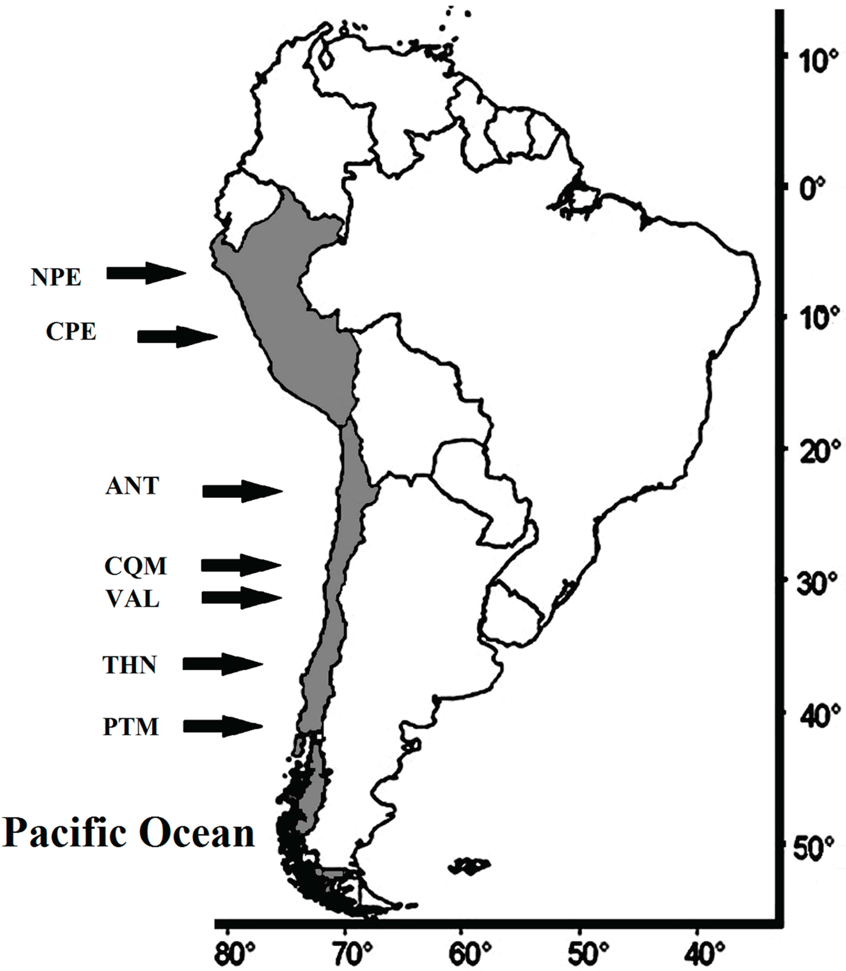
A total of 7142 individuals belonging to three species—E. ringens (n = 2050), T. murphyi (n = 4021) and M. gayi (n = 1071)—were collected from different localities in the SEPO, including two landing ports in Peru—Paita (Northern Peru, NPE), 5° S; and Callao (Central Peru, CPE), 12° S—and five landing ports along the Chilean coast—Antofagasta (ANT); 23°40′ S; Coquimbo (CQM), 30° S; Valparaiso (VAL), 33° S; Talcahuano (THN), 36°40′ S; and Puerto Montt (PTM), 41°30 S—covering a spatial scale of more than 4600 km. The closest landing ports were Coquimbo and Valparaiso, separated by ca. 300 km. (Figure 1). The temporal scale reached a maximum of 24 years, between 1993 and 2017.
In the laboratory, the total length (TL; nearest cm) of the E. ringens and M. gayi and the fork length (FL; nearest cm) of the T. murphyi were measured. Then, the specimens were dissected and examined for metazoan parasites that (as reported previously) affect these species [14,28,31,34]. Specifically, after a necropsy, each fish was carefully examined, first for ectoparasites, in the skin, gills and buccal cavity, and then for endoparasites. All organs, including heart and blood vessels, were examined. To count parasites, each visceral organ was separately dissected and washed in running water. All the material retained in a mesh (0.5 mm) was examined under a stereomicroscope (20x)
Because the parasite communities change through the ontogeny of their fish hosts [26], to avoid the potential effect of host age in the parasite communities a subsample of specimens of similar ages was selected for each host species. To estimate fishes’ ages, the von Bertalanffy growth function was used; the population parameters for E. ringens were K = 0.91, t0 = −0.01 and L∞ = 18.72 [35]; for T. murphyi they were K = 0.16, t0 = −0.13 and L∞ = 75.0 [36]; and for M. gayi they were K = 0.2, t0 = −0.07, and L∞ = 81.9) [37].
2.3. Bibliographic Search
In order to search for references regarding the potential impact of temporal and spatial variability when parasites are used as biological tags, we searched the Web of Science (www.webofknowledge.com, accessed on 8 June 2021) with the following search term: Parasite * stock; Fish * stock identification; fish * stock * discrimination; Parasite * Biological tag. The search was restricted to the years 2000–2020.
2.4. Univariate Analysis
The prevalence and abundance [38] were calculated for each parasite taxon and for each locality and year for each fish species of the same age. To test the hypothesis of an absence of significant differences in the prevalence of each parasite taxon between host species at a spatial scale, samples from the same year were tested (α = 0.05). In a similar way, the hypothesis of an absence of significant differences in the prevalence of each parasite taxon between host species at a temporal scale, samples from the same locality were tested (α = 0.05). Significance in differences in prevalence was tested with Fisher’s exact test [39], and this analysis was performed with R software [40].
Because parasites with a prevalence <5% can be considered accidental [34], only parasite taxa with a prevalence >5% in at least one locality and year were considered in the multivariate analysis.
2.5. Multivariate Analysis
Nonmetric multidimensional scaling (nMDS) was used to graphically visualize patterns of similarity in parasites’ community structures at temporal and spatial scales for each host species. Ordination nMDS plots were constructed from the Bray–Curtis resemblance matrix using abundance values (log n + 1). This analysis was performed on component communities (the mean abundance of each parasite taxon in each fish species) and infra-communities (parasite taxa per individual fish). To evaluate the similarity in parasite communities between localities (spatial) and between years (temporal), we used a permutation-based one-way analysis of similarity (ANOSIM) [41] with the Bray–Curtis index as the similarity measure for abundance data. global R, the statistic for the ANOSIM, ranged from 0 (total similarity) to 1 (total dissimilarity). The statistical significance of the differences between and within sites and years was assessed after 9999 permutations.
The significance of differences between samples from different localities (spatial scale) and years (temporal scale) was tested using a permutational multivariate analysis of variance (PERMANOVA). When differences were detected by the PERMANOVA, pair-wise comparisons allowed us to define which sample (samples) differed.
When significant differences among a priori groups in multivariate space, but not observed in an unconstrained ordination (such as in an MDS plot) [42], a canonical analysis of principal coordinates (CAP) was used as a best alternative [42,43]. To test for significant differences between samples, a permutation trace test (the sum of squared canonical eigenvalues) was applied, and P was obtained after 999 permutations. After the CAP analysis, a correct assignment test was performed [21]. All multivariate analyses (nMDS, ANOSIM, PERMANOVA and CAP) were performed with PRIMER v6 software [44].
3. Results
Of the 7142 individuals belonging to the three host species, a subsample of 3687 individuals were selected, including 1123 E. ringens (12 to 24 months old; range size 11.3–15.7 cm TL), 1904 T. murphyi (24 to 36 months old; range size 21.7–29.5 cm FL) and 630 M. gayi (36 to 48 months old; range 37.3–45.6 cm TL). The number of hosts collected in each locality and year are indicated in the supplementary material (the sheet Samples).
A total of 9 parasite taxa were found in E. ringens, 15 in T. murphyi and 23 in M. gayi. The complete list of parasites found in each host species is given in the supplementary material (the sheet Parasites). Prevalences greater than 5% were observed in: 7 taxa (2 at the larval stage and 5 adults) for E. ringens; 13 taxa (6 at the larval stage and 7 adults) for T. murphyi; and 17 taxa (7 larval stage and 10 adults) for M. gayi. The remaining taxa were removed from subsequent analyses. The values of prevalence for each parasite species found in each host species (within subsamples of the same age) and locality are shown in the supplementary material (the sheet Prevalence).
3.1. Spatial Analysis
For the three host species, most of the parasite taxa showed differences in prevalence at a spatial scale for the same year. Bothriocephalus sp. in E. ringens did not show differences at the spatial scale, and Pseudanthocotyloides heterocotyle and Anisakis sp. showed differences between localities in 2007 and 2016. Ceratothoa gaudichaudi in T. murphyi did not show differences between localities in 1993, 2008 and 2012. Six parasite taxa—Corynosoma sp. and Caligus bonito (for 1993); Rhadinorhynchus trachuri Anisakis sp. and Lernanthropinus trachuri (for 2008); and Hysterothylacium sp. (for 2011)—did not show differences at the spatial scale. All parasites of M. gayi except two (Corynosoma sp. and Anisakidae gen. sp.) showed differences between localities, and three (Parabrachiella insidiosa, Anthocotyle merluccii and Rhadinorhynchus sp.) showed differences only in one year; see the supplementary material (the sheet Spatial analysis).
The ANOSIM showed significant differences in the parasite communities for different localities among the three species. For E. ringens (global R = 0.054; p < 0.001) and T. murphyi (global R = 0.141; p < 0.001), the pairwise test was significant for all pairs of comparisons. For M. gayi (global R = 0.052; p < 0.05), the pairwise test was significant for all pairs of comparisons except CQM–VAL (R = −0.023; p = 0.870), CQM–THN (R = 0.009; p = 0.275) and VAL–THN (R = 0.007; p = 0.168). PERMANOVA showed significant differences in the parasite communities from different localities in the three host species. For E. ringens (pseudo-F = 39.491; p < 0.0001) for T. murphyi (pseudo-F = 103.45; p = 0.001) and M. gayi (pseudo-F = 18.963); p < 0.0001). Pairwise tests were significant for all pairs of comparisons.
In general, across the three host species, the CAP analysis showed significant differences between parasite communities at the spatial scale in the same year. Differences were observed in all cases for E. ringens; samples for 1995, 2005 and 2007 showed lower values of correct assignation (CA), at close to 50%, but in 2006 and 2016 the values of CA were higher than 65%. In all cases, values of assignation due to chance (AdC) were lower than those of CA. For T. murphyi, differences were evident for three of the five samples; the values of CA were lower, close to 50% (except in 2012 = 96.8%), and the values of AdC in all cases were lower than those of CA except in 1993. For M. gayi, significant differences were observed in both samples, the values of CA were lower (<55%) and the values of AdC were lower than those of CA.
The values of the CAP analysis and percentages of CA and AdC for the spatial analysis are shown in the supplementary material (the sheet Correct allocation).
3.2. Temporal Analysis
The prevalence of Anisakis sp. (ANT and CQM), P. heterocotyle (CQM), Bothriocephalus sp. (THN) and Caligus sp. (ANT) in E. ringens did not show significant differences at the temporal scale. The prevalence of Scolex pleuronectis (ANT), Nybelinia surmenicola, Corynosoma australe, C. bonito, Ceratothoa gaudichaudi (CQM) and Pseudoterranova sp. (THN) in T. murphyi did not show significant differences at the temporal scale. The prevalence of Corynosoma sp. (CQM, VAL and THN); P. insidiosa Anisakidae gen sp. (VAL, THN and PTM) and Clestobothrium crassiceps (VAL and PTM); Hepatoxylon trichiuri (THN); R. trachuri (CQM); and Chondracanthus australis (CQM) in M. gayi did not show significant differences at the temporal scale. The values of Fisher’s exact test for each parasite taxon between years are shown in the supplementary material (the sheet Temporal analysis).
For the three host species, the ANOSIM showed significant differences in the parasite communities at the temporal scale. For E. ringens (global R = 0.124; p < 0.001), the pairwise test was significant for all pairs of years except 1995/2007 (R = −0.088; p > 0.05) and 2005/2007 (R −0.041 = p > 0.05). For T. murphyi (global R = 0.126; p < 0.001), the pairwise test was significant for all pairs of years except 2005/1993 (R = −0.047; p > 0.05), 2006/1993 (R = 0.006; p > 0.05) and 2008/2011 (R = −0.002; p > 0.05). Finally, for M. gayi (global R = 0.166; p < 0.001), the pairwise test was significant for all pairs of years except 1995/2017 (R = 0.00; p = 0.465), 2005/2017 (R = 0.032; p = 0.353) and 2006/2017 (R = −0.094; p = 0.781). The PERMANOVA showed significant differences in the parasite communities for different years: for E. ringens, pseudo-F = 65.609 (p < 0.0001); for T. murphyi, pseudo-F = 83.054; and for M. gayi, pseudo-F = 15.861 (p ≤ 0.0001). Pairwise tests showed significant differences for all pairs of comparison across the three host species.
For the three host species, the CAP analysis showed significant differences between parasite communities at the temporal scale for the same locality. For E. ringens, the values of CA were lower, close to 50%, and the values of AdC were lower than those of CA in all cases. In T. murphyi, the values of CA were lower, close to 50%, except for THN (98%), and the values of AdC were lower than those of CA in three of the five comparisons. M. gayi showed significant differences in all cases: the values of CA were high (>69%) and the values of AdC were lower than those of CA in all cases. The values of the CAP and the percentages of CA and AdC in the temporal analysis are shown in the supplementary material (the sheet Correct allocation).
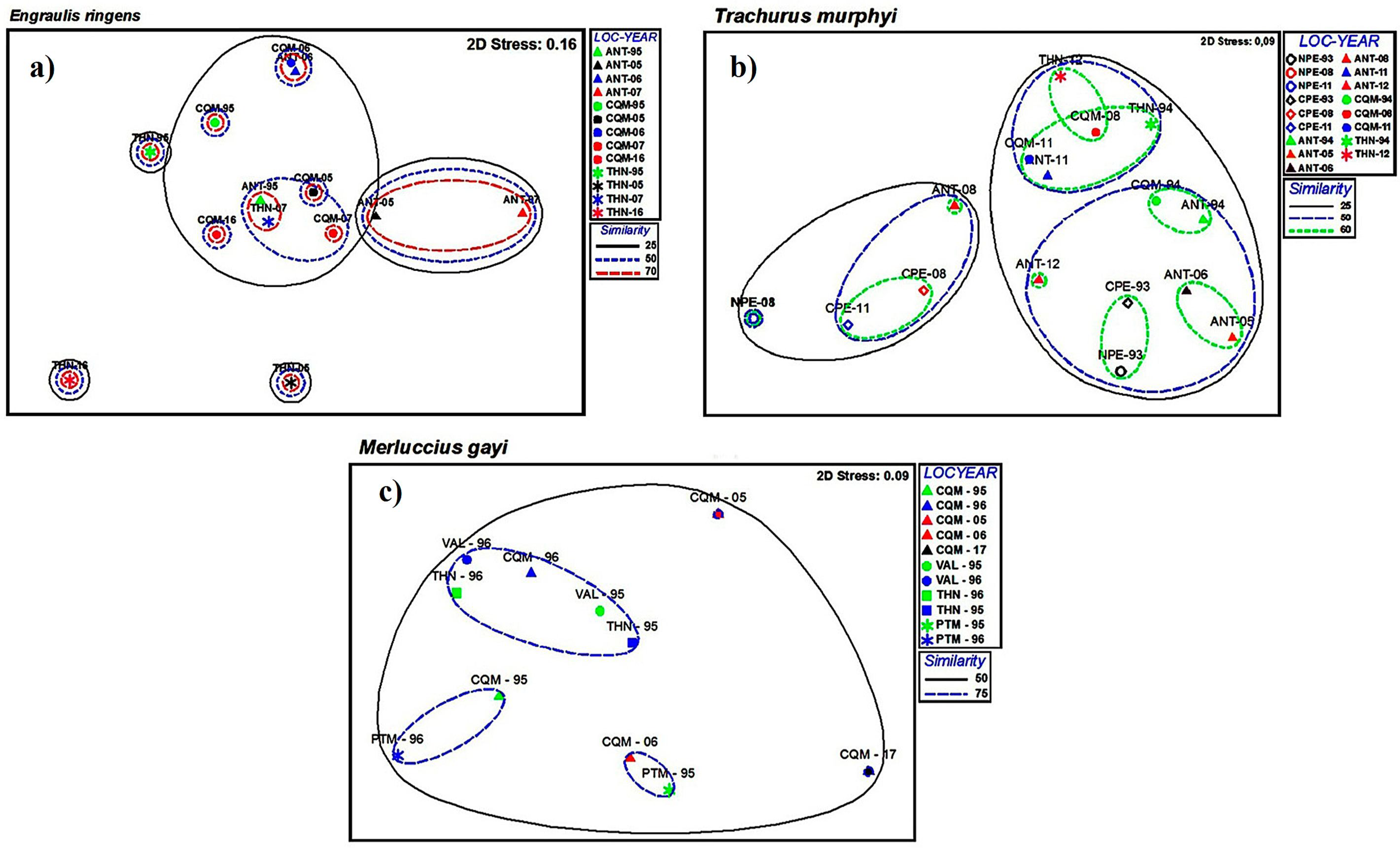
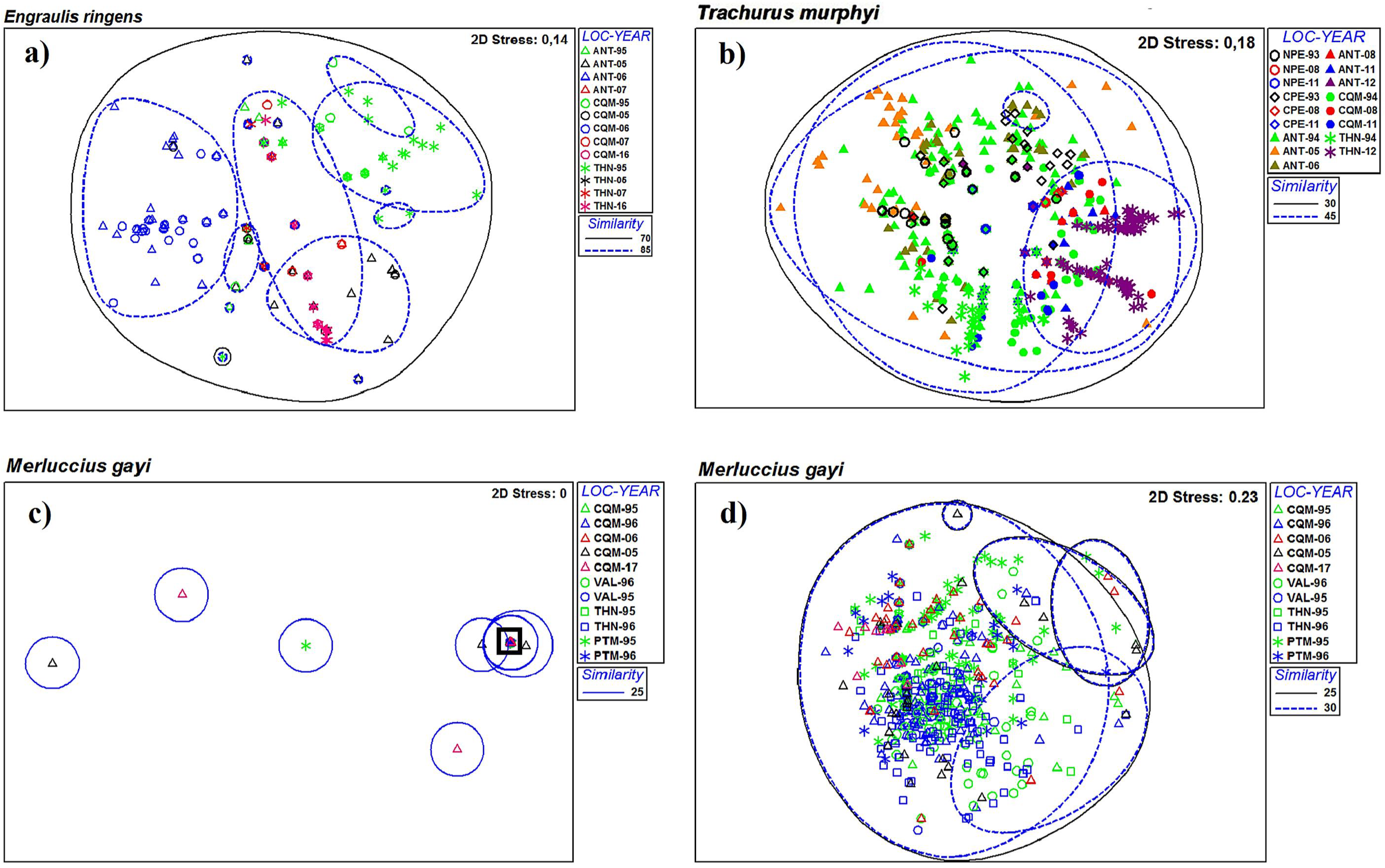
The bi-dimensional graphic representation (nMDS) of the parasitic component communities for each host species at the same locality but in different years is shown in Figure 2. The graphic for E. ringens suggests that closer localities (exceptions: THN-05, THN-16) showed higher similarities than farther localities. For T. murphyi, three major groups showed similarities at 50% but without a clear spatial or temporal pattern. A different scenario occurred for M. gayi, with high values of similarity between all samples except for CQM-05 and CQM-17. The same graphic analysis for infra-communities showed similarities over 50% for all spatiotemporal samples of E. ringens, but T. murphyi and M. gayi did not show evident temporal/spatial patterns. For M. gayi, most of the data overlap and a subset (black square) was performed for better visualization (Figure 3).
4. Discussion
One way to mitigate uncertainty about the sustainability of global fisheries is to achieve precise assessments of the abundance of resources in space and time and collect information on stock structures as a first step [4]. For almost a century, parasites have been successfully used in fish stock identification [5,6]. Currently, parasites are considered an appropriate tool in fisheries management, specifically as BTs for stock identification [4]. When using parasites as BTs for fish stock identification, it is desirable to know the age of host individuals [12]. Although, for some species, an age determination has not been validated [12], most studies have used the lengths of fishes to compare groups of fishes from different localities [45,46]. Of 102 published articles using fish parasites as BTs in the last 20 years, for 66 the goal was stock identification, but host age (or ontogeny stage) was considered in only 14. Fishes of similar length could include individuals of different ages that therefore would have been exposed to parasite infections for different periods, generating a confounding factor in the interpretation of results, specifically for parasites at the larval stage, because these parasites accumulate over time [26].
The utility of parasites as BTs for stock identification is determined to an extent by the temporal stability of the parasite communities, particularly when different localities have been sampled across different seasons or years [47]. However, in this kind of study, spatiotemporal variability in parasite communities has been poorly evaluated.
Of the 102 studies published from 2000 to 2020, 38 included samples from 2 or more years and 12 compared samples from different years; however, the samples were pooled, because the temporal variability in each sample locality was not measured. The variability at the temporal and/or spatial scales was analyzed in only nine studies. Samples of Clupea harengus collected between 2002 and 2005 and compared with samples obtained in 1973 and 1982 suggested that parasite fauna are spatially variable but remain temporally stable over the short and long term [48]. Samples of Mullus surmuletus in three localities and two seasons in different years, showed that due to the high small-scale variability (across samples from the same localities), it was not possible to identify different stocks [24]. For Pinguipes brasilianus collected in different seasons between 2006 and 2007 [25], the spatial effects exceeded seasonal effects. Similarly, an analysis of parasite communities in Percophis brasiliensis, conducted across seasons over one year, showed that parasite communities in seasonal samples had a high degree of homogeneity in infection levels within and between samples throughout the year [15]; therefore, parasites can be used for fish stock identification independent of the season of capture, at least on an annual scale. Parasite communities of Polydactylus macrochir from different periods between 2007 and 2009 showed stability over the temporal scale explored [49]. Temporal variability but marked spatial differences in the infection of metacercaria supported the hypothesis regarding two stocks of Sardinops sagax [50]. Among studies that evaluated possible spatial and/or temporal variability in parasite communities by comparing samples from temporal scales in the same locality, Moore [51] analyzed the parasites of Scyliorhinus canicula, including samples from three localities; however, because samples taken over different periods from the same locality were small, samples from each locality were grouped and analyzed as a single sample. The local variability in the parasites of E. ringens studied through five subsamples (n = 60 c/u) from two localities less than 60 km apart and collected within two days of separation to avoid potential temporal noise showed that variability could be well represented with a single sample [14]; but in the same species, the magnitude of local variation was higher than regional variability; therefore, the effect of high local variability must be considered [16].
4.1. Spatial Variability
The spatial variability of parasite communities allows the use of parasites as biological tags for fish stock identification [15], because a parasite species is found only in those areas where conditions are suitable for its transmission [12]. A parasite must have specific features to be considered as a BT, parasite taxa must present significant differences in prevalence or load across the study area [12]. For the three host species, most of the parasite taxa showed differences in prevalence at the spatial scale for a given time. In E. ringens, only Botriocephalus sp. showed similar prevalences in all localities, and the remaining parasite taxa showed differences between localities at least on time. In T. murphyi and M. gayi, all parasite taxa showed differences at the spatial scale, but with two exceptions in M. gayi (Corynosoma sp. and Anisakidae gen. sp.). The ANOSIM showed differences in parasite communities between localities in E. ringens and T. murphyi but not M. gayi; nevertheless, the PERMANOVA and CAP showed that significant differences between communities were detected in the three species.
The CAP analysis showed significant differences between communities (with exceptions) and the values of CA were low. The low values of CA could be explained by samples of one locality being assigned to a nearby locality. For example, in E. ringens 1995, total CA = 55.8% (ANT = 96.6%; CQM = 0%; THN = 50%), but 56 of 68 samples from CQM were allocated to ANT. In T. murphyi 2011, total CA = 55.6% (ANT = 34.0%; CQM = 50.9; NPE = 0; CEP = 97.5), but 67 of 69 samples from NPE were allocated to CPE. In M. gayi, the highest values of CA were allocated to the most geographically distant localities (CQM and PTM). Therefore, although the spatial variability was lower, the communities were well assigned to their hosts’ localities of origin or to the nearest locality. These results could be due to specimens belonging to the same stock sharing similar parasite communities but landing in different but closer ports or due to each locality representing a landing port but fishing areas of closer ports overlapping [34].
4.2. Temporal Variability
Comparative studies over long periods require a high degree of temporal repetition in the composition and structure of parasite communities [25], the only way to avoid the potential impact of temporal variability on the structure of parasite communities. Although studies that have analyzed the variability in parasite communities at different temporal scales exist, long-term comparisons are rare [48]. Analyzing long-term samples, most parasite taxa (at the same locality) present different prevalence rates between years, although some taxa (Anisakis sp. from E. ringens; N. surmenicola, Pseudoterranova sp. from T. murphyi; and P. insidiosa, C. australis, C. crassiceps H. trichiuri, Rhadinorhynchus sp., Corynosoma sp. and Anisakidae gen. sp. from M. gayi) remained constant throughout different years. Many of these taxa (six) were in the larval stage, and it has been stated that these long-lived parasites confer temporal stability to community parasites at least at the seasonal or annual scale [52]. Our results support desirable long-term temporal stability as a prerequisite for the use of parasites as BTs [12] but for fishes of the same age or the same cohort.
5. Conclusions
In conclusion, for comparative studies over long periods, a high degree of temporal repeatability is required, as suggested previously [15], but in a scenario with temporal variability, caution must be taken when using samples from different years from a given locality. Nevertheless, in a scenario with temporal stability samples from the same locality but different years can be pooled. On the other hand, as suggested recently [26], older hosts harbors relatively more stable parasite communities; consequently, older age classes present in a given sample are preferable when using parasites as BTs.
Supplementary Materials
The following supplementary material is available online at https://0-www-mdpi-com.brum.beds.ac.uk/article/10.3390/fishes6040071/s1, Espinola-Novelo and Oliva.xlsx.
Author Contributions
Conceptualization, J.F.E.-N. and M.E.O.; methodology, J.F.E.-N. and M.E.O.; validation, M.E.O.; formal analysis, J.F.E.-N.; investigation, J.F.E.-N. and M.E.O.; resources, M.E.O.; data curation, J.F.E.-N. and M.E.O.; writing—original draft preparation, J.F.E.-N.; writing—review and editing, J.F.E.-N. and M.E.O.; supervision, M.E.O. All authors have read and agreed to the published version of the manuscript.
Funding
This research received no external funding.
Institutional Review Board Statement
This study was approved by the Ethical Commission of the Universidad de Antofagasta, Antofagasta, Chile. This study did not consider experiments with live animals. All fishes were obtained from commercial catches and none of the species are subject to conservation measures. Commercial fishermen follow national regulations concerning these fisheries.
Data Availability Statement
Data is available in the Supplementary Material.
Conflicts of Interest
The authors declare no conflict of interest.
References
- Cadrin, S.X. Defining spatial structure for fishery stock assessment. Fish. Res. 2020, 221, 105397. [Google Scholar] [CrossRef]
- Cadrin, S.X.; Friedland, K.D.; Waldman, J.R. Stock identification methods: An Overview. In Stock Identification Methods: Applications in Fishery Science, 1st ed.; Cadrin, S.X., Friedland, K.D., Waldman, J.R., Eds.; Elsevier Academic Press: Amsterdam, The Netherlands, 2005; pp. 2–6. [Google Scholar]
- Sparre, P.; Venema, C.S. Introduction to Tropical Fish Stock Assessment. Part I: Manual; FAO: Rome, Italy, 1998; p. 407. [Google Scholar]
- Timi, J.T.; MacKenzie, K. Parasites in fisheries and mariculture. Parasitology 2015, 142, 1–4. [Google Scholar] [CrossRef] [PubMed] [Green Version]
- Herrington, W.C.; Bearse, H.M.; Firth, F.E. Observations on the life history, occurrence and distribution of the redfish parasite Sphyrion lumpi; United States Department of the Interior, Bureau of Fisheries: Washington, DC, USA, 1939; Volume 5, pp. 1–18. [Google Scholar]
- Dogiel, V.A.; Bychovsky, B.E. Parasites of the fishes of the Caspian Sea. Tr. Kompleks. Izucheniyu Kaspiikogo Morya 1939, 7, 1–150. [Google Scholar]
- Canel, D.; Levya, E.; Soares, I.A.; Braicovich, P.E.; Haimovicic, M.; Luque, J.L.; Timi, J.T. Stocks and migrations of the demersal fish Umbrina canosai (Sciaenidae) endemic from the subtropical and temperate Southwestern Atlantic revealed by its parasites. Fish. Res. 2019, 214, 10–18. [Google Scholar] [CrossRef]
- Hermida, M.; Cavaleiro, B.; Gouveia, L.; Saraiva, A. Seasonality of skipjack tuna parasites in the Eastern Atlantic provide an insight into its migratory patterns. Fish. Res. 2019, 216, 167–173. [Google Scholar] [CrossRef]
- Boudaya, L.; Feki, M.; Mosbahi, N.; Neifar, L. Stock discrimination of Chelidonichthys obscurus Triglidae in the central Mediterranean Sea using morphometric analysis and parasite markers. J. Helminthol. 2020, 94, E74. [Google Scholar] [CrossRef] [PubMed]
- Mackenzie, K. Parasites as biological tags in population studies of marine organisms: An update. Parasitology 2002, 124, 153–163. [Google Scholar] [CrossRef] [PubMed]
- Braicovich, P.E.; Ieno, E.N.; Sáez, M.; Despos, J.; Timi, J.T. Assessing the role of host traits as drivers of the abundance of long-lived parasites in fish-stock assessment studies. J. Fish Biol. 2016, 89, 2419–2433. [Google Scholar] [CrossRef] [PubMed]
- MacKenzie, K.; Abaunza, P. Parasites as Biological Tags. In Stock Identification Methods: Applications in Fishery Science, 2nd ed.; Cadrin, S.X., Kerr, L.A., Mariani, S., Eds.; Elsevier Academic Press: Burlington, MA, USA, 2014; pp. 185–203. [Google Scholar] [CrossRef]
- Pascual, S.; Abollo, E.; González, A.F. Biobanking and genetic markers for parasites in fish stock studies. Fish. Res. 2016, 173, 214–220. [Google Scholar] [CrossRef]
- Chavez, R.A.; Valdivia, I.M.; Oliva, M.E. Local variability in metazoan parasites of the pelagic fish species, Engraulis ringens: Implications for fish stock assessment using parasites as biological tags. J. Helminthol. 2007, 81, 113–116. [Google Scholar] [CrossRef] [PubMed]
- Braicovich, P.E.; Timi, J.T. Seasonal stability in parasite assemblages of the Brazilian flathead, Percophis brasiliensis (Perciformes: Percophidae): Predictable tools for stock identification. Folia Parasitol. 2010, 57, 206–212. [Google Scholar] [CrossRef] [PubMed] [Green Version]
- George-Nascimento, M.; Moscoso, D. Variación local y geográfica de las infracomunidades de parásitos de la anchoveta Engraulis ringens en Chile. Rev. Biol. Mar. Oceanogr. 2013, 48, 207–212. [Google Scholar] [CrossRef] [Green Version]
- Levy, E.; Canel, D.; Rossin, M.A.; Hernández-Orts, J.S.; González-Castro, M.; Timi, J.T. Parasites as indicators of fish population structure at two different geographical scales in contrasting coastal environments of the south-western Atlantic. Estuar. Coast. Shelf Sci. 2019, 229, 106400. [Google Scholar] [CrossRef]
- Charters, R.A.; Lester, R.J.G.; Buckworth, R.C.; Newman, S.J.; Ovendend, J.R.; Broderick, D.; Kravchuke, O.; Ballaghf, A.; Welchfg, D.J. The stock structure of grey mackerel Scomberomorus semifasciatus in Australia as inferred from its parasite fauna. Fish. Res. 2010, 101, 94–99. [Google Scholar] [CrossRef]
- Lester, R.J.G.; MacKenzie, K. The use and abuse of parasites as stock markers for fish. Fish. Res. 2009, 97, 1–2. [Google Scholar] [CrossRef]
- Connell, J.H.; Sousa, W.P. On the evidence needed to judge ecological stability or persistence. Am. Nat. 1983, 121, 789–824. [Google Scholar] [CrossRef]
- Poulin, R.; Kamiya, T. Parasites as biological tags of fish stocks: A meta-analysis of their discriminatory power. Parasitology 2015, 142, 145–155. [Google Scholar] [CrossRef]
- Bennett, S.N.; Adamson, M.L.; Margolis, L. Long-term changes in parasites of sockeye salmon (Oncorhynchus nerka) smolts. Can. J. Fish. Aquat. Sci. 1998, 55, 977–986. [Google Scholar] [CrossRef]
- Grutter, A.S. Spatial and temporal variations of the ectoparasites of seven reef fish species from Lizard Island and Heron Island, Australia. Mar. Ecol. Prog. Ser. 1994, 115, 21–30. [Google Scholar] [CrossRef]
- Ferrer-Castelló, E.; Raga, J.A.; Aznar, F.J. Parasites as fish population tags and pseudoreplication problems: The case of striped red mullet Mullus surmuletus in the Spanish Mediterranean. J. Helminthol. 2007, 81, 169–178. [Google Scholar] [CrossRef]
- Timi, J.T.; Lanfranchi, A.L.; Etchegoin, J.A. Seasonal stability and spatial variability of parasites in Brazilian sandperch Pinguipes brasilianus from the Northern Argentine Sea: Evidence for stock discrimination. J. Fish Biol. 2009, 74, 1206–1225. [Google Scholar] [CrossRef] [PubMed]
- Espínola-Novelo, J.F.; González, M.T.; Pacheco, A.S.; Luque, J.L.; Oliva, M.E. Testing for deterministic succession in metazoan parasite communities of marine fish. Ecol. Lett. 2020, 23, 631–641. [Google Scholar] [CrossRef]
- George-Nascimento, M.; Oliva, M.E. Fish population studies using parasites from the Southeastern Pacific Ocean: Considering host population changes and species body size as sources of variability of parasite communities. Parasitology 2015, 142, 25–35. [Google Scholar] [CrossRef] [PubMed]
- Valdivia, I.M.; Chávez, R.A.; Oliva, M.E. Metazoan parasites of Engraulis ringens as tools for stock discrimination along the Chilean coast. J. Fish Biol. 2007, 70, 1504–1511. [Google Scholar] [CrossRef]
- George-Nascimento, M.; Arancibia, H. Stocks ecológicos del jurel (Trachurus symmetricus murphyi Nichols) en tres zonas de pesca frente a Chile, detectados mediante comparación de su fauna parasitaria y morfometría. Rev. Chil. Hist. Nat. 1992, 65, 453–470. [Google Scholar]
- Aldana, M.; Oyarzún, J.; George-Nascimento, M. Isópodos parásitos como indicadores poblacionales del jurel Trachurus symmetricus murphyi (Nichols, 1920) (Pisces: Carangidae) frente a las costas de Chile. Biol. Pesq. 1995, 24, 23–32. [Google Scholar]
- Oliva, M.E. Metazoan parasites of the jack mackerel Trachurus murphyi (Teleostei, Carangidae) in a latitudinal gradient from South America (Chile and Peru). Parasite 1999, 6, 223–230. [Google Scholar] [CrossRef] [PubMed] [Green Version]
- George-Nascimento, M. Geographical variations in the jack mackerel Trachurus symmetricus murphyi populations in the southeastern Pacific Ocean as evidenced from the associated parasite communities. J. Parasitol. 2000, 86, 929–932. [Google Scholar] [CrossRef]
- George-Nascimento, M. Populations and assemblages of parasites in hake, Merluccius gayi, from the southeastern Pacific Ocean: Stock implications. J. Fish Biol. 1996, 48, 557–568. [Google Scholar] [CrossRef]
- Oliva, M.E.; Ballón, I. Metazoan parasites of the Chilean hake Merluccius gayi gayi as a tool for stock discrimination. Fish. Res. 2002, 56, 313–320. [Google Scholar] [CrossRef]
- Canales, M.T.; Leal, E. Parámetros de historia de vida de la anchoveta Engraulis ringens Jenyns, 1842, en la zona centro norte de Chile. Rev. Biol. Mar. Oceanogr. 2009, 44, 173–179. [Google Scholar] [CrossRef] [Green Version]
- Cisterna, L.; Arancibia, H. Age of Jack mackerel Trachrus murphyi (Carangidae) using daily growth rings in sagittae otoliths. Gayana 2017, 81, 28–31. [Google Scholar] [CrossRef] [Green Version]
- Froese, R.; Pauly, D. World Wide Web Electronic Publication. Fishbase. 2021. Available online: www.fishbase.org (accessed on 4 August 2021).
- Bush, A.O.; Lafferty, K.D.; Lotz, J.M.; Shostak, A.W. Parasitology meets ecology on its own terms: Margolis et al. revisited. J. Parasitol. 1997, 83, 575–583. [Google Scholar] [CrossRef] [PubMed]
- Reiczigel, J.; Marozzi, M.; Fábián, I.; Rózsa, L. Biostatistics for Parasitologists—A Primer to Quantitative Parasitology. Trends Parasitol. 2019, 35, 277–281. [Google Scholar] [CrossRef]
- R Core Team. R: A Language and Environment for Statistical Computing; R Foundation for Statistical Computing: Vienna, Austria, 2019; Available online: https://www.R-project.org/ (accessed on 17 January 2020).
- Clarke, K.R. Non-parametric multivariate analyses of changes in community structure. Aust. J. Ecol. 1993, 18, 117–143. [Google Scholar] [CrossRef]
- Anderson, M.J.; Gorley, R.N.; Clarke, K.R. PERMANOVA+ for PRIMER: Guide to Software and Statistical Methods; Primer-E: Plymouth, UK, 2008. [Google Scholar]
- Anderson, M.J.; Willis, T.J. Canonical analysis of principal coordinates: A useful method of constrained ordination for ecology. Ecology 2003, 84, 511–525. [Google Scholar] [CrossRef]
- Clarke, K.R.; Gorley, R.N. Primer V6: User Manual/Tutorial; Primer-E: Plymouth, UK, 2006. [Google Scholar]
- Braicovich, P.E.; Timi, J.T. Parasites as biological tags for stock discrimination of the Brazilian flathead Percophis brasiliensis in the south-west Atlantic. J. Fish Biol. 2008, 73, 557–571. [Google Scholar] [CrossRef]
- Bottari, T.; Gaglio, G.; Mobilia, V.; Garofalos, G.; Laria, C.; Fiorentino, F. Discrimination of Red Mullet Populations (Teleostean, Mullidae) Off the Sicilian Coasts (Mediterranean Sea) on the Basis of Metazoan Parasites. Thalassas 2000, 6, 357–363. [Google Scholar] [CrossRef]
- Moore, B.R.; Stapley, J.; Allsop, Q.; Newman, S.J.; Ballagh, A.; Welch, D.J.; Lester, R.J.G. Stock structure of blue threadfin Eleutheronema tetradactylum across northern Australia, as indicated by parasites. J. Fish Biol. 2011, 78, 923–936. [Google Scholar] [CrossRef]
- Campbell, N.; Cross, M.A.; Chubb, J.C.; Cunningham, C.O.; Hatfield, E.M.C.; MacKenzie, K. Spatial and temporal variations in parasite prevalence and infracommunity structure in herring (Clupea harengus L.) caught to the west of the British Isles and in the North and Baltic Seas: Implications for fisheries science. J. Helminthol. 2007, 81, 137–146. [Google Scholar] [CrossRef]
- Moore, B.R.; Welch, D.J.; Newman, S.J.; Lester, R.J.G. Parasites as indicators of movement and population connectivity of a non-diadromous, tropical estuarine teleost: King threadfin Polydactylus macrochir. J. Fish Biol. 2012, 81, 230–252. [Google Scholar] [CrossRef] [PubMed]
- Weston, L.F.; Reed, C.C.; Hendricks, M.; Winker, H.; van der Lingen, C.D. Stock discrimination of South African sardine (Sardinops sagax) using a digenean parasite biological tag. Fish. Res. 2015, 164, 120–129. [Google Scholar] [CrossRef]
- Moore, A.B.M. Metazoan parasites of the lesser-spotted dogfish Scyliorhinus canicula and their potential as stock discrimination tools. J. Mar. Biol. Assoc. UK 2001, 81, 1009–1013. [Google Scholar] [CrossRef] [Green Version]
- Cantatore, D.M.P.; Timi, J.T. Marine parasites as biological tags in South American Atlantic waters, current status and perspectives. Parasitology 2015, 142, 5–24. [Google Scholar] [CrossRef] [PubMed] [Green Version]
Figure 1.
Approximate position of sampling localities. NPE = Paita 5° S (Northern Peru); CPE = Callao 12° S (Central Peru); ANT = Antofagasta 23°40′ S (Chile); CQM = Coquimbo 30° S (Chile); VAL = Valparaiso 33° S (Chile); THN = Talcahuano 36°40′ S (Chile); PTM = Puerto Montt 41°30′ S (Chile).
Figure 1.
Approximate position of sampling localities. NPE = Paita 5° S (Northern Peru); CPE = Callao 12° S (Central Peru); ANT = Antofagasta 23°40′ S (Chile); CQM = Coquimbo 30° S (Chile); VAL = Valparaiso 33° S (Chile); THN = Talcahuano 36°40′ S (Chile); PTM = Puerto Montt 41°30′ S (Chile).

Figure 2.
Non-metric multidimensional scaling (nMDS) of parasite communities in three fish species in the southeastern Pacific Ocean: (a) E. ringens; (b), T. murphyi; (c), Merluccius gayi. Circles represent similarity levels between samples of locality–year.
Figure 2.
Non-metric multidimensional scaling (nMDS) of parasite communities in three fish species in the southeastern Pacific Ocean: (a) E. ringens; (b), T. murphyi; (c), Merluccius gayi. Circles represent similarity levels between samples of locality–year.

Figure 3.
Non-metric multidimensional scaling (nMDS) of parasite infra-communities in three fish species in the southeastern Pacific Ocean: (a), Engraulis ringens; (b), Trachurus murphyi; (c), Merluccius gayi; (d), subset (of the black square) of Merluccius gayi in (c). Circles represent similarity levels between samples of locality–year.

Publisher’s Note: MDPI stays neutral with regard to jurisdictional claims in published maps and institutional affiliations. |
© 2021 by the authors. Licensee MDPI, Basel, Switzerland. This article is an open access article distributed under the terms and conditions of the Creative Commons Attribution (CC BY) license (https://creativecommons.org/licenses/by/4.0/).
Share and Cite
MDPI and ACS Style
Espínola-Novelo, J.F.; Oliva, M.E. Spatial and Temporal Variability of Parasite Communities: Implications for Fish Stock Identification. Fishes 2021, 6, 71. https://0-doi-org.brum.beds.ac.uk/10.3390/fishes6040071
AMA Style
Espínola-Novelo JF, Oliva ME. Spatial and Temporal Variability of Parasite Communities: Implications for Fish Stock Identification. Fishes. 2021; 6(4):71. https://0-doi-org.brum.beds.ac.uk/10.3390/fishes6040071
Chicago/Turabian StyleEspínola-Novelo, Juan F., and Marcelo E. Oliva. 2021. "Spatial and Temporal Variability of Parasite Communities: Implications for Fish Stock Identification" Fishes 6, no. 4: 71. https://0-doi-org.brum.beds.ac.uk/10.3390/fishes6040071