Topological Edge States of a Majorana BBH Model

Abstract

We investigate a Majorana Benalcazar–Bernevig–Hughes (BBH) model showing the emergence of topological corner states. The model, consisting of a two-dimensional Su–Schrieffer–Heeger (SSH) system of Majorana fermions with $\pi$ flux, exhibits a non-trivial topological phase in the absence of Berry curvature, while the Berry connection leads to a non-trivial topology. Indeed, the system belongs to the class of second-order topological superconductors ($HOTS{C}_2$), exhibiting corner Majorana states protected by $C_4$ symmetry and reflection symmetries. By calculating the 2D Zak phase, we derive the topological phase diagram of the system and demonstrate the bulk-edge correspondence. Finally, we analyze the finite size scaling behavior of the topological properties. Our results can serve to design new $2D$ materials with non-zero Zak phase and robust edge states.

1. Introduction

The notion of higher order topological phases first appeared for insulating systems ($HOTIs$) [1,2,3,4]. Indeed, a second-order topological insulator is a d dimensional system with gapped $d-1$ dimensional boundaries and $d-2$ localized modes (corner states in two-dimensional systems). This new topological phase can be protected by a variety of crystalline symmetries, such as reflection symmetries and $C_4$ symmetry [1].

Recently, a similar physics has also been explored in the context of superconducting systems ($HOTSCs$) [5,6,7,8,9]. Superconductors with such novel topological properties have attracted increasing attention as they possess surface states that propagate along one-dimensional curves (hinges) or are localized at some points (corners) on the surface. In particular, m-dimensional Majorana corner states can be realized in d-dimensional superconductors, with $m\le d-2$.

In close analogy with Ref. [2], we consider a Benalcazar–Bernevig–Hughes (BBH) model of Majorana fermions and will show that it is a suitable model to realize an $HOTSC$ with robust corner Majorana zero modes. It has been demonstrated that the original fermionic $2D$ SSH model cannot support topological corner states [10,11] unless one considers a negative coupling per plaquette, as theoretically proposed [2] and experimentally demonstrated in [12,13,14]. On the other hand, in our model, the mapping of Majorana fermions onto complex fermion operators gives rise to a model of Kitaev chains coupled by a staggered pairing coupling, showing a higher order topological phase. Despite being characterized by a specific set of parameters, our model could be realized in photonics systems where a high efficiency to control parameters through gauge fields has been demonstrated [15,16]. Furthermore, our model could have several interesting and potential applications, in particular, in studying the braiding dynamics of Majorana fermions [17] for condensed matter platforms. Topological insulators are phases of matter characterized by topological edge states that propagate in a unidirectional manner that is robust to imperfections and disorder. They propose a concept that exploits topological effects in a unique way: the topological insulator laser. These are lasers whose lasing mode exhibits topologically protected transport without magnetic fields. The underlying topological properties lead to a highly efficient laser, robust to defects and disorder, with single-mode lasing even at very high gain values. The topological insulator laser alters current understanding of the interplay between disorder and lasing, and at the same time, opens exciting possibilities in topological physics, such as topologically protected transport in systems with gain. On the technological side, the topological insulator laser provides a route to arrays of semiconductor lasers that operate as one single-mode high-power laser coupled efficiently into an output port.

The paper is thus organized as follows. In Section 2, we present the model and the lattice geometry. In Section 3, we discuss the phase diagram and check the bulk-edge correspondence. Section 4 is devoted to the analysis of the finite size scaling of the topological properties. In particular, we discuss the behavior of the gaps closing and the non-local fermion correlation functions. Conclusions are drawn in Section 5. Appendix A contains details on the calculation of non-local fermion correlations.

2. Model

We consider a two dimensional lattice model of Majorana fermions with staggered couplings $w,v$ which define a plaquette with $\pi$ flux, (see Figure 1, panel (a)) described by the Hamiltonian:

$$\begin{array}{c}\hfill \begin{array}{cc}\hfill H=& \frac{i}{2}[w\sum _{m,l=1}^{L,N}{a}_{m,l}{b}_{m,l}+v\sum _{m,l=1}^{L-1,N}{b}_{m,l}{a}_{m+1,l}+w\sum _{l=1}^{N-1,2}\sum _{m=1}^L\left(b_{m,l}{b}_{m,l+1}-a_{m,l}{a}_{m,l+1}\right)\hfill \\ & +v\sum _{l=2}^{N-1,2}\sum _{m=1}^L\left(b_{m,l}{b}_{m,l+1}-a_{m,l}{a}_{m,l+1}\right)],\hfill \end{array}\end{array}$$

(1)

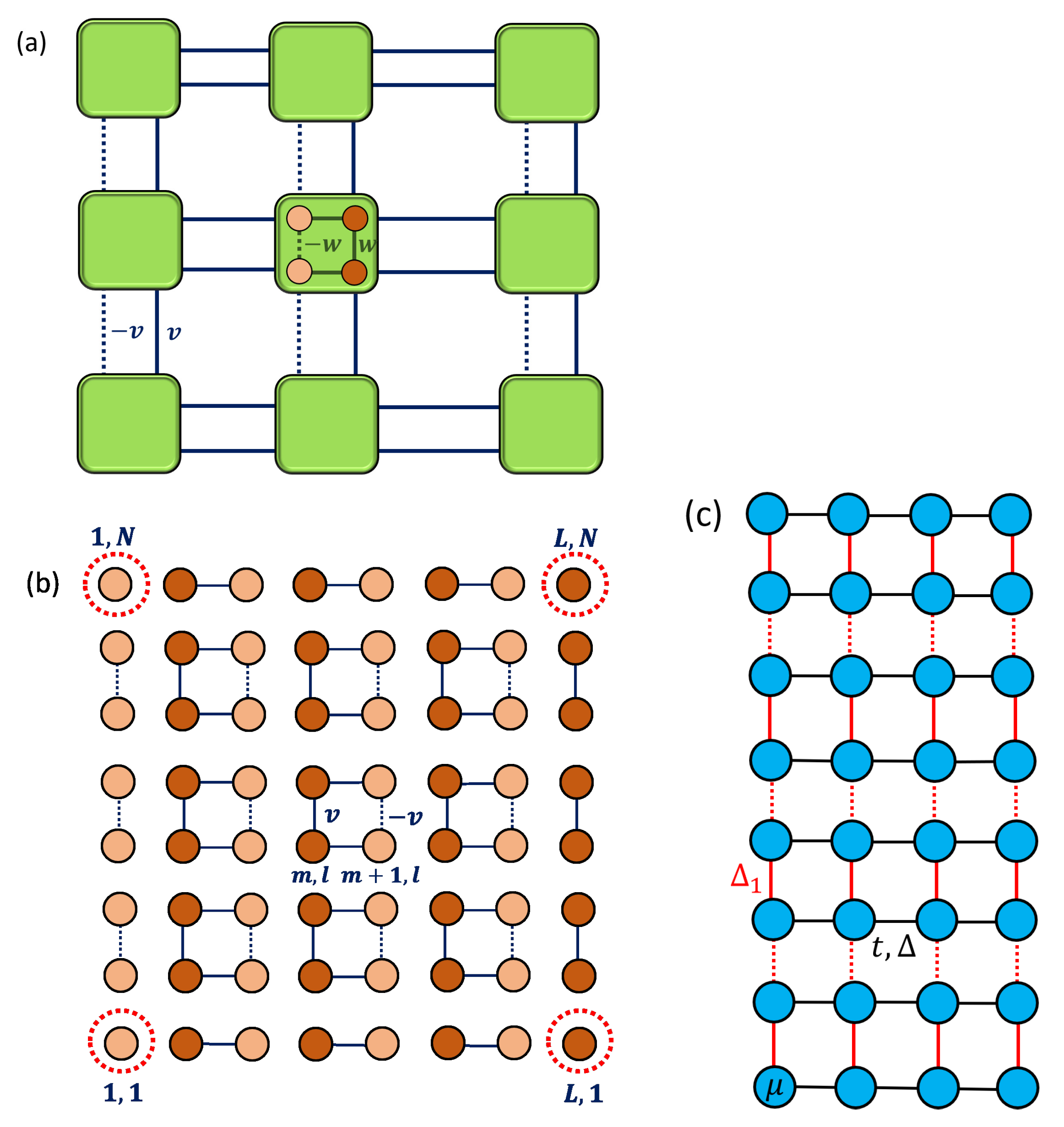
where $a_{m,l}$ and $b_{m,l}$ are the Majorana modes associated to a complex fermion operator $c_{m,l}=(a_{m,l}+i{b}_{m,l})/2$, L and N are, respectively, the length and the width of the system, m and l are the lattice sites. The lattice representation of our model is reported in Figure 1, panel (a), where the green plaquette is the unit cell and the Majorana operators a and b of Equation (1) are represented by two circles of different colors. In panel (b) of the same figure, we show the topological fully dimerized limit with $w=0$, $v\ne 0$, which generalizes the same well-known limit discussed for the SSH model in [18]. In this limit, the four Majorana modes $a_{11}$, $a_{1,N}$, $b_{L,1}$ and $b_{L,N}$ become corner zero-energy modes which decouple from the lattice. The full topological phase diagram of the model will be discussed in Section 3. Expressing the Majorana operators in terms of complex fermion operators, the Hamiltonian in Equation (1) results in N Kitaev chains of length L coupled only by pairing terms (see Figure 1, panel (c)):

$$\begin{array}{c}\hfill \begin{array}{cc}\hfill H=& \sum _{m,l=1}^{L,N}\mu c_{m,l}^{†}{c}_{m,l}+\sum _{m,l=1}^{L-1,N}(t{c}_{m,l}^{†}{c}_{m+1,l}+\Delta c_{m,l}{c}_{m+1,l}+h.c.)\hfill \\ & +\sum _{m,l=1}^{L,N-1}({\Delta }_1{c}_{m,l}{c}_{m,l+1}+h.c),\hfill \end{array}\end{array}$$

(2)

with $\mu =w$, $t=\Delta =-v/2$ and ${\Delta }_1$:

$$\begin{array}{c}\hfill {\Delta }_1=\left\{\begin{array}{c}-iw,l=odd\hfill \\ -iv,l=even.\hfill \end{array}\right.\end{array}$$

(3)

In the next section, we will discuss the analysis of the topological phase diagram of the model by evaluating the Zak phase and the energy spectrum.

3. Topological Phase

By imposing periodic boundary conditions to the model in Equation (1), we can apply the Fourier transform. The translational invariant unit cell is given by the green plaquette in Figure 1 (panel (a)) and we obtain a $4\times 4$ matrix in the momentum space, $H=\frac{1}{2}{\Psi }_{\mathbf{k}}^{†}\tilde{H}\left(\mathbf{k}\right){\Psi }_{\mathbf{k}}$:

$$\begin{array}{c}\hfill \tilde{H}\left(\mathbf{k}\right)=\left(\begin{array}{cccc}0& iw-iv{e}^{-i{k}_x}& -iw+iv{e}^{-i{k}_y}& 0\\ -iw+iv{e}^{i{k}_x}& 0& 0& iw-iv{e}^{-i{k}_y}\\ iw-iv{e}^{i{k}_y}& 0& 0& iw-iv{e}^{-i{k}_x}\\ 0& -iw+iv{e}^{i{k}_y}& -iw+iv{e}^{i{k}_x}& 0\end{array}\right),\end{array}$$

(4)

where: ${\Psi }_{\mathbf{k}}={\left(a_{m,l}\left(\mathbf{k}\right)b_{m,l}\left(\mathbf{k}\right)a_{m,l+1}\left(\mathbf{k}\right)b_{m,l+1}\left(\mathbf{k}\right)\right)}^T$ and $\mathbf{k}=(k_x,k_y)$.

The operator in Equation (4) satisfies reflection symmetries with reflection operators $m_x$, $m_y$ exchanging, respectively, $x\to -x$, $y\to -y$ and, therefore, $k_x\to -k_x$, $k_y\to -k_y$:

$$\begin{array}{c}\hfill \begin{array}{c}\hfill m_x\tilde{H}(k_x,k_y)m_x^{†}=\tilde{H}(-k_x,k_y)\\ \hfill m_y\tilde{H}(k_x,k_y)m_y^{†}=\tilde{H}(k_x,-k_y),\end{array}\end{array}$$

(5)

where $m_x={\sigma }_z\otimes {\sigma }_y$ and $m_y={\sigma }_y\otimes \mathbb{I}$. Because of the simple structure, the lattice is also invariant under rotations by $\theta =\pi /2$ up to a gauge transformation. The $C_4$ symmetry, describing the rotation, is associated to the operator $R_4$ exchanging $(k_x,k_y)\to (k_y,-k_x)$:

$$\begin{array}{c}\hfill R_4\tilde{H}(k_x,k_y)R_4^{†}=\tilde{H}(k_y,-k_x),R_4=\left(\begin{array}{cc}-{\sigma }_{+}& \frac{{\sigma }_0-{\sigma }_3}{2}\\ -\frac{{\sigma }_0+{\sigma }_3}{2}& {\sigma }_{-}\end{array}\right),\end{array}$$

(6)

where ${\sigma }_{\pm }=({\sigma }_1\pm i{\sigma }_2)/2$, ${\sigma }_0$ is the identity, ${\sigma }_i$ with $i=1\dots 3$ are the Pauli matrices and ${\left(R_4\right)}^4=-1$. The Hamiltonian in Equation (4) also satisfies particle-hole $\mathcal{P}=\mathbb{I}K$, with $\mathbb{I}={\sigma }_0\otimes {\sigma }_0$ and K the complex conjugation, time reversal $\mathcal{T}={\sigma }_z\otimes {\sigma }_{z}K$ and chiral symmetries $\mathcal{C}={\sigma }_3\otimes {\sigma }_3$:

$$\begin{array}{c}\hfill \begin{array}{cc}& \mathcal{P}\tilde{H}(k_x,k_y){\mathcal{P}}^{†}=-\tilde{H}(-k_x,k_y)\hfill \\ & \mathcal{T}\tilde{H}(k_x,k_y){\mathcal{T}}^{†}=\tilde{H}(-k_x,-k_y)\hfill \\ & \mathcal{C}\tilde{H}(k_x,k_y){\mathcal{C}}^{†}=-\tilde{H}(k_x,k_y),\hfill \end{array}\end{array}$$

(7)

thus the model belongs to the trivial two-dimensional $BDI$ class [19].

Indeed, the Berry curvature $\mathbf{B}=\nabla \wedge \mathbf{A}$ vanishes everywhere in the Brillouin zone due to the coexistence of $\mathcal{T}$ and reflection symmetries. Here, ${\mathbf{A}}_{n,m}=\langle {\psi }_n\left|i{\partial }_{\mathbf{k}}\right|{\psi }_m$ and $|{\psi }_m\rangle$ is the Bloch wave function associated with the m band. However, the reflection symmetries of Equation (5) ensure fractional quantized components of the polarization:

$$\begin{array}{c}\hfill \mathbf{P}=\frac{1}{2\pi }{\int }_{BZ}d{k}_{x}d{k}_{y}Tr\left[\mathbf{A}(k_x,k_y)\right].\end{array}$$

(8)

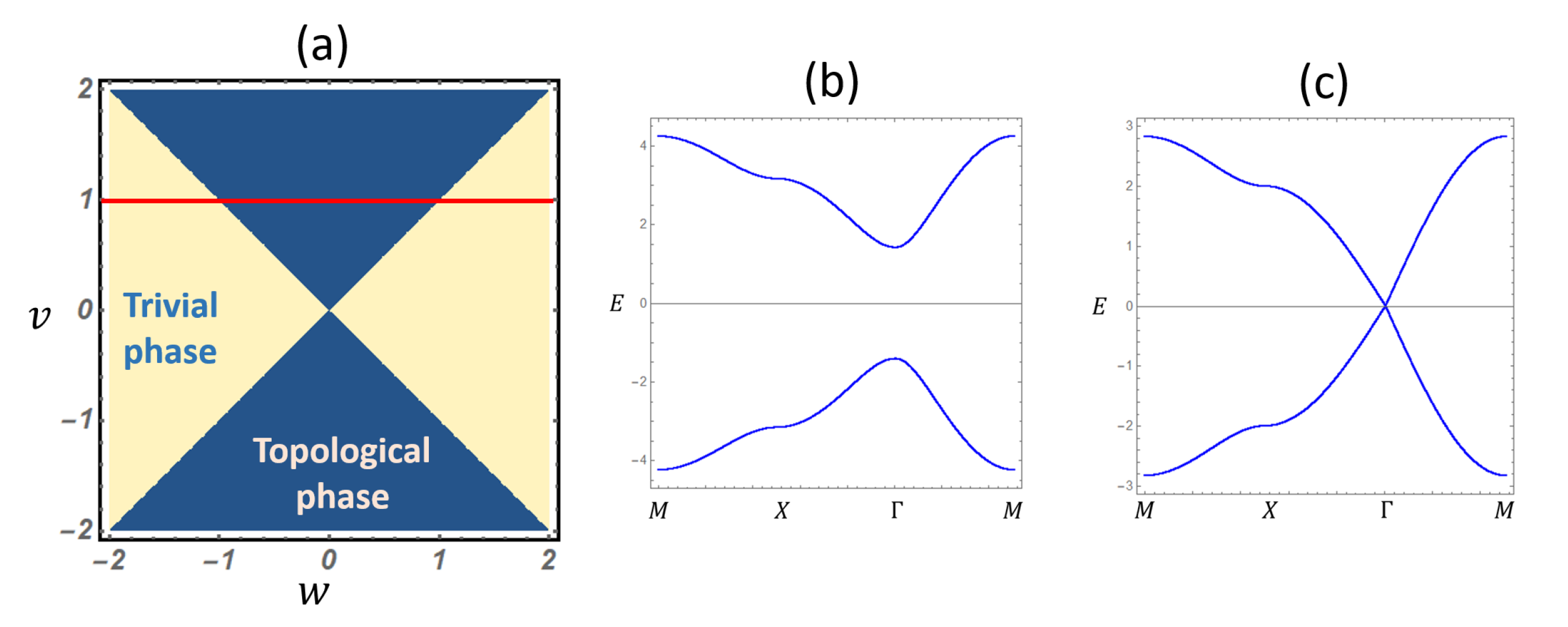
$\mathbf{P}$ is also known as a 2D Zak phase [20,21]. In particular, the 2D Zak phase takes the value $\mathbf{P}=(1/2,1/2)$ in a non-trivial phase and $\mathbf{P}=(0,0)$ in the trivial one. The presence of $C_4$ symmetry ensures that the model described is a second-order topological system with intrinsic Majorana corner states associated to the fractional quantized values of $\mathbf{P}$, which cannot be removed by a change of boundary preserving the bulk [22]. Indeed, for systems with spatial symmetries, the simultaneous presence of standard symmetries ($\mathcal{C}$, $\mathcal{P}$, $\mathcal{T}$) and crystalline symmetries is essential to realize a second-order topology. In analogy with the Aharonov–Bohm (AB) effect for a magnetic field [23], one observes the presence of a quantized charge polarization in the absence of the Berry curvature; this phenomenon gives rise to the higher order topological superconductivity [5,6,7,8,9,22]. In Figure 2 panel (a), we report the topological phase diagram (PD) of our system, which falls in a non-trivial regime for $\left|w\right|<\left|v\right|$. Panels (b) and (c) of the same figure show the band structure along the path in $\mathbf{k}$-space: $M\to X\to \Gamma \to M$, with $M=(\pi ,\pi )$, $X=(\pi ,0)$, $\Gamma =(0,0)$. The energy bands are doubly degenerate and invariant under the exchange of $w\to v$:

$$\begin{array}{c}\hfill E_{\pm }=\pm \sqrt{2}{e}^{-i(k_x+k_y)}\sqrt{e^{2i(k_x+K_y)}[v^2+w^2-vw(cos{k}_x+cos{k}_y)]}.\end{array}$$

(9)

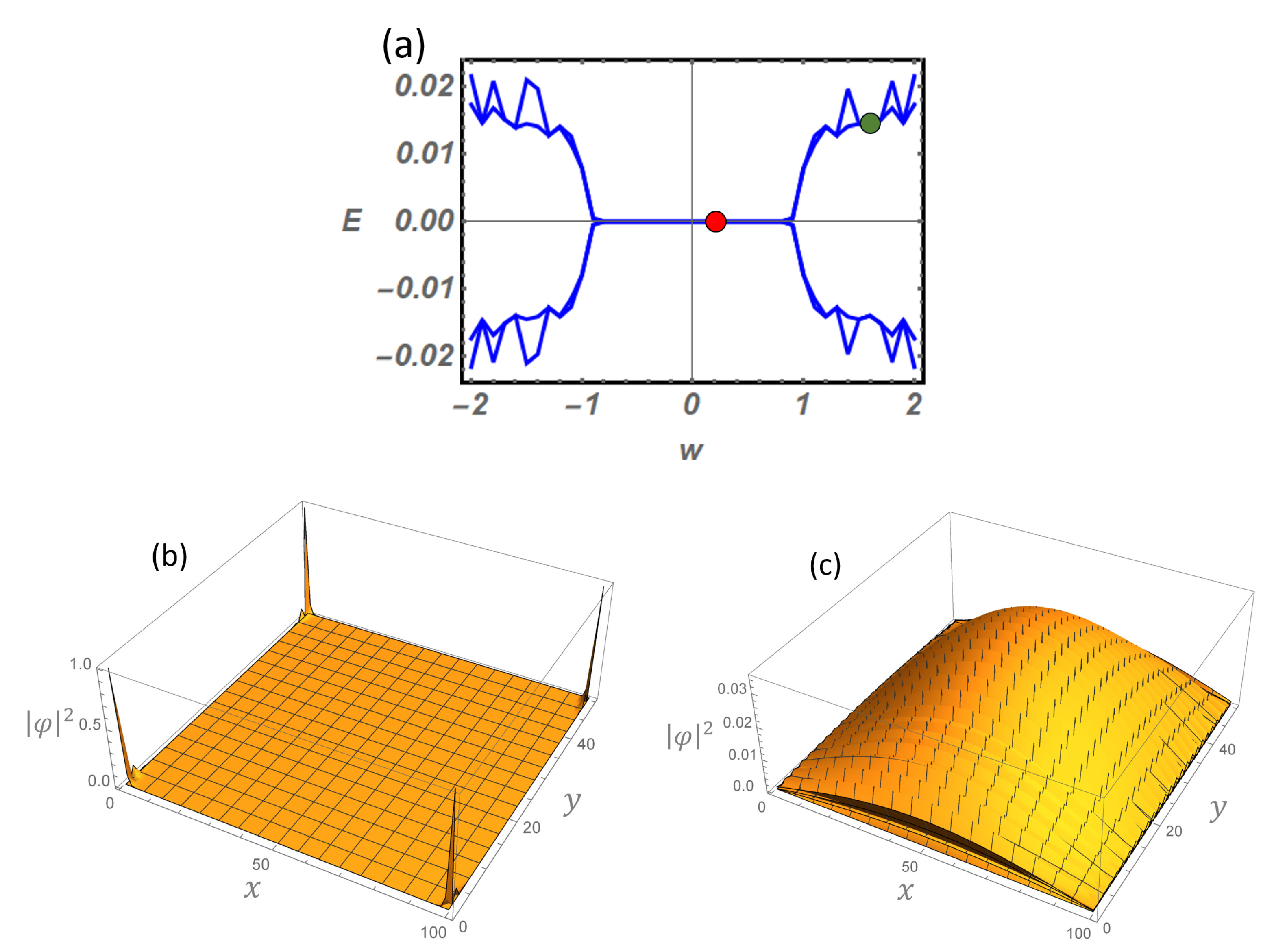
More precisely, the system shows a phase transition at the critical point $w=v$, as can be seen from the gap closing at $\Gamma =(0,0)$ point in panel (c) ($w=v=1$). Panel (b) of Figure 2 shows the bands for the points ($w=2$, $v=1$) and ($w=1$, $v=2$), in the trivial and non-trivial region, respectively. Looking at the expression of the energy bands in Equation (9), the two points are indistinguishable from the bulk properties point of view and a check of the bulk-edge correspondence is needed to show the different behaviour of topological and trivial points. To this end, in Figure 3, a system of finite size, $L=100$ and $N=50$, is analyzed. Panel (a) of Figure 3 shows the lowest energy spectrum of the system following the horizontal red cut in the phase diagram of Figure 2a. Here, we observe the expected correspondence between the gap closing and the appearance of non-trivial states. Non-trivial topological corner states associated with 2D Zak phases are shown in panel (b) of Figure 3, where we fix the parameters to those corresponding to the red circle of panel (a). In panel (c), we fix the parameters in the trivial phase corresponding to the green circle of panel (a) where the modulus square of the wavefunction does not show edge or corner states. In panels (b) and (c), x and y indicate the real space directions.

4. Topological Properties of Finite Size Systems

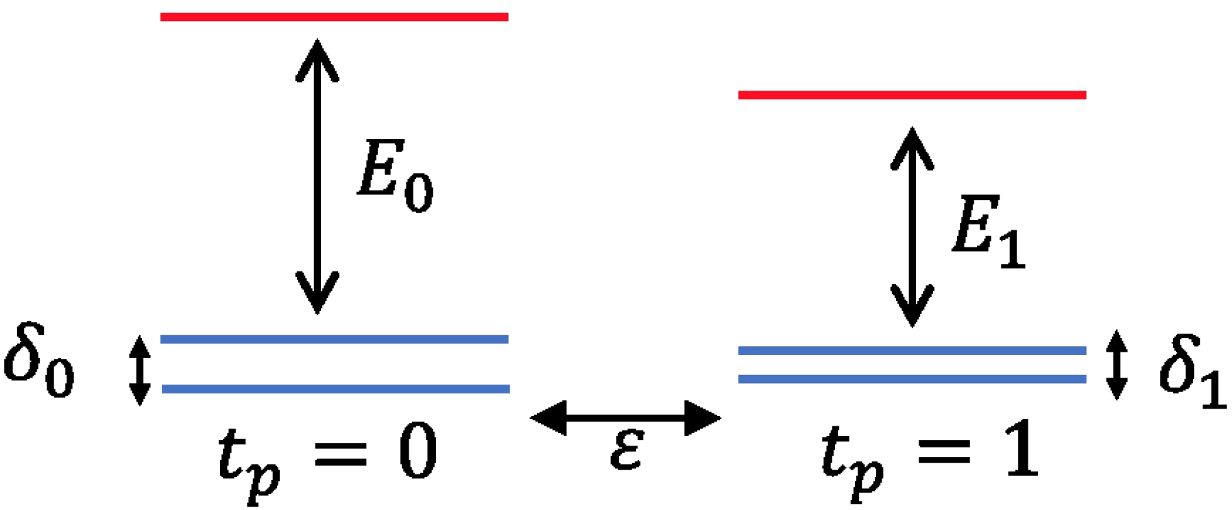
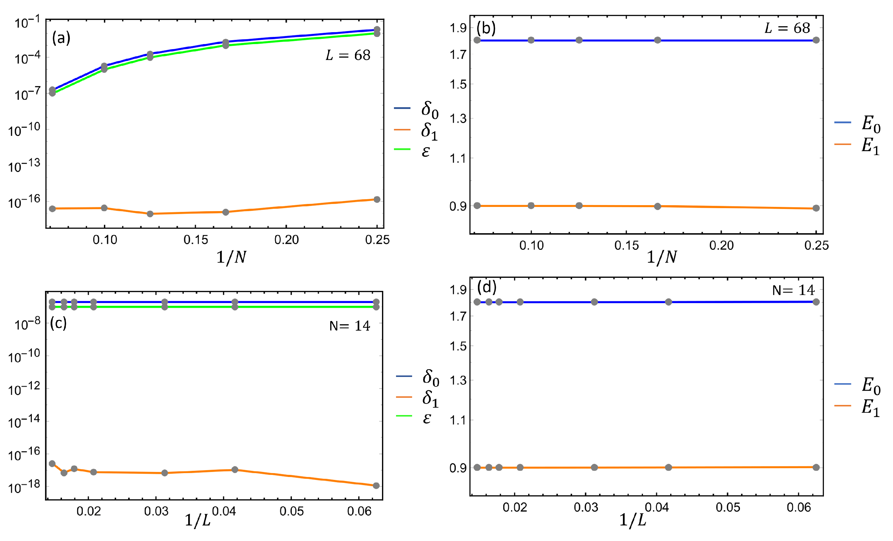
In the thermodynamic limit, when $\left|w\right|<\left|v\right|$, we have seen that the Majorana BBH model exhibits four Majorana corner modes and the ground state manifold is fourfold degenerate. In particular, since the model preserves the parity, the system is twofold degenerate for every parity sector. If the size is finite, there is a weak coupling between Majorana corner states, which decreases as the system size increases. In Figure 4, we report a scheme of the three lowest energy levels for the two parity sectors for a finite size strip and set the parameters in the topological regime. To analyze the topological properties of the finite size system, we study the behavior of: (a) the gaps between ground states and first excited states indicated by ${\delta }_0$, and ${\delta }_1$, (b) the energy separation between the second and third excited states, indicated by $E_0$ and $E_1$ and (c) the energy separation between the ground states corresponding to the two different parities ($ϵ$). The subscripts 0, 1 represent the two parities. In the thermodynamic limit, fixing the parameters in a topological point of the phase diagram, the following asymptotic limits are expected: ${\delta }_0\to 0$, ${\delta }_1\to 0$, $ϵ\to 0$, while $E_0$ and $E_1$ should remain finite. More precisely, the manifold gaps ${\delta }_0$, ${\delta }_1$ and $ϵ$ are expected to decay exponentially to zero, while increasing the system size. Actually performing the analysis of the manifold gaps and of $ϵ$ while varying the size of the system is the best way to test the robustness of non-trivial regime.

In Figure 5, we show the finite size scaling of ${\delta }_i$, $ϵ$ (panels (a) and (c)) and $E_i$ (panels (b) and (d)) with $i=0,1$, setting the parameters in a non-trivial point of the phase diagram ($w=0.1$, $v=1$). More precisely, in panels (a) and (b), we fix the length $L=68$ and consider different values of the width of the strip $N=4$, 6, 8, 10, 14, while in panels (c) and (d), we fix the width $N=14$ and consider the lengths $L=16$, 24, 32, 48, 56, 61, 68. In both (c) and (d), the gap energies $E_0$, $E_1$ remain finite at increasing sizes, as expected in a topological phase, on the other ${\delta }_0$ and ${\delta }_1$ decay exponentially to zero at increasing widths N (panel (a)), while for a fixed $N=14$ they are already very small and remain almost constant with increasing lengths L (panel (c)). $ϵ$, on the other hand, turns out to be comparable, for all the considered sizes, to the machine error. This behavior of the gaps ensures that the topological phase of the system is robust.

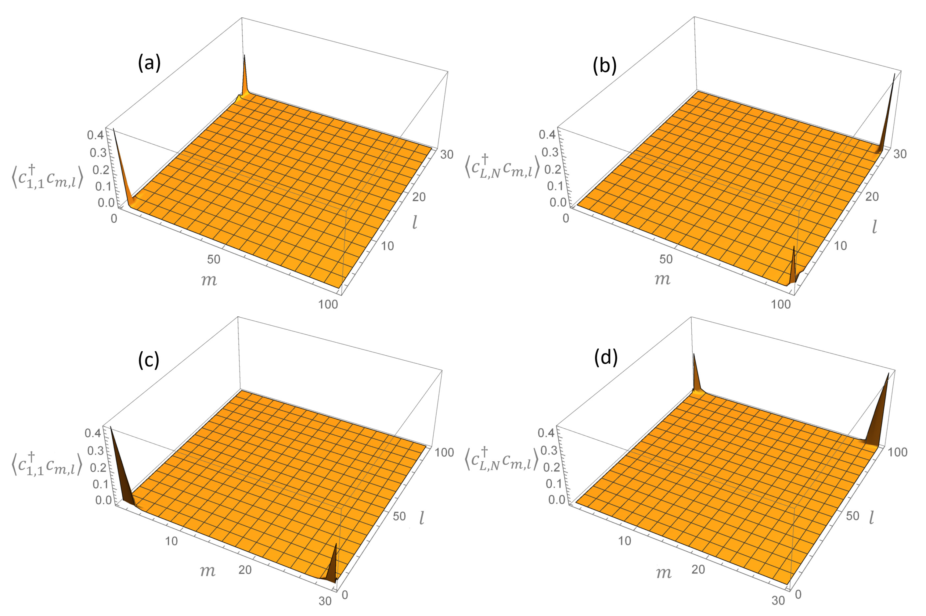
To gain further insight into the topological properties of the finite size system in Figure 6, we show the non-local fermion correlations, where panels (a) and (b) correspond to $<c_{1,1}^{†}{c}_{m,l}>$ and $<c_{L,N}^{†}{c}_{m,l}>$, respectively, with lattice indices l and m running along the length and the rung of the strip with $L=100$ and $N=30$. The shorthand notation $<c_{1,1}^{†}{c}_{m,l}>$ and $<c_{L,N}^{†}{c}_{m,l}>$ instead of $\langle GS{c}_{1,1}^{†}{c}_{m,l}GS\rangle$ and $\langle GS{c}_{L,N}^{†}{c}_{m,l}GS\rangle$ is used, with $|GS\rangle$ being the many body ground state. All the details about the formulas used to compute the fermion correlations are reported in Appendix A. As we can see, the fermionic states are always correlated along the shortest directions $(1,1)-(1,N)$ and $(L,1)-(L,N)$. The same behavior is observed when the dimensions of the strip are exchanged $L\to N$, $N\to L$. In panels (c) and (d) of Figure 6, we report the non-local fermion correlations of a Majorana BBH strip with $L=30$ and $N=100$. We observe the tendency of the system to form topological modes that correlate along the shortest dimension. A finite size square system $L=N$ is thus the best configuration to observe the formation of Majorana fermions at the corners.

5. Conclusions

We have proposed and analyzed the topological phases of a Majorana BBH model, consisting of a Majorana $2D$ SSH model with a synthetic magnetic flux of $\pi$. Due to the coexistence of ${\mathrm{C}}_4$ symmetry and reflection symmetries, the system turns out to be a second-order topological superconductor with a quantized 2D Zak phase in the absence of Berry curvature. Starting from the Hamiltonian in k-space, we have studied the topological phases of the system, showing the bulk-edge correspondence and the formation of Majorana corner states. To study the robustness of the topological phase, we have analyzed the finite size scaling of the gaps between the ground states and the first excited states in the two parity sectors and found the expected exponential decay with the system length. The analysis of the fermion non-local correlation functions shows that the Majorana zero modes nucleate at the corners of the system, correlating along the shortest dimension.

Our model could be realized in photonics systems or in cold atoms platforms where a high efficiency to control parameters through gauge fields has been demonstrated. We believe that our proposal opens new directions in inducing unique corner states by gauge field and offering possibilities to design $2D$ models with non-zero Zak phase and robust edge states. Various directions remain open, among which the study of the effect of interactions on the higher order topological phase is a relevant one.

References

- Schindler, F.; Cook, A.M.; Vergniory, M.G.; Wang, Z.; Parkin, S.S.P.; Bernevig, B.A.; Neupert, T. Higher-order topological insulators. Sci. Adv. 2018, 4. [Google Scholar] [CrossRef] [PubMed] [Green Version]
- Benalcazar, W.A.; Bernevig, B.A.; Hughes, T.L. Quantized electric multipole insulators. Science 2017, 357, 61–66. [Google Scholar] [CrossRef] [PubMed] [Green Version]
- Langbehn, J.; Peng, Y.; Trifunovic, L.; von Oppen, F.; Brouwer, P.W. Reflection-Symmetric Second-Order Topological Insulators and Superconductors. Phys. Rev. Lett. 2017, 119, 246401. [Google Scholar] [CrossRef] [PubMed] [Green Version]
- Benalcazar, W.A.; Bernevig, B.A.; Hughes, T.L. Electric multipole moments, topological multipole moment pumping, and chiral hinge states in crystalline insulators. Phys. Rev. B 2017, 96, 245115. [Google Scholar] [CrossRef] [Green Version]
- Teo, J.C.Y.; Hughes, T.L. Existence of Majorana-Fermion Bound States on Disclinations and the Classification of Topological Crystalline Superconductors in Two Dimensions. Phys. Rev. Lett. 2013, 111, 047006. [Google Scholar] [CrossRef]
- Yan, Z.; Bi, R.; Wang, Z. Majorana Zero Modes Protected by a Hopf Invariant in Topologically Trivial Superconductors. Phys. Rev. Lett. 2017, 118, 147003. [Google Scholar] [CrossRef] [PubMed] [Green Version]
- Khalaf, E. Higher-order topological insulators and superconductors protected by inversion symmetry. Phys. Rev. B 2018, 97, 205136. [Google Scholar] [CrossRef] [Green Version]
- Hsu, C.H.; Stano, P.; Klinovaja, J.; Loss, D. Majorana Kramers Pairs in Higher-Order Topological Insulators. Phys. Rev. Lett. 2018, 121, 196801. [Google Scholar] [CrossRef] [Green Version]
- You, Y.; Litinski, D.; von Oppen, F. Higher-order topological superconductors as generators of quantum codes. Phys. Rev. B 2019, 100, 054513. [Google Scholar] [CrossRef] [Green Version]
- Mittal, S.; Orre, V.; Zhu, G. Photonic quadrupole topological phases. Nat. Photonics 2019, 13, 692–696. [Google Scholar] [CrossRef] [Green Version]
- Xu, X.W.; Li, Y.Z.; Liu, Z.F.; Chen, A.X. General bounded corner states in the two-dimensional Su-Schrieffer-Heeger model with intracellular next-nearest-neighbor hopping. Phys. Rev. A 2020, 101, 063839. [Google Scholar] [CrossRef]
- Serra-Garcia, M.; Peri, V.; Süsstrunk, R. Observation of a phononic quadrupole topological insulator. Nature 2018, 555, 342–345. [Google Scholar] [CrossRef] [PubMed]
- Serra-Garcia, M.; Süsstrunk, R.; Huber, S.D. Observation of quadrupole transitions and edge mode topology in an LC circuit network. Phys. Rev. B 2019, 99, 020304. [Google Scholar] [CrossRef] [Green Version]
- Peterson, C.W.; Benalcazar, W.A.; Hughes, T.L.; Bahl, G. A quantized microwave quadrupole insulator with topologically protected corner states. Nature 2018, 555, 346–350. [Google Scholar] [CrossRef]
- Harari, G.; Bandres, M.A.; Lumer, Y.; Rechtsman, M.C.; Chong, Y.D.; Khajavikhan, M.; Christodoulides, D.N.; Segev, M. Topological insulator laser: Theory. Science 2018, 359. [Google Scholar] [CrossRef] [PubMed] [Green Version]
- Kim, H.; Wang, M.; Smirnova, D. Multipolar lasing modes from topological corner states. Nat. Commun. 2020, 11. [Google Scholar] [CrossRef]
- Pahomi, T.E.; Sigrist, M.; Soluyanov, A.A. Braiding Majorana corner modes in a second-order topological superconductor. Phys. Rev. Res. 2020, 2, 032068. [Google Scholar] [CrossRef]
- Su, W.P.; Schrieffer, J.R.; Heeger, A.J. Solitons in Polyacetylene. Phys. Rev. Lett. 1979, 42, 1698–1701. [Google Scholar] [CrossRef]
- Altland, A.; Zirnbauer, M.R. Nonstandard symmetry classes in mesoscopic normal-superconducting hybrid structures. Phys. Rev. B 1997, 55, 1142–1161. [Google Scholar] [CrossRef] [Green Version]
- Resta, R. Macroscopic polarization in crystalline dielectrics: The geometric phase approach. Rev. Mod. Phys. 1994, 66, 899–915. [Google Scholar] [CrossRef]
- Liu, F.; Wakabayashi, K. Novel Topological Phase with a Zero Berry Curvature. Phys. Rev. Lett. 2017, 118, 076803. [Google Scholar] [CrossRef] [PubMed] [Green Version]
- Trifunovic, L.; Brouwer, P.W. Higher-Order Topological Band Structures. Phys. Status Solidi 2021, 258, 2000090. [Google Scholar] [CrossRef]
- Thouless, D.J. Topological Quantum Numbers in Nonrelativistic Physics; World Scientific: Singapore, 1998. [Google Scholar]
- Eisler, V.; Zimborás, Z. On the partial transpose of fermionic Gaussian states. New J. Phys. 2015, 17, 053048. [Google Scholar] [CrossRef]
- Tsvelik, A.M. Quantum Field Theory in Condensed Matter Physics, 2nd ed.; Cambridge University Press: Cambridge, UK, 2003. [Google Scholar] [CrossRef]
- Molinari, L.G. Notes on Wick’s theorem in many-body theory. arXiv 2017, arXiv:math-ph/1710.09248. [Google Scholar]
Figure 1.
(a) Lattice geometry in the Majorana basis, the green plaquette identifies the translational invariant unit cell, while pink and brown circles are the Majorana modes a and b associated with a complex fermionic mode. w and v are, respectively, the intracell and intercell couplings, a dashed line indicates a negative coupling. (b) Fully dimerized limit of the lattice model depicted in panel (a) with and . The mapping to complex fermionic modes is shown in panel (c) for generic w, v. Indeed, in (c), the following identities hold: , and is staggered, with associated with continuous red lines and associated to dashed red lines.
Figure 2.
(a) Topological phase diagram of a 2D Majorana Benalcazar–Bernevig–Hughes (BBH) model in the parameter space v, w. Blue and yellow regions identify the topological and trivial phases, respectively. The red horizontal line is the cut at which we evaluate the lowest energy spectrum in Figure 3 panel (a). Panel (b) shows the spectrum along the path in the Brillouin zone in a trivial (topological) phase , (, ) and panel (c) shows the spectrum at the phase transition point .
Figure 3.
(a) Low energy spectrum of a strip following the horizontal red cut of Figure 2 panel (a). Here, w is in units of v. In panel (b), we show the square modulus of the lowest four energy modes corresponding to a gap closing point (red point of panel (a)) and in the gapped phase (green point of panel (a)). The sizes of the strip for all the plots are and .
Figure 4.
Scheme of the lowest energy many body states in a strip with finite size and in a topological point of the phase diagram. denotes the even, odd parity sector, and are the energy gaps between the ground states and the first excited states, and are the energy separation between the second and the first excited states, is the energy separation between the ground states of the two parity sectors and the subscripts 0 and 1 denote the parities.
Figure 5.
Plots of the energy gaps at varying the sizes of the Majorana BBH strip L and N, as in the panel labels. In panel (a,b), the length is fixed and the behavior of , , (panel (a)) and , (panel (b)) are plotted for different values of the width , 6, 8, 10, 14. The same plots obtained by fixing and considering , 24, 32, 48, 56, 61, 68 are reported in panels (c,d). The model parameters have been fixed as , .
Figure 6.
Fermion correlations (panels (a,c)) and (panels (b,d)) for a strip with , (panels (a,b)) and , (panels (c,d)). The lattice sites indices are m and l, and the parameters have been fixed in a topological point: , .
Publisher’s Note: MDPI stays neutral with regard to jurisdictional claims in published maps and institutional affiliations. |
© 2021 by the authors. Licensee MDPI, Basel, Switzerland. This article is an open access article distributed under the terms and conditions of the Creative Commons Attribution (CC BY) license (https://creativecommons.org/licenses/by/4.0/).
Share and Cite
MDPI and ACS Style
Maiellaro, A.; Citro, R. Topological Edge States of a Majorana BBH Model. Condens. Matter 2021, 6, 15. https://0-doi-org.brum.beds.ac.uk/10.3390/condmat6020015
AMA Style
Maiellaro A, Citro R. Topological Edge States of a Majorana BBH Model. Condensed Matter. 2021; 6(2):15. https://0-doi-org.brum.beds.ac.uk/10.3390/condmat6020015
Chicago/Turabian StyleMaiellaro, Alfonso, and Roberta Citro. 2021. "Topological Edge States of a Majorana BBH Model" Condensed Matter 6, no. 2: 15. https://0-doi-org.brum.beds.ac.uk/10.3390/condmat6020015