
Critical Temperature in the BCS-BEC Crossover with Spin-Orbit Coupling


1
Dipartimento di Fisica e Astronomia “G. Galilei”, University of Padova, Via F. Marzolo 8, 35151 Padova, Italy
2
Padua Quantum Technologies Research Center, University of Padova, Via Gradenigo 6/b, 35131 Padova, Italy
3
ICFO-Institut de Ciencies Fotoniques, The Barcelona Institute of Science and Technology, Castelldefels, 08860 Barcelona, Spain
*
Author to whom correspondence should be addressed.
Condens. Matter 2021, 6(2), 16; https://0-doi-org.brum.beds.ac.uk/10.3390/condmat6020016
Submission received: 31 March 2021
/
Revised: 26 April 2021
/
Accepted: 27 April 2021
/
Published: 30 April 2021
(This article belongs to the Special Issue Fluctuations and Highly Non-linear Phenomena in Superfluids and Superconductors III)
Abstract
:We review the study of the superfluid phase transition in a system of fermions whose interaction can be tuned continuously along the crossover from Bardeen–Cooper–Schrieffer (BCS) superconducting phase to a Bose–Einstein condensate (BEC), also in the presence of a spin–orbit coupling. Below a critical temperature the system is characterized by an order parameter. Generally a mean field approximation cannot reproduce the correct behavior of the critical temperature over the whole crossover. We analyze the crucial role of quantum fluctuations beyond the mean-field approach useful to find along the crossover in the presence of a spin–orbit coupling, within a path integral approach. A formal and detailed derivation for the set of equations useful to derive is performed in the presence of Rashba, Dresselhaus and Zeeman couplings. In particular in the case of only Rashba coupling, for which the spin–orbit effects are more relevant, the two-body bound state exists for any value of the interaction, namely in the full crossover. As a result the effective masses of the emerging bosonic excitations are finite also in the BCS regime.
1. Introduction
Experimental developments in confining, cooling and controlling the strength of the interaction of alkali atoms brought a lot of attention to the physics of the crossover between two fundamental and paradigmatic many-body systems, the Bose–Einstein condensation (BEC) and the Bardeen–Cooper–Schrieffer (BCS) superconductivity.
A system of weakly attracting fermions can be treated in the context of the well-known BCS theory [1], originally formulated to describe superconductivity in some materials where an effective attractive interaction between electrons can arise from electron-phonon interaction. This theory predicts a phase transition and the formation of the so-called Cooper pairs [2] with the appearance of a gap in the single particle spectrum. The fermions composing these weakly bounded pairs are spatially separated since their correlation length is larger than the mean inter-particle distance; for this reason the pairs cannot be considered as bosons. By increasing the strength of the attraction among the fermions, the system could be seen as made of more localized Cooper pairs, or almost bosonic molecules, which may undergo into a true Bose–Einstein condensation. Since there is no evidence of a broken symmetry by continuously varying the width of the couples, this process realizes a crossover between a BCS and a BEC state. The idea of this crossover preceded by far its experimental realization [3] and became a subject of active investigations by several authors. Those studies were first motivated by the purpose of understanding superconductivity in metals at very low electron densities, since in this diluted regime Cooper pairs are smaller than the mean inter-particle distance and, therefore, can be treated like bosons. In a particularly relevant pioneering work [4] a system of interacting fermions has been investigated to obtain the evolution of the critical temperature of the system along the crossover by changing the strength of the interaction between the BCS and the BEC limits. [5] The discovery of the high-temperature superconductors [6], where the coupling between electrons is supposed to be stronger than that in conventional superconductors, renewed the interest in the BCS-BEC crossover with the aim to explore the regime of stronger interaction. Few years later, an important work [7] provided for the first time a path integral formulation of the problem, which we will review here, describing the crossover at finite temperature with tunable strength of the coupling between pairs. The scientific interest in this field was first purely theoretical because the interaction strength in real solid state materials cannot be tuned easily. The situation changed drastically after the first realizations of magnetically confined ultracold alkali gases. A typical alkali gas obtained in laboratory is made by to atoms, with a density n inside the bulk of a realistic trap in the range from to cm. An important property is their diluteness: these densities are such that the mean inter-particle distance is larger than the length scale associated to the atom-atom potential and implying that only two-body physics is relevant. Below those densities, the thermalization of the gas after a perturbation becomes too slow, while at higher densities three body collisions become relevant. At low temperatures, namely at low kinetic energies, the scattering properties of the atoms can be characterized by a single parameter, the scattering length. These gases can be furthermore cooled at such temperatures to enter in a quantum degenerate regime characterized by a thermal de Broglie wavelength of the same order of the interatomic distance, i.e., . The degenerate temperatures, for the densities mentioned before, are smaller than a . These are the conditions achieved in the first experimental realization of a Bose–Einstein condensation [8]. The importance of such experimental setups does not rely only on these extreme conditions, but also on the possibility of fine tuning the parameters which describe the gas. In particular the mechanism of the so-called Feshbach resonance allows one to control the strength of the interaction between two atoms by simply a magnetic field, for example, making it sufficiently strong to support a new bound state. This phenomenon was first predicted and then observed experimentally [9,10] in bosonic systems. Soon after these techniques have been extended to create and manipulate ultracold gases for fermionic systems [11,12,13,14] employing atomic alkali gases with two different components, a mixture of atoms in two different spin or pseudospin states, where the quantum degeneracy is reached when lowering the temperature the energy of the system ceases to depend on the temperature. In this system by Feshbach resonance the interaction among the atoms can be made sufficiently strong to allow the formation of a two-body bound state, called Feshbach molecule, with a lifetime compatible to the time needed to cool the system down and to observe a Bose–Einstein condensation. Later the experimental observation of fermionic pairs was extended to the whole region of the crossover [15,16], studying also the thermodynamical properties [17,18]. A renewed interest in the study of the BCS-BEC crossover arose in 2011 after the experimental realization, in the context of ultracold gases, of a synthetic spin–orbit (SO) interaction [19,20,21,22]. In contrast to the spin–orbit interaction in solid state systems, in atomic gases this coupling is produced by means of laser beams and therefore is perfectly tunable. The realization of this artificial spin–orbit coupling is a bright example of the versatility and controllability of the ultracold techniques, showing once more that ultracold gases are the perfect experimental playgrounds for testing physical models hardly realizable by means of other solid state setups. These experimental achievements stimulated intense theoretical effort to understand the spin–orbit effects with the so-called Rashba [23] and Dresselhaus [24] terms in the evolution from BCS to BEC superfluidity, considering many SO configurations, in two and three dimensions, at zero and finite temperature, exploring eventually novel phases of matter or topological properties [25,26,27,28,29,30,31,32,33,34,35,36,37,38,39,40,41,42,43,44,45,46,47,48,49,50,51,52,53,54,55,56,57,58,59,60,61,62,63,64,65,66,67]. In particular SO coupling induces triplet pairing [43] which can produce nodes in the quasiparticle excitation spectrum. This allows for detecting bulk topological phase transitions of the Lifshitz type in polarized systems [41] or, more recently, in heterostructures [68]. Moreover the experimental realization of 2D degenerate Fermi gases for ultracold atoms in a highly anisotropic disk-shaped potential [69] is one of the reasons of the growing interest for fermions in reduced dimensionality, where exotic gapless superfluid states and Fulde–Ferrell–Larkin–Ovchinnikov (FFLO) pairing states can be observed [55].
The aim of this paper is to review some basic concepts on the BCS-BEC crossover, whose properties will require taking into account quantum fluctuations in order to get a better theoretical predictions when comparing with experimental results [70]. We will reproduce many results beyond the mean-field level, and extend the study in the presence of a spin–orbit interaction, in a detailed and comprensive way, by means of a path integral approach, with a particular emphasis to the derivation of the critical temperature . We will show how can be strongly enhanced by the SO couplings in the BCS side, already at the mean-field level, while its increase is softened by the effects of the quantum fluctuations specially in the intermediate region of the crossover and in the strong coupling regime.
1.1. Basic Concepts in Ultracold Atomic Physics
To understand the structure of an atom it is necessary to consider the forces among its constituents. For alkali atoms (Li, Na, K, Rb...), the relevant force is due to Coulomb interaction that acts between the off-shell electron and the effective charge of the nucleus. This central force produces the following Bohr energy spectrum
with , where is the so-called fine structure constant and the reduced mass, approximately given by the mass of the electron. This spectrum is degenerate in the quantum numbers L and , associated to the angular momentum operators and .
The Coulomb interaction, due to its symmetry, preserves the angular momentum and the spin separately. However, in principle, they are coupled via a spin–orbit term, , therefore, only the total angular momentum is conserved. This additional term causes the known correction to the spectrum, called fine structure, shifting the degeneracy in the energy spectrum by . However, for ultracold alkali gases, at very low temperatures, only the fundamental state is occupied, so that the off-shell electron is in the s orbital (). In this state and the spin–orbit fine structure can be neglected, . However, also the coupling between the spins of the electrons and of the nucleus can remove the degeneracies and it is generally approximated by a dipole–dipole interaction
This term, again, does not lead to the conservation of both and separately but only of the total spin of the atom , since . Then it is possible to label the states of an alkali atom by the quantum numbers F and , related to the operators and . The effect of this contribution is a small correction to the Bohr spectrum, usually called hyperfine structure
Since and because of the properties of the sums of angular momentums, the quantum number F is allowed only to have the values , so the hyperfine correction is given by
In the presence of an homogeneous magnetic field, this coupling between the latter and the electronic and nuclear spins gives rise to a shift of the energy levels of the atoms, called the Zeeman effect. An alkali atom at very low energy and in a magnetic field can be described, therefore, by the following Hamiltonian
where the Zeeman couplings are inversely proportional to the mass of the particles, therefore , since the nucleus is heavier than the electrons. As long as the effect of the magnetic field is small, F and can be considered almost good quantum numbers, while in general the eigenstates are labeled by e , associated to and . Diagonalizing the Hamiltonian in Equation (5) we can find the corrections to the Bohr spectrum. For example, in the case of an hydrogen atom and we get
The dependence on the magnetic field is quadratic for low intensities and linear for high field. An important experimental feature is that varying the magnetic field it is possible to vary the energy levels of the single atom, a property that can be exploited to induce a confining potential for atoms, realizing an atomic trap.
There are two main kinds of atomic traps available, the magnetic and the optical dipole traps, which are briefly discussed below.
- Magnetic Traps
This technique is based on the concrete possibility of creating position dependent magnetic fields which, as a consequence, make every hyperfine energies also position dependent. In these conditions an alkali atom has a kinetic energy plus an effective potential, that, properly taylored, can be seen as a confining potential for the gas,
with a confining force . Trapping a gas in a magnetic field is the key to achieve degeneracy temperatures; in these conditions the gas is isolated from the external world getting rid of the main source of heating which is due to the walls of the container. Typically the magnetic trap is modeled to obtain an harmonic potential, however there are several experimental possibilities depending only on the ability to create non homogeneous magnetic fields. In particular these potentials highly depend on the hyperfine states of the atom and this characteristic can be exploited to select particular states in the trap. Another interesting possibility is to create highly anisotropic potentials by strong confinement in some dimensions, realizing one- or two-dimensional systems. This technique is compatible with the cooling methods of atomic gases but not with the mechanism of the magnetic Feshbach resonance. For the latter reason an alternative trapping method is required.
- Optical Traps
The optical traps are based upon the interaction between an atom and light of a laser beams. The key features of this method are the great stability of the trapped gas and the possibility of making a lot of different geometries. Under proper conditions, called far-detuning, the confinement is independent from the internal state of the atom. When an atom is put in a laser beam, the electric field induces an electric dipole moment , where is the polarizability. The effective potential given by the iteration between the dipole moment and the electric field is given by a temporal mean value
which is simply directly proportional to the intensity of the beam. It is then possible to produce an artificial potential, as before, considering a position dependent focalization of the laser so that there is a force acting on the single atom given by . As mentioned, this technique makes possible to easily create different geometries. Indeed, employing two counter-propagating laser in more dimensions for example, lattice potentials can be realized, particularly interesting since they can simulate solid state systems in a fully controllable environment. For a more complete review on this confining technique one can refer to Refs. [71,72].
The confined gas has to be cooled down in order to reach the degeneracy temperatures. This can be done in two steps, by laser cooling and evaporative cooling [73].
- Laser or Doppler Cooling
The term laser cooling refers to several techniques employed to cool atomic gases, taking advantage of the interaction between light and matter. The most relevant one takes advantage also from the Doppler effect. This technique is applied to slow down the mean velocity of the atoms realizing a situation in which an atom absorbs more radiation in a direction and less in the opposite one. This can be done slightly detuning the frequency of the laser below the resonance of the exited state of the atom. Because of the Doppler effect, the atom will see a frequency closer to the resonant one and so it will have an higher absorption probability. In the opposite direction the effect will be reversed. The atom, which is now in an exited state, can spontaneously emit a photon. The overall result of the absorption and emission process is to reduce the momentum of the atom, therefore its speed. If the absorption and emission are repeated many times, the average speed, and therefore the kinetic energy of the atoms, will be reduced, and so the temperature. By this technique one can reach low temperatures of the order of some , still not enough to get a degenerate gas.
- Evaporative Cooling
The degenerate temperatures can be reached by the so-called forced evaporative cooling method. A fundamental feature of every trap discussed before is the possibility of varying its depth, defined as the energy difference between the bottom and the scattering threshold of the potential. Lowering the depth of the trap it is possible to let the most energetic atoms escape; this correspond to extracting energy from the gas at the cost of loosing a considerable quantity of matter. After the thermalization of the gas, the temperature is lowered and this procedure can be repeated. The lower limit in temperature now is related to the rate between inelastic collisions, that fix the lifetime of the sample, and the elastic collisions, that assure thermalization and fix the time needed for the cooling process. Loading more atoms in a trap lowers the limit of the lowest temperature achievable but also makes the gas unstable. With the correct compromise this scheme allows to go well below the degenerate temperatures. For alkali atoms the limits in temperatures achievable by evaporative cooling are at the order of T∼pK [74]. Once a degenerate gas is obtained, letting the gas expand in free flight by turning off the trap, from the absorption spectrum one can access to the temperature of the gas or to the density profile in position space that can be compared with theoretical results.
1.2. Artificial Spin-Orbit Interaction in Ultracold Gases
Laser techniques can be employed also to build a tunable synthetic spin–orbit coupling between two pseudo-spin states of an atom. In a previous section it was shown that spin–orbit coupling (fine structure) for atoms in the fundamental state (, ) vanishes. In order to induce it in laboratory it is necessary to select a gas with two components. In the first realization of this system [19] two states () of Rb were chosen with pseudo-spins and . In order to understand schematically how it works, let us suppose that the atom is in an initial state , then, two lasers can be tuned in such a way that one induces a transition to an intermediate exited state and the other induces a stimulated emission from the latter state to . The inverse process is equally allowed. Due to the Doppler effect, this coupling will be necessarily momentum-sensitive and, as shown in Refs. [19,20], the effective generated term is equivalent to a spin–orbit coupling of a spinful particle moving in a static electric field , let us say, along the z axis. An effective additional term in the Hamiltonian is , where is the magnetic field seen by the moving particle and the electron magnetic moment, which can be written as
This is called Rashba coupling, in analogy to the same coupling occurring in crystals. With the same technique other interactions can be produced in the laboratory such as the Dresselhaus term
or a Weyl term . The two lasers are detuned by a frequency from the Raman resonance and couple the states and with the Raman strength . This generates additional terms, and . We will neglect the detunig term and will consider the Raman coupling as an effective artificial Zeeman term
By this procedure one can study the effects of a spin–orbit interaction in ultracold gases, which has the great advantage of being fully under control, allowing for fine tuning experiments where the couplings can be easily manipulated, not possible otherwise in solid state systems.
2. Two-Body Scattering Problem
In the previous section we said that only two-body physics is relevant in a dilute ultracold gas, for that reason we will briefly review the two body problem in a generic central potential. We are going to consider only scattering properties after two-body collisions neglecting the three-body ones because of the low probability of finding three particles within the range of interaction. Generally interatomic potentials are not known analytically and their approximations are not so easy to use in theoretical and numerical evaluations. The density of the gas can fix the interparticle distances and the range of the potential. This is what typically happens in the experiments with ultracold dilute gases. In this situation an approximate potential, or pseudo-potential, can be employed, which should exhibit some general properties of the full scattering problem. A detailed analysis of the scattering problems, specifically for ultracold gases, can be found in Refs. [75,76,77]. Scattering theory provides the tools useful to characterize the interaction between particles in terms of few parameters that can be used to create suitable approximate potentials. The Schrödinger equation is employed to determine the wavefunctions and the scattering amplitudes, then we require that a simple pseudo-potential should reproduce the same results in a low energy limit, namely in the ultracold limit. We will assume that the two-body interaction is described by a short-range and spherically symmetric potential.
It is known that Schrödinger equation for the wavefunction of two colliding particles can be decomposed in one equation that describes the center-of-mass motion, a free particle equation with mass , and another that describes the relative motion. With the definition for the reduced mass, in the relative frame the Schödinger equation reads
Let us suppose that the potential is short-ranged, so that there exists a characteristic length such that the potential can be neglected outside this radius,
In this case Equation (12) becomes a free Schrödinger equation whose solution is given by the composition of an incoming plane wave with momentum and a scattering state with momentum . It is relevant to look for elastic collisions, that can be studied fixing the scattering energy to , equal to the incoming wave energy. The solution is given by
The homogeneous solution () is simply , therefore, it is possible to write an implicit solution, known as the Lippmann–Schwinger equation
with an infinitesimally small positive real number. In the coordinate representation, it reads
At long distances, (see Appendix A for details) Equation (16) can be written as
after defining , and the scattering amplitude
The scattering solution at large distances is then composed by an incoming plane wave and an outgoing spherical wave, weighted by the scattering amplitude. In terms of the latter it is also possible to define the differential cross section of the process, at large distances,
Due to the spherically symmetric potential, the scattering amplitude depends only on the modulus p and the angle . It is convenient, therefore, to perform a spherical wave expansion
with the Legendre polynomials. In order to preserve the normalization of the wavefunction, one has to impose the following condition for the coefficients (see Appendix B)
which defines the phase shift and where we rescaled, here and in what follows, for simplicity, to get rid of ℏ. This relation imposes that when the relative momentum vanishes, also the phase shift should be zero, . The scattering amplitude, at fixed angular momentum, can be rewritten as
In the radial Schrödinger equation (see Appendix C), for , besides the potential there is also the so-called centrifugal barrier, that depends on the angular momentum at which the scattering happens and on the relative distance. In ultracold atoms, at sufficiently low temperatures, the atoms may not have enough energy to overcome this centrifugal barrier, therefore the only relevant contribution to the scattering amplitude will come from s-wave scattering (). To clarify this point one can estimate the angular momentum as the product of the range of the interaction times the momentum given by the inverse of the thermal de Broglie length . For ultracold gases the temperatures are typically and, since the thermal wavelength , it is allowed to consider , namely, the scattering amplitude is dominated by the s-wave contribution
It is expected that scattering processes modified by the presence of for are greatly suppressed at sufficiently low energy. Moreover, also the contribution is affected by the low energy hypothesis. As shown in Ref. [76], it is possible to define the scattering length at fixed ℓ considering the low energy limit
which comes from the low energy limit of the phase shift
This can be derived by solving the Schrödinger equation as shown in Appendix C. It is remarkable that ultracold gases can be cooled down to the point where only one partial wave in the two-body problem becomes dominant, the s-wave contribution. At low energies () it is possible to expand the phase , so defining the scattering length as
Actually only has the dimension of a length, contrary to the other terms with . Considering the relation in Equation (22) and the following expansion
the scattering amplitude is then given, at low energy, by the expression
which shows explicitly that for ultracold gases, under the hypothesis of short-range central potential, at low energy, the two-body scattering depends only on two parameters: , the s-wave scattering length, and , an effective range proportional to . We will not treat , the effective range of the potential, more deeply here, because, for what follows, only the first order expansion of the phase shift is needed. Finally also the cross section admits a low energy limit. Writing , we have and . In particular, from Equations (A15) and (A17), one gets for spinless bosons, for spinless (polarized) fermions, for fermions in a singlet state, for fermions in a triplet state. These results show that the interaction between polarized fermions is suppressed, while interaction in the singlet channel is dominant in the low energy limit, consistently with the Pauli exclusion principle.
2.1. Two-Body Scattering Matrix
It is possible to mimic a realistic potential using the pseudo-potential with the same scattering properties a low energies, namely the same s-wave scattering length. Let us introduce the operator , called T scattering matrix,
By this definition it is possible to rewrite the scattering amplitude as a function of
In the same way also the Lippmann–Schwinger equation, introduced earlier, can be written as
whose solution, in terms of , is the following
This solution can be expressed as an expansion in the potential
Given a complete set of eigenstates of , inserting a completeness relation, one can write , where are the energies of the bound states, the scattering states and is a volume. It is then clear that the two-body scattering matrix has simple poles associated to bound states and a branch cut on the real axis caused by the continuum of the scattering states. Indeed the transition amplitude given by Equation (28) can be also rewritten in terms of the scattering energy so that
At low energies () it is found that, for positive scattering length, , this quantity has a simple pole at
This pole indicates the presence of a bound state close to the scattering threshold () and gives an additional meaning to the scattering length .
2.2. Renormalization of the Contact Potential
Let us consider the contact potential in the position representation
The action of this operator on the eigenstates of the momentum operator is
We will want this potential to reproduce the scattering amplitude of a realistic potential. Exploiting the Lippmann–Schwinger equation for , written in Equation (31), we have
We now impose that, for the contact potential, the zero energy scattering amplitude should give the same result of a realistic potential. From Equation (34) we have
while from Equation (38), using Equation (37), we get
This relation may seem inconsistent at first sight due to the divergence of the last term. However, as we will see in what follows, this result will turn out to be very helpful since this divergence cancels out another divergence appearing in the so-called gap equation, for the order parameter, resulting as an elegant renormalization procedure for the contact potential.
2.3. With Spin-Orbit Coupling
As shown in Refs. [44,45], in the presence of a spin–orbit coupling, the equation useful to cure the ultraviolet divergences is formally the same as Equation (40), (see Equation (A82)), with the only difference that is replaced by the scattering length which contains also a dependence on the spin–orbit parameters (see Appendix D for more details).
3. Fermi Gas with Attractive Potential
In the previous introductory sections we showed that the extreme regimes of ultracold gases, namely the diluteness and the low temperatures, allow us to consider only the two-body physics and simplify the real interaction replacing it with a contact potential that is able to reproduce the same scattering properties. For these reasons this kind of systems can be described by a set of fermions in three dimensions with a BCS-like Hamiltonian
The interaction coupling is positive () for an attractive potential. In the following section we will review the study of this model by a path integral approach, focusing on the evaluation of the critical temperature as a function of the coupling g, along the crossover from weak coupling (BCS regime) to strong coupling (BEC regime). The Hamiltonian in Equation (41) is associated to the grand canonical partition function in the path integral formalism which is
where the action is give by
It is possible to take advantage of the properties of Gaussian integrals (see for instance Ref. [77]) to handle the interacting term introducing the complex auxiliary field
The grand canonical partition function can be rewritten, therefore, as it follows
with the use of a new action, dependent now also on an auxiliary field
The physical meaning of will be clear from the saddle point equation. It is more convenient to introduce the Nambu spinors
so that the action of the system can be written as
with , the inverse of the interacting Green function, defined as
Actually in order to put in a quadratic form in the spinor representation we exploited the anticommutation relations of the Grassmann fields, getting also the last term in Equation (48). Defining , this term can be put outside the functional integral. The grand canonical partition function is the following
Performing the standard Gaussian integral over the fermionic degrees of freedom one gets
which defines the effective action depending only on the auxiliary field
3.1. Gap Equation
Starting from this action it is possible to write down the saddle point equation and look for an homogeneous solution. With the effective action is given by
where is the volume. In the momentum space and in the Matsubara frequencies the matrix defined as in Equation (49) is
which has poles in real frequencies at where
The minimum of the spectrum is at with the minimum energy , characterized by the existence of a gap compared to the minimum of the spectrum of a free particle, which is zero. This implies that there is a minimum energetic cost for the creation of an elementary excitation. The physical interpretation is that the minimum energy requested for breaking a pair is . The value of this minimum energy can be obtained imposing , getting
Performing the standard sum over the Matsubara frequencies and going to the continuum limit , one gets the so called gap equation
The contact potential is a great simplification in the model, however it gives rise to ultraviolet divergences. Actually, Equation (57) diverges linearly with the ultraviolet cut-off.
BCS Superconductors
The Hamiltonian and the obtained gap equation are the same as those of the BCS theory for conventional superconductors. However in the BCS theory the ultraviolet behavior is regularized by the existence of a natural cut-off at the Debye frequency of the underlying lattice. Typically, in classical superconductors and a finite gap can exists only for particles near the Fermi energy. Exploiting the approximation of constant density of states (DOS), , where is the DOS at the Fermi energy, the gap equation becomes
Solving the gap equation Equation (58) one gets, at ,
Supposing that at a critical temperature, , the thermal fluctuations spoil the superconductivity, , one gets
with , the Euler-Mascheroni number. Finally, for the gap is
3.2. Number Equation
The second equation that we should considered describes the mean number of particles, usually called number equation. Calculations with the full effective action (52) are difficult, so one has to resort to an approximated scheme expanding the action close to the classical solution of the gap equation. Considering , the action can be expanded in the fluctuations of the auxiliary field at the desired order. The zeroth order is equivalent to the mean field approximation. We will then include the fluctuations at the Gaussian level so that
3.2.1. Mean Field
At the mean field level the action is proportional to the grand canonical potential
from which is possible to derive the equation for the mean number of particles
Summing over the Matsubara frequencies one gets
Let us consider the cases at and .
- At .
In order to study the behaviors of the gap and of the chemical potential as functions of the coupling, at , at the mean field level, the equations to solve are
where , the particle density.
- At .
On the other hand if we want to calculate the critical temperature , putting by definition , at the mean field level the equation to solve in terms of are
3.2.2. Inclusion of the Gaussian Fluctuations
Let us now include quantum fluctuations beyond the mean field approach at the Gaussian level. The fermionic propagator appearing in Equation (52), in momentum space, can be written as
Expanding the logarithm for small one gets
The linear term in has a vanishing trace, therefore, up to second order the action is given by
Making explicit the quadratic term in we have
All the calculation can be done in momentum space
where and are the four-momenta and is given by
whose components fulfill the property that can be exploited to rewrite the quadratic term. Calling for simplicity , we have
where we defined the function which, after performing the summation over the Matsubara frequencies , reads
where is the Fermi distribution. The action at second order in , corresponding to the inclusion of the Gaussian fluctuation around mean field solution, is
where we introduced the function
The partition function at the Gaussian level is, therefore,
with the definition , which can be written as
the grand canonical potential is shown to be
The number equation, at the Gaussian level, is given by
where
The first term in Equation (82) is simply the density of particles at the mean field level while the second one is due to the quantum corrections. In general if , has poles in the complex plane at () and a branch cut on the real axis, the sum over Matsubara frequencies can be rewritten as
In our case the integrand has poles only on the cut, so that this formula reduces to
where is the Bose distribution. Since has to be real on the real axis, it can be written as a modulus times a phase. Defining a phase shift as in Ref. [4], we can write
therefore
At the Gaussian level, therefore, the density of particles can written in the following form
The number and the gap equations allow us to find the critical temperature and the chemical potential as functions of the interaction strength. In the following section we will solve those equations, first at the mean field level and then with Gaussian fluctuations. However, before we proceed with the calculation, due to the presence of a contact potential, we notice that the right-hand-side of Equation (57) has an ultraviolet divergence that has to be cured.
4. BCS-BEC Crossover
In this section we will derive the critical temperature and the chemical potential at as functions of the interaction coupling, discussing the limits of strong and weak attraction, namely the BEC and the BCS limits, respectively, solving the gap equation and the number equation introduced previously. In Section 2.2 we showed that an effective contact potential, , can reproduce the same scattering properties of a realistic potential, in the low energy limit, if g and the scattering length satisfy the relation in Equation (40), reported here for convenience
Let us substitute the coupling g from Equation (89) in the gap equation Equation (57), linking in this way the toy model discussed until now with a realistic ultracold gas, through the experimentally accessible scattering length . In this way the gap equation reads
The divergence in the gap equation is exactly canceled out by the divergence in Equation (89). The limits of strong () and weak coupling () have to be reviewed in terms of which is now the tuning parameter along the crossover. For this purpose it is useful to introduce an ultraviolet cut-off so that Equation (89) becomes
In the limit , namely in the BCS limit, the cut-off does not play any role and eventually can be sent to infinity, therefore the scattering length is negative and .
In the limit , namely in the BEC limit, we get, instead,
Sending the cut-off to infinity the limit of strong interaction can be captured for . Since the scattering length comes from the low energy limit of the interaction, it is an intrinsic parameter and not an adjustable property of the potential. However, as already mentioned, by the mechanism of the Feshbach resonance, the scattering length can be modified on a wide range of values, therefore it is the tunable parameter along the crossover.
4.1. Mean Field Theory
At the mean field level one has to simultaneously solve the gap and the number equations found previously,
We will discuss in what follows the weak (BCS) and the strong (BEC) interacting limits.
4.1.1. Weak Coupling
Let us consider the number equation Equation (94), which, in the continuum limit, reminding that and introducing the density of state, becomes
For very small one can resort to the well-known Sommerfield expansion, getting for the density of particle at low temperature
At fixed density , which is the typical experimental situation, this equation of state implies , and solving for we find an explicit relationship between the chemical potential and the temperature
The chemical potential is, therefore, almost constant, . Thermal corrections occur only at second order. Exploiting this result, we can solve the gap equation Equation (93), as done in Ref. [77]. With constant chemical potential, Equation (93) fixes the behavior of the critical temperature as a function of the scattering length. In the continuum limit, after introducing the density of state and after a change of variables, , Equation (93) becomes
At and supposing one gets , with being the Eulero–Mascheroni number. We remember that has a small negative value in the weak coupling limit. Solving in terms of we obtain
a critical temperature exponentially small in the weak coupling limit, in agreement with the BCS theory and consistently with the hypothesis .
4.1.2. Strong Coupling
In the strong coupling limit, we will solve first the gap equation Equation (93) to obtain the chemical potential which is expected to be very large and negative, as in the case of free fermions at high temperatures, and that . Taking advantage of this ansatz, whose validity will be proved a posteriori, we have
where we defined . For , we can approximate , so that, rescaling , we get
The relation between the chemical potential and the scattering length, in the strong coupling limit, is, therefore, given by
where we used Equation (35) (here ), reminding, from Section 2.1, that for positive scattering length the two-body problem supports the existence of a bound state with energy . We will use Equation (102) in the number equation Equation (94) to derive the critical temperature. After introducing the density of state and after a rescaling, in the limit , we have
At fixed density of particles along the crossover, , we have , therefore in the strong coupling limit the leading term for the critical temperature at the mean field level is given by
namely, grows to infinity in the deep strong coupling regime. Actually this is the temperature at which Cooper pairs break down due to thermal fluctuations, since it was derived imposing , namely in a system of free fermions. It is then naturally expected that when the interaction becomes strong, this approximation fails. As we have seen, at strong coupling, , the gas is out of the degenerate regime. Actually, at high temperatures the system is described by a mixture of free particles and pairs, both following almost a Maxwell–Boltzmann distribution therefore the equilibrium can be imposed by he condition , namely when the chemical potential of the pairs matches twice the chemical potential of the unpaired fermions. In this picture can be seen as the dissociation temperature for the pairs.
4.1.3. Along the Crossover
Let us consider Equations (93) and (94) in the continuum limit. Defining and , working at fixed density, we can write
These integrals can be calculated numerically for different values of , building the lists of values for and . The graphs reported in Figure 1 are obtained in this way, confirming the analytical results at mean field level.
4.2. Beyond Mean Field: Gaussian Fluctuations
As seen previously, the second order expansion of the action is given by Equation (77), which is
with given by Equation (78). After regularizing the contact interaction through Equation (89), and after a shift of the momenta in order, for simplicity, to get rid of the angular dependence in the denominator on the angle defined by , we can write
The sum is invariant under , therefore the numerator can be written as , getting simply
In the continuum limit and writing explicitly the spectra we have
The dependence on is only in the hyperbolic tangent and we can integrate over it, using ,
where
We have, at the end, the following expression
Let us consider the weak and the strong coupling limits.
4.2.1. Weak Coupling
In the weak coupling limit the chemical potential is finite and the critical temperature and the scattering length go to zero, . Without entering into the details we have
where some complex function of the four-momentum (momentum and frequency) and chemical potential . In the weak coupling limit, approximately does not depend on critical temperature since, for small we have . Calculating explicitly the second order correction to the density of particles, we have
In this limit the correction to the density of particles is proportional to the scattering length and therefore is negligible. As a result the chemical potential will be almost constant, , and since also the gap equation is unchanged, in the limit , the critical temperature is expected to be almost the same as that obtained at the mean field level. In other words, the Gaussian fluctuations are not so effective at weak coupling. This expectation will be confirmed by numerical calculations.
4.2.2. Strong Coupling
As we will see, in the strong coupling limit the effective partition function is equivalent to that of a system of free bosons whose critical temperature is that of the BEC. In order to prove this result we first need to manipulate . As we have seen, in the BEC limit, and . For a large and negative chemical potential
therefore
Inserting this result in Equation (112), after integration, we get
Taking advantage of the definition of the bound state , and defining , we can write
where , which is simply for small fluctuations in the deep BEC limit. The quantity can be seen as the chemical potential for free bosons, which makes sense only if it is negative. The partition function takes the form
Rescaling the fields and defining the partition function at the Gaussian level is equivalent to that for free bosons with mass (equal to the mass of two fermions)
Now we can take advantage of the well-known expression for the critical temperature for the Bose–Einstein condensation which is given by
If in the deep BEC regime all fermions form pairs, therefore . At fixed fermionic density , we have
According to the BEC theory, at the critical point, the effective chemical potential approaches zero from negative values, therefore
which is exactly the solution of the gap equation in the strong coupling limit, Equation (102).
4.2.3. Full Crossover
As shown in Section 3.2.2, the set of equations to solve at second order is
with the phase shift . We need, therefore, to find the second term of the number equation, , possibly resorting also to some approximations.
- Bosonic Approximation
As we have seen before, the corrections due to quantum fluctuations are more important in the BEC regime while they are negligible in the BCS weak coupling regime. The inverse of the vertex function in the strong coupling limit is
which describes a system of free bosons, with and . We can use this simple result as a first approximation to include Gaussian fluctuations in order to calculate the critical temperature. This approximation consists of simply substituting the second order correction in the number equation Equation (125) with the density of free bosons whose inverse propagator is given by Equation (126). It is well known that the critical temperature of free bosons is given by Equation (121). Let us suppose that the number of bosonic excitations composed by pairs of fermions is , while the rest of fermions remains unpaired. In this approximation, using Equation (121), we have, therefore,
As a result, we have to solve Equation (124) together with the number equation which, in the bosonic approximation, reads
After defining the following quantities
in the continuum limit, Equations (124) and (128), at fixed density can be written as
This set of equations can be easily solved numerically, finding the lists of values which fulfill the two equations. Some results are reported in Figure 2.
- Exact Gaussian Fluctuations
Let us work further on the function , as obtained in Equation (112). With the rescalings , and , the function becomes
Making the same substitutions in the vertex function, after a Wick rotation in the frequencies (, with an infinitesimal quantity), we can define , with the rescaled real frequency ,
We remind that, looking at Equation (88), the interesting part of the function is actually its argument, therefore, its prefactor is irrelevant. Within the range of integration the integrand has a pole in , if real and positive. Defining the function
we can write
with the prefactor . The integral in Equation (135) can be evaluated knowing its Cauchy principal value
For , namely for real and positive, has an imaginary part. We can write the vertex function and its argument as it follows
where the real and imaginary parts of are given by
We obtained an analytic expression for the imaginary part of the vertex function. We can now calculate the contribution to the density of particles due to quantum Gaussian fluctuations from Equation (88), which by rescaling all the parameters, reads
Writing the number of particles in terms of , the final number equation can be rewritten as
We have, therefore, to solve this equation together with the gap equation Equation (104). The complete set of equations, obtained going beyond the mean field theory, with the inclusion of the full Gaussian fluctuations contained in the function , is, therefore,
This set of equations can be solved numerically with root-finding algorithms, finding the values for which satisfy simultaneously the two equations. The results are shown in Figure 3. In particular Equation (143) is actually an equation of state which put in relation and . As one can see from Figure 3, the quantum fluctuations are more important in the BEC regime, namely in the strong coupling limit, as already discussed.
The failure of the mean field theory in correctly reproducing the behavior for the critical temperature along the crossover is due to the fact that, in that scheme, the number equation describes a set of non interacting fermions, disregarding, therefore, the two-body physics which becomes relevant specially when the attraction becomes strong. We showed that going towards strong coupling, the partition function of the system actually tends to that of a system of bosons which can be seen as composed by pairs of fermions.
5. Fermi Gas with Spin-Orbit Interaction, Zeeman Term and Attractive Potential
The aim of the next sections is to see how the critical temperature along the BCS-BEC crossover, described in the previous section, is modified by the presence of the spin–orbit (SO) coupling discussed in section Section 1.2. Let us consider the following Hamiltonian , in the momentum space, made by a single-particle term
where and an interacting term
where and are Pauli matrices. The new ingredient with respect to the previous case is the spin–orbit interaction, contained in the two terms of the single-particle Hamiltonian, respectively the Rashba term, , Equation (9), and the Dresselhaus term, , Equation (10). We included also an effective artificial Zeeman term , Equation (11), which can be tuned by a Raman laser [19]. This Hamiltonian is associated, in the path-integral formalism, by the Grassmann variables and , to the partition function
with the action
where and are Grassmann variables depending on the four-momentum . As already seen, the term with four fermions can be decoupled by means of an Hubbard-Stratonovich transformation, introducing the auxiliary field
in this way the partition function takes the form where, after defining
the new action reads
where and . It is now convenient to introduce the following Nambu–Jona-Lasinio multispinors
so that Equation (150) can be written as
where the sum comes from interchanging the fermionic fields and the corresponding equal-time limiting procedure in order to write the action in a matrix form [77], namely . In Equation (152) we also introduced the following inverse Green function
where . Being the action quadratic, we can perform a Gaussian integral in the Grassmann variables getting an effective theory which depends only on the auxiliary complex field
obtaining an effective action depending only on the pairing function
5.1. Gap Equation
As done in Section 3, we first search for the homogeneous pairing which minimizes the action, selecting only the contribution at in momentum space. Calling the determinant appearing in Equation (155) is simply
where the energies are
and where
with , Equation (149), and . and are the Rashba and Dresselhaus velocities and h is the Zeeman field. The effective action, therefore, takes the form
The saddle point equation sets the mean field solution and is given by the condition
After summing over the Matsubara frequencies the gap equation, in the presence of spin–orbit interaction and Zeeman term, reads
5.2. Number Equation
As seen in the previous case, from the full action we can not calculate the partition function exactly. The approximation scheme that we will employ is based again on the expansion of the action in the gap field, as in Equation (62). The zeroth order is equivalent to the mean field approximation. We will then include the fluctuations at the Gaussian level.
5.2.1. Mean Field
The effective action, at mean field level, is the action in Equation (160), evaluated at the homogeneous solution of the gap equation, corresponding to the saddle point approximation. The associated grand canonical potential is simply . The mean number of particles, defined by is, therefore, given by
Summing over the Matsubara frequencies, the number equation, at the mean-field level, reads
Let us consider in what follows the cases at and .
- At .
In order to study the behavior of the gap and of the chemical potential as functions of the coupling, at , the equations to solve at mean field level are
where is the particle density. This set of equations, for , has been solved in Ref. [32]. We will focus, instead, on the finite temperature case, in particular at the critical point.
- At T=.
If we want to calculate the critical temperature , putting by definition , at the mean field level the equation to solve in terms of are the following
These equations should be solved in order to obtain the critical temperature and the chemical potential, at , as functions of the coupling g. The latter can be also written as
5.2.2. Inclusion of Gaussian Fluctuations at
The inadequacy of the mean field approach, also with SO coupling, in the strong coupling regime will be clarified later, and its reason is the same as before, based on the fact that the number equation in Equation (168) is that of non-interacting fermions. It is, therefore, necessary to extend the analysis including Gaussian fluctuations around the mean field solution. We will get a second order term in the action, , in addition to , the action of the non-interacting system but in the presence of spin–orbit and Zeeman terms. As already seen, the following action has already a quadratic term while the trace has to be expanded,
The inverse of the Green function can be written in momentum space and in the Matsubara frequency space as in Equation (153). It can be written as
where
We can now perform the series expansion of the logarithmic function
The first term gives the action of the non-interacting system in the presence of spin–orbit and Zeeman terms. The second term has a vanishing trace, as well as all the terms with odd powers, . The action at second order in is, then, given by
The inverse of , the non-interacting Green function, in momentum space, is given by where
Making the matrix product and taking the trace we get
where are the matrix elements of G. In momentum space Equation (175) reads
where we define the function
The Fourier transform of the first term in Equation (173) is , therefore the action, at the second order in , namely at the Gaussian level, can be written as
where the same notation for , used for the case without SO coupling, has been adopted
but where now is more complicated than before. From Equations (174) and (177) we get
It is convenient to make the shift and, after performing the sum over the Matsubara frequencies, we obtain
where
with
For , namely with only the Rashba coupling, we have
where are momenta perpendicular to the z-direction, the Zeeman direction.
For , namely for equal Rashba and Dresselhaus couplings, we have, instead,
which, for , namely without the Zeeman field, it reduces to simply .
Employing the symmetry under the sum we can simplify Equation (182) as it follows
or, in terms of the hyperbolic tangent,
We found, therefore, that is much more complicated that that obtained in the previous standard case without spin–orbit coupling. However, the partition function has the same form as that shown in Equation (79), and, therefore, it is possible to apply the same procedure seen before (in Section 3.2.2) to find the grand canonical potential and the density of particles. This is again due to the fact that the analytical continuation of has only a branch-cut of simple poles in the real axis. The density of particles is, then, given by
where is the mean field contribution as in Equation (168) while the second order term is given by
where the phase shift is defined as before
after a Wick rotation .
5.3. Critical Point
Taking the static and homogeneous limit of Equation (188), after noticing that, at ,
we have that, at , is simply given by
We find that the equation , namely
is exactly the same equation reported in Equation (167) after reshuffling the terms. The set of equations that has to be solved, at the Gaussian level, in order to find and at is given by Equation (193), together with Equation (188).
6. BCS-BEC Crossover with Spin-Orbit Coupling
For the same reason discussed before, the introduction of a contact potential gives rise to divergences that can be regularized by the same procedure. For simplicity we will focus on the case without Zeeman term, . As shown in Appendix D.1 and in Refs. [44,45], the presence of a SO coupling does not alter the form of the renormalization condition for a contact pseudo-potential. The only caution to be taken is to replace with , a scattering length which depends both on the interatomic potential and on the SO term
therefore, the arguments used to implement the BCS and BEC limits in terms of the scattering length remains unchanged.
6.1. Mean Field
At the mean field level the equations to solve along the crossover are Equations (167) and (168). Implementing Equation (194), for , the equations useful to derive the critical temperature and the chemical potential within the mean field theory become
where , as reported in Equation (159) with . Additionally in this case the number equation is the same as that of free fermions, therefore we expect that the mean field level will fail in correctly reproducing the thermodynamic quantities in the strong coupling limit.
Let us consider Equation (195). Contrary to the case without SO, the mass cannot be eliminated from the equations by simply redefining the momenta, but it can be incorporated in the couplings and similarly for . In the continuum limit, with the natural change of variables and substitutions , , , , , , the gap equation can be written as
while the number equation, Equation (196), becomes
6.1.1. Weak Coupling
At low temperature we expect that the chemical potential of a system of weakly interacting fermions is almost constant
and therefore, in this regime, . Actually, one can shown perturbativly [32,43] that . In this limit, the number equation can be neglected due to the ansatz Equation (199), therefore Equation (197) is enough to self-consistently determine the critical temperature as a function of . As we will see, the critical temperature, in the BCS part of the crossover, exhibits an exponential behavior as in the case without SO, however will be considerably improved by turning on the spin–orbit coupling. We will also see that, in this weak coupling limit is almost unaltered by the inclusion of Gaussian fluctuations.
6.1.2. Strong Coupling
In the strong coupling limit, supposing that , which can be verified a posteriori, Equation (197) can be used to determine the chemical potential of the system, in fact the dependence in the equations on the critical temperature disappears making the following approximation
so that Equation (197), after introducing the dimensionless coupling , becomes simply
where
We can integrate over getting
For simplicity, let us consider the case with pure Rashba coupling, so that we have . The above equation can be written as
With the substitutions in the first two integrals we have
where is the ultraviolet cut-off which can be sent to infinity, . Equation (205) can be rewritten as
which gives
Taking the square, , and using the definitions and , reminding that , we get
Therefore, in the strong coupling limit (BEC limit), , we found , namely the spin–orbit interaction can be neglected and we get the same expression for the chemical potential as that obtained previously in Equation (102), but with instead of . We expect that also in this case the critical temperature in the strong coupling limit at the mean field level is not accurate therefore we will not discuss it here in details.
6.1.3. Full Crossover
Let us consider Equation (195), whose form, in the continuum limit and with rescaled dimensionless parameters, , , , , , , is reported in Equation (197), which can be rewritten in terms of as it follows
The number equation, Equation (196), in the continuum limit and in terms of the same dimensionless parameters, is
Reminding that the density of particles is , the equations to solve are
We can search for the solutions of these two equations, Equations (211) and (212), resorting to a multidimensional root-finding algorithm: for any fixed values of the couplings y, and we look for the critical temperature and the chemical potential that satisfy those equations simultaneously. In Figure 4 and Figure 5 we report some results for the case with only Rashba coupling.
6.1.4. Special Case: Equal Rashba and Dresselhaus
For we have , or, in terms of the rescaled quantities and ,
Both in Equation (209) and in Equation (210) there are functions like under the integral
in a symmetric combination so that we can remove the absolute value symbols
so that after changing the variables we get simply
As a general result, for the case with equal Rashba and Dresselhaus couplings at the mean field level the effect of the spin–orbit interaction is just a rigid shift of the chemical potential. The critical temperature , is therefore the same as that without SO (see Figure 1) while at finite v is linked to that without SO () in the following way
which means , in agreement with the result obtained by gauge-transforming the fermionic fields [43].
6.2. With Gaussian Fluctuations
Let us now recap the general results with the inclusion of Gaussian fluctuations reporting the full set of equations, Equations (167) and (168) with Equations (188)–(190) together with the regularization Equation (194), useful to derive the chemical potential and the critical temperature as functions of the effective interaction parameter, the inverse scattering length,
with
where
We will consider for simplicity the case with but let us first discuss two special cases.
6.2.1. Special Case: Equal Rashba and Dresselhaus
Let us consider the case where and , namley when Rashba and Dresselhauf couplings are equal. The equations are
where and since ,
while is defined in Equation (221). Since , we have that is simply given by
As already discussed, at the mean field level, after rescaling we obtain Equations (93) and (94), namely the mean-field equations without SO, but where the chemical potential is , so that Equations (225) and (226) can be simplified as it follows
6.2.2. Special Case: Only Zeeman Term
For completness, let us consider the case without spin–orbit couplings but in the presence of only a Zeeman term. In this case . The equations become simply
with still defined by Equation (221) but where , since , is simply given by
These are the equations to solve for finding the critical temperature of a polarized Fermi gas [78,79] which should be the same in the presence of a Rabi coupling.
6.2.3. Weak Coupling
In this limit the chemical potential is finite and the critical temperature and the scattering length go to zero, in particular . As argued in the case without SO coupling, can be expressed as in Equation (113). As a result, in this limit, the Gaussian correction to the density of particles is proportional to the scattering length and, therefore, is negligible, as shown in Equation (114). Since the chemical potential is almost constant and since also the gap equation is unchanged, in the limit , the critical temperature is expected to be almost the same as in the mean field level, therefore, the Gaussian fluctuations are not so effective at weak coupling, as we will verify by numerical calculations.
6.2.4. Strong Coupling
In the strong coupling limit, , namely in the BEC limit, with SO coupling we found that diverges with the inverse scattering length , Equation (208), getting the same formal result as that without SO coupling, . Let us now calculate the critical temperature as a function of the y. In what follows we will consider a generic spin-orbit coupling but without Zeeman term, .
In the case without SO term the inverse of the vertex function, , in the strong coupling limit, can be seen as the inverse propagator of free bosons, Equation (126), with an effective mass and a redefined chemical potential, , which undergo the Bose–Einstein condensation below the critical temperature. The calculation in the presence of SO coupling is more difficult to perform due to the absence of spherical symmetry, however we can adopt the method applied in Refs. [25,28,29], doing a second order expansion in the momenta for in the BEC limit. The two-body physics emerges from , Equation (222), in the so-called vacuum limit, discarding the Fermi distribution, , and putting the chemical potential to zero [25,28,29]. What remains is the inverse of the two-body scattering matrix, , which, reads
- Binding Energy
From the two-body scattering matrix we can evaluate the scattering energies and the existence of a two-particle bound state. We saw in a previous section, Section 2.1, how has simple poles at the bound states and a branch cut at the scattering states. In order to prove the existence of a bound state in the presence of a spin–orbit term it is enough, therefore, to impose that, at vanishing momentum,
From Equation (224) we have , so that Equation (235) implies the following equation
that should be solved in terms of the bound state energy, measured from the threshold energy for free fermions, as a function of the coupling y. This can be done by simple numerical techniques. In the continuum limit, introducing the following dimensionless quantities , , , , and , we get
which has the same form of Equation (201). The chemical potential and the bound state energy, , measured at the threshold energy , in terms of dimensionless quantities,
satisfy the same equation, therefore, in the the strong coupling limit, they are connected by the relation . In the deep BEC, neglecting the second term, we have
which is the same result obtained in the absence of SO coupling, Equation (123). Taking advantage of Equation (207), in the case of only Rashba coupling (), we can write an analytical solution
Inverting Equation (240) we can get as a function of y. For equal Rashba and Dresselhaus couplings, , we have, instead,
which is the same result as that without SO coupling. For the more general case one can easily resort to a numerical computation to solve Equation (237), or, after analytically integrating over , Equation (203) with instead of . The results are shown in Figure 6.
For pure Rashba coupling, Figure 6, a bound state exists also in the BCS part of the crossover, where the scattering length is negative. Actually by looking at Equation (240), for any value of y, a negative value of exists. Moreover, in Figure 6 we show that turning on a Dresselhaus term (), greatly affects the existence of the bound state in the BCS side.
The very important feature is, therefore, that a bound state exists also for negative scattering length, namely in the BCS side. The effect is relevant for a pure Rashba coupling while it is suppressed in the presence of mixed Rashba and Dresselhaus couplings. For equal Rashba and Dresselhaus couplings the bound state exists only in the BEC side, exactly as in the case without SO.
- Effective Masses
At strong coupling two fermions can be treated as a single bosonic particle with a double mass. However in the presence of a spin–orbit interaction we have to reconsider the evaluation of the effective mass. This can be done at low momenta requiring that the dispersion relation of free bosons in the strong coupling limit () can be written as
where , and depend on both the strength of the interaction and the spin–orbit couplings. The effective masses along x and y directions can be generally different in the presence of mixed Rashba and Dresselhaus terms. These masses can be derived imposing that the inverse of the scattering matrix vanishes when measured right at as in Equation (242)
At low energy and momentum this condition is imposed to the second order expansion
which implies that
The first equation in Equation (245) is the same encountered before for the bound state energy, Equation (235). By choosing we get immediately that since, in this way, loses the dependence on . Actually, the two-body scattering matrix reads
Introducing the following definitions
the two-body scattering matrix can be written as it follows
Expanding for small the following quantities
the two-body scattering matrix, at leading orders, reads
The first term is the scattering matrix at , therefore, , by definition of the shifted bound state energy . Solving in terms of X and in terms of Y, and from Equation (247), we can derive the values of the effective masses
where
In the specific case of equal Rashba and Dresselhaus couplings (), as already seen, the bound state energy is not distinguishable from the one in absence of SO coupling, which means that a bound state is present only for , namely only in the BEC side, where the effective masses are simply .
In the continuum limit, rescaling the variables , , , , , , Equations (255)–(257) in terms of the dimensionless parameters become
The effective masses can be written in terms of dimensionless quantities
For the case with a pure Rashba coupling, for which , we can perform the integrals , and analytically, obtaining
where, from Equation (238), in the presence of a bound state, we assume that
The final analytical expressions for the effective masses are, therefore,
which, together with Equation (240) written in terms of
in order to get their behaviors along the crossover, see Figure 7. This result is in agreement with the T-matrix approach [50]. At the special point , also called unitary limit, the ratio is the solution of the following equation
which is . As a result at is the same for any value of ,
which is the nodal point shown in Figure 7. For the general case of mixed Rashba and Dresselhaus terms the effective masses are given by Equations (261) and (262), together with Equations (258)–(260).
6.2.5. Full Crossover
We can now calculate the critical temperature along the crossover within the bosonic approximation, discussing a possible further improvement useful to refine the calculation in the intermediate regime.
- Bosonic Approximation
We found that the inverse of the scattering matrix, expanding at low momenta around , has the form
with , and that depend on . This result for the two-body problem can be exploited to determine the properties of the vertex function in the strong coupling limit
getting, in this regime,
where . We find, therefore, that the partition function approaches that of a set of free bosons, with anisotropic masses. It is straightforward to show that the condensation temperature for this kind of systems is actually rescaled by the effective masses
where and, in the deep BEC, , therefore
We find that in the BEC limit the effective masses approach those of two fermions,
with , for any mixture of Rashba and Dresselhaus couplings. For the case of only Rashba (or Dresselhaus) coupling Equation (275) can be read out from Equation (266) in the limit of .
For two fermions with same momenta in a spin singlet state, composing a boson, the spin–orbit coupling cancels out and a free particle spectrum with mass m emerges. From Equation (273), solving in terms of , we have
As done in Equation (127), let us suppose now that the number of bosonic excitations composed by pairs of fermions is , while the rest of fermions remains unpaired so that we have
With this approximation the set of equations to solve is the following
In the continuum limit, from Equations (209) and (210), at fixed density , after rescaling , , , , , , the above equations can be written in the following form
This set of equations can be easily solved numerically. Some results are reported in Figure 8 for the most relevant case with pure Rashba coupling.
These results have to be contrasted with those reported in Figure 2 in the absence of spin–orbit couplings.
- Further Improvements
The existence of a bound state also in the BCS side of the crossover allowed us to extend the results of the effective masses also in this region, although the pole structure of the vertex function , presented in Equation (272), has been derived in the strong coupling limit. To refine this result it should be sufficient to expand at second order in the momentum the full showed in Equations (222) and (224), with . The only difference with respect to what done so far is to include the expansion of the hyperbolic tangents of some functions, , appearing in Equation (224), up to second order in q
The inclusion of this expansion, with respect to the vacuum limit considered so far, can be seen somehow as the addition of thermal corrections to the zero-temperature results. These corrections are relevant in the intermediate regime, since in the strong coupling limit , therefore , recovering the results of the bosonic approximation, while in the weak coupling limit the quantum fluctuations themselves are not relevant at all, as discussed previously.
Alternatively one can calculate the exact Gaussian fluctuations solving numerically the full equations in Equations (218) and (219) together with Equations (221), (222) and (224), as done in the absence of the spin–orbit couplings. However, in the presence of SO the rotational symmetry is broken and the numerics is extremely much more involved and computationally costly.
7. Conclusions
We reviewed the calculations for the critical temperature along the BCS-BEC crossover with and without spin–orbit couplings in the path integral formalism. The final equations, with the inclusion of quantum fluctuations at the Gaussian level have been written in the most general case with Rashba, Dresselhaus and Zeeman terms, even though most of the results presented are done for the most relevant case with only Rashba term. We found that in the weak coupling limit is strongly enhanced, consistently with the increase of the gap [32] which implies an increased binding energy promoting the formation of fermionic pairs, therefore, raising the critical temperature. In the intermediate regime the rapid increase of predicted by the mean-field theory is softened by the evolution of the effective masses, originated by the quantum Gaussian fluctuations, of the composite bosons satisfying m which lower the critical temperature. Intriguingly, either the binding energy and the effective masses have finite values also in the BCS regime. For the Rashba case this finding can be found analytically, in particular, at the unitary limit we found that the masses do not depend on the spin–orbit parameter. Finally, in the deep BEC, we found that goes to the same value as that without SO, consistently with the strong singlet-pair formation.
Before we conclude a last remark is in order. One can expect that the presence of SO coupling could increase the pseudogap regime, a regime of uncondesed fermionic pairs (see for instance [80,81,82] for further details). This consideration is based on the fact that the mean-field pairing temperature is much higher than the critical superfluid temperature because the bosonic excitations are quite relevant already in the BCS regime. As a result the pseudogap regime, supposed to be hosted in between those two temperatures, might be much more extended in the presence of a spin–orbit coupling.
Author Contributions
Conceptualization, L.D.; Formal analysis, L.D. and S.G.; Investigation, L.D. and S.G.; Methodology, L.D. and S.G.; Writing original draft, L.D. and S.G. All authors have read and agreed to the published version of the manuscript.
Funding
This work was supported by the project BIRD 2016 n.16475 “Superfluid properties of Fermi gases in optical potentials” of the University of Padova.
Institutional Review Board Statement
Not applicable.
Informed Consent Statement
Not applicable.
Data Availability Statement
Not applicable.
Acknowledgments
L.D. acknowledges financial support from the BIRD project “Superfluid properties of Fermi gases in optical potentials” of the University of Padova.
Conflicts of Interest
The authors declare no conflict of interest.
Appendix A. Scattering Amplitude
Here we derive Equation (17), from Equation (16), first introducing an identity
Let us consider the last integral in spherical coordinates
which, inserted in Equation (A2), gives Equation (16). In the large r limit, using the expansion , we get
Defining , we finally obtain
where is defined in Equation (18).
Appendix B. Partial Wave Expansion
Let us consider the scattering state at large distances
where and , to get rid of ℏ in the expression, and where we drop, for simplicity, the prefactor . For elastic scattering on a short-range spherically symmetric potential, the scattering amplitude can depend now only on the modulus p and the angle . It is so correct to perform a spherical wave expansion of the function as in Equation (20). Let us expand the plane wave also on this basis,
The are the usual spherical Bessel functions, whose large distance expansion is
The scattering wavefunction is then a superposition of incoming and outgoing spherical waves
We found, then, that the complex amplitude of the outgoing spherical wave is modified by the presence of the interaction, however, to preserve normalization, its modulus has to be constant. A simple way to implement this condition is to introduce a phase defined in Equation (21). The scattering amplitude at fixed angular momentum is then given by Equation (22). Inserting this result in Equation (A8) we get
from which we can read the coefficients of the wavefunction expansion. The scattering properties of particles are defined in relation to the noninteracting case by the phase between the free wave and the scattered one. This is valid at large distances where contains all the informations about the scattering. The scattering amplitude and the cross section can be written as follows
Using the orthogonality of the Legendre polynomials, , after integrating the differential cross section , one gets
For identical spinless (polarized) particles it is also necessary to (anti)symmetrize the wavefunction
where for bosons and for fermions. The unnormalized wavefunction has then two contributions
therefore the differential cross section becomes
Since the Legendre polynomials have parity , some partial wave contributions to the cross section vanish because of the statistics so that the final results are
In the presence of particles with spin, instead, it is necessary to take into account the spin part of the wavefunction. For example, for fermions, if the scattering happens in a singlet (antisymmetric) state , we should impose that the wavefuction is symmetric in the position space
By these considerations the cross sections for singlet () and triplet () spin- fermions result
Appendix C. Asymptotic Solutions of the Schrödinger Equation
We saw that in the long range limit all the physics is contained in the phase shift which can be obtained by imposing the scattering solution getting the form for the wavefunction as in Equation (A10). One can derive, therefore, the shift solving the Schrödinger equation, , with , which can be written in spherical coordinates
with . The wavefunction can be expanded in the eigenstates of and
so that one can write the radial Schrödinger equation
Expanding the first term
we recognize in the second r.h.s. term of Equation (A21) the Poisson equation , so that Equation (A20) can be rewritten in the form
The relevance of the Dirac delta term has been discussed in Ref. [83]. If the potential did not contain a delta function, Equation (A22) would be the usual radial equation, but then we should impose the boundary condition
which implies
We have, therefore, to solve
with the boundary condition . Considering a short range potential, meaning that it can be neglected beyond some radius
the problem is split in two domains
always with the condition . The radial Schrödinger equation, for , is a linear differential equation of the second order, so two independent solutions are expected [76]. These are the Riccati-Bessel functions , with ,
where are the spherical Bessel functions and the ordinary Bessel functions. Their relevant asymptotic behaviors are
A second set of solutions are given by the Riccati-Neumann functions :
whose asymptotic behaviors are
Some examples of Riccati functions for the first angular momenta are reported in the following Table A1.

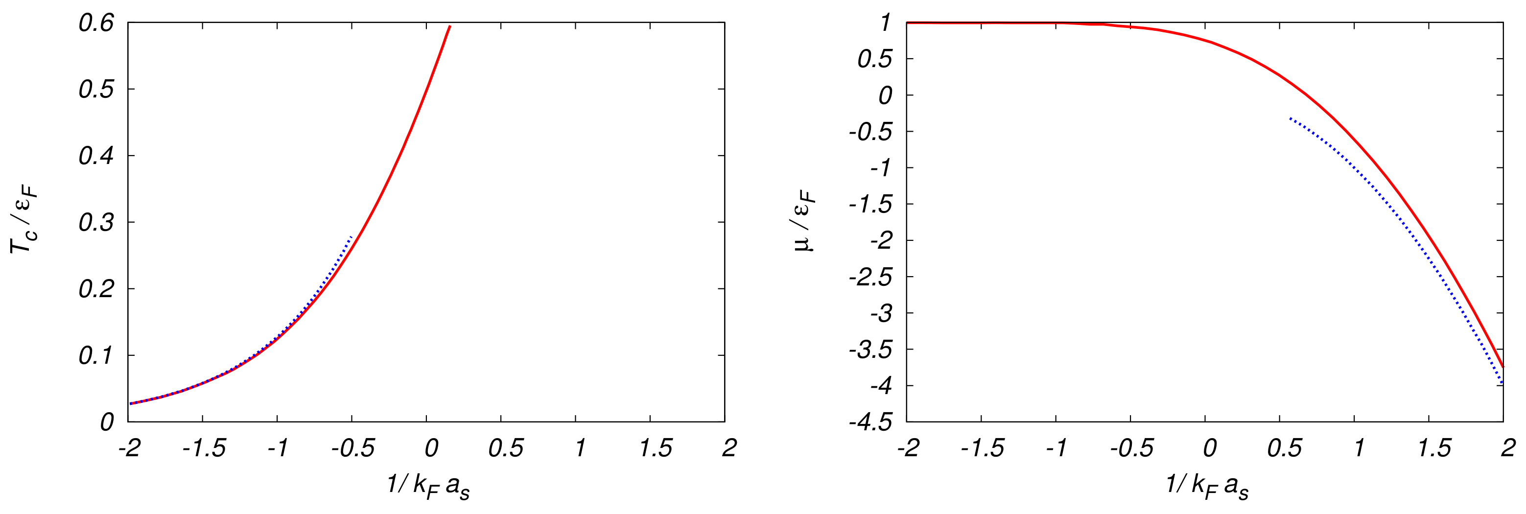
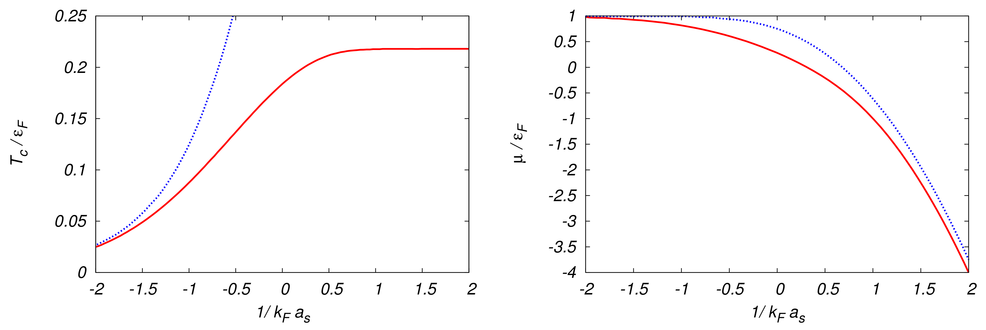
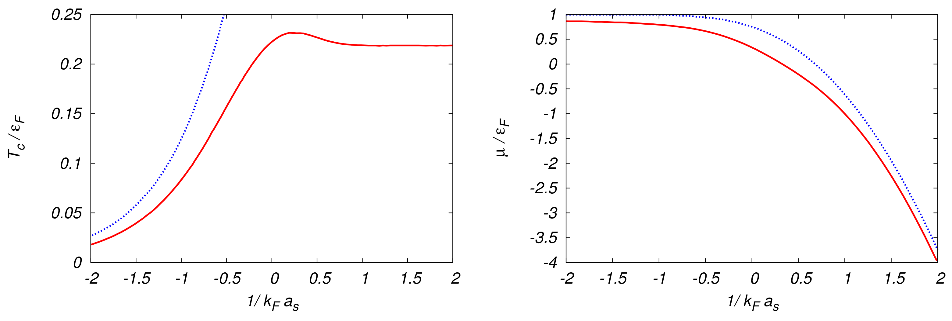
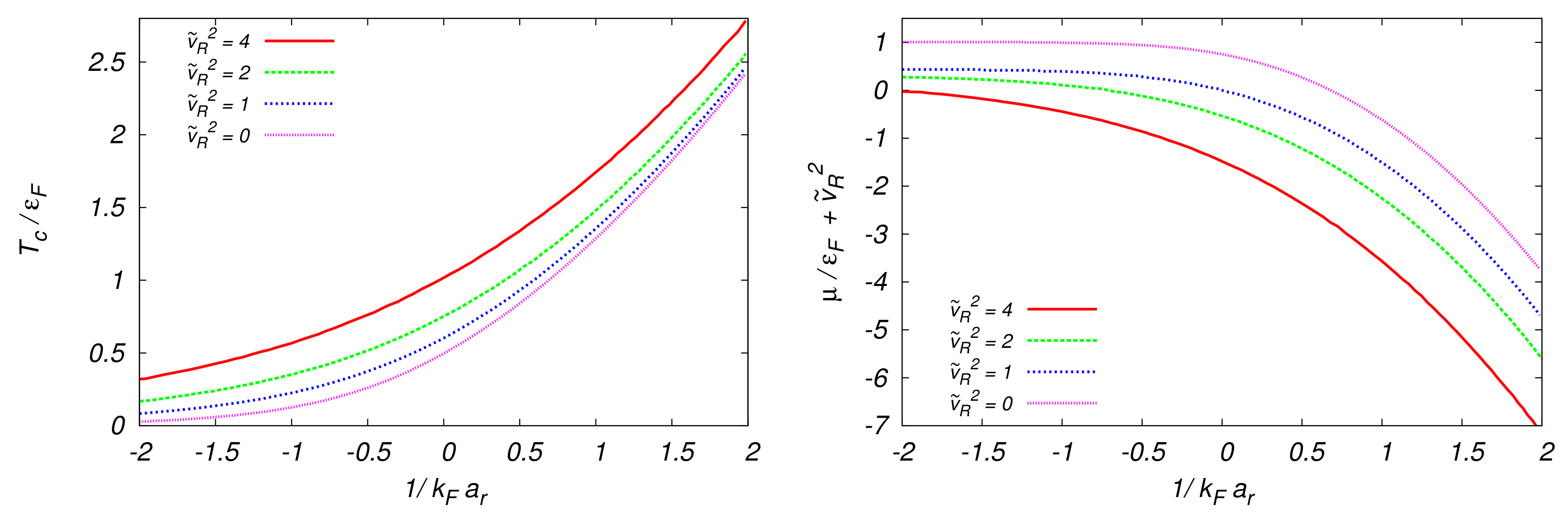
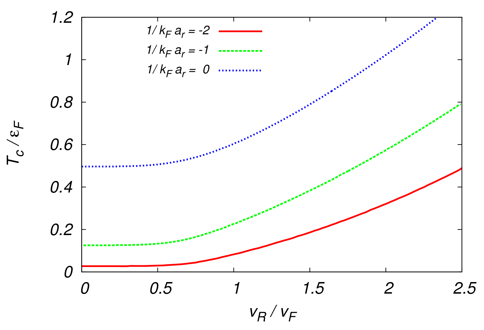
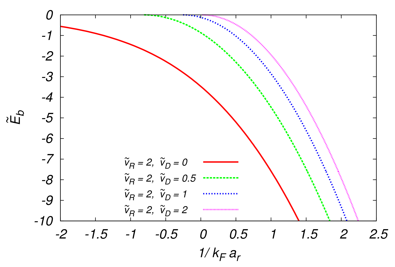
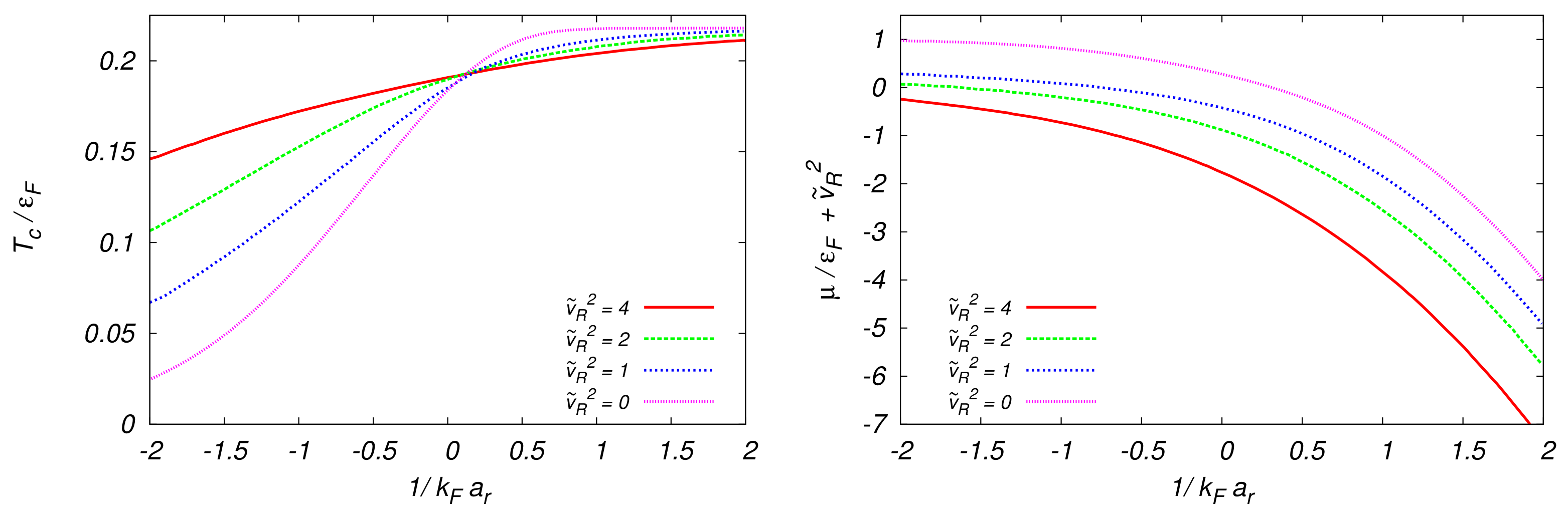
Table A1.
The Riccati-Bessel, , and the Riccati-Neumann, , functions for the first angular momenta .
Table A1.
The Riccati-Bessel, , and the Riccati-Neumann, , functions for the first angular momenta .
The complete solution, for , is then given by a linear superposition of and
with and some coefficients. In the noninteracting problem the solution is fixed by the boundary condition that excludes because of its divergence at the origin, getting
In the interacting case instead, the Schrödinger equation has to be solved also for and then the continuity of the wavefunction and of its first derivative should be imposed at . This is clearly the difficult part of the calculation and an exact solution is known only for a small number of potentials. In Appendix B it has been shown that the scattering solution has the specific form (A10) at large distances. Imposing this behavior to the general solution (A35)
allows us to express the whole solution in terms of the phase shift. As a result, up to an overall prefactor the solution of the radial equation, for , is given by
Interestingly, we notice that the condition for having in Equation (A38) both the contributions of the same order, also in the limit , using Equations (A30) and (A33), is that , which is Equation (25). The expansion of the radial wavefunction (A38) at , at low energy, gives
where is defined in Equation (26), therefore the corresponding wavefunction is
The same form for the wavefunction can be obtained imposing the so-called Bethe-Peierls boundary conditions
One should evaluate the scattering length for a realistic interatomic potential, however in many cases this requires difficult calculations. For this reason it is often convenient to use a simpler pseudo-potential that can reproduce the same scattering amplitude at low energies. Fortunately, the relevant experimental parameter in ultracold atomic physics, tunable by the so-called Feshbach resonance technique, is the scattering length .
- Contact Potentials
The simplest short-range potential is the contact interaction described by a Dirac-delta function in a regularized form or in a bare form.
- Regularized Delta-Funcion
Let us consider the following potential
and write down the s-wave radial equation from Equation (A22)
Recasting the terms we have
For , the s-wave term, we have to solve the following set of equations
The solution of the first equation, as already seen, is
so that the boundary condition can be written as it follows
Using the definition of the scattering length as in Equation (27), with zero effective range, one finds that, in order to model a realistic potential at low energy it is sufficient to use Equation (A42) with
- Bare Delta-Function
Another relevant contact potential is simply
This potential is widely employed in the literature, even though it leads to ultraviolet divergences. The radial equation, in this case, becomes
For the s-wave term we have to solve the following equations
Integrating the second equation we get
Expanding around , only the first two terms survive, and the equation becomes
Using the solution of Equation (A52) which is Equation (A47), we get again the relation
, and dividing by we obtain
where the last term diverges. In order to find a clearer understanding of the relation between g and one has to resort to the formalism of the two-body scattering matrix , see Section 2.1.
Appendix D. Scattering Problem with Spin-Orbit Coupling
In this Appendix we will report the results of Refs. [44,45], using also the same notation. The system of fermions with spin (or pseudo-spin) in the presence of spin–orbit interaction can be characterized by the following single particle Hamiltonian
where and with the usual Pauli matrices for the spin. We will treat later, for simplicity, only the case , and , so a spin–orbit coupling made of a Rashba and a Dresselhaus terms. However some important results can be obtained from the most general Hamiltonian (A57). The Hilbert space of the problem can be expressed as , the product of , the relative motion space and the spin spaces. For clarity different brackets are associated to different spaces, , , , so that the position dependent states of the spin is such that . The same study on two-body problem, seen before, should be done also in this case, always for a spherically symmetric and spin-independent potential , where are the coordinates of the particles. The total two-body Hamiltonian is then
This can be easily separated in the Hamiltonian of the center of mass and Hamiltonian of the relative motion. The latter Hamiltonian is
with the definitions of the relative quantities, . The total momentum is conserved during the scattering process and it can be treated as a constant. A basis of eigenstates for the free Hamiltonian is given by the tensor product of eigenstates of the momentum operator and of spin eigenstates with , labeling the four configurations of two spins, also momentum dependent, which in relative position representation are . Since the momentum part of the eigenfunction is known (plane waves as in the previous case) the eigenproblem can be restricted exclusively to the spin part. In the relative coordinates the Hamiltonian can be decomposed in the following form with
Because of the structure of the operators and Z the single particle Hamiltonian can be written, with , as
The coefficients of the Pauli matrices depend on the specific parameters of the model and linearly by the momentum; for example, should have the form , for some and q model dependent set of parameters. The eigenvalues of are given by
whose asymptotic behavior at large momenta, for the linearity of , and , is given by
For convention is the eigenvector associated to and to . The same problem is identically solved for with the exception of a sign which has to be considered and so the eigenvalues will have the same form but with a different sign in the spin–orbit part of the spectrum. The eigenvectors and are identically assigned and the energies are
With a proper unitary transformation it is always possible to put the Hamiltonian in a diagonal form
The eigenvalues of the total Hamiltonian can be obtained building a basis of eigenstates; with a simple change in the notation , with , this can be done building the basis
The associated eigenvalues are therefore
The four states of spin are labeled by and, for simplicity, we will indicate with , which implicitly depends on , the specific eigenstate of the free Hamiltonian with eigenvalue . To obtain a renormalization relation similar to Equation (40) it is necessary to write the Lippmann–Schwinger equation for the stationary scattering state
Inserting a completeness relation in the position space
The main difficulties in the presence of a SO term are in the Green’s function
The breaking of the rotational symmetry induced by the SO term makes hard the evaluation of the Green’s function and its asymptotic behavior at large distances, therefore, the treatment done before is not easily adaptable to this case. However, as proved in Ref. [45], the scattering amplitude for the two-body problem with SO coupling, in the low energy limit, also for a realistic short range potential (with the range) is
where the state is the singlet spin state and the operator . Specifically the authors of Ref. [44] were able to prove that, for , and , the scattering wavefunction must have the form
This is a natural generalization of the Bethe-Peierls boundary conditions, briefly introduced in (A41). This condition can be exploit to deduce the scattering amplitude of the problem in the same approximations. However to obtain the renormalization condition for a contact potential only the zero energy case is needed, which is shown to be , quite similar to the previous case, with the only difference that should be replaced by the scattering length which now contains also a dependence to the parameters of the SO coupling. Interestingly, also in this case, a bound state near the scattering threshold exists for energies that satisfy
Appendix D.1. Renormalization Condition for a Contact Potential
As done previously, in order to obtain the correct renormalization relation for the contact potential in the presence of a spin–orbit coupling, one can exploit the Lippmann–Schwinger equation and impose that a pseudo-potential reproduces the same scattering amplitude of a realistic potential in the low energy limit. Looking at Equation (A71), the natural choice is to consider a simple contact potential that acts only on the singlet state
The Lippmann–Schwinger equation with the effective potential is given by
It is also useful to remember that the scattering amplitude in terms of the T-matrix is
If two eigenstates of the free Hamiltonian are applied on the right- and on the left-hand sides of Equation (A74), denoting for simplicity by , the scattering amplitude is recovered
Using the zero energy limit for the scattering amplitude , one gets
Simplifying the expression and making explicit the singlet state the obtained relation between the scattering length and the coupling g can be put in the form
We can further simplify this relation using , getting
which, in spherical coordinates, can be written as
Because of the behavior of the eigenvalues shown in Equation (A63) the integrand in the last term of Equation (A80), at large momenta, will have an asymptotic behavior proportional to , therefore, the integral converges to a constant C. We finally get
The constant term can be easily incorporated in the definition of the coupling g, so that the renormalization condition turns to be
The presence of a SO coupling does not alter the form of the renormalization condition for a contact pseudo-potential. The only caution to be taken is to replace with , a scattering length which depends both on the interatomic potential and on the SO term.
References
- Bardeen, J.; Cooper, L.N.; Schrieffer, J.R. Theory of Superconductivity. Phys. Rev. 1957, 106, 162. [Google Scholar] [CrossRef] [Green Version]
- Cooper, L.N. Theory of Superconductivity. Phys. Rev. 1956, 104, 1189. [Google Scholar] [CrossRef]
- Eagles, D.M. Possible Pairing without Superconductivity at Low Carrier Concentrations in Bulk and Thin-Film Superconducting Semiconductors. Phys. Rev. 1969, 186, 456. [Google Scholar] [CrossRef]
- Nozires, P.; Schmitt-Rink, S. Bose condensation in an attractive fermion gas: From weak to strong coupling superconductivity. J. Low Temp. Phys. 1985, 59, 195–211. [Google Scholar] [CrossRef]
- Micnas, R.; Ranninger, J.; Robaszkiewicz, S. Superconductivity in Narrow-Band Systems with Local Nonretarded Attractive Interactions. Rev. Mod. Phys. 1990, 62, 113–171. [Google Scholar] [CrossRef]
- Bednorz, J.G.; Mueller, K.A. Possible high Tc superconductivity in the Ba-La-Cu-O system. Zeitschrift für Physik B 1986, 64, 189–193. [Google Scholar] [CrossRef]
- de Melo, C.A.R.S.; Randeria, M.; Engelbrecht, J.R. Crossover from BCS to Bose superconductivity: Transition temperature and time-dependent Ginzburg-Landau theory. Phys. Rev. Lett. 1993, 71, 3202. [Google Scholar] [CrossRef] [PubMed]
- Davis, K.B.; Mewes, M.O.; Andrews, M.R.; van Druten, N.J.; Durfee, D.S.; Kurn, D.M.; Ketterle, W. Bose-Einstein Condensation in a Gas of Sodium Atoms. Phys. Rev. Lett. 1995, 75, 3969. [Google Scholar] [CrossRef] [Green Version]
- Inouye, S.; Andrews, M.R.; Stenger, J.; Miesner, H.-J.; Stamper-Kurn, D.M.; Ketterle, W. Observation of Feshbach resonances in a BoseEinstein condensate. Nature 1998, 392, 151. [Google Scholar] [CrossRef]
- Courteille, P.; Freeland, R.S.; Heinzen, D.J.; Abeelen, F.A.V.; Verhaar, B.J. Observation of a Feshbach Resonance in Cold Atom Scattering. Phys. Rev. Lett. 1998, 81, 69. [Google Scholar] [CrossRef] [Green Version]
- DeMarco, B.; Jin, D.S. Onset of Fermi Degeneracy in a Trapped Atomic Gas. Science 1999, 285, 1703–1706. [Google Scholar] [CrossRef]
- Loftus, T.; Regal, C.A.; Ticknor, C.; Bohn, J.L.; Jin, D.S. Resonant Control of Elastic Collisions in an Optically Trapped Fermi Gas of Atoms. Phys. Rev. Lett. 2002, 88, 173201. [Google Scholar] [CrossRef] [PubMed] [Green Version]
- Regal, C.A.; Jin, D.S. Measurement of positive and negative scattering lengths in a fermi gas of atoms. Phys. Rev. Lett. 2003, 90, 230404. [Google Scholar] [CrossRef] [Green Version]
- Chin, C.; Grimm, R.; Julienne, P.; Tiesinga, E. Feshbach resonances in ultracold gases. Rev. Mod. Phys. 2010, 82, 1225. [Google Scholar] [CrossRef]
- Regal, C.A.; Greiner, M.; Jin, D.S. Observation of Resonance Condensation of Fermionic Atom Pairs. Phys. Rev. Lett. 2004, 92, 040403. [Google Scholar] [CrossRef] [PubMed] [Green Version]
- Zwierlein, M.W.; Stan, C.A.; Schunck, C.H.; Raupach, S.M.F.; Kerman, A.J.; Ketterle, W. Condensation of Pairs of Fermionic Atoms near a Feshbach Resonance. Phys. Rev. Lett. 2004, 92, 120403. [Google Scholar] [CrossRef] [PubMed] [Green Version]
- Bourdel, T.; Khaykovich, L.; Cubizolles, J.; Chevy, J.Z.F.; Teichmann, M.; Tarruell, L.; Kokkelmans, S.J.J.M.F.; Salomon, C. Experimental Study of the BEC-BCS Crossover Region in Lithium 6. Phys. Rev. Lett. 2004, 93, 050401. [Google Scholar] [CrossRef] [PubMed] [Green Version]
- Kinast, J.; Turlapov, A.; Thomas, J.E.; Chen, Q.; Stajic, J.; Levin, K. Heat Capacity of a Strongly Interacting Fermi Gas. Science 2005, 307, 1296–1299. [Google Scholar] [CrossRef] [Green Version]
- Lin, Y.-J.; Jimnez-Garca, K.; Spielman, I.B. Spinorbit-coupled BoseEinstein condensates. Nature 2011, 471, 83–86. [Google Scholar] [CrossRef]
- Dalibard, J.; Gerbier, F.; Juzeliunas, G.; Ohberg, P. Colloquium: Artificial gauge potentials for neutral atoms. Rev. Mod. Phys. 2011, 83, 1523. [Google Scholar] [CrossRef] [Green Version]
- Wang, P.; Yu, Z.-Q.; Fu, Z.; Miao, J.; Huang, L.; Chai, S.; Zhai, H.; Zhang, J. Spin-Orbit Coupled Degenerate Fermi Gases. Phys. Rev. Lett. 2012, 109, 095301. [Google Scholar] [CrossRef] [Green Version]
- Cheuk, L.W.; Sommer, A.T.; Hadzibabic, Z.; Yefsah, T.; Bakr, W.S.; Zwierlein, M.W. Spin-injection spectroscopy of a spin-orbit coupled Fermi gas. Phys. Rev. Lett. 2012, 109, 095302. [Google Scholar] [CrossRef] [PubMed]
- Bychkov, Y.A.; Rashba, E.I.J. Oscillatory effects and the magnetic susceptibility of carriers in inversion layers. J. Phys. C 1984, 17, 6039. [Google Scholar] [CrossRef]
- Dresselhaus, G. Spin-orbit coupling effects in zinc blende structures. Phys. Rev. 1955, 100, 580. [Google Scholar] [CrossRef]
- Vyasanakere, J.P.; Shenoy, V.B. Bound states of two spin-12 fermions in a synthetic non-Abelian gauge field. Phys. Rev. B 2011, 83, 094515. [Google Scholar] [CrossRef] [Green Version]
- Vyasanakere, J.P.; Zhang, S.; Shenoy, V.B. BCS-BEC crossover induced by a synthetic non-Abelian gauge field. Phys. Rev. B 2011, 84, 014512. [Google Scholar] [CrossRef] [Green Version]
- Gong, M.; Tewari, S.; Zhang, C. BCS-BEC crossover and topological phase transition in 3D spin-orbit coupled degenerate Fermi gases. Phys. Rev. Lett. 2011, 107, 195303. [Google Scholar] [CrossRef] [PubMed] [Green Version]
- Hu, H.; Jiang, L.; Liu, X.; Pu, H. Probing anisotropic superfluidity in atomic Fermi gases with Rashba spin-orbit coupling. Phys. Rev. Lett. 2011, 107, 195304. [Google Scholar] [CrossRef] [PubMed] [Green Version]
- Yu, Z.; Zhai, H. Spin-orbit coupled Fermi gases across a Feshbach resonance. Phys. Rev. Lett. 2011, 107, 195305. [Google Scholar] [CrossRef] [Green Version]
- Iskin, M.; Subasi, A.L. Stability of spin-orbit coupled Fermi gases with population imbalance. Phys. Rev. Lett. 2011, 107, 050402. [Google Scholar] [CrossRef]
- Yi, W.; Guo, G.-C. Phase separation in a polarized Fermi gas with spin-orbit coupling. Phys. Rev. A 2011, 84, 031608. [Google Scholar] [CrossRef] [Green Version]
- Dell’Anna, L.; Mazzarella, G.; Salasnich, L. Condensate fraction of a resonant Fermi gas with spin-orbit coupling in three and two dimensions. Phys. Rev. A 2011, 84, 033633. [Google Scholar] [CrossRef] [Green Version]
- Iskin, M.; Subasi, A.L. Quantum phases of atomic Fermi gases with anisotropic spin-orbit coupling. Phys. Rev. A 2011, 84, 043621. [Google Scholar] [CrossRef] [Green Version]
- Zhou, J.; Zhang, W.; Yi, W. Topological superfluid in a trapped two-dimensional polarized Fermi gas with spin-orbit coupling. Phys. Rev. A 2011, 84, 063603. [Google Scholar] [CrossRef] [Green Version]
- Jiang, L.; Liu, X.-J.; Hu, H.; Pu, H. Rashba spin-orbit-coupled atomic Fermi gases. Phys. Rev. A 2011, 84, 063618. [Google Scholar] [CrossRef]
- Han, L.; de Melo, C.A.R.S. Evolution from BCS to BEC superfluidity in the presence of spin-orbit coupling. Phys. Rev. A 2012, 85, 011606(R). [Google Scholar] [CrossRef] [Green Version]
- Chen, G.; Gong, M.; Zhang, C. BCS-BEC crossover in spin-orbit-coupled two-dimensional Fermi gases. Phys. Rev. A 2012, 85, 013601. [Google Scholar] [CrossRef] [Green Version]
- Zhou, K.; Zhang, Z. Opposite effect of spin-orbit coupling on condensation and superfluidity. Phys. Rev. Lett. 2012, 108, 025301. [Google Scholar] [CrossRef] [PubMed] [Green Version]
- Yang, X.; Wan, S. Phase diagram of a uniform two-dimensional Fermi gas with spin-orbit coupling. Phys. Rev. A 2012, 85, 023633. [Google Scholar] [CrossRef]
- Iskin, M. Vortex line in spin-orbit coupled atomic Fermi gases. Phys. Rev. A 2012, 85, 013622. [Google Scholar] [CrossRef] [Green Version]
- Seo, K.; Han, L.; de Melo, C.A.R.S. Topological phase transitions in ultracold Fermi superfluids: The evolution from Bardeen-Cooper-Schrieffer to Bose-Einstein-condensate superfluids under artificial spin-orbit fields. Phys. Rev. A 2012, 85, 033601. [Google Scholar] [CrossRef] [Green Version]
- He, L.; Huang, X.-G. BCS-BEC crossover in 2D Fermi gases with Rashba spin-orbit coupling. Phys. Rev. Lett. 2012, 108, 145302. [Google Scholar] [CrossRef] [PubMed] [Green Version]
- Dell’Anna, L.; Mazzarella, G.; Salasnich, L. Tuning Rashba and Dresselhaus spin-orbit couplings: Effects on singlet and triplet condensation with Fermi atoms. Phys. Rev. A 2012, 86, 053632. [Google Scholar] [CrossRef] [Green Version]
- Zhang, L.; Zhang, P.; Deng, Y. Modified Bethe-Peierls boundary condition for ultracold atoms with spin-orbit coupling. Phys. Rev. A 2012, 86, 053608. [Google Scholar] [CrossRef] [Green Version]
- Zhang, L.; Deng, Y.; Zhang, P. Scattering and effective interactions of ultracold atoms with spin-orbit interaction. Phys. Rev. A 2013, 87, 053626. [Google Scholar] [CrossRef] [Green Version]
- Cui, J.-X.; Liu, X.-J.; Long, G.L.; Hu, H. Validity of a single-channel model for a spin-orbit-coupled atomic Fermi gas near Feshbach resonances. Phys. Rev. A 2012, 86, 053628. [Google Scholar] [CrossRef] [Green Version]
- He, L.; Huang, X.-G. BCS-BEC crossover in three-dimensional Fermi gases with spherical spin-orbit coupling. Phys. Rev. B 2012, 86, 014511. [Google Scholar] [CrossRef] [Green Version]
- Gong, M.; Chen, G.; Jia, S.; Zhang, C. Searching for Majorana fermions in 2D spin-orbit coupled Fermi superfluids at finite temperature. Phys. Rev. Lett. 2012, 109, 105302. [Google Scholar] [CrossRef]
- Zhang, P.; Zhang, L.; Zhang, W. Interatomic collisions in two-dimensional and quasi-two-dimensional confinements with spin-orbit coupling. Phys. Rev. A 2012, 86, 042707. [Google Scholar] [CrossRef] [Green Version]
- He, L.; Huang, X.G.; Hu, H.; Liu, X.J. BCS-BEC crossover at finite temperature in spin-orbit-coupled Fermi gases. Phys. Rev. A 2013, 87, 053616. [Google Scholar] [CrossRef]
- He, L.; Huang, X.G. Superfluidity and collective modes in Rashba spin–orbit coupled Fermi gases. Ann. Phys. 2013, 337, 163–207. [Google Scholar] [CrossRef] [Green Version]
- Zhou, X.F.; Guo, G.C.; Zhang, W.; Yi, W. Exotic pairing states in a Fermi gas with three-dimensional spin-orbit coupling. Phys. Rev. A 2013, 87, 063606. [Google Scholar] [CrossRef] [Green Version]
- Zhang, K.; Chen, G.; Jia, S. Spin-orbit-induced bound state and molecular signature of the degenerate Fermi gas in a narrow Feshbach resonance. Phys. Rev. A 2013, 88, 013611. [Google Scholar] [CrossRef] [Green Version]
- Caldas, H.; Farias, R.L.S.; Continentino, M. Influence of induced interactions on superfluid properties of quasi-two-dimensional dilute Fermi gases with spin-orbit coupling. Phys. Rev. A 2013, 88, 023615. [Google Scholar] [CrossRef] [Green Version]
- Wu, F.; Guo, G.-C.; Zhang, W.; Yi, W. Unconventional superfluid in a two-dimensional Fermi gas with anisotropic spin-orbit coupling and Zeeman fields. Phys. Rev. Lett. 2013, 110, 110401. [Google Scholar] [CrossRef]
- Wu, F.; Guo, G.-C.; Zhang, W.; Yi, W. Unconventional Fulde-Ferrell-Larkin-Ovchinnikov pairing states in a Fermi gas with spin-orbit coupling. Phys. Rev. A 2013, 88, 043614. [Google Scholar] [CrossRef] [Green Version]
- Liu, X.-J.; Law, K.T.; Ng, T.K.; Lee, P.A. Detecting topological phases in cold atoms. Phys. Rev. Lett. 2013, 111, 120402. [Google Scholar] [CrossRef]
- Salasnich, L. Two-dimensional quasi-ideal Fermi gas with Rashba spin-orbit coupling. Phys. Rev. A 2013, 88, 055601. [Google Scholar] [CrossRef] [Green Version]
- Zhang, W.; Yi, W. Topological Fulde–Ferrell–Larkin–Ovchinnikov states in spin–orbit-coupled Fermi gases. Nature Comm. 2013, 4, 2711. [Google Scholar] [CrossRef] [Green Version]
- Luo, X.; Zhou, K.; Liu, W.; Liang, Z.; Zhang, Z. Fidelity susceptibility and topological phase transition of a two-dimensional spin-orbit-coupled Fermi superfluid. Phys. Rev. A 2014, 89, 043612. [Google Scholar] [CrossRef] [Green Version]
- Wu, F.; Zhang, R.; Deng, T.-S.; Zhang, W.; Yi, W.; Guo, G.-C. BCS-BEC crossover and quantum phase transition in an ultracold Fermi gas under spin-orbit coupling. Phys. Rev. A 2014, 89, 063610. [Google Scholar] [CrossRef] [Green Version]
- Zhou, L.; Cui, X.; Yi, W. Three-component ultracold Fermi gases with spin-orbit coupling. Phys. Rev. Lett. 2014, 112, 195301. [Google Scholar] [CrossRef] [PubMed] [Green Version]
- Zhai, H. Degenerate quantum gases with spin–orbit coupling: A review. Rep. Prog. Phys. 2015, 78, 026001. [Google Scholar] [CrossRef]
- Devreese, J.P.A.; Tempere, J.; de Melo, C.A.R.S. Quantum phase transitions and Berezinskii-Kosterlitz-Thouless temperature in a two-dimensional spin-orbit-coupled Fermi gas. Phys. Rev. A 2015, 92, 043618. [Google Scholar] [CrossRef] [Green Version]
- Wang, J.-K.; Yi, W.; Zhang, W. Two-body physics in quasi-low-dimensional atomic gases under spin–orbit coupling. Front. Phys. 2016, 11, 118102. [Google Scholar] [CrossRef] [Green Version]
- Lee, J.; Kim, D.-H. Induced interactions in the BCS-BEC crossover of two-dimensional Fermi gases with Rashba spin-orbit coupling. Phys. Rev. A 2017, 95, 033609. [Google Scholar] [CrossRef] [Green Version]
- Koinov, Z.; Pahl, S. Spin-orbit-coupled atomic Fermi gases in two-dimensional optical lattices in the presence of a Zeeman field. Phys. Rev. A 2017, 95, 033634. [Google Scholar] [CrossRef] [Green Version]
- Mazziotti, M.V.; Valletta, A.; Raimondi, R.; Bianconi, A. Multigap superconductivity at an unconventional Lifshitz transition in a three-dimensional Rashba heterostructure at the atomic limit. Phys. Rev. B 2021, 103, 024523. [Google Scholar] [CrossRef]
- Martiyanov, K.; Makhalov, V.; Turlapov, A. Observation of a two-dimensional Fermi gas of atoms. Phys. Rev. Lett. 2010, 105, 030404. [Google Scholar] [CrossRef] [PubMed] [Green Version]
- Perali, A.; Pieri, P.; Strinati, G.C. Quantitative comparison between theoretical predictions and experimental results for the BCS-BEC crossover. Phys. Rev. Lett. 2004, 93, 100404. [Google Scholar] [CrossRef] [Green Version]
- Grimm, R.; Ovchinnikov, M.W.A.Y.B. Optical dipole traps for neutral atoms. Adv. At. Mol. Opt. Phys. 2000, 42, 95–170. [Google Scholar]
- Inguscio, M.; Ketterle, W.; Salomon, C. Ultra-Cold Fermi Gases, Proceedings of the International School of Physics “Enrico Fermi”, Course CLXIV; IOS Press: Varenna, Como, Italy, 2007. [Google Scholar]
- Pethick, C.J.; Smith, H. Bose-Einstein Condensation in Dilute Gases; Cambridge University Press: Cambridge, UK, 2008. [Google Scholar]
- Ketterle, W.; Druten, N.J.V. Evaporative cooling of trapped atoms. Adv. At. Mol. Opt. Phys. 1996, 37, 181–236. [Google Scholar]
- Landau, L.D.; Lifshitz, E.M. Quantum Mechanics: Non-relativistic Theory; Course Theoretical Physics Volume 3; Pergamon Press Ltd: Oxford, UK, 1991. [Google Scholar]
- Taylor, J.R. Scattering Theory: The Quantum Theory of Nonrelativistic Collisions; Wiley: Hoboken, NJ, USA, 1972. [Google Scholar]
- Stoof, H.T.C.; Dickerscheid, D.B.M.; Gubbels, K. Ultracold Quantum Fields; Springer: Berlin/Heidelberg, Germany, 2009. [Google Scholar]
- Parish, M.M.; Marchetti, F.M.; Lamacraft, A.; Simons, B.D. Finite temperature phase diagram of a polarised Fermi condensate. Nature Phys. 2007, 3, 124–128. [Google Scholar] [CrossRef] [Green Version]
- Sheey, D.; Radzihovsky, L. BEC–BCS crossover, phase transitions and phase separation in polarized resonantly-paired superfluids. Ann. Phys. 2007, 322, 1790–1924. [Google Scholar] [CrossRef] [Green Version]
- Perali, A.; Pieri, P.; Strinati, G.C.; Castellani, C. Pseudogap and spectral function from superconducting fluctuations to the bosonic limit. Phys. Rev. B 2002, 66, 024510. [Google Scholar] [CrossRef] [Green Version]
- Chen, Q.; Stajic, J.; Tan, S.; Levin, K. BCS–BEC crossover: From high temperature superconductors to ultracold superfluids. Phys. Rep. 2005, 412, 1–88. [Google Scholar] [CrossRef] [Green Version]
- Palestini, F.; Perali, A.; Pieri, P.; Strinati, G.C. Dispersions, weights, and widths of the single-particle spectral function in the normal phase of a Fermi gas. Phys. Rev. B 2012, 85, 024517. [Google Scholar] [CrossRef] [Green Version]
- Khelashvili, A.A.; Nadareishvili, T.P. What is the boundary condition for the radial wave function of the Schrödinger equation? Am. J. Phys. 2011, 79, 668–671. [Google Scholar] [CrossRef]
Figure 1.
Critical temperature and chemical potential at as functions of the inverse of the scattering length . The dashed lines are the analytical results from Equations (99) and (102).

Figure 2.
Critical temperature and chemical potential at within the bosonic approximation. The dashed lines are the mean field results.
Figure 2.
Critical temperature and chemical potential at within the bosonic approximation. The dashed lines are the mean field results.

Figure 3.
Critical temperature and chemical potential at at the Gaussian level. The dashed lines are the mean field results.
Figure 3.
Critical temperature and chemical potential at at the Gaussian level. The dashed lines are the mean field results.

Figure 4.
Critical temperature and chemical potential as functions of y, at the mean field level, for and for different values of .
Figure 4.
Critical temperature and chemical potential as functions of y, at the mean field level, for and for different values of .

Figure 5.
Critical temperature as a function of , at and for some values of .

Figure 6.
Bound state energy for a mixed spin–orbit coupling, keeping fixed and varying . For the binding energy exists only for , in the BEC side, and is exactly the same curve one obtains in the absence of spin–orbit coupling. For pure Rashba (or pure Dresselhaus) the binding energy is always present, also in the BCS side while for any mixed SO coupling there is a threshold value of y for the existence of the binding energy.

Figure 7.
Effective mass ratio , as a function of the coupling , for different values of purely Rashba coupling , from Equations (266) and (267). For only Rashba coupling .

Figure 8.
Critical temperature and chemical potential , at , with the inclusion of the Gaussian fluctuations within the bosonic approximation, for different values of in the purely Rashba case.
Figure 8.
Critical temperature and chemical potential , at , with the inclusion of the Gaussian fluctuations within the bosonic approximation, for different values of in the purely Rashba case.

Publisher’s Note: MDPI stays neutral with regard to jurisdictional claims in published maps and institutional affiliations. |
© 2021 by the authors. Licensee MDPI, Basel, Switzerland. This article is an open access article distributed under the terms and conditions of the Creative Commons Attribution (CC BY) license (https://creativecommons.org/licenses/by/4.0/).
Share and Cite
MDPI and ACS Style
Dell’Anna, L.; Grava, S. Critical Temperature in the BCS-BEC Crossover with Spin-Orbit Coupling. Condens. Matter 2021, 6, 16. https://0-doi-org.brum.beds.ac.uk/10.3390/condmat6020016
AMA Style
Dell’Anna L, Grava S. Critical Temperature in the BCS-BEC Crossover with Spin-Orbit Coupling. Condensed Matter. 2021; 6(2):16. https://0-doi-org.brum.beds.ac.uk/10.3390/condmat6020016
Chicago/Turabian StyleDell’Anna, Luca, and Stefano Grava. 2021. "Critical Temperature in the BCS-BEC Crossover with Spin-Orbit Coupling" Condensed Matter 6, no. 2: 16. https://0-doi-org.brum.beds.ac.uk/10.3390/condmat6020016