Mixtures of Dipolar Gases in Two Dimensions: A Quantum Monte Carlo Study

Abstract

We studied the miscibility of two dipolar quantum gases in the limit of zero temperature. The system under study is composed of a mixture of two Bose gases with dominant dipolar interaction in a two-dimensional harmonic confinement. The dipolar moments are all considered to be perpendicular to the plane, turning the dipolar potential in a purely repulsive and isotropic model. Our analysis is carried out by using the diffusion Monte Carlo method, which allows for an exact solution to the many-body problem within some statistical noise. Our results show that the miscibility between the two species is rather constrained as a function of the relative dipolar moments and masses of the two components. A narrow regime is predicted where both species mix and we introduce an adimensional parameter whose value quite accurately predicts the miscibility of the two dipolar gases.

1. Introduction

Ultracold Bose and Fermi gases have proved to be the best platform for the study of quantum many-body systems [1]. Their versatility and fine tuning of the interatomic interactions allow for the study of many phenomena, which are difficult to attain in real systems. They offer the opportunity of using a laboratory as a quantum simulator of Hamiltonians proposed from theory, which could be difficult to manage using classical computers and algorithms [2,3]. Many of the atoms used to achieve the Bose-Einstein condensate (BEC) state interact among themselves with a contact short-range potential, which depends only on the s-wave scattering length, due to the extreme low density of these gases. However, it has also been possible to cool down to degeneracy gases composed by atoms with a permanent magnetic moment [4]. Exploiting Feshbach resonances, it is proved that the dominant interaction is no more the contact potential but the dipolar interaction between the atomic magnetic moments [5]. The dipolar potential decays as $r^{-3}$ and thus the interaction effects become fundamental in the properties of the gas.

First experiments showing dipolar effects were carried out with Cr, with a magnetic moment $\mu =6{\mu }_B$ [5]. In the last years, two more candidates have joined this class of materials, Dy [6] with $\mu =10{\mu }_B$ and Er [7] with $\mu =7{\mu }_B$, significantly widening the possibilities for observing the two main features of these systems: anisotropy and slow-decaying two-body interactions [8]. The different interaction between side-by-side moments (repulsive) and head-to-tail ones (attractive) leads to the formation of self-bound liquid drops if the number of atoms is above a threshold known as critical atom number [9]. By changing the total scattering length of the system, one can see how the critical atom number increases when the scattering length also increases [10]. Under proper harmonic confinement, and when the number of atoms is large enough, one observes that the system arranges in drops forming a linear array, if the trapping is cigar-shaped, and a triangular one is in a plane, it has a pancake form. Interestingly, these patterns emulate a crystal, but where every site is not monoatomic but occupied by a multiparticle drop. Recent experimental work claims that these solid-like patterns show coherence and thus are examples of the pursued supersolid state of matter [11,12,13].

The field of ultracold dipolar gases has entered an even more rich landscape with the realization of Er-Dy mixtures [14,15,16]. The interplay between the two dipolar species opens new scenarios like the formation of mixed dipolar drops and the possible stability of mixed supersolids, with arrays composed by single-species drops or mixed drops. A key ingredient in this discussion is the miscibility of the two species since inmiscibility would hinder the observation of these new intriguing phases. Recent measures on this system show that both components tend to be phase separated, both due to the gravitational sag originated by the different masses of Er and Dy and by an overall repulsive interaction between both condensates [16]. Dipolar mixtures in three dimensions have also been theoretically studied, focusing on the miscibility of both species [17,18,19], the structure of emerging vortices under rotation [20,21], and the formation of mixed dipolar drops [22,23].

Dipolar mixtures add long-range and anisotropy in the field of quantum mixtures. The case of short-range or contact repulsive interactions in the mixtures is well understood, both from theory and experiment [24,25,26,27,28,29,30,31,32]. The miscibility criterion when the mixture is harmonically confined was analyzed in Refs. [33,34], concluding that in dilute mixtures the criterium for the bulk also works quite well in the confined case.

In the present work, we use the ab initio diffusion Monte Carlo (DMC) method to study a mixture of two dipolar Bose gases harmonically confined in two dimensions (2D). In our analysis, we assume that all the dipoles are oriented perpendicularly to the plane and thus interact with a fully repulsive $1/r^3$ potential. A single dipolar gas in the same conditions was studied some time ago with DMC but in an extended configuration, free from confinement. It was shown that the gas becomes a triangular crystal when the density increases [35]. If the dipoles are not perpendicular to the plane but tilted at a certain angle, the interaction becomes anisotropic and, beyond a certain critical angle, it collapses. That anisotropy produces a rich diagram, with a stable stripe phase [36], which is indeed a supersolid or superstripe that suffers a Berezinskii–Kostrelitz–Thouless phase transition at finite temperature [37].

As a function of the ratio between both the dipolar moments and the masses of the two species in the mixture, we analyze the miscibility of the two gases. Our results show that both species are miscible only in a restricted area in the dipolar moment, a mass ratio plane where both ratios are close to one. In the majority of situations that we analyzed, we observe that the two confined gases do not mix: one species remains in the center and the second goes to the surface. If the trap is deformed, we observe that in some cases the external component appears in two separated blobs, separated by the inner species. Finally, we particularize our study to the Er-Dy mixture and predict that both species do not mix, in agreement with available experimental data.

The rest of the paper is organized as follows. In Section 2, we discuss the quantum Monte Carlo methods used in our study and the miscibility criterion that accounts well for the phase diagram. In Section 3, we present the results obtained for both isotropic and anisotropic traps and analyze the particular case of an Er-Dy mixture, which is the one observed recently in experiments. Finally, Section 4 comprises the summary of the main results and the conclusions of our work.

2. Quantum Monte Carlo Methods

2.1. Hamiltonian

The object of study of this work are two-component dipolar bosonic mixtures at zero temperature, in a purely two dimensional geometry. We consider that all the magnetic moments are perpendicular to the plane and the gas is confined by either an isotropic harmonic trap or an anisotropic one. The dipole–dipole interaction (DDI) potential between two identical particles is given by

$$V_{dd}\left(\mathbf{r}\right)=\frac{C_{dd}}{4\pi }\frac{{\widehat{\mathbf{p}}}_1·{\widehat{\mathbf{p}}}_2-3({\widehat{\mathbf{p}}}_1·\widehat{\mathbf{r}})({\widehat{\mathbf{p}}}_2·\widehat{\mathbf{r}})}{r^3},$$

(1)

with $C_{dd}={\mu }_0{\mu }^2$, ${\mu }_0$ being the magnetic permeability of free space and $\mu$ the particle’s magnetic moment. ${\widehat{\mathbf{p}}}_1$ and ${\widehat{\mathbf{p}}}_2$ are the vectors pointing in the direction of the dipole’s moment of particles 1 and 2, respectively, and $\widehat{\mathbf{r}}=\mathbf{r}/r$ is the unit position vector. In our case, with the particles confined to the $xy$ plane and polarized parallel to the z axis, the interaction is always isotropic and repulsive,

$$V_{dd}\left(\mathbf{r}\right)=V_{dd}\left(r\right)=\frac{C_{dd}}{4\pi }\frac{1}{r^3}.$$

(2)

This is the dipolar potential of a purely 2D system and it corresponds to a pancake geometry where the transverse confinement has an energy $\hslash \omega \gg E/N$, with $E/N$ being the interaction energy per particle. In other words, the oscillator length of the transverse confinement is assumed to be much smaller than the mean interparticle distance. If this is not the case, one needs to include a short range repulsive (contact) interaction that stabilizes the system [10,38]. The mixture is confined by a 2D harmonic oscillator (ho) potential, which in the isotropic case is given by

$$V_{ho}\left(r_i\right)=\frac{1}{2}m{\omega }^2{r}_i^2,$$

(3)

where m is the mass of the particle, $\omega$ is the ho’s trapping frequency, and $r_i$ is the particle’s distance to the origin, which matches the center of the trap. The full Hamiltonian of the system is then given by

$$\begin{array}{c}\hfill H\left(\mathbf{R}\right)=-\frac{{\hslash }^2}{2m_1}{\nabla }_{{\mathbf{R}}_1}^2-\frac{{\hslash }^2}{2m_2}{\nabla }_{{\mathbf{R}}_2}^2+\frac{1}{2}{m}_1{\omega }_1^2\sum _{i=1}^{N_1}{r}_i^2+\frac{1}{2}{m}_2{\omega }_2^2\sum _{k=N_1+1}^N{r}_k^2\\ \hfill +\frac{{\mu }_0{\mu }_1^2}{4\pi }\sum _{i=1}^{N_1-1}\sum _{j=i+1}^{N_1}\frac{1}{r_{ij}^3}+\frac{{\mu }_0{\mu }_2^2}{4\pi }\sum _{i=N_1+1}^{N-1}\sum _{j=i+1}^N\frac{1}{r_{ij}^3}+\frac{{\mu }_0{\mu }_1{\mu }_2}{4\pi }\sum _{i=1}^{N_1}\sum _{j=N_1+1}^N\frac{1}{r_{ij}^3},\end{array}$$

(4)

with $N=N_1+N_2$, $N_1$ and $N_2$ being the number of particles of each type in our mixture, and $m_1$ and $m_2$ the corresponding mass of the particles. In order to simplify Equation (4), we have used $\mathbf{R}=\{{\mathbf{r}}_1,{\mathbf{r}}_2,\cdots ,{\mathbf{r}}_N\}$ as the whole coordinate set such that ${\sum }_i{\nabla }_i^2={\nabla }_{\mathbf{R}}^2$. Finally, ${\omega }_1$ and ${\omega }_2$ are the trapping frequencies and ${\mu }_1$ and ${\mu }_2$ are the magnetic dipole moments of type 1 and 2 particles, respectively, with ${\mathbf{r}}_{ij}={\mathbf{r}}_i-{\mathbf{r}}_j$.

As in previous studies [35], we use dipolar units (for species 1),

$$r_0=\frac{m_1{C}_{dd}^{\left(11\right)}}{4\pi {\hslash }^2}=\frac{m_1{\mu }_0{\mu }_1^2}{4\pi {\hslash }^2}\&E_0=\frac{{\hslash }^2}{m_1{r}_0^2},$$

(5)

with $r_0$ and $E_0$ being the units of distance and energy, respectively. Then, in these units, the Hamiltonian is written as

$$\begin{array}{c}\hfill H\left({\mathbf{R}}^{*}\right)=-\frac{1}{2}{\nabla }_{{\mathbf{R}}_1^{*}}^2-\frac{1}{2}\frac{m_1}{m_2}{\nabla }_{{\mathbf{R}}_2^{*}}^2+\frac{1}{2}{A}_1\sum _{i=1}^{N_1}{r}_i^{*,2}+\frac{1}{2}{A}_2\sum _{k=N_1+1}^N{r}_k^{*,2}\\ \hfill +\sum _{i=1}^{N_1}\sum _{j=i+1}^{N_1-1}\frac{1}{r_{ij}^{*,3}}+{\left(\frac{{\mu }_2}{{\mu }_1}\right)}^2\sum _{i=N_1+1}^{N-1}\sum _{j=i+1}^N\frac{1}{r_{ij}^{*,3}}+\frac{{\mu }_2}{{\mu }_1}\sum _{i=1}^{N_1}\sum _{j=N_1+1}^N\frac{1}{r_{ij}^{*,3}},\end{array}$$

(6)

where the superscript ’${}^{*}$‘ denotes the use of normalized units $r^{*}=r/r_0$. The strength of the harmonic confinement in both species is

$$A_1=\frac{m_1^2{\omega }_1^2{r}_0^4}{{\hslash }^2}={\left(\frac{r_0}{l_1}\right)}^4\&A_2=\frac{m_1{m}_2{\omega }_2^2{r}_0^4}{{\hslash }^2}=\frac{m_1}{m_2}{\left(\frac{r_0}{l_2}\right)}^4=\frac{m_2{\omega }_2^2}{m_1{\omega }_1^2}{A}_1,$$

(7)

with $l_1=\sqrt{\hslash /m_1{\omega }_1}$ and $l_2=\sqrt{\hslash /m_2{\omega }_2}$ being the harmonic oscillator lengths.

We have also explored the effects induced by an anisotropic confinement. The Hamiltonian in this case is

$$\begin{array}{c}\hfill H\left({\mathbf{R}}^{*}\right)=-\frac{1}{2}{\nabla }_{{\mathbf{R}}_1^{*}}^2-\frac{1}{2}\frac{m_1}{m_2}{\nabla }_{{\mathbf{R}}_2^{*}}^2+\frac{A_{x,1}}{2}\sum _{i=1}^{N_1}{x}_i^{*,2}+\frac{A_{x,2}}{2}\sum _{k=N_1+1}^N{x}_k^{*,2}+\frac{A_{y,1}}{2}\sum _{i=1}^{N_1}{y}_i^{*,2}\\ \hfill +\frac{A_{y,2}}{2}\sum _{k=N_1+1}^N{y}_k^{*,2}+\sum _{i=1}^{N_1-1}\sum _{j=i+1}^{N_1}\frac{1}{r_{ij}^{*,3}}+{\left(\frac{{\mu }_2}{{\mu }_1}\right)}^2\sum _{i=N_1+1}^{N-1}\sum _{j=i+1}^N\frac{1}{r_{ij}^{*,3}}+\frac{{\mu }_2}{{\mu }_1}\sum _{i=1}^{N_1}\sum _{j=N_1+1}^N\frac{1}{r_{ij}^{*,3}},\end{array}$$

(8)

with

$$\begin{array}{ccc}\hfill A_{x,1}& =\frac{m_1^2{\omega }_{x,1}^2{r}_0^4}{{\hslash }^2}={\left(\frac{r_0}{l_{x,1}}\right)}^4,A_{x,2}\hfill & \hfill =\frac{m_1{m}_2{\omega }_{x,2}^2{r}_0^4}{{\hslash }^2}=\frac{m_1}{m_2}{\left(\frac{r_0}{l_{x,2}}\right)}^4=\frac{m_2{\omega }_{x,2}^2}{m_1{\omega }_{x,1}^2}{A}_{x,1}\\ \hfill A_{y,1}& =\frac{m_1^2{\omega }_{y,1}^2{r}_0^4}{{\hslash }^2}={\left(\frac{r_0}{l_{y,1}}\right)}^4,A_{y,2}\hfill & \hfill =\frac{m_1{m}_2{\omega }_{y,2}^2{r}_0^4}{{\hslash }^2}=\frac{m_1}{m_2}{\left(\frac{r_0}{l_{y,2}}\right)}^4=\frac{m_2{\omega }_{y,2}^2}{m_1{\omega }_{y,1}^2}{A}_{y,1}.\end{array}$$

(9)

The oscillator lengths are now: $l_{x,1}=\sqrt{\hslash /m_1{\omega }_{x,1}}$, $l_{x,2}=\sqrt{\hslash /m_2{\omega }_{x,2}}$, $l_{y,1}=\sqrt{\hslash /m_1{\omega }_{y,1}}$, and $l_{y,2}=\sqrt{\hslash /m_2{\omega }_{y,2}}$.

To reduce the number of variables of our numerical simulations, we assume that both types of particles are under the presence of the same harmonic potential, with strengths $A_x$ in the x-direction and $A_y$ in the y-direction. Therefore, $m_1{\omega }_{x,1}^2=m_2{\omega }_{x,2}^2$ and $m_1{\omega }_{y,1}^2=m_2{\omega }_{y,2}^2$, ${\omega }_{x,\alpha }$ and ${\omega }_{y,\alpha }$ are the confinement frequencies for type $\alpha$ particles along the x and y axes, respectively. This also applies to the isotropic case, where we consider $A_1=A_2$ via the use of different confinement frequencies verifying $m_1{\omega }_1^2=m_2{\omega }_2^2$.

2.2. Diffusion Monte Carlo

The main theoretical tool used in this work is the diffusion Monte Carlo (DMC) method, which finds the ground-state energy of a many-particle system by propagating the imaginary-time Schrödinger equation exploiting the similarities with a diffusion process.

The time-dependent Schrödinger equation associated to a system of N particles, written in imaginary time $\tau =it/\hslash$, is

$$-\frac{\partial |\mathrm{\Psi }\left(\tau \right)⟩}{\partial \tau }=(\widehat{H}-E_T)\left|\mathrm{\Psi }\right(\tau )⟩.$$

(10)

Its solution is given by $\left|\mathrm{\Psi }\right(\tau )⟩=\widehat{U}(\tau ,0)\left|\mathrm{\Psi }\right(0)⟩$, where $\widehat{U}(\tau ,0)=\exp [-(\widehat{H}-E_T)\tau )]$ is the imaginary-time evolution operator and $E_T$ is the reference energy. Projecting in coordinate space,

$$\mathrm{\Psi }(\mathbf{R},\tau )=\int d{\mathbf{R}}^{\prime }G(\mathbf{R},{\mathbf{R}}^{\prime },\tau )\mathrm{\Psi }(\mathbf{R},0),$$

(11)

with $⟨\mathbf{R}|\widehat{U}(\tau ,0)|{\mathbf{R}}^{\prime }⟩\equiv G(\mathbf{R},{\mathbf{R}}^{\prime },\tau )$ being the Green function and $G(\mathbf{R},{\mathbf{R}}^{\prime },0)=\delta (\mathbf{R}-{\mathbf{R}}^{\prime })$ its initial condition. The above integral (11) is in principle intractable due to the non-commutativity of the kinetic and potential operators that appear in the Green function. As we will shortly discuss, we may avoid this by computing short-time approximations for $G(\mathbf{R},{\mathbf{R}}^{\prime },\tau )$ and using the convolution property of Equation (11).

As in many Monte Carlo simulations, it is convenient to introduce importance sampling to reduce the variance to a manageable level. In DMC, this is carried out by solving the Schrödinger equation for the wave function

$$f(\mathbf{R},\tau )\equiv \mathrm{\Psi }(\mathbf{R},\tau ){\mathrm{\Psi }}_T\left(\mathbf{R}\right),$$

(12)

where ${\mathrm{\Psi }}_T\left(\mathbf{R}\right)$ is a time-independent trial wave function, which in our case is previously optimized using the variational Monte Carlo (VMC) method [39], and whose specific form for the present problem will be discussed in Section 2.3. ${\mathrm{\Psi }}_T$ acts as a guiding wave function, which drives the system away from regions of the phase space where the interatomic potential is strongly repulsive, or even divergent, and increases the sampling of regions where the wave function is expected to be large. With that, the Schrödinger equation may be rewritten as

$$-\frac{\partial f(\mathbf{R},\tau )}{\partial \tau }=({\widehat{O}}_K+{\widehat{O}}_D+{\widehat{O}}_B)f(\mathbf{R},\tau ),$$

(13)

where

$${\widehat{O}}_K=-D{\nabla }_R^2,{\widehat{O}}_D=D\left[({\nabla }_R·\mathbf{F}\left(\mathbf{R}\right))+\mathbf{F}\left(\mathbf{R}\right)·{\nabla }_{\mathbf{R}}\right]\&{\widehat{O}}_B=E_L\left(\mathbf{R}\right)-E_T$$

(14)

are known as the kinetic, drift, and branching operators, respectively. $D={\hslash }^2/\left(2m\right)$ and $E_L\left(\mathbf{R}\right)=\frac{H\left(\mathbf{R}\right){\mathrm{\Psi }}_T\left(\mathbf{R}\right)}{{\mathrm{\Psi }}_T\left(\mathbf{R}\right)}$ is the local energy. The kinetic term, which gives DMC its name, is the same as a classical diffusion operator, ${\widehat{O}}_D$ guides the diffusion process, and, as we will see, ${\widehat{O}}_B$ promotes lower energy configurations and removes higher energy ones. Then, in a formal sense, this leads to

$$f(\mathbf{R},\tau )=\int d{\mathbf{R}}^{\prime }G(\mathbf{R},{\mathbf{R}}^{\prime },\tau )f(\mathbf{R},0),$$

(15)

with $G(\mathbf{R},{\mathbf{R}}^{\prime },0)=\delta (\mathbf{R}-{\mathbf{R}}^{\prime })$. Specifically, $G(\mathbf{R},{\mathbf{R}}^{\prime },\tau )=\exp [-({\widehat{O}}_K+{\widehat{O}}_D+{\widehat{O}}_B)\tau ]$. The situation is formally the same as in the non-importance sampling case, as these three operators do not commute, and thus a short-time approximation needs to be used. In fact, the Green functions associated to each operator can be calculated in the limit $\tau \to 0$.

The kinetic part, $G_K(\mathbf{R},{\mathbf{R}}^{\prime },\tau )$, is straightforwardly obtained by using the completeness relation of the momentum basis and gaussian integration, leading to

$$G_K(\mathbf{R},{\mathbf{R}}^{\prime },\tau )=⟨\mathbf{R}\left|e^{-{\widehat{O}}_K\tau }\right|{\mathbf{R}}^{\prime }⟩={\left(4\pi D\tau \right)}^{-dN/2}\exp \left[-\frac{{(\mathbf{R}-{\mathbf{R}}^{\prime })}^2}{4D\tau }\right],$$

(16)

with d the dimension of the system. Concerning the drift term, it verifies [40]

$$G_D(\mathbf{R},{\mathbf{R}}^{\prime },\tau )=⟨\mathbf{R}\left|e^{-{\widehat{O}}_D\tau }\right|{\mathbf{R}}^{\prime }⟩=\delta (\mathbf{R}-{\mathcal{R}}^{\prime }\left(\tau \right)),$$

(17)

where ${\mathcal{R}}^{\prime }\left(\tau \right)$ is deterministically calculated by solving the differential equation

$$\frac{d\mathcal{R}\left(\tau \right)}{d\tau }=D\mathbf{F}\left(\mathcal{R}\left(\tau \right)\right),$$

(18)

with the initial condition $\mathcal{R}\left(0\right)=\mathbf{R}$. Finally, the Green function associated to the branching term is easily obtained as

$$G_B(\mathbf{R},{\mathbf{R}}^{\prime },\tau )=⟨\mathbf{R}\left|e^{-(E_L\left(\mathbf{R}\right)-E_T)\tau )}\right|{\mathbf{R}}^{\prime }⟩=e^{-(E_L\left(\mathbf{R}\right)-E_T)\tau }\delta (\mathbf{R}-{\mathbf{R}}^{\prime }).$$

(19)

One might then be tempted to approximate $G(\mathbf{R},{\mathbf{R}}^{\prime },\Delta \tau )$ for small $\Delta \tau$ in terms of $G_K$, $G_D$ and $G_B$ linearly in $\Delta \tau$ as

$$G(\mathbf{R},{\mathbf{R}}^{\prime },\Delta \tau )=⟨\mathbf{R}\left|e^{-({\widehat{O}}_K+{\widehat{O}}_D+{\widehat{O}}_B)\Delta \tau }\right|{\mathbf{R}}^{\prime }⟩=⟨\mathbf{R}\left|e^{-{\widehat{O}}_K\Delta \tau }{e}^{-{\widehat{O}}_D\Delta \tau }{e}^{-{\widehat{O}}_B\Delta \tau }\right|{\mathbf{R}}^{\prime }⟩+\mathcal{O}(\Delta {\tau }^2).$$

(20)

However, that would lead to a strong dependence with $\Delta \tau$, which would require to use very small time-steps. Instead, we use an approximation accurate to order $\Delta {\tau }^2$ given by

$$G(\mathbf{R},{\mathbf{R}}^{\prime },\Delta \tau )=⟨\mathbf{R}\left|e^{-{\widehat{O}}_B\Delta \tau /2}{e}^{-{\widehat{O}}_D\Delta \tau /2}{e}^{-{\widehat{O}}_K\Delta \tau }{e}^{-{\widehat{O}}_D\Delta \tau /2}{e}^{-{\widehat{O}}_B\Delta \tau /2}\right|{\mathcal{R}}^{\prime }⟩+\mathcal{O}(\Delta {\tau }^3),$$

(21)

which gives name to the method known as quadratic diffusion Monte Carlo [41,42], which is used throughout this work.

Having discussed the formal concepts associated with the DMC method, let us then comment how it is applied in practice. In order to evolve the system, one represents it using sets of coordinates $\{{\mathbf{R}}_1,{\mathbf{R}}_2,\cdots ,{\mathbf{R}}_{N_w}\}$ known as walkers, each one being a configuration of the N-particle system, which is to be propagated separately. One then makes use of the approximation (Equation (21)), with each operator in this expression applied in the same order each time-step.

The diffusion operator is straightforwardly applied, as one can use the Box–Muller algorithm to sample from the desired Gaussian distribution. The drift operator $\exp (-{\widehat{O}}_D\Delta \tau /2)$ is deterministic, and requires solving Equation (18) exactly to order $\Delta {\tau }^2$. We do this by using the second-order Runge–Kutta method. Finally, the branching operator kills or reproduces walkers based on the difference between their local energy $E_L$ and the reference energy $E_T$. This way, we promote the configurations with the lowest energy and remove the ones with a higher energy. To implement the branching term, the number of copies of a given walker is calculated as

$$N_{\mathrm{sons}}=\left[\exp \left\{-\left(\frac{E_L\left(\mathbf{R}\right)+E_L\left({\mathbf{R}}^{\prime }\right)}{2}-E_T\right)\tau \right\}+\eta \right],$$

(22)

where $\eta$ is sampled from the uniform probability distribution $U[0,1)$, $[\cdots ]$ denotes the integer part, and $\mathbf{R}$, ${\mathbf{R}}^{\prime }$ are walkers at two successive times.

In a DMC simulation, one fixes the time-step $\Delta \tau$, the desired number of walkers $N_w$, and chooses a guiding wave function whose parameters are previously optimized using the VMC method. Then, after each time-step, a new set of walkers is obtained and after every block $E_T$ is updated to be the average local energy of the previous set. Approaching the limit $\tau \to \infty$, we get the ground-state energy $E_0$ as a mean of the local energies of the walkers set. It is important to remark, however, that this estimate is only exact in the limits $\Delta \tau \to 0$ and $1/N_w\to 0$. This way, different simulations approaching these two limits have to be made in order to obtain the result as an extrapolation to such limits. This is the method used throughout this work, and any result shown in Section 3 has been obtained by an initial optimization of the trial wave function via VMC, followed by its use as a guiding function in DMC, and the check for the optimum $N_w$ and $\Delta \tau$ values.

Finally, to conclude this discussion on the DMC method we briefly describe the estimation of observables. In a DMC simulation we sample the mixed wave function $f(\mathbf{R},\tau )=\mathrm{\Psi }(\mathbf{R},\tau ){\mathrm{\Psi }}_T\left(\mathbf{R}\right)$ as $\tau \to \infty$, such that $f(\mathbf{R},\tau \to \infty )\to {\varphi }_0\left(\mathbf{R}\right){\mathrm{\Psi }}_T\left(\mathbf{R}\right)$, where ${\varphi }_0$ is the exact ground state wave function, in a process known as mixed estimation. In case the operator being estimated is the Hamiltonian or commutes with it, this leads to an exact estimation within some statistical errors. However, for other operators, such as the potential energy or the density profile, the estimation is biased in a way that makes it difficult to assess a priori. The simplest way to approximately correct this bias is to use an extrapolated estimator, which makes use of both mixed (DMC) and variational (VMC) results. This result, however, is still biased in an unknown way as it still depends on the trial wave function. The solution to definitely eliminate that bias is by means of the pure estimation, a technique based on forward walking, which we use throughout this work as implemented in Ref. [43].

2.3. The Trial Wave Functions

As we have discussed in the previous section, a reasonable choice for the ground-state wave function is necessary to guide the diffusion process in DMC. The usual approach, and the one taken in this work, is to use the VMC method to optimize the trial wave function before using it in the DMC method.

Our system is a bosonic one, so the wave function must be symmetric with respect to exchange of particles. We include one- and two-body correlation factors in the usual Bijl–Jastrow form [44],

$$\mathrm{\Psi }\left(\mathbf{R}\right)={\psi }_1\left(\mathbf{R}\right){\psi }_2\left(\mathbf{R}\right),$$

(23)

with

$${\psi }_1\left(\mathbf{R}\right)=exp\left(\sum _{i=1}^{N_1}{u}_1^{\left(1\right)}\left(r_i\right)+\sum _{i=N_1+1}^N{u}_1^{\left(2\right)}\left(r_i\right)\right)$$

(24)

the one-body terms and

$${\psi }_2\left(\mathbf{R}\right)=exp\left(\sum _{i=1}^{N_1-1}\sum _{j=i+1}^{N_1}{u}_2^{\left(11\right)}\left(r_{ij}\right)+\sum _{i=N_1+1}^{N-1}\sum _{j=i+1}^N{u}_2^{\left(22\right)}\left(r_{ij}\right)+\sum _{i=1}^{N_1}\sum _{j=N_1+1}^N{u}_2^{\left(12\right)}\left(r_{ij}\right)\right)$$

(25)

the two-body ones. The one-body terms $u_1^{\left(\alpha \right)}\left(r\right)$ are chosen as the analytical solutions (Gaussian functions) of a single particle confined by the harmonic trap, either isotropic or anisotropic. These terms are Gaussian functions and depend on the specific species of the mixture. For the two-body terms associated to the interatomic dipolar potentials, we use the short-distance approximation of the solution for two untrapped interacting dipoles [45],

$$u_2^{\left(\alpha \beta \right)}\left(r_{ij}\right)=-\sqrt{\frac{2{\mu }_{\alpha \beta }{C}_{dd}^{\left(\alpha \beta \right)}}{4\pi {\hslash }^2}}\frac{2}{\sqrt{r_{ij}}},$$

(26)

with ${\mu }_{\alpha \beta }=m_{\alpha }{m}_{\beta }/(m_{\alpha }+m_{\beta })$ the reduced mass of an $\alpha -\beta$ pair, and $C_{dd}^{\left(\alpha \beta \right)}={\mu }_0{\mu }_{\alpha }{\mu }_{\beta }$. Wave functions (26) are too repulsive for intermediate and large inter-particle distances. Therefore, we match Equation (26) with softer $u_2$ terms for $r_{ij}^{*}=R_{\mathrm{cut}}^{\left(\alpha \beta \right)}$,

$$u_2^{\left(\alpha \beta \right)}\left(r_{ij}^{*}\right)=c_2^{\left(\alpha \beta \right)}-\frac{c_3^{\left(\alpha \beta \right)}}{r_{ij}^{*}},$$

(27)

with $c_2^{\left(\alpha \beta \right)}$, $c_3^{\left(\alpha \beta \right)}$, and $R_{\mathrm{cut}}^{\left(\alpha \beta \right)}$ constants for each type of $\alpha -\beta$ interaction, such that the wave function and its first derivative are continuous at $r_{ij}^{*}=R_{\mathrm{cut}}^{\left(\alpha \beta \right)}$. This is then introduced in the VMC code with $R_{\mathrm{cut}}^{\left(\alpha \beta \right)}=r_p^{\left(\alpha \beta \right)}{A}_1^{-1/4}$ in the isotropic case, with $r_p^{\left(\alpha \beta \right)}$ being the only free variational parameters with respect to which the trial wave function is optimized. In the presence of an anisotropic harmonic potential, this is adapted considering $r_p^{\left(\alpha \beta \right)}\sqrt{A_x^{-1/4}{A}_y^{-1/4}}$ as a more convenient choice for the matching distance.

2.4. The Miscibility Criterion

The miscibility in Bose–Bose mixtures is determined by the parameter $\Delta$,

$$\Delta =\frac{g_{11}{g}_{22}}{g_{12}^2}-1,$$

(28)

a criteria derived from the mean-field treatment of bulk mixtures [34]. Equation (28) classifies the behavior of the mixtures: $\Delta >0$ signals miscibility, $\Delta <0$ phase separation, and $\Delta =0$ the critical value separating both regimes.

In three dimensions, the interaction strengths in Equation (28) read

$$g_{\alpha ,\beta }=\frac{2\pi {\hslash }^2{a}_{\alpha \beta }}{{\mu }_{\alpha \beta }},$$

(29)

with ${\mu }_{\alpha \beta }=m_{\alpha }{m}_{\beta }/(m_{\alpha }+m_{\beta })$ being the reduced mass and $a_{\alpha \beta }$ being the s-wave scattering length. In a purely two-dimensional system, $g_{\alpha ,\beta }$ read [46]

$$g_{\alpha ,\beta }=\frac{2\pi {\hslash }^2}{{\mu }_{\alpha \beta }}\frac{1}{|ln\left(n_{\alpha \beta }{a}_{\alpha \beta }^2\right)|},$$

(30)

with $n_{\alpha }$ and $n_{\beta }$ being the densities of the $\alpha$ and $\beta$ species, respectively, with $n_{\alpha \beta }$ normally defined as the geometrical mean $\sqrt{n_{\alpha }{n}_{\beta }}$. The 2D scattering lengths for a purely repulsive interaction ($1/r^3$) are known [45],

$$a_{\alpha \beta }=e^{2\gamma }\frac{2{\mu }_{\alpha \beta }{C}_{dd}^{\left(\alpha \beta \right)}}{4\pi {\hslash }^2},$$

(31)

with $\gamma =0.5772156649\dots$ being the Euler’s constant.

It is worth noticing that, in contrast to Bose–Bose mixtures with contact interactions [34] where the scattering lengths $a_{11}$, $a_{22}$, and $a_{12}$ can all be changed independently, in our dipolar system setting $m_2/m_1$ and ${\mu }_2/{\mu }_1$ does not only fix $a_{11}$ and $a_{22}$, but the crossed scattering length $a_{12}$ as well (see Equation (31)). This dependence constrains the accessible regions of the phase-space given by $a_{12}/a_{22}$ and $a_{11}/a_{12}$, which means that certain regions that would normally be mapped in order to find characteristic spatial configurations, given by specific relations between the scattering lengths, are unreachable.

The miscibility criterion in 2D is more complex than that in 3D (29) because of the explicit dependence of $g_{\alpha ,\beta }$ on the densities. In a bulk system, this is not an issue and the phase-space can be determined using Equation (28). However, these densities are not clearly defined in a finite system and, in addition, cannot be predicted exclusively from the knowledge of the external parameters. One could think of different ways of approximating them, such as considering $n_{11}$ and $n_{22}$ to be the central values of the density profiles ${\rho }_{11}\left(r\right)$ and ${\rho }_{22}\left(r\right)$, respectively, or their peak values, among other options. In the present work, we tried these approaches regarding the densities, and also other $g_{\alpha \beta }$ expressions based on the chemical potentials and the harmonic confinement’s strength [46,47]. In all these trials, we were not able to match the DMC results with the miscibility criterion (28). We conclude that the complex 2D $g_{\alpha \beta }$ expressions and the uncertainties regarding the proper definitions of $n_{11}$, $n_{22}$, and $n_{12}$ in finite, confined systems make an exploration of the phase-space according to Equation (28) unfeasible.

On the other hand, we observed that our results on the miscibility of the dipolar mixture are quite well determined through the definition of the adimensional parameter

$$\Delta =\frac{m_2}{m_1}{\left(\frac{{\mu }_1}{{\mu }_2}\right)}^2.$$

(32)

Parameter $\Delta$ is a quotient between the dominant effect when the mass of one of the components is changed ($m_2/m_1$) and the corresponding effect when the dipolar moment is changed (${({\mu }_2/{\mu }_1)}^2$). Both factors are directly related to the kinetic and potential energies, respectively (6). According to this empirical parameter, we concluded that $\Delta \simeq 1$ signals miscibility, with both $\Delta \gtrsim 1.1$ and $\Delta \lesssim 0.9$ indicating phase separation. The application of this parameter is discussed in the next section.

3. Results

3.1. Isotropically Trapped Mixtures

We focus exclusively on systems with $N_1=N_2=100$ and a harmonic confinement of strength $A=0.1$ in reduced units. We do this to limit the number of free parameters and to focus on a system size for which a balance is found between the importance of interactions and the computational cost. Under these conditions, the central densities are of order one, always in reduced units.

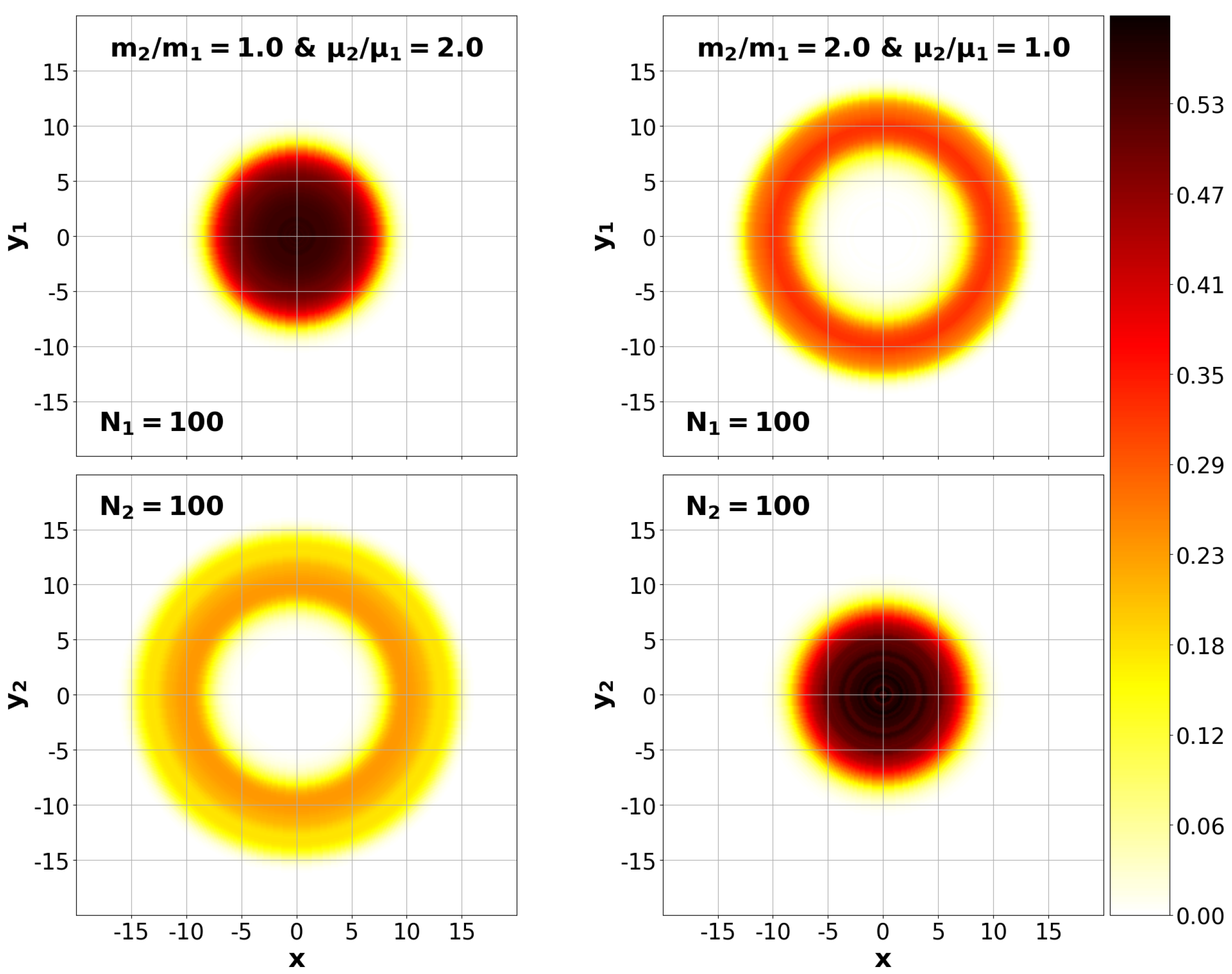
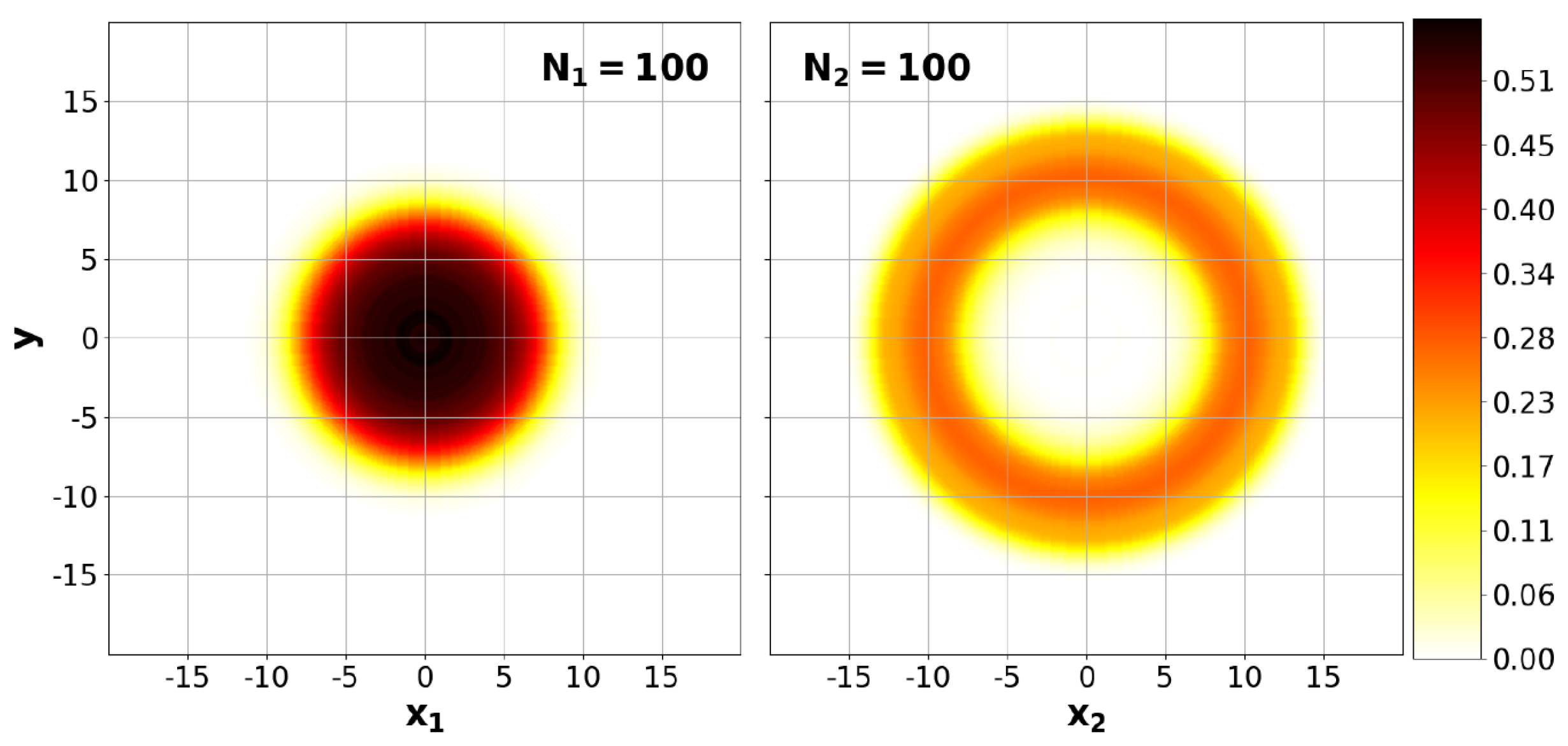
We start with the following paradigmatic mixtures: $(m_2/m_1=1,{\mu }_2/{\mu }_1=2)$ and $(m_2/m_1=2,{\mu }_2/{\mu }_1=1)$. These will allow to understand the effects of the mass and magnetic dipole moment relations between species before an exhaustive analysis of the phase diagram is performed. The pure estimators for the radial density functions $\rho \left(r\right)$ are shown in Figure 1. We observe that if the mass of the two species is the same, the particles with the larger magnetic dipole moment move out of the center and completely surround the other species. This is due to the type 2 particles repelling each other more strongly than type 1 particles do, leading the system to a configuration where type 2 particles are as separated as possible from one another and from the other species. The DMC simulation tells us that the most energetically favorable way to do this is by the second species forming a ring around the first one. Regarding the right panel in Figure 1, we see that if the magnetic dipole moment of the two species is the same, it is the lighter particles that now envelop the heavier ones. This is a direct consequence of both species being under the presence of the same confinement, as the lighter one presents a larger harmonic length.

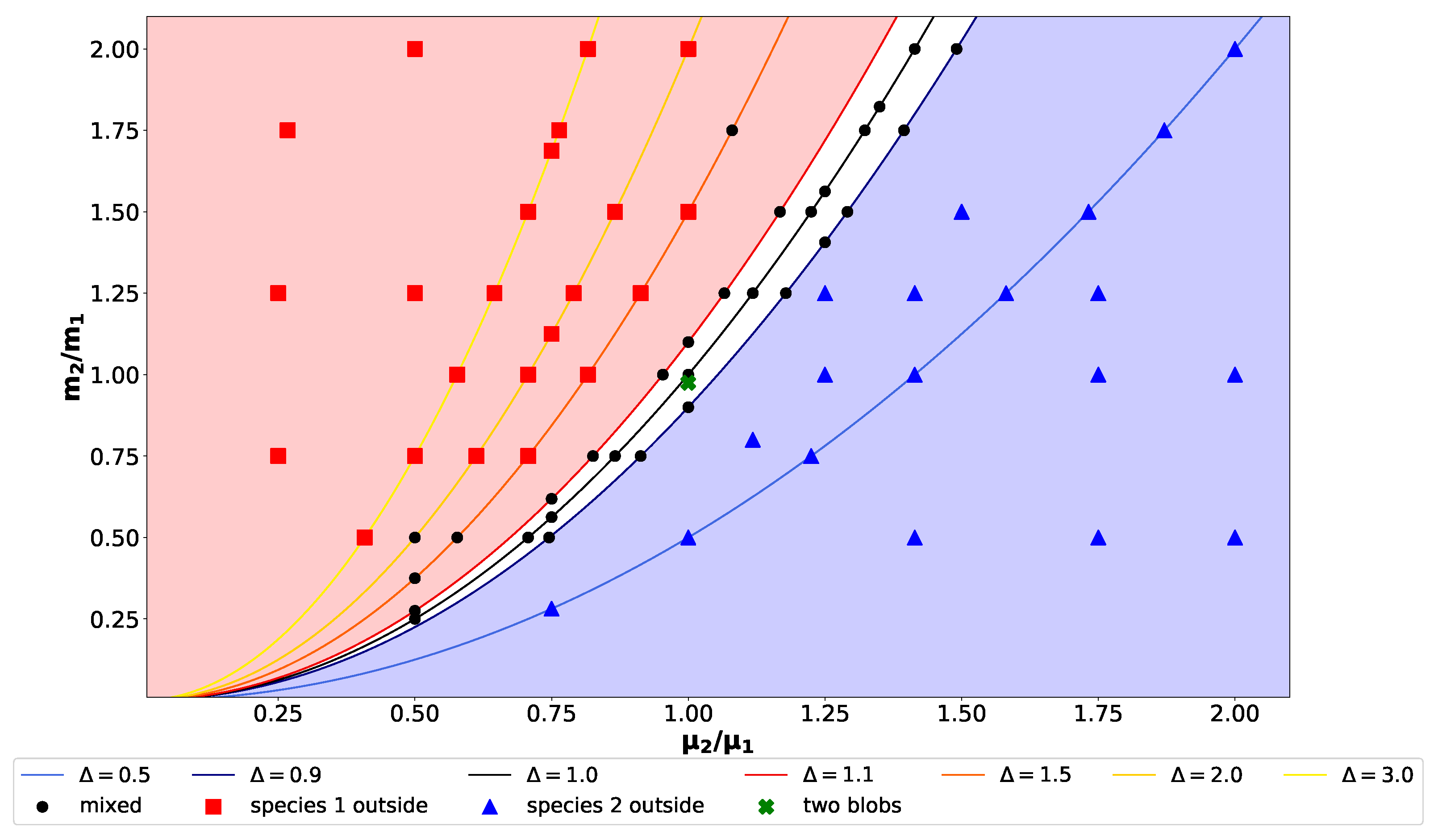
The phase diagram of the mixture is obtained by carrying out multiple simulations for different $m_2/m_1$ and ${\mu }_2/{\mu }_1$ values. From the density profiles of both species, we determine if they are miscible or not and these results are compared with the empirical criterion of Equation (32). The results are shown in Figure 2.

As it can be seen in Figure 2, the criterion (32) matches almost perfectly with the DMC results, with a very narrow region of miscibility at $0.9\lesssim \Delta \lesssim 1.1$, indicating the system’s clear tendency to phase-separate as soon as it is possible due to the repulsiveness of the DDIs. In addition, every system that phase separates does so via one species leaving the center and surrounding the other one. The farther $\Delta$ is from $1.0$, the more completely it surrounds the other, leaving the center entirely for values of $\Delta =3.0$ and $\Delta =0.5$, with complete separation already happening for values closer to $\Delta =1.0$ for specific $m_2/m_1$ and ${\mu }_2/{\mu }_1$ relations. In addition, we noticed that for the mixtures where ${\mu }_2/{\mu }_1$ is changed, the phase-separation is clearer, with one species abandoning the center entirely for values closer to $\Delta =1.0$. Moreover, let us remark how $\Delta$ can also be used to predict which particles leave the core, as for $\Delta >1.1$ species 1 does it, while for $\Delta <0.9$ it is species 2 that occupies the external shell.

There is one exception in Figure 2 corresponding to the particular values ${\mu }_2/{\mu }_1=1.0$ and $m_2/m_1=0.975$ (green point). In this case, the system does not entirely mix, but neither does it phase-separate in the usual form. As reported in Ref. [34] for 3D harmonically trapped Bose–Bose mixtures with contact interactions, in certain cases the system clearly phase-separates forming a “two-blobs” configuration, where each species occupies a semi-circumference. As the trap is isotropic, the “two-blobs” structure is degenerate and the axis, transverse to the line (2D) or surface (3D) separating the two phases, can appear in any direction. Only when one plots the structure along this transverse axis the structure can be observed. This effect produces in the density profile a maximum value which is slightly displaced with respect to the center of the trap. In our case, under an isotropic confinement the system does not phase-separate completely, and seems to only hint at such a configuration. This seems to be an exception, as we were unable to find any other case where this happened, and so we leave the analysis of this particular system to the next subsection, where we will discuss how for a given deformation of the trap, the “two-blobs” configuration can be observed before it disappears for stronger compressions.

3.2. Anisotropically Trapped Mixtures

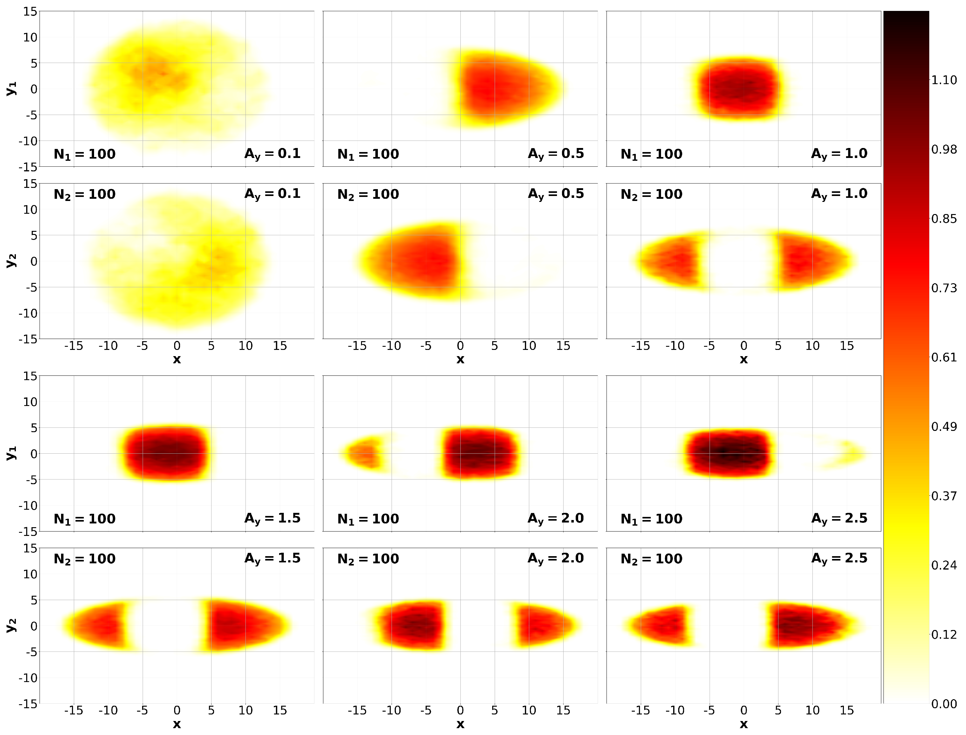
In this section, we focus on systems with $N_1=N_2=100$ particles and analyze progressively stronger sets of anisotropic harmonic confinements with $A_x=0.1$ fixed and $A_y$ changing from $0.5$ to $2.5$. We do not want $A_y$ to be too large as we do not wish to enter the one-dimensional regime; we are interested in the effects of deforming the system, not changing its behavior completely. We study three mixtures given by $(m_2/m_1=1.0, {\mu }_2/{\mu }_1=2.0)$, $(m_2/m_1=2.0, {\mu }_2/{\mu }_1=1.0)$, and $(m_2/m_1=0.975, {\mu }_2/{\mu }_1=1.0)$, which hereinafter we label as A, B, and C, respectively. Mixture A will allow us to isolate the effects of changing the magnetic dipole moment of one species and mixture B will do the same with the mass relation. Finally, mixture C, as explained in Section 3.1, seemed to hint at a two-blobs configuration under an isotropic confinement, and so we will study how it evolves as it is compressed.

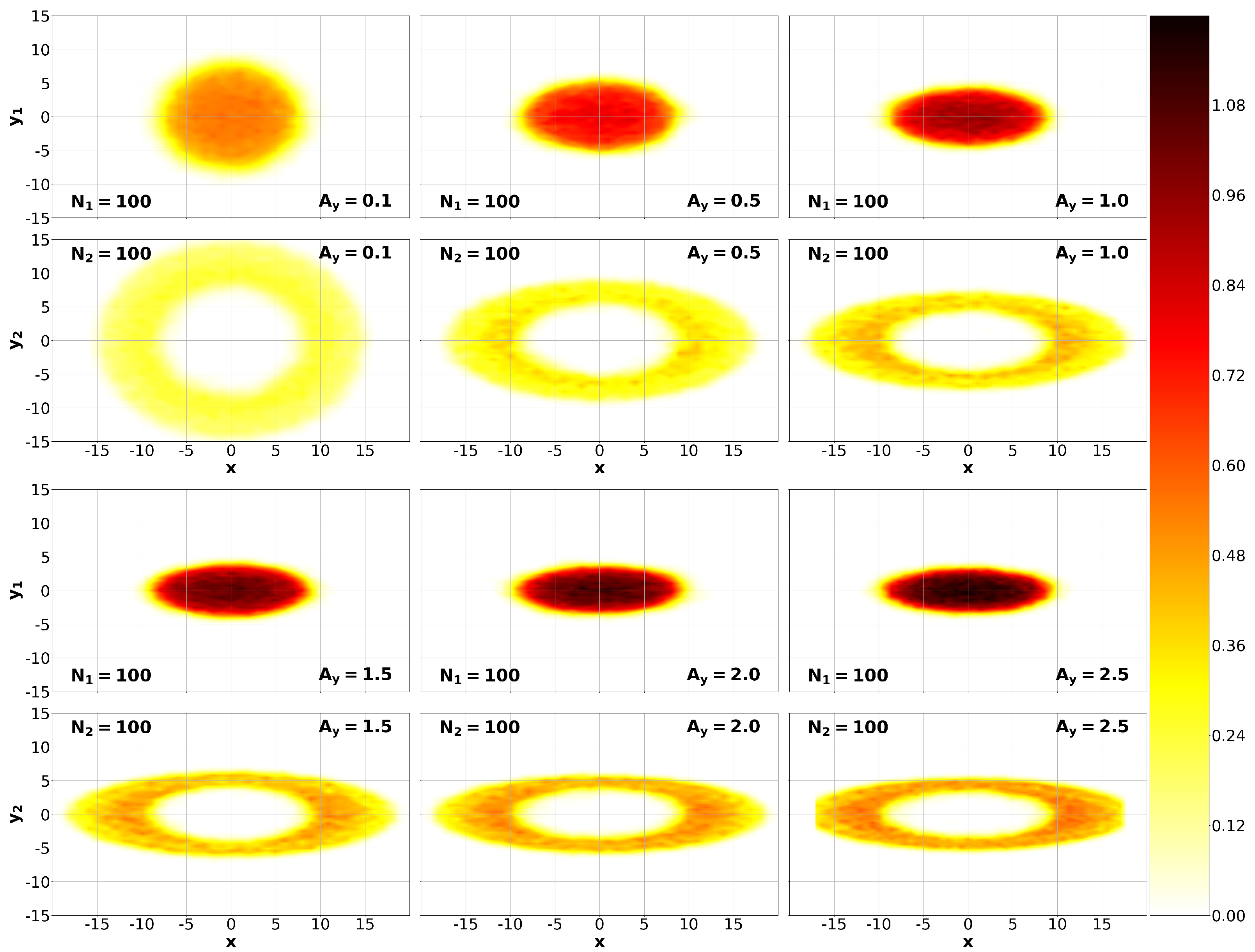
The density profiles of mixture A, obtained with pure estimators, are shown in Figure 3. In this case, the type 2 particles intra-species interactions, and the cross interactions with particles 1, are so repulsive that no matter how much we compress the system in the y-direction, particles 2 always leave the center, forming a ring surrounding the species with the smaller magnetic dipole moment. Therefore, if the DDIs are strong enough for one species compared to the other, the ring configuration is maintained throughout the compression.

The density profiles for mixture B are displayed in Figure 4. We can see that in this case the configuration is not maintained throughout the deformation. If the compression is small (see $A_y=0.5$) the ring is still present, as it is still energetically favorable for the lighter species to leave the center, surrounding the others. However, as the compression progresses, the equilibrium between the DDIs and the harmonic confinement for particles 1 cannot be reached with the ring configuration. Particles 2 now occupy the center in such a way that the second species cannot keep enough distance between themselves and the other species at small and intermediate x values for it to be energetically favorable. As a result, particles 1 form “wings” surrounding particles 2.

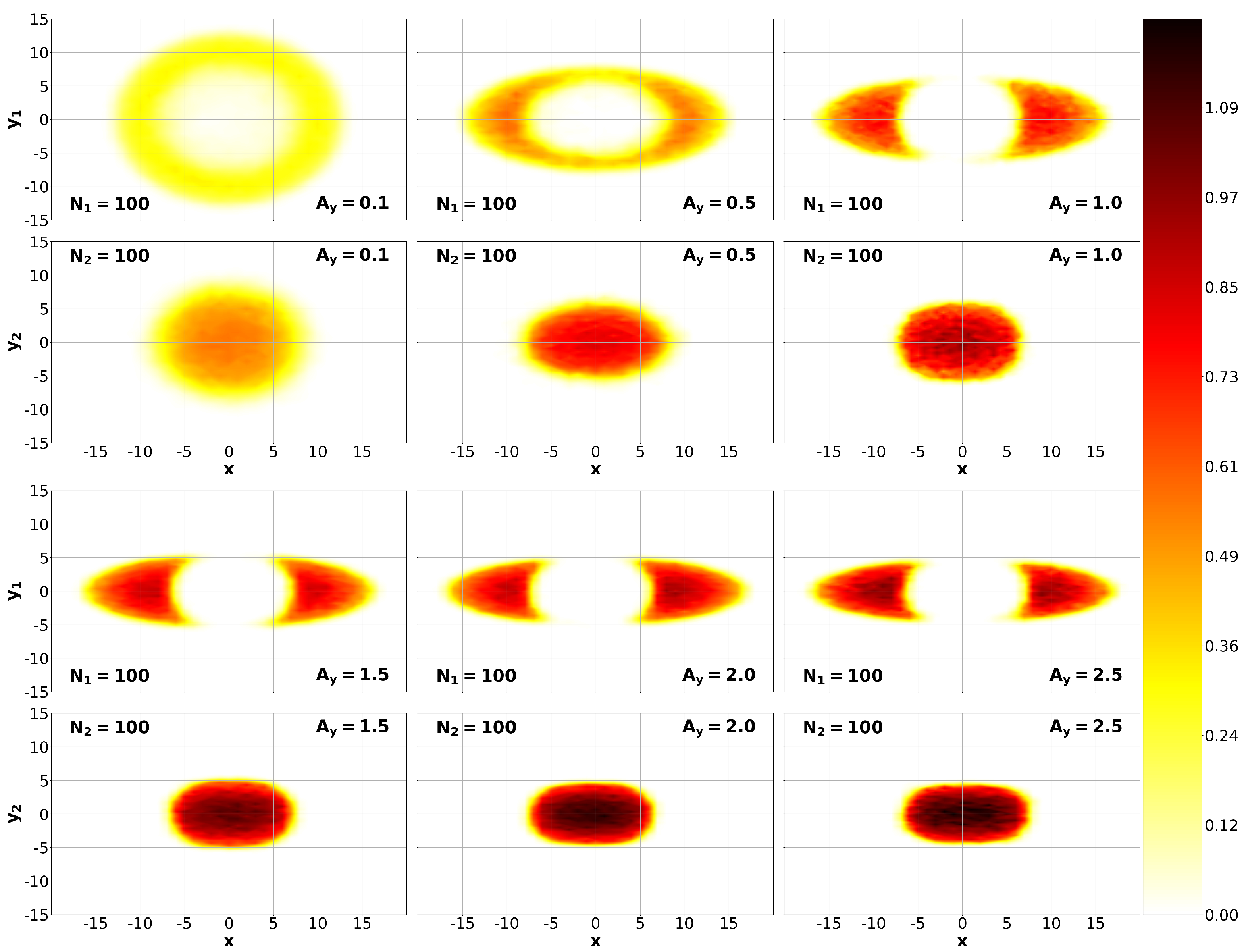
Finally, mixture C’s density profiles are shown in Figure 5. In this case, we start with the system hinting at a two-blobs configuration, which gets completely clear and defined for $A_y=0.5$. Different simulations produce two mirroring degenerate structures, with a particular species on the right or on the left (along the x-axis). In our plots, we break this degeneracy by a proper rotation. The two-blobs configuration disappears for stronger deformations, and gives way to the wing configuration described for mixture B. This system, as far as we can tell from the analyzed mixtures, is an exception, as we have been unable to find another system presenting these symmetric semi-ellipses. We suspect that this type of configuration may only appear at very particular $m_2/m_1$ and ${\mu }_2/{\mu }_1$ relations for which 1-2 interactions are the most repulsive and 1-1 and 2-2 interactions are of similar strength. In this situation, the mixture could form symmetric distributions for each species, allowing for large interparticle distances.

Any other mixed isotropic configuration that we have analyzed turns into a phase-separated system as it is compressed. As we saw in Figure 2, it required very specific mass and magnetic dipole relations between the two species for the system to be in a mixed state. Therefore, those very specific conditions move and maybe even disappear as the system is compressed and the DDIs become more repulsive. It may be possible, though, that different regions of existence for the miscible state exist for these anisotropic confinements. It is, however, beyond the scope of this work to probe the full phase-space, as it was done for the isotropic case, Figure 2.

3.3. Erbium-Dysprosium Mixture

Throughout this work we have studied a generic set of systems, given by changes in the mass and magnetic dipole moment relations between species and the deformation of the harmonic confinement applied to it. In this section, we perform a study of these effects for an Erbium-Dysprosium (Er-Dy henceforth) system, as it is the first Bose–Bose dipolar mixture that has been realized experimentally [14,15,16] and offers us a perfect opportunity to predict potentially observable configurations. Both Er and Dy are part of the magnetic rare-earth species group, and we are going to focus on the case of a ${}^{166}$Er-${}^{164}$Dy mixture, with ${}^{166}$Er having an atomic mass of $165.930293$ uma and a magnetic dipole moment of $7{\mu }_B$, and ${}^{164}$Dy having a mass of $163.929175$ and a magnetic dipole moment of $10{\mu }_B$. For convenience, we define the Er atoms as the type 1 species and the Dy ones as type 2, so that the mass and magnetic dipole moment relations characterizing the system are $m_2/m_1\simeq 0.9897$ and ${\mu }_2/{\mu }_1\simeq 1.4285$, respectively. As commented previously, we remain in a strictly 2D geometry and the interaction is the dipolar potential (2) without any short-range (contact) repulsive interaction. In this 2D limit, and all the dipoles oriented perpendicularly to the plane, the dipolar interaction is fully repulsive and the contact interaction would not change the present results in a significant way. Instead, in 3D the contact interaction is crucial to avoid the collapse that the dipolar potential produces [10].

We start with a balanced mixture of Er-Dy atoms, with $N_1=N_2=100$ particles each, under the presence of an isotropic harmonic confinement of strength $A=0.1$. The pure density profiles for this case are shown in Figure 6. As it can be clearly seen, under these conditions the system phase-separates, with the Dy atoms leaving the center and surrounding the Er particles. In this case $m_2/m_1\approx 1$, meaning the mass difference between species, is not a key factor, and the inmiscibility is due to the Dy atoms having a significantly larger magnetic dipole moment, which forces them out of the center due to the stronger repulsive DDI interactions between themselves and the Er atoms.

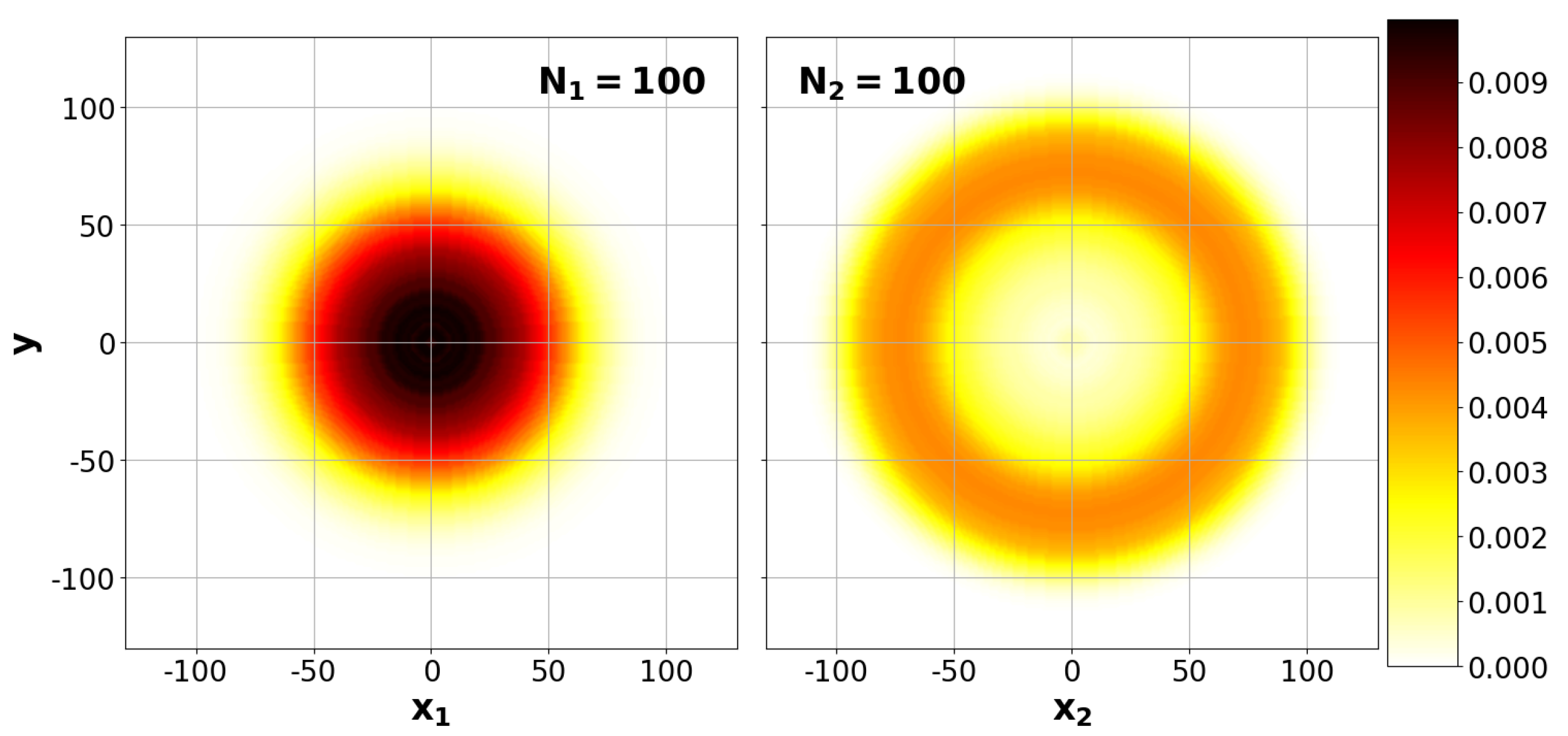
In Figure 6, the confinement produces a central density of 1 in dipolar units. This density is larger than the typical densities in experiments with dipolar gases. To analyze the influence of the density and approach the experimental conditions better, we have simulated the mixture with a smaller confinement. By choosing $A=1·{10}^{-5}$ we observe central densities of $0.01$ that are in the range of confined dipolar gases in experiments [48]. The results obtained are shown in Figure 7. As one can see, the reduction of the density does not affect the prediction regarding the phase separated configuration of the 2D Er-Dy mixtures.

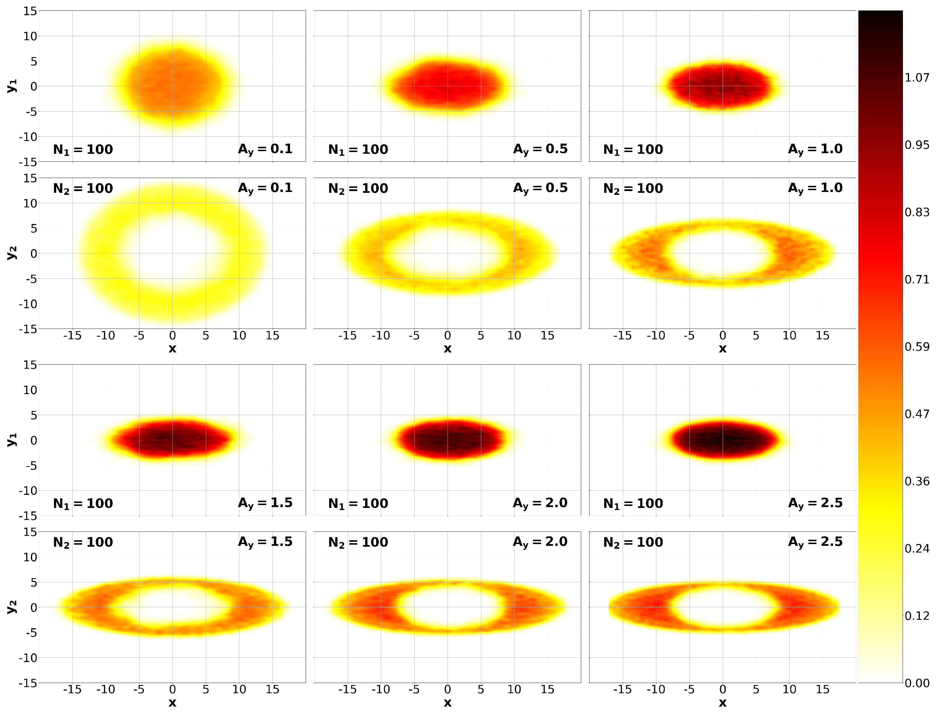
We expose the mixture to progressively stronger potentials in the y-direction, in the same way as in Section 3.1. The pure density profiles are shown in Figure 8. In this case, due to the mass relation between species essentially not playing any role, it is the DDIs that are integral to the obtained spatial configurations. These are so repulsive that, again, the ring configuration is the most favorable one, regardless of the applied deformation in the y-direction. However, as we can see from the $A_y=2.5$ result, it seems that by pushing the system further, the wing configuration could eventually appear.

4. Discussion

In this study, we have presented a thorough analysis of dipolar binary Bose–Bose mixtures at zero temperature in two dimensions, confined harmonically in the $xy$ plane. The results have been obtained by a combination of two quantum Monte Carlo methods: variational Monte Carlo, for the optimization of the trial wave function, and diffusion Monte Carlo, to get a statistically exact solution by means of solving the Schrödinger equation in imaginary time. With this, we have been able to map the miscibility of balanced mixtures under an isotropic harmonic confinement, studied anisotropic confinements by progressively applying a stronger trapping in the y direction, and performed a study of the Erbium-Dysprosium mixture, the first dipolar Bose–Bose mixture realized experimentally.

In Section 3.1, we performed a complete analysis of mixtures with a total number of particles of $N=200$ under an isotropic harmonic confinement of strength $A=0.1$. We saw how the masses were equal, as the species with the larger magnetic dipole moment left the center and surrounded the other ones in a ring configuration, while ${\mu }_1={\mu }_2$ led to the lighter particles leaving the core as a consequence of having a larger harmonic characteristic length. We studied the miscibility of the system as a function of $m_2/m_1$ and ${\mu }_2/{\mu }_1$ with the help of a dimensionless parameter $\Delta$ (see Equation (32) and Figure 2), and concluded that the miscibility region of the system is very narrow, as it only occurs around $0.9\lesssim \Delta \lesssim 1.1$, otherwise the system phase-separates in two different ways: for $\Delta >1$ species 1 leaves the center, while for $\Delta <1$ it is species 2 that abandons the core. Every system studied that phase-separated did so by means of this ’ring’ configuration in which one species occupies the core, and the other encircles it, as due to the repulsive DDIs this allows for the maximum distance between particles of both the same and different species.

In Section 3.2, we focused on analyzing three mixtures (A, B, and C) given under progressively stronger confinements in the y direction, keeping the x component constant. We concluded that by changing the dipole moments, the ring configuration remained the stable one in the deformation regime studied. When the mass ratio is changed, under strong enough compression, the ring configuration turns to a wing structure, in which the lighter species is pushed to the edges of the system in the x axis. In addition, we studied a very particular case, an exception from Section 3.1, the $(m_2/m_1=0.975, {\mu }_2/{\mu }_1=1)$ mixture, which under an isotropic confinement hinted at a ’two-blobs’ configuration, in which two symmetrical semi-circumferences are formed by each species separately [34] for a simpler contact interaction in a three-dimensional case. This system, under a moderately strong deformation, turns to a two-blobs configuration along the squeezed axis, which transformed into the wing one under stronger compressions. We tried to find other systems with this behavior, but we were ultimately unable to discover them.

To conclude, we studied the Er-Dy mixture, the first experimentally realized one [14,15,16], in order to make predictions on its miscibility. We observe how under an isotropic confinement the mixture phase-separated, with the Dy atoms leaving the center due to their greater magnetic dipole moments. We then analyzed the same mixture under progressively stronger confinements in the y direction and observed how the ring configuration held for every single strength that we applied. The total number of particles in the DMC simulations is clearly smaller than the corresponding one in experiments because of computer limitations. Nevertheless, we are confident that the parameter $\Delta$ defined in our work would also be applicable in mixtures with a realistic number of particles since adimensional $\Delta$ contains the relevant factors entering into the problem. Recent experiments on Er-Dy mixtures in three dimensions show that the system prefers to be phase separated due to an overall repulsion between the two species. Moreover, the gravitational sag between both species, due to their different masses, makes it difficult to get a full overlap between both species [16]. It would be interesting to deform the trapping potential and approach the 2D limit, with the magnetic moments perpendicular to the plane, because then the gravitational effect would be reduced and thus the possible miscibility between both components could be better resolved. We also hope that our work can stimulate the analysis of the dipolar mixture in two dimensions within mean-field theory, which can be compared with our DMC results. A similar study, using the Gross–Pitaevskii equation, was recently carried out for three-dimensional dipolar mixtures [49].

References

- Pethick, C.J.; Smith, H. Bose–Einstein Condensation in Dilute Gases, 2nd ed.; Cambridge University Press: Cambridge, UK, 2008. [Google Scholar]
- Georgescu, I.M.; Ashhab, S.; Nori, F. Quantum simulation. Rev. Mod. Phys. 2014, 86, 153–185. [Google Scholar] [CrossRef] [Green Version]
- Altman, E.; Brown, K.R.; Carleo, G.; Carr, L.D.; Demler, E.; Chin, C.; DeMarco, B.; Economou, S.E.; Eriksson, M.A.; Fu, K.M.C.; et al. Quantum Simulators: Architectures and Opportunities. PRX Quantum 2021, 2, 017003. [Google Scholar] [CrossRef]
- Lahaye, T.; Menotti, C.; Santos, L.; Lewenstein, M.; Pfau, T. The physics of dipolar bosonic quantum gases. Rep. Prog. Phys. 2009, 72, 126401. [Google Scholar] [CrossRef]
- Koch, T.; Lahaye, T.; Metz, J.; Fröhlich, B.; Griesmaier, A.; Pfau, T. Stabilization of a purely dipolar quantum gas against collapse. Nat. Phys. 2008, 4, 218–222. [Google Scholar] [CrossRef] [Green Version]
- Lu, M.; Burdick, N.Q.; Youn, S.H.; Lev, B.L. Strongly Dipolar Bose-Einstein Condensate of Dysprosium. Phys. Rev. Lett. 2011, 107, 190401. [Google Scholar] [CrossRef] [PubMed]
- Aikawa, K.; Frisch, A.; Mark, M.; Baier, S.; Rietzler, A.; Grimm, R.; Ferlaino, F. Bose-Einstein condensation of erbium. Phys. Rev. Lett. 2012, 108, 210401. [Google Scholar] [CrossRef] [Green Version]
- Norcia, M.A.; Ferlaino, F. New opportunites for interactions and control with ultracold lanthanides. arXiv 2021, arXiv:2108.04491. [Google Scholar]
- Ferrier-Barbut, I.; Kadau, H.; Schmitt, M.; Wenzel, M.; Pfau, T. Observation of Quantum Droplets in a Strongly Dipolar Bose Gas. Phys. Rev. Lett. 2016, 116, 215301. [Google Scholar] [CrossRef]
- Böttcher, F.; Wenzel, M.; Schmidt, J.N.; Guo, M.; Langen, T.; Ferrier-Barbut, I.; Pfau, T.; Bombín, R.; Sánchez-Baena, J.; Boronat, J.; et al. Dilute dipolar quantum droplets beyond the extended Gross-Pitaevskii equation. Phys. Rev. Res. 2019, 1, 033088. [Google Scholar] [CrossRef] [Green Version]
- Tanzi, L.; Lucioni, E.; Famà, F.; Catani, J.; Fioretti, A.; Gabbanini, C.; Bisset, R.N.; Santos, L.; Modugno, G. Observation of a Dipolar Quantum Gas with Metastable Supersolid Properties. Phys. Rev. Lett. 2019, 122, 130405. [Google Scholar] [CrossRef] [Green Version]
- Böttcher, F.; Schmidt, J.N.; Wenzel, M.; Hertkorn, J.; Guo, M.; Langen, T.; Pfau, T. Transient Supersolid Properties in an Array of Dipolar Quantum Droplets. Phys. Rev. X 2019, 9, 011051. [Google Scholar] [CrossRef] [Green Version]
- Chomaz, L.; Petter, D.; Ilzhöfer, P.; Natale, G.; Trautmann, A.; Politi, C.; Durastante, G.; van Bijnen, R.M.W.; Patscheider, A.; Sohmen, M.; et al. Long-Lived and Transient Supersolid Behaviors in Dipolar Quantum Gases. Phys. Rev. X 2019, 9, 021012. [Google Scholar] [CrossRef] [Green Version]
- Ravensbergen, C.; Corre, V.; Soave, E.; Kreyer, M.; Kirilov, E.; Grimm, R. Production of a degenerate Fermi-Fermi mixture of dysprosium and potassium atoms. Phys. Rev. A 2018, 98, 063624. [Google Scholar] [CrossRef] [Green Version]
- Trautmann, A.; Ilzhöfer, P.; Durastante, G.; Politi, C.; Sohmen, M.; Mark, M.J.; Ferlaino, F. Dipolar Quantum Mixtures of Erbium and Dysprosium Atoms. Phys. Rev. Lett. 2018, 121, 213601. [Google Scholar] [CrossRef] [PubMed] [Green Version]
- Politi, C.; Trautmann, A.; Ilzhöfer, P.; Durastante, G.; Mark, M.J.; Modugno, M.; Ferlaino, F. Study of the inter-species interactions in an ultracold dipolar mixture. arXiv 2021, arXiv:2110.09980. [Google Scholar]
- Wilson, R.M.; Ticknor, C.; Bohn, J.L.; Timmermans, E. Roton immiscibility in a two-component dipolar Bose gas. Phys. Rev. A 2012, 86, 033606. [Google Scholar] [CrossRef] [Green Version]
- Kumar, R.K.; Muruganandam, P.; Tomio, L.; Gammal, A. Miscibility in coupled dipolar and non-dipolar Bose–Einstein condensates. J. Phys. Commun. 2017, 1, 035012. [Google Scholar] [CrossRef]
- Xi, K.T.; Byrnes, T.; Saito, H. Fingering instabilities and pattern formation in a two-component dipolar Bose-Einstein condensate. Phys. Rev. A 2018, 97, 023625. [Google Scholar] [CrossRef] [Green Version]
- Kumar, R.K.; Tomio, L.; Gammal, A. Spatial separation of rotating binary Bose-Einstein condensates by tuning the dipolar interactions. Phys. Rev. A 2019, 99, 043606. [Google Scholar] [CrossRef] [Green Version]
- Kumar, R.K.; Tomio, L.; Malomed, B.A.; Gammal, A. Vortex lattices in binary Bose-Einstein condensates with dipole-dipole interactions. Phys. Rev. A 2017, 96, 063624. [Google Scholar] [CrossRef] [Green Version]
- Bisset, R.N.; Ardila, L.A.P.n.; Santos, L. Quantum Droplets of Dipolar Mixtures. Phys. Rev. Lett. 2021, 126, 025301. [Google Scholar] [CrossRef] [PubMed]
- Smith, J.C.; Baillie, D.; Blakie, P.B. Quantum Droplet States of a Binary Magnetic Gas. Phys. Rev. Lett. 2021, 126, 025302. [Google Scholar] [CrossRef] [PubMed]
- Myatt, C.J.; Burt, E.A.; Ghrist, R.W.; Cornell, E.A.; Wieman, C.E. Production of Two Overlapping Bose-Einstein Condensates by Sympathetic Cooling. Phys. Rev. Lett. 1997, 78, 586–589. [Google Scholar] [CrossRef]
- Hall, D.S.; Matthews, M.R.; Ensher, J.R.; Wieman, C.E.; Cornell, E.A. Dynamics of Component Separation in a Binary Mixture of Bose-Einstein Condensates. Phys. Rev. Lett. 1998, 81, 1539–1542. [Google Scholar] [CrossRef] [Green Version]
- Maddaloni, P.; Modugno, M.; Fort, C.; Minardi, F.; Inguscio, M. Collective Oscillations of Two Colliding Bose-Einstein Condensates. Phys. Rev. Lett. 2000, 85, 2413–2417. [Google Scholar] [CrossRef] [Green Version]
- Papp, S.B.; Pino, J.M.; Wieman, C.E. Tunable Miscibility in a Dual-Species Bose-Einstein Condensate. Phys. Rev. Lett. 2008, 101, 040402. [Google Scholar] [CrossRef] [Green Version]
- Modugno, G.; Modugno, M.; Riboli, F.; Roati, G.; Inguscio, M. Two Atomic Species Superfluid. Phys. Rev. Lett. 2002, 89, 190404. [Google Scholar] [CrossRef] [Green Version]
- McCarron, D.J.; Cho, H.W.; Jenkin, D.L.; Köppinger, M.P.; Cornish, S.L. Dual-species Bose-Einstein condensate of 87Rb and 133Cs. Phys. Rev. A 2011, 84, 011603. [Google Scholar] [CrossRef] [Green Version]
- Pasquiou, B.; Bayerle, A.; Tzanova, S.M.; Stellmer, S.; Szczepkowski, J.; Parigger, M.; Grimm, R.; Schreck, F. Quantum degenerate mixtures of strontium and rubidium atoms. Phys. Rev. A 2013, 88, 023601. [Google Scholar] [CrossRef] [Green Version]
- Wacker, L.; Jørgensen, N.B.; Birkmose, D.; Horchani, R.; Ertmer, W.; Klempt, C.; Winter, N.; Sherson, J.; Arlt, J.J. Tunable dual-species Bose-Einstein condensates of 39K and 87Rb. Phys. Rev. A 2015, 92, 053602. [Google Scholar] [CrossRef] [Green Version]
- Chen, L.; Zhu, C.; Zhang, Y.; Pu, H. Spin-exchange-induced spin-orbit coupling in a superfluid mixture. Phys. Rev. A 2018, 97, 031601. [Google Scholar] [CrossRef] [Green Version]
- Lee, K.L.; Jørgensen, N.B.; Liu, I.K.; Wacker, L.; Arlt, J.J.; Proukakis, N.P. Phase separation and dynamics of two-component Bose-Einstein condensates. Phys. Rev. A 2016, 94, 013602. [Google Scholar] [CrossRef] [Green Version]
- Cikojević, V.; Markić, L.V.; Boronat, J. Harmonically trapped Bose–Bose mixtures: A quantum Monte Carlo study. New J. Phys. 2018, 20, 085002. [Google Scholar] [CrossRef]
- Astrakharchik, G.E.; Boronat, J.; Kurbakov, I.L.; Lozovik, Y.E. Quantum Phase Transition in a Two-Dimensional System of Dipoles. Phys. Rev. Lett. 2007, 98, 060405. [Google Scholar] [CrossRef] [PubMed] [Green Version]
- Bombin, R.; Boronat, J.; Mazzanti, F. Dipolar Bose Supersolid Stripes. Phys. Rev. Lett. 2017, 119, 250402. [Google Scholar] [CrossRef] [Green Version]
- Bombín, R.; Mazzanti, F.; Boronat, J. Berezinskii-Kosterlitz-Thouless transition in two-dimensional dipolar stripes. Phys. Rev. A 2019, 100, 063614. [Google Scholar] [CrossRef] [Green Version]
- Pawłowski, K.; Bienias, P.; Pfau, T.; Rzążewski, K. Correlations of a quasi-two-dimensional dipolar ultracold gas at finite temperatures. Phys. Rev. A 2013, 87, 043620. [Google Scholar] [CrossRef] [Green Version]
- Guardiola, R. Monte carlo methods in quantum many-body theories. In Microscopic Quantum Many-Body Theories and Their Applications; Springer: Berlin/Heidelberg, Germany, 2007; pp. 269–336. [Google Scholar] [CrossRef]
- Vrbik, J.; Rothstein, S.M. Quadratic accuracy diffusion Monte Carlo. J. Comput. Phys. 1986, 63, 130–139. [Google Scholar] [CrossRef]
- Boronat, J.; Casulleras, J. Monte Carlo analysis of an interatomic potential for He. Phys. Rev. B 1994, 49, 8920–8930. [Google Scholar] [CrossRef] [Green Version]
- Boronat, J. Monte Carlo simulations at zero temperature: Helium in one, two and three dimensions. In Microscopic Approaches to Quantum Liquids in Confined Geometries; Krotscheck, E., Navarro, J., Eds.; World Scientific: Singapore, 2002; p. 21. [Google Scholar]
- Casulleras, J.; Boronat, J. Unbiased estimators in quantum Monte Carlo methods: Application to liquid 4He. Phys. Rev. B 1995, 52, 3654. [Google Scholar] [CrossRef] [Green Version]
- Jastrow, R. Many-Body Problem with Strong Forces. Phys. Rev. 1955, 98, 1479–1484. [Google Scholar] [CrossRef]
- Macia, A. Microscopic Description of Two Dimensional Dipolar Quantum Gases. Ph.D. Thesis, Universitat Politecnica de Catalunya, Barcelona, Spain, 2015. [Google Scholar] [CrossRef]
- Kim, S.H.; Won, C.; Oh, S.D.; Jhe, W. Two-dimensional Gross-Pitaevskii Equation: Theory of Bose-Einstein Condensation and the Vortex State. arXiv 1999, arXiv:cond-mat/9904087. [Google Scholar]
- Karle, V.; Defenu, N.; Enss, T. Coupled superfluidity of binary Bose mixtures in two dimensions. Phys. Rev. A 2019, 99, 063627. [Google Scholar] [CrossRef] [Green Version]
- Hertkorn, J.; Schmidt, J.N.; Böttcher, F.; Guo, M.; Schmidt, M.; Ng, K.S.H.; Graham, S.D.; Büchler, H.P.; Langen, T.; Zwierlein, M.; et al. Density Fluctuations across the Superfluid-Supersolid Phase Transition in a Dipolar Quantum Gas. Phys. Rev. X 2021, 11, 011037. [Google Scholar] [CrossRef]
- Lee, A.C.; Baillie, D.; Blakie, P.B.; Bisset, R.N. Miscibility and stability of dipolar bosonic mixtures. Phys. Rev. A 2021, 103, 063301. [Google Scholar] [CrossRef]
Figure 1.
Left column: pure estimators of the density for . Right column: pure estimator of the density for .
Figure 2.
Miscibility of balanced mixtures as a function of and for and . The points indicate the performed simulations.
Figure 3.
Mixture A. First and second rows, from left to right: pure density profiles for , and , respectively. Third and fourth rows, from left to right: density profiles for , and , respectively. In all cases .
Figure 4.
Mixture B. First and second rows, from left to right: pure density profiles for , and , respectively. Third and fourth rows, from left to right: density profiles for , and , respectively. In all cases .
Figure 5.
Mixture C. First and second rows, from left to right: pure density profiles for , and , respectively. Third and fourth rows, from left to right: density profiles for , and , respectively. In all cases .
Figure 6.
for an Er-Dy balanced mixture under an isotropic confinement of value in reduced dipolar units.
Figure 7.
Figure 8.
First and second rows, from left to right: pure density profiles of the Er-Dy mixture for , and , respectively. Third and fourth row, from left to right: density profiles for , and , respectively. In all cases .
Publisher’s Note: MDPI stays neutral with regard to jurisdictional claims in published maps and institutional affiliations. |
© 2022 by the authors. Licensee MDPI, Basel, Switzerland. This article is an open access article distributed under the terms and conditions of the Creative Commons Attribution (CC BY) license (https://creativecommons.org/licenses/by/4.0/).
Share and Cite
MDPI and ACS Style
Pradas, S.; Boronat, J. Mixtures of Dipolar Gases in Two Dimensions: A Quantum Monte Carlo Study. Condens. Matter 2022, 7, 32. https://0-doi-org.brum.beds.ac.uk/10.3390/condmat7020032
AMA Style
Pradas S, Boronat J. Mixtures of Dipolar Gases in Two Dimensions: A Quantum Monte Carlo Study. Condensed Matter. 2022; 7(2):32. https://0-doi-org.brum.beds.ac.uk/10.3390/condmat7020032
Chicago/Turabian StylePradas, Sergi, and Jordi Boronat. 2022. "Mixtures of Dipolar Gases in Two Dimensions: A Quantum Monte Carlo Study" Condensed Matter 7, no. 2: 32. https://0-doi-org.brum.beds.ac.uk/10.3390/condmat7020032