Article

Real-Time Accelerator Diagnostic Tools for the MAX IV Storage Rings

MAX IV Laboratory, Lund University, Fotongatan 2, 224 84 Lund, Sweden
*
Author to whom correspondence should be addressed.
Submission received: 22 July 2020 / Revised: 29 August 2020 / Accepted: 31 August 2020 / Published: 3 September 2020

Abstract

:
In this paper, beam diagnostic and monitoring tools developed by the MAX IV Operations Group are discussed. In particular, beam position monitoring and accelerator tunes visualization software tools, as well as tools that directly influence the beam quality and stability, are introduced. An availability and downtime monitoring application is also presented.

1. Introduction

The MAX IV laboratory [1] is a synchrotron radiation facility in Lund, Sweden. MAX IV is the first Multi-Bend Achromat (MBA) Synchrotron Light Source in the world and provides scientists with the most brilliant X-rays for research. The laboratory was inaugurated in June 2016 and consists of two storage rings operated at 1.5 and 3 GeV providing spontaneous radiation of high brilliance over a broad spectral range. The 1.5 GeV ring has a circumference of 96 m and employs a double-bend achromat lattice to produce an emittance of 6 nm rad. The 3 GeV storage ring on the other hand is aimed towards ultralow emittance to generate high brilliance hard X-rays. The design of the 3 GeV storage ring includes many novel technologies, such as MBA lattice, and a compact, fully-integrated magnet design. This results in a circumference of 528 m and an emittance as low as 0.2 nm rad [2]. A linear accelerator (linac) works as a full-energy injector for the storage rings, as well as a driver to a Short Pulse Facility (SPF). The prime sources for synchrotron radiation at the rings are optimized insertion devices (IDs), providing intense X-ray light for each of the MAX IV beamlines. Figure 1 shows a floor map the MAX IV laboratory, showing the location of the beamlines and of the storage rings. The linac is the straight section at the left of the figure.
This article is organized as follows. Section 2 briefly summarizes the nominal operation conditions of the storage rings and of the SPF. In Section 3, a new software tool which displays the beam position’s evolution over time and the accelerator tunes’ evolution over time using two-dimensional colormap spectrograms is presented. A tool that reduces the impact of changing orbit bumps for the MAX IV beamlines is presented in Section 4. Section 5 introduces an application for adjusting the master oscillator’s radio-frequency of a storage ring that is nearly transparent for beamlines. Section 6 describes the MAX IV downtime web-application used for registering and monitoring the availability and downtime of the MAX IV accelerators with automatized plotting capabilities allowing for prompt statistical analysis of events. Section 7 presents a brief discussion of the results. Conclusions are outlined in Section 8.

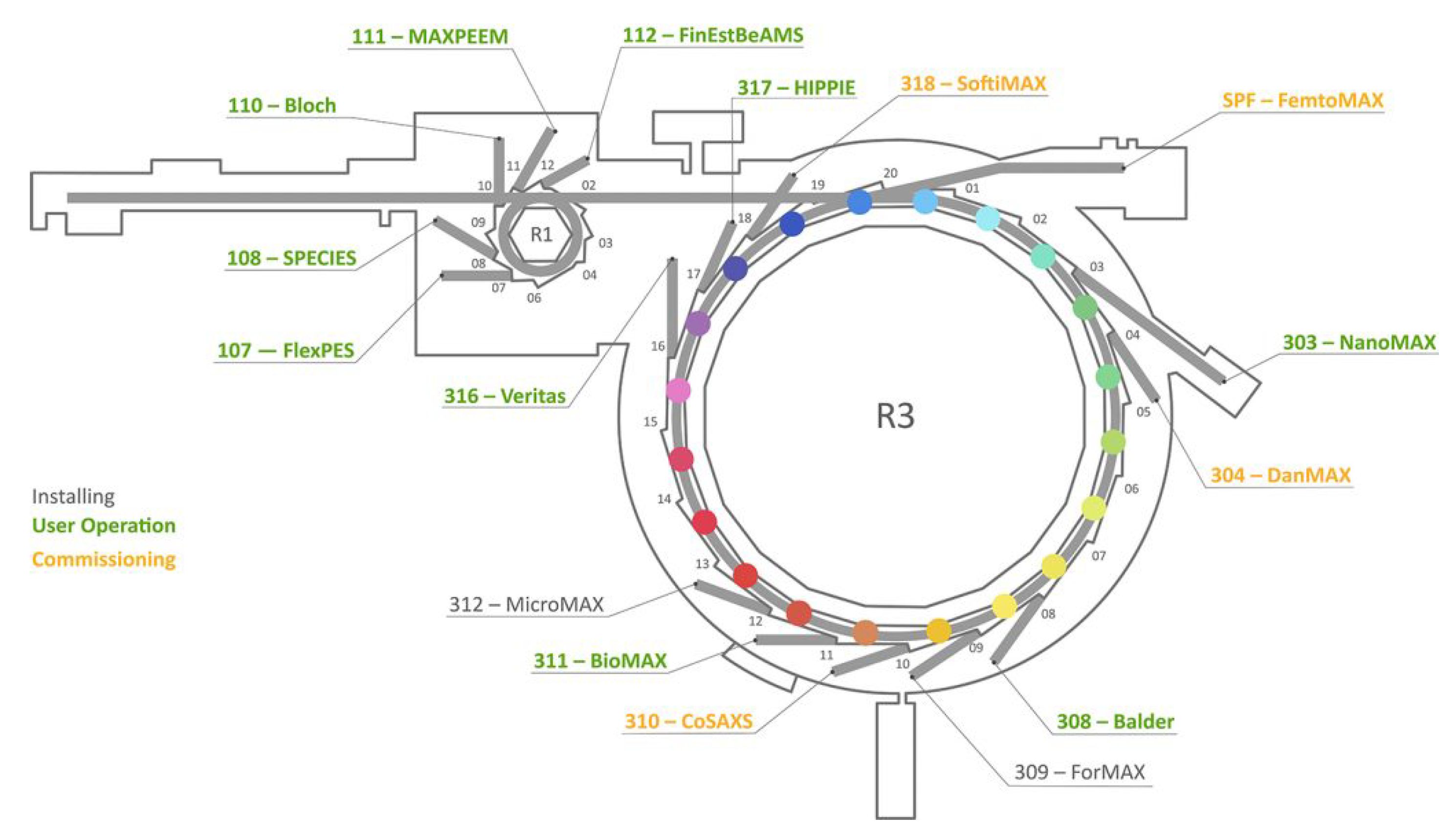
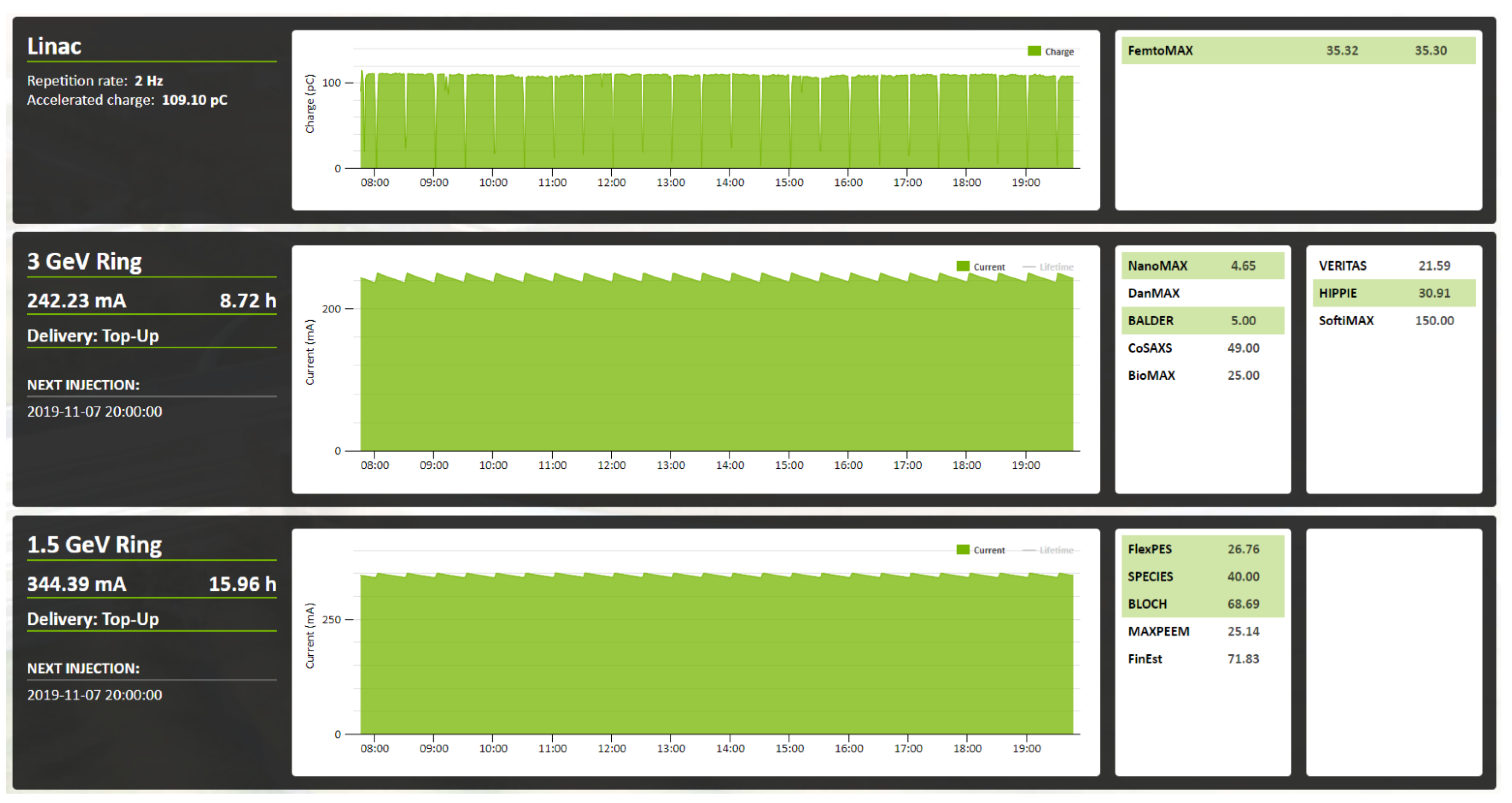
2. MAX IV Accelerator Operations

The MAX IV storage rings [3] currently operate in a 30-min and 10-min top-up injection mode for the 1.5 and 3 GeV during user delivery, respectively. High bunch charge is delivered to the SPF in-between injections. Different injection methods are used to fill each storage ring. In the 1.5 GeV storage ring, injections are accomplished using a single dipole kicker magnet, which although efficient is not transparent (beam size increase larger than 10%) to users, leading to betatron oscillations of the stored beam with amplitudes of the order of several millimeters. In the 3 GeV storage ring, a Multipole Injection Kicker (MIK) method is used, which delivers quasi-transparent injections (beam size growth of ≈6 % during the first 5 turns after the firing of the MIK) [4]. Under nominal conditions, the 3 GeV storage ring operates with 166 filled radio frequency (RF) buckets, out of a maximum (harmonic number) of 176, while the 1.5 GeV ring operates at 32 even-filled RF buckets.
Both storage rings employ passive harmonic (Landau) RF cavities [5]. The main function of the harmonic cavities is to generate a voltage which counteracts the longitudinal focusing at the bunch center of the main RF voltage, lengthening the bunch, and decreasing the charge density, thus damping instabilities and increasing the Touschek-dominated lifetime.
The 3 GeV and 1.5 GeV rings make use of a number of feedback systems to deliver stable and reliable beams. These include main cavity field amplitude and phase, main cavity frequency, and Landau cavity field amplitude, all implemented in an FPGA-based low level RF-system [6]. The 3 GeV ring uses also feedback to damp Robinson mode oscillations [7]. A digital Bunch-By-Bunch (BBB) feedback is used to damp coupled bunch modes and as a diagnostic tool [8,9].
A slow orbit feedback (SOFB) [10] loop is used in both storage rings to handle drifts. The main goal of this is to keep the electron orbit as constant as possible at all times. Using information from the beam position monitors (BPMs), which measure the transverse position of the beam along the storage ring, dipole corrector magnets currents are adjusted so that the beam orbit is corrected towards offsets or a pre-defined golden orbit [11]. The SOFB loop updates at a 10 Hz rate.
A feedback system that acts directly on the accelerator radio frequency master oscillator (MO RF) is used in order to keep the energy contribution from the storage ring’s corrector magnets constant. In the 1.5 GeV ring, a tune feedback is used in order to keep the betatron tunes close to a predefined optimal value. While the tune feedback system itself makes use of the ring’s quadrupole magnets and pole-face strips that are installed in dipole magnets as actuators, the betatron tunes are themselves obtained by the ring’s BBB system. The main feedback systems used at the MAX IV storage rings are shown in Table 1.
For completeness, a summary of key delivery parameters for the 1.5 and 3 GeV storage rings are presented in Table 2 and Table 3, respectively.
The current nominal operation conditions for the SPF [12] aim at delivering 100 pC charge per bunch at a repetition rate of 2 Hz. To achieve this, electrons are extracted from a copper photo-cathode using a laser pulse, then accelerated to 3 GeV. The bunches are compressed in two stages, at 233 MeV and at the full 3 GeV, to about 100 fs. Then the beam goes through the two undulators of the SPF, generating equally short x-ray pulses. As in the rings, there is a feedback on the trajectory, keeping the beam at the center of the quadrupole magnets.
Figure 2 shows the facility status in November 2019. The status page shows the current stored in the two storage rings, the charge delivered to the SPF at present time and the evolution of the stored current during the previous 12 h. It also shows the positions of the undulator gaps and the status of the beam shutters at all beamlines. A closed gap means that synchrotron light is produced by a beamline’s insertion device whilst open shutters, indicated by highlighting the beamline name in green, means that the beamline is open to take the light produced by its insertion device. As can be seen from the plot, the linac performed excellently as injector providing beam current top-up every 30 min, as well as high bunch charge (100 pC) to the SPF.

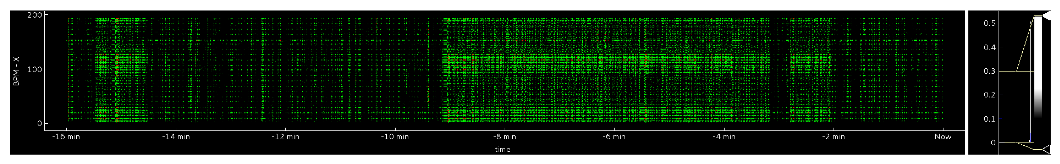
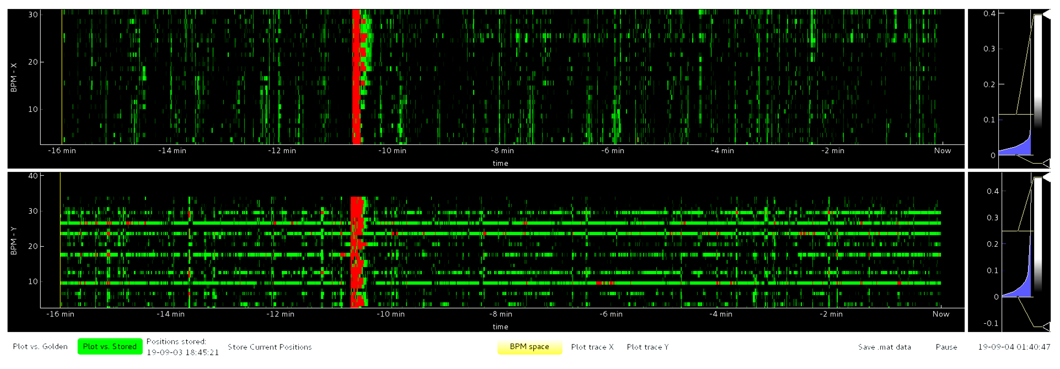
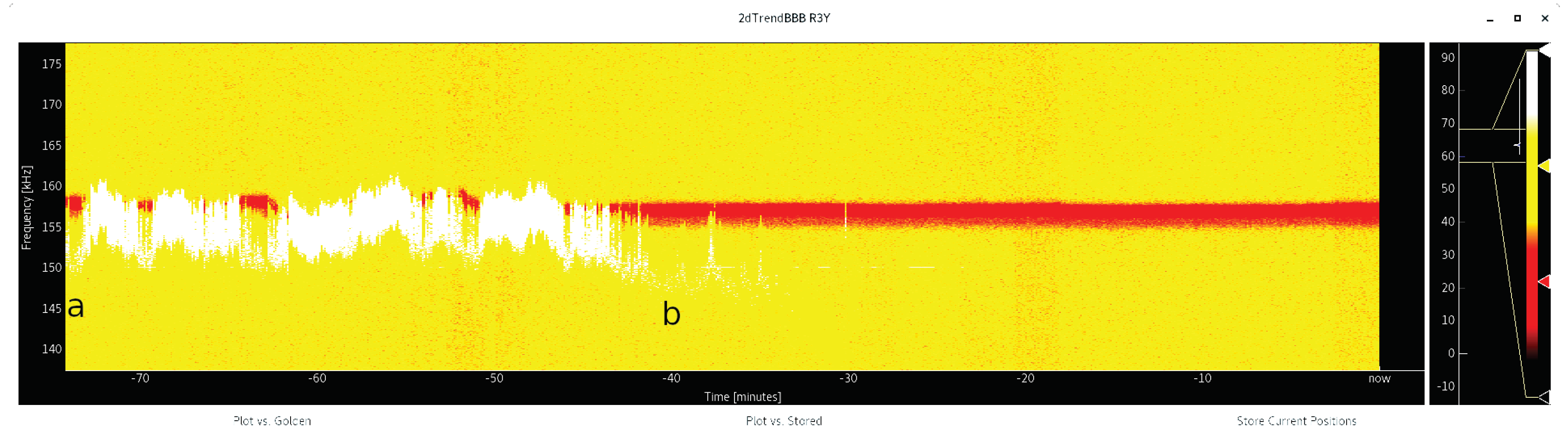
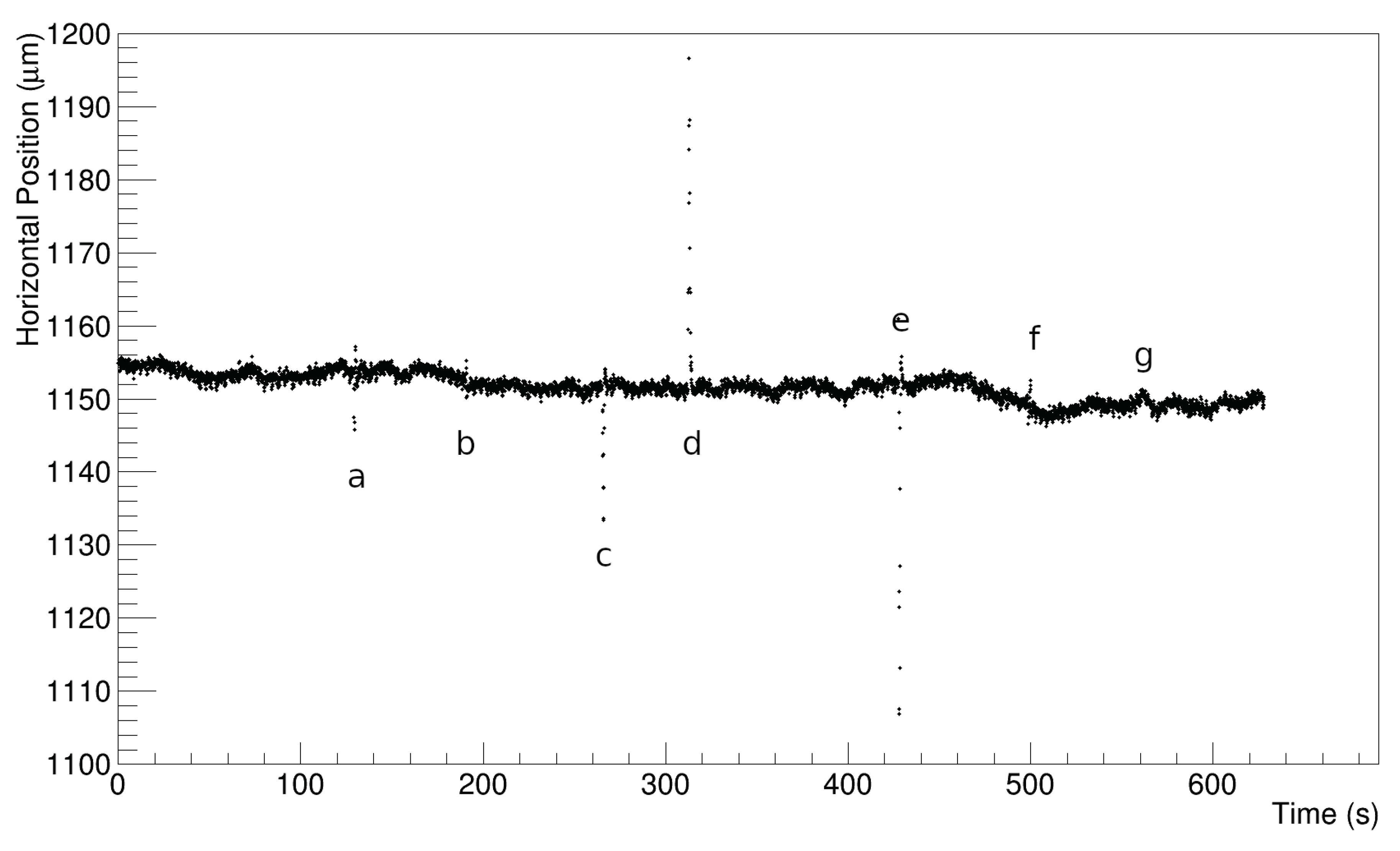
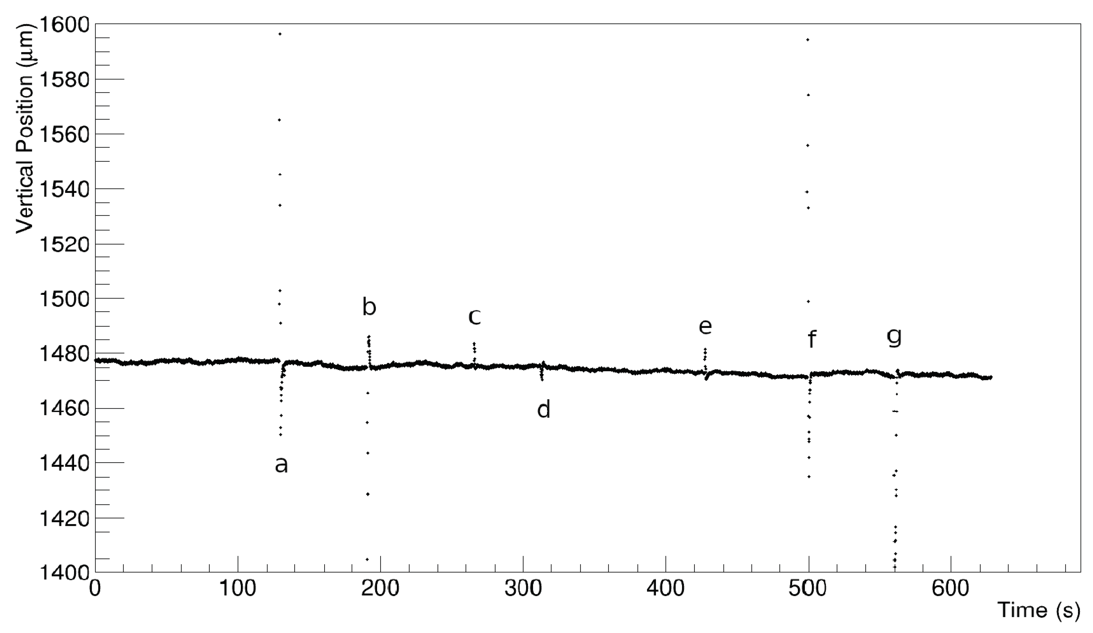
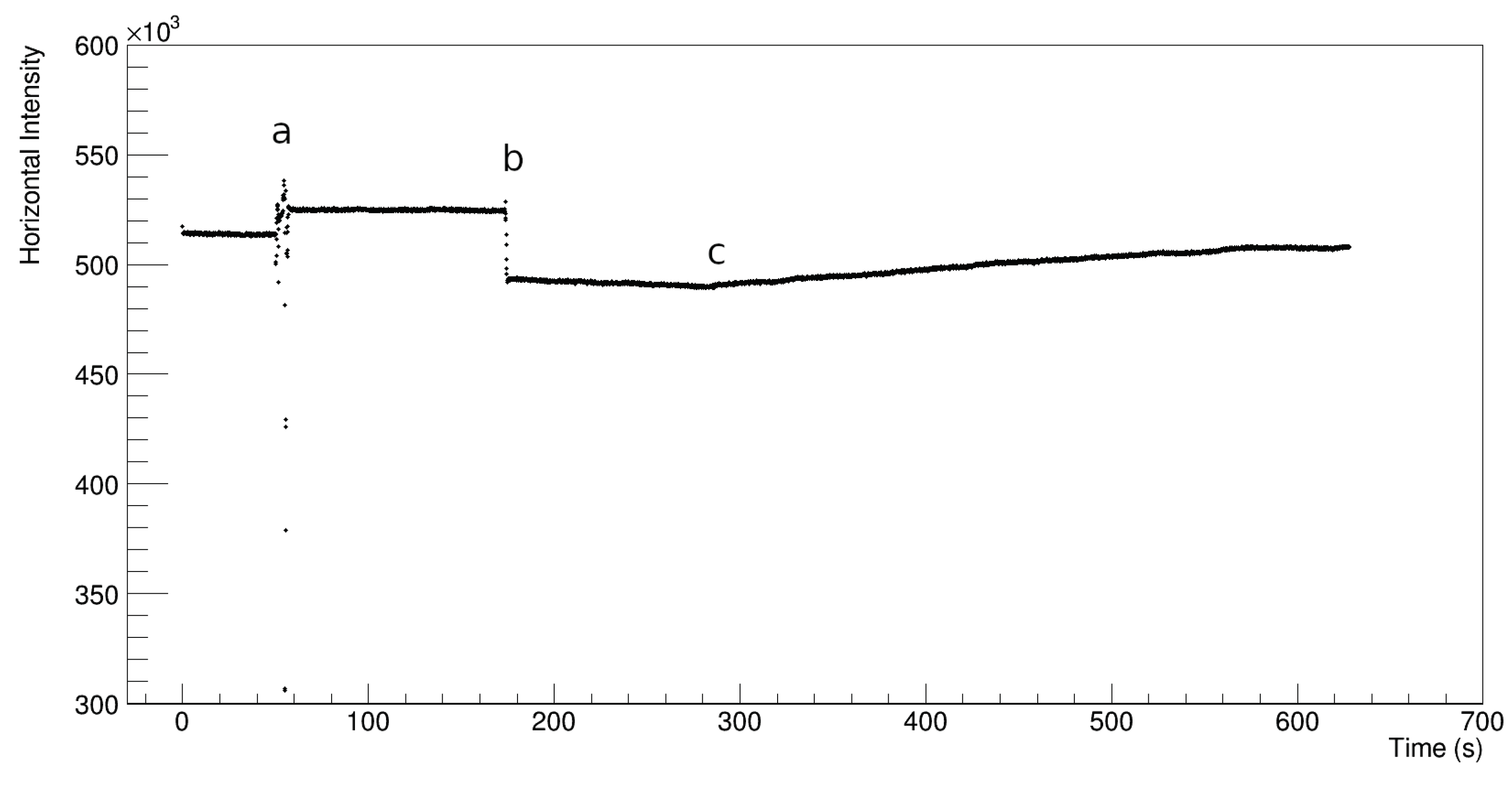
3. Beam Position Monitor Time Evolution

The Beam Position Monitor Time Evolution (BPM trends) [13] is a tool developed by the operations group that shows the storage rings’ beam positions over time (a real-time “sliding plot” during operations) as measured by all the rings’ BPMs. The vertical scale on the right (in μm) controls whether there is any deviation within the lower and upper limits set by the scale, where the histogram shown is a built-in PyQt function [14] showing the values for all plotted time points and BPMs for a given axis, which helps the user choose what range to look at. Figure 3 shows a typical example of stable delivery, where all BPM readings show the beam is kept within the required limits (within 0 μm to ±0.3 μm, in this case) and are therefore shown in green. When the deviation is above the upper limit (0.3 μm), the points are shown in red. An illustration of this fact is demonstrated in Figure 4, where one can observe that small changes to one of the beamline’s gaps in the 3 GeV storage ring can cause visible disturbances to the beam. In Figure 5, it is noticeable that during injections a large vertical line can be observed in the 1.5 GeV ring BPM trends, due to the significant disturbances caused by the dipole kicker that it is used in the smaller ring. A similar line is not observed in Figure 3 as the 3 GeV ring makes use of the MIK.
The tool allows also the possibility of switching mode between “BPM-space” and “corrector-space”, the former being the positions measured by the BPMs, with the latter being the BPM positions transformed through the orbit response matrix (ORM) to the angular kicks at the corrector magnets that would result in the observed orbit distortions. The ORM is normally used for the feedback system to calculate corrector magnet strengths, and, by the same logic, it is possible to use the ORM to locate where kicks on the beam are originating from.
Two-dimensional colormap spectrograms are also useful to monitor the synchrotron and betatron frequencies variations measured by the BBB system [8,9] and, therefore, a useful tool to monitor the accelerator’s tunes. At times, when there are disturbances of the same order as the frequency of the tunes, the spectrograms convey a clearer image than just observing the tune value. Figure 6 illustrates a typical use case. At approximately −40 min (point “a”), the MO RF of the 3 GeV storage ring is manually increased in an attempt to change the vertical tune closer to its delivery set value (0.265). The MO RF changes are done in 5 Hz steps, which is visible in the staircase decrease of the vertical betatron frequency. At −5 min (point “b”), one of the beamlines closes its undulator gap, causing the tune to shift, which is clearly visible at right end of the plot. An example of the use of this tool to diagnose faulty equipment is given in Figure 7. Between −80 (point “a”) and −40 min (point “b”), a disturbance can be seen around the tune frequency. At point “b”, a faulty amplifier connected to an alternative tune measurement system was turned off. This vertical disturbance caused an increase in vertical emittance, which decreased to nominal values as soon as the disturbance moved away from the tune frequency.
The tool also provides a good way to visualize whether the beam is behaving as expected in all planes of space. Figure 8 shows the longitudinal and transverse frequencies for the 1.5 GeV storage ring. In the longitudinal plane (synchrotron frequency, top plot), one can see the effects of the top-up injections every 30 min. In the vertical plane (middle plot), one can see the signal is strongest around 350 kHz, but lines for higher and lower frequencies, albeit weaker, can be seen, which is consistent with the synchrotron sidebands of the betatron frequency measured by the BBB system. A similar, but less pronounced, effect can be observed in the horizontal plane (bottom plot). Such plots can be constantly monitored during beam delivery, and should significant deviations on the shown patterns be observed in any of the planes, actions can be taken to improve beam quality and prevent beam losses.

4. WOBBL

Localized changes in the orbit at an insertion device causes a detectable change in the operating point of an accelerator; a feedback system can restore the beam trajectory to its desired orbit by modifying the strength of corrector magnets in order to compensate for the localized change; and the maximum measurable disturbance in the orbit can be controlled by limiting the amplitude of the localized change during the time constant of the feedback loop.
During normal operations at MAX IV, it is common for beamline users to request changes to the orbit of the beam through the long straight sections of the storage rings where the insertion devices are situated. The implementation of such orbit bumps is done by changing the reference orbit to which the SOFB corrects the beam. Manual implementation of a beamline bump results in an abrupt disturbance of the stored beam, which is not transparent to the users at the beamlines.
In order to accommodate beamline bump change requests without disturbing the measurements performed at any of the other beamlines, a Widget for setting the Orbit Bumps for BeamLines (WOBBL) [15] has been developed within the operations group. The WOBBL application is a python program utilizing the PyQt module’s QtGui to build a user interface. The internal timing system of the application relies on PyQt QtCore QTimer objects, which connects to a method for implementing changes to the beamline orbit bumps. Interaction with the machine is done by sending new reference orbit to the slow orbit feedback TANGO devices, which are part of a TANGO-based control system accessed through the pyTANGO module.
WOBBL implements changes to the reference positions for the SOFB in a series of sub-micrometer steps at a repetition rate which is lower than that of the feedback system; in other words, each step is small enough to not cause a too large perturbation on the beam and slow enough to allow the SOFB to correct orbit drifts. This allows the orbit to be corrected in-between each step change. The result is a smooth transition from the initial orbit to the desired final orbit.
Figure 9 shows the WOBBL interface which is used to implement the beamline orbit changes non-disruptively. The WOBBL interface shows the beamlines which are in normal operation for the 3 GeV ring and also the MIK. The widget has input fields for setting each of the four types of bump changes, for each beamline. Via the widget, it is also possible to get a read-back of the positions and angles through the insertion devices, as picked up by BPMs in the ring. Both the step size and repetition rate are available as input settings.
In order to determine the effectiveness of the WOBBL tool in a controlled manner, studies were performed for the NanoMAX [16] beamline, one of the most instability-sensitive beamlines at the MAX IV laboratory. Is is worth noticing that the positions and intensities are with respect to the X-ray beam and, therefore, provide a direct estimation of the impact of the tool for an experiment.
During the measurements, the bumps for another beamline (BioMAX [17]) were changed both directly and via the WOBBL tool and compared. Changes in the BioMAX bumps are performed also in order to test whether a bump change in a particular plane (e.g., vertical) for BioMAX are felt by NanoMAX in both horizontal and vertical planes or if predominately in the same plane where the change was performed.
Figure 10 shows the horizontal X-ray beam position observed by NanoMAX. Within the time scale of observations, when no bump changes are done, fluctuations of the order of ∼1 μ can be observed. Vertical changes in BioMAX bumps are done at points “a”, “b”, “f”, and “g”. It is clear that the direct vertical changes in BioMAX’s bumps do affect NanoMAX’s measured horizontal X-ray beam position. They are, however, significantly smaller than the large horizontal X-ray beam position displacements that are seen at points “c”, “d” and “e”. One can notice that, at point “d", in particular, a perturbation of ∼40 μ is measured. A consistent pattern can be seen in Figure 11, where the vertical beam position measured by NanoMAX is shown. The vertical bump changes done for BioMAX at points “a”, “b”, “f”, and “g” cause large perturbations, as large as ∼80 μ at point “g”, in NanoMAX’s measured vertical position, while the horizontal bump changes for BioMAX bumps implemented at points “c”, “d”, and “e” cause significantly smaller perturbations.
Figure 12 shows for comparison the horizontal X-ray beam position measured by NanoMAX, but, this time, changes are done at BioMAX’s bumps now using the WOBBL tool. Horizontal bump changes for BioMAX, which should most significantly affect the measured X-ray beam horizontal position, are done at t = 25 s (point “a”) and t = 385 s (point “b”). No significant disturbances in NanoMAX’s beam position can be observed during those changes. A similar plot for NanoMAX’s vertical position is not shown for concision reasons.

WOBBL Limitations and Future Improvements

WOBBL is a tool capable of making changes to the beam orbit through IDs of the 1.5 GeV and 3 GeV rings at MAX IV with sub-micrometer precision. Its current limitations in performance are partly set by the SOFB systems of he rings. The SOFB system determines how well the orbit can be corrected to the new reference positions set by the WOBBL tool. It also limits the maximum iteration rate which can be used while changing a beamline bump, as it has to be set lower than that of the orbit feedback system which is currently operating at 10 to 20 Hz. Both of these limitations are to be considered minor as a beamline bump can be implemented in less than a minute, in a way which is transparent to the other beamlines and without causing disturbances to the beam orbit which is outside of the specification of the ring. The tool is currently limited to changing one beamline bump at a time unless more than one instance of WOBBL is used, since it is a standalone application not integrated in the TANGO-based control system. Work to implement this integration has started. It will allow for archiving of the beamline orbit bumps and other benefits once it has been integrated with the rest of the control system. Simultaneously, an upgrade will be made to enable handling of multiple beamline bump changes at once, something which will be of greater importance as more beamlines are commissioned in the future.

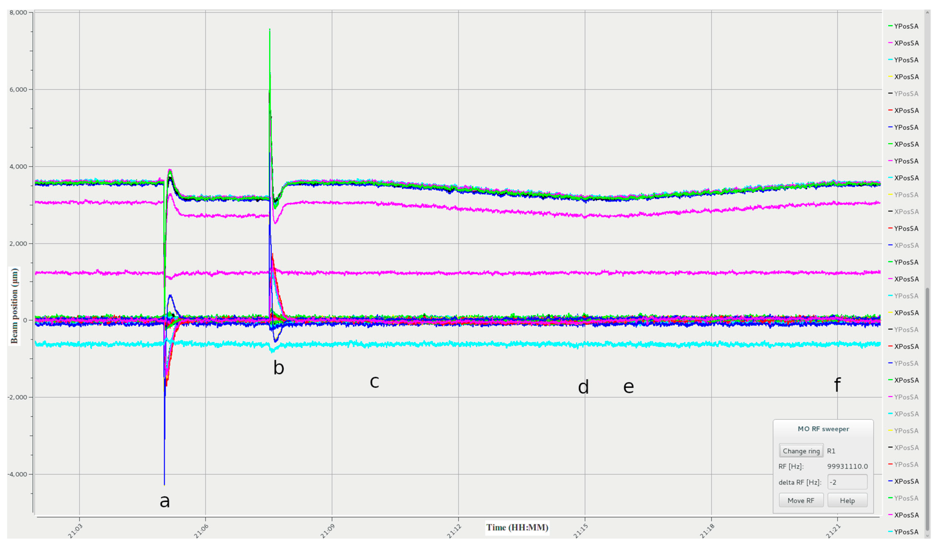
5. Soft MO RF Sweeper

The soft MO RF sweeper [18] is a tool for changing the MO RF of a storage ring in combination with an orbit feedback system. With this tool, changes in the MO RF can be carried out without significantly affecting beam instability-sensitive beamlines as the adjustments made in each step are carefully set up such that the beam instabilities arising from the MO RF adjustments are as small as the regular beam oscillations. Such regular oscillations can have several origins, such as small mechanical vibrations or coupled-bunch instabilities, and can of course also be caused by several types of beamline activities, such as changes in undulator gaps and phases. As with the WOBBL, each adjustment also gives time for the orbit feedback system to adjust the beam orbit after adjusting the MO RF. This is accomplished by fulfilling two conditions: (a) at least one second has to elapse and (b) at least five iterations of beam trajectory corrections have to be carried out before the next MO RF adjustment is done.
At the two MAX IV storage rings, it was found that MO RF adjustments of 0.05 Hz results are practically undetectable by beam instability-sensitive beamlines. The simple graphical user interface (GUI) of this tool shows which storage ring is selected, the current MO RF and the desired change of the MO RF. After activating the sweep, the MO RF is moved in steps of 0.05 Hz until the defined change has been accomplished or if stopped by the user.
In Figure 13, the difference between applying a change of 5 Hz directly and via the soft MO RF sweeper is visible from the 1.5 GeV storage ring beam data. At time instants when the MO RF is directly increased by 5 Hz ( point “a”) and decreased by 5 Hz ( point “b”), a large deviation in beam position is measured by the 1.5 GeV storage ring BPMs, both in the vertical and horizontal planes. Between points “c” and “d”, the same 5 Hz increase is applied to the MO RF, followed by a 5 Hz decrease between points “e” and “f”, both via the sweeper-disturbances to the beam orbit are then barely seen. This preservation of stability that is accomplished with the MO RF sweeper is crucial during delivery for the experiments measurements to be carried out without disturbances.
As with the WOBBL tool, the effect can be observed for NanoMAX, at t = 50 s ( point “a”), that the MO RF is increased directly by 5 Hz, which can be observed (Figure 14) at NanoMAX’s measured beam horizontal intensity, which is basically the X-ray beam intensity (for the calculation of the horizontal and vertical beam position (and intensity), a 2D image of the x-ray beam profile is summed, with he resulting beam profile fitted with a Gaussian function - as it is the fitted amplitude, and not the actual maximum intensity, the vertical and horizontal beam intensities can differ). The effect is also clearly visible at the horizontal X-ray beam position (Figure 15). The beam intensity abruptly decreases X-ray beam position oscillates as much as ∼150 μm (a similar effect is observed in the vertical plane, but is not shown). At t = 174 s ( point “b”), the MO RF is decreased by 10 Hz directly and once more a large disturbance in the delivered beam for NanoMAX is observed for both quantities. At 285 s ( point “c”), the MO RF starts to be increased towards a total 5 Hz change using the sweeper. The effect is observable as a subtle drop in the horizontal intensity in Figure 14 at point “c”, which starts increasing again during the approximate 5 min it takes the MO RF to reach its new desired value. The change is not noticeable in the horizontal X-ray beam position in Figure 15 at the same point in time. In summary, a MO RF change is significantly noticeable by NanoMAX (at points “a” and “b”) when a direct change is performed and is barely noticeable as a slight decrease in intensity when the sweeper is used (point “c”), which is a strong indicator of the sweeper’s usefulness during beam delivery.

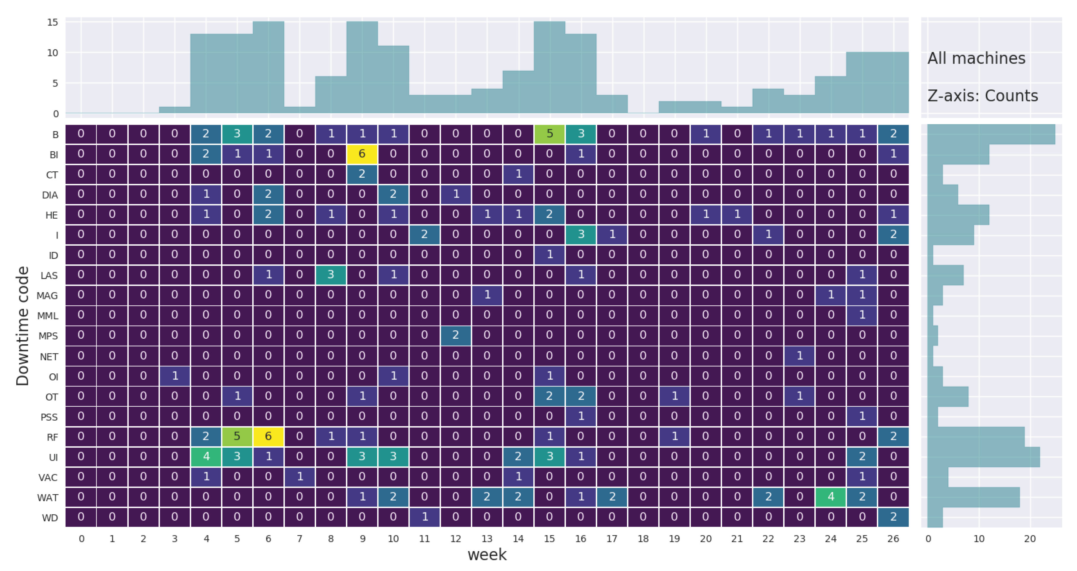
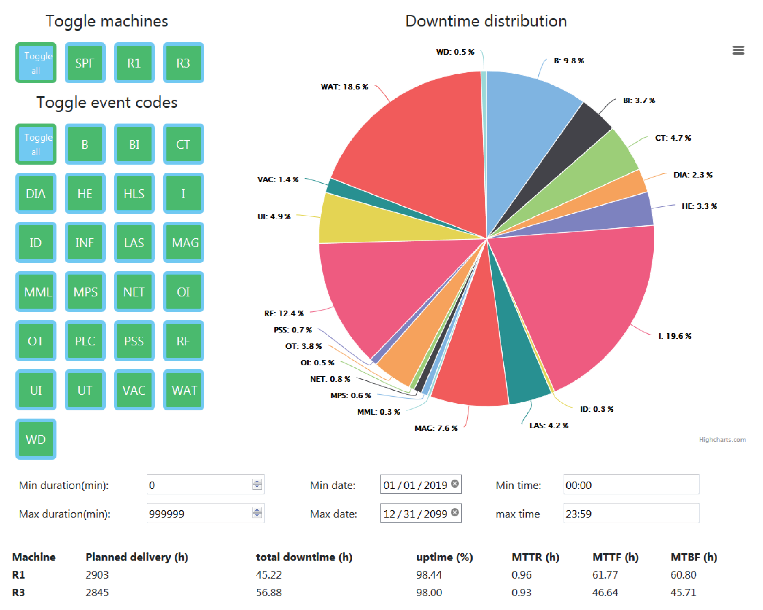
6. Availability and Downtime Monitoring

The tracking of machine downtime duration with subsequent determination of causes is a crucial technique that is used to maximize reliability in complex systems. At MAX IV a “downtime web-application” was developed [19] for such purpose. The application handles client server communication in Javascript using Node JS. The page rendering uses the HTML template engine Pug, which let the user write webpages using an easy to read indentation based syntax. The downtime events are stored using the database framework MongoDB. The database can be browsed from any device on the MAX IV network via the DowntimeApp. At MAX IV, the write access is restricted to members of the operations group.
The application allows one to easily edit and add accelerator operations schedules and report any unscheduled downtime to a database. For each downtime event, a machine (the Linac (I), the 3 GeV (R3) or the 1.5 GeV (R1) storage rings) is indicated together with an event type code, the date and time of the day, the downtime’s duration and the name of the reporting operator together with a description of what happened. The application then uses the schedule and the downtime events to calculate Mean Time Between Failures (MTBF), Mean Time To Failure (MTTF), and Mean Time to Repair (MTTR) on timescales controlled by the user. It also allows easy visualization of downtime duration by machine (R1, R3, I) or event label, which can be beamlines, beam instability, controls, diagnostics, human error, high level software, injector, insertion devices, infrastructure, laser (photo-cathode gun), magnets, machine protection system, network, orbit interlock, programmable logic controller, personnel safety system, radio frequency, vacuum, water, WatchDog (software), or others, if the cause is unknown or no existing label is well suited.
The database can be downloaded as a CSV file and analyzed in further detail. The heatmap in Figure 16 shows number of downtime events by code and week number for all three systems (I, R3, R1). The histograms on the margins are the projections of the heatmap onto the x and y-axis. The histogram on the right margin shows that certain event types are more frequent, and the upper histogram highlights how the downtime is distributed across the run period. The heatmap in Figure 17 shows the distribution of downtime events across days and hours (the hour during which the downtime started). The upper histogram shows that downtime is more likely to occur during daytime. This is likely because there are more users during this time, which leads to more parameters changing in the machines. During the spring run period of 2019, Tuesdays were designated as maintenance days, which entailed little or no delivery. The histogram on the right margin shows that Monday and Wednesday are the days with the most downtime events, while the number of events decreases as the week progresses. We conclude from this that downtime is more frequent on Mondays, when people resume their activities after the weekend, and on Wednesdays, when we have a complete restart of activities following the maintenance day. To minimize downtime, as well as to maximize the efficiency of machine studies periods, the maintenance days have thus been moved to Mondays starting in the Autumn run of 2019.
Figure 18 shows that a beam availability of 98.4% was achieved for the 1.5 GeV storage ring (with 60h of MTBF) and of 98.0% for the 3 GeV ring (with 40h of MTBF) during the first half of 2019. This can be compared to a beam availability of 96.7% for the 1.5 GeV storage ring (with 59.6 h of MTBF) and of 96.2% for the 3 GeV ring (with 34.5 h of MTBF) during 2018. The straightforwardness in which those numbers, as well as as the analyses plots, can be obtained with the application have an important influencing factor for accelerator operations policies.

7. Discussion

While different laboratories can have their own accelerator tools to accomplish similar goals to the ones described in this article, direct and quantitative information of the impact of these accelerator control applications to an experiment is provided using X-ray beam data (Section 4 and Section 5). This is important because synchrotron light facilities, such as MAX IV, are measured by the quality of light they produce. The improvement provided by the tools can also be, to some extent, inferred by the increase in uptime from 2018, when the tools were under development, to 2019, when these became standard tools in the MAX IV accelerator operations. Furthermore, real time diagnostics of problems is one of the main goals of accelerator operations, not limited to, but principally, during user operations. The BPM trends tool is one of the most useful tools for this purpose, allowing, for example, the deduction of problems with orbit corrections, even when other systems point to it be running without problems. As it became so successful at MAX IV, we present it as an additional, freely distributed, diagnostic instrument that other laboratories might find useful to test. Finally, other solutions to logging systems, similar to the presented Downtime application, of course exist. One such example is the “Operation event logging system of the Swiss Light Source” [20]. It is, however, not the goal of the present article to provide a comparison but to share our own results, provide it as an alternative solution, and freely distribute it for the benefit of the accelerator community.

8. Conclusions

Several applications developed by the MAX IV accelerator operations group were presented. Most of the tools are for monitoring purposes, but the group also developed software that directly improved the beam stability seen by the beam users. Specifically, the following software tools were presented: (i) a tool which displays the beam position’s evolution over time and the accelerator tunes’ evolution, (ii) a tool that reduces the impact of changing orbit bumps for the beamlines, (iii) an application for adjusting the master oscillator’s radio-frequency of a storage ring that is nearly transparent for users, and (iv) the downtime web-application used for registering and monitoring the availability and downtime of accelerators. The development of these programs significantly improved accelerator operations at the MAX IV laboratory. All tools are provided with public links to the code repositories and can be used by other groups at other facilities, in particular, at synchrotron radiation laboratories making use of TANGO-based control systems.

Author Contributions

Conceptualization, B.M.; Methodology, B.M.; Software, R.H., B.B., A.J., J.P., J.E.P., R.S.; Formal Analysis, B.M.; Investigation, B.M., S.K.; Data Curation, B.M.; Writing—Original Draft Preparation, B.M., B.E.B., R.H., A.J., S.M., J.E.P.; Writing—Review & Editing, B.M., V.A., F.B., M.B., M.H., P.L., J.S.L., F.P., H.S., R.S., D.W. All authors have read and agreed to the published version of the manuscript.

Funding

The work reported in this paper was fully funded by MAX IV Laboratory.

Conflicts of Interest

The authors declare no conflict of interest.

References

  1. Martensson, N.; Eriksson, M. The saga of MAX IV, the first multi-bend achromat synchrotron light source. Nucl. Instrum. Methods Phys. Res. 2018, 907, 97–104. [Google Scholar] [CrossRef]
  2. Fernandes Tavares, P.; Leemann, S.; Sjöström, M.; Andersson, Å. The MAX IV storage ring project. J. Synchrotron Radiat. 2014, 21, 862–877. [Google Scholar] [CrossRef] [PubMed] [Green Version]
  3. Tavares, P.; Al-Dmour, E.; Andersson, Å.; Breunlin, J.; Cullinan, F.; Mansten, E.; Molloy, S.; Olsson, D.; Olsson, D.; Sjöström, M.; et al. Status of the MAX IV Accelerators. In Proceedings of the 10th International Particle Accelerator Conference (IPAC2019), Melbourne, Australia, 19–24 May 2019; p. TUYPLM3. [Google Scholar] [CrossRef]
  4. Kallestrup, J.; Alexandre, P.; Andersson, Å.; Ben El Fekih, R.; Breunlin, J.; Olsson, D.; Tavares, P. Studying the Dynamic Influence on the Stored Beam From a Coating in a Multipole Injection Kicker. In Proceedings of the 10th International Particle Accelerator Conference (IPAC2019), Melbourne, Australia, 19–24 May 2019; p. TUPGW063. [Google Scholar] [CrossRef]
  5. Tavares, P.F.; Andersson, Å.; Hansson, A.; Breunlin, J. Equilibrium bunch density distribution with passive harmonic cavities in a storage ring. Phys. Rev. ST Accel. Beams 2014, 17, 064401. [Google Scholar] [CrossRef]
  6. Salom, A.; Andersson, Å.; Lindvall, R.; Malmgren, L.; Milan, A.; Mitrovic, A.; Pérez, F. Digital LLRF for MAX IV. In Proceedings of the 8th International Particle Accelerator Conference (IPAC 2017), Copenhagen, Denmark, 14–19 May 2017; p. THPAB135. [Google Scholar] [CrossRef]
  7. McGinnis, D.P. Beam Stabilization and Instrumentation Systems based on Internet of Things Technology. In Proceedings of the Low-Level Radio Frequency Workshop (LLRF 2019), Chicago, IL, USA, 29 September–3 October 2019. [Google Scholar]
  8. Olsson, D.; Malmgren, L.; Karlsson, A. The Bunch-by-Bunch Feedback System in the MAX IV 3 GeV Ring; Technical Report LUTEDX/(TEAT-7253)/1-48/(2017); MAX-lab, Lund University: Lund, Sweden, 2017; Volume 7253. [Google Scholar]
  9. Olsson, D.; Andersson, Å.; Cullinan, F.; Tavares, P. Commissioning of the Bunch-by-Bunch Feedback System in the MAX IV 1.5 GeV Ring. In Proceedings of the 9th International Particle Accelerator Conference (IPAC 2018), Vancouver, BC, Canada, 29 April–4 May 2018; p. THPAL028. [Google Scholar] [CrossRef]
  10. Ahlback, J.; Johansson, M.A.G.; Leemann, S.C.; Nilsson, R.; Sjöström, M. Orbit Feedback System for the MAX IV 3 GeV Storage Ring. Conf. Proc. 2011, C110904, 499–501. [Google Scholar]
  11. Leemann, S.; Andersson, Å.; Sjöström, M. First Optics and Beam Dynamics Studies on the MAX IV 3 GeV Storage Ring. In Proceedings of the 8th International Particle Accelerator Conference (IPAC 2017), Copenhagen, Denmark, 14–19 May 2017; p. WEPAB075. [Google Scholar] [CrossRef]
  12. Thorin, S.; Andersson, J.; Curbis, F.; Eriksson, M.; Karlberg, O.; Kumbaro, D.; Mansten, E.; Olsson, D.; Werin, S. The MAX IV Linac. In Proceedings of the 27th Linear Accelerator Conference, LINAC2014, Geneva, Switzerland, 31 August–5 September 2014; pp. 400–403. [Google Scholar]
  13. Petersson, J.; Svärd, R. BPM-Trends. 2019. Available online: https://github.com/hurvan/BPM-Trends (accessed on 25 August 2020).
  14. PyQtGraph. Available online: https://pyqtgraph.readthedocs.io/en/latest/graphicsItems/histogramlutitem.html (accessed on 25 August 2020).
  15. Johansson, A. WOBBL—Widget for Orbit Bumps at BeamLines. 2019. Available online: https://gitlab.com/maxivOperations/wobbl/-/tree/master (accessed on 25 August 2020).
  16. Johansson, U.; Vogt, U.; Mikkelsen, A. NanoMAX: A hard x-ray nanoprobe beamline at MAX IV. In X-ray Nanoimaging: Instruments and Methods; SPIE: San Diego, CA, USA, 2013; Volume 8851, p. 88510L. [Google Scholar] [CrossRef]
  17. Thunnissen, M.; Sondhauss, P.; Wallén, E.; Theodor, K.; Logan, D.; Labrador, A.; Unge, J.; Appio, R.; Fredslund, F.; Ursby, T. BioMAX: The Future Macromolecular Crystallography Beamline at MAX IV. In Proceedings of the 11th International Conference on Synchrotron Radiation Instrumentation (SRI 2012), Lyon, France, 9–13 July 2012; Volume 425. [Google Scholar] [CrossRef]
  18. Bolling, B. Soft Master Oscillator Radio Frequency Sweeper. 2019. Available online: https://github.com/benjaminbolling/MAXIVsoftRFsweeper (accessed on 25 August 2020).
  19. Høier, R. MAX IV Downtime Web Application. 2019. Available online: https://github.com/Rasmuskh/downtime (accessed on 20 August 2020).
  20. Lüdeke, A. Operation event logging system of the Swiss Light Source. Phys. Rev. ST Accel. Beams 2009, 12, 024701. [Google Scholar] [CrossRef] [Green Version]
Figure 1. MAX IV floor plan showing beamlines and the storage rings.
Instruments 04 00026 g001
Figure 2. MAX IV status page on 7 November 2019.
Instruments 04 00026 g002
Figure 3. Beam position monitor (BPM) trends in the horizontal plane for the 3 GeV storage ring during stable-beam delivery. The vertical axis displays the BPM number, while the horizontal axis displays the time (in minutes). The green points indicate that fluctuations in the horizontal beam position remained within the set tolerance of ±0.3 μm. The vertical scale on the right (in μm) controls whether there is any deviation within the lower and upper limits set by the scale.
Instruments 04 00026 g003
Figure 4. BPM trends in the horizontal plane for the 3 GeV storage ring. The vertical axis displays the BPM number, while the horizontal axis displays the time (in minutes). The vertical red lines are due undulator gap movements from a beamline. At these instants, the fluctuation of the beam position surpassed the set tolerance of ±0.3 μm. The vertical scale on the right (in μm) controls whether there is any deviation within the lower and upper limits set by the scale.
Instruments 04 00026 g004
Figure 5. BPM trends in the horizontal (top) and vertical (bottom) planes for the 1.5 GeV storage ring. The vertical axis displays the BPM number, while the horizontal axis displays the time (in minutes). The thick vertical red lines seen in both planes are due to dipole kicker top-up injections, indicating large perturbations in the beam’s position, both in the horizontal and vertical planes.
Instruments 04 00026 g005
Figure 6. The figure shows in the vertical axis the oscillation frequency (in kHz) in the vertical plane as measured by the BBB system as a function of time in the horizontal axis (in minutes). Starting approximately at −40 min (point “a”), the Master Oscillation (MO) radio frequency (RF) of the 3 GeV storage ring is manually increased in steps of 5 Hz is in order to change the vertical betatron tune. At −5 min (point “b”), one of the beamlines closes its undulator gap, which causes a visible perturbation.
Instruments 04 00026 g006
Figure 7. Accelerator tunes visualization in the 3 GeV storage ring. Between −80 (point “a”) and −40 min (point “b”), a disturbance can be seen around the tune frequency. At –40 min, a faulty amplifier connected to a tune measuring system was turned off. This vertical disturbance caused an increase in vertical emittance, which decreased to nominal values as soon as the disturbance moved away from the tune frequency.
Instruments 04 00026 g007
Figure 8. The longitudinal and transverse frequencies for the 1.5 GeV storage ring. In the longitudinal plane (synchrotron frequency), one can see the effects of the top-up injections (top plot). In the vertical plane (middle plot), one can see the signal is strongest around 390 kHz, but lines for higher and lower frequencies, albeit weaker, can be seen for higher and lower frequencies. A similar, but less pronounced, effect can be observed in the horizontal plane (bottom plot).
Instruments 04 00026 g008
Figure 9. Widget for setting the Orbit Bumps for BeamLines (WOBBL) interface containing the beamlines which are in normal operation for the 3 GeV ring and also the Multipole Injection Kicker (MIK). The widget has input fields for setting each of the four types of bump changes, for each beamline.
Instruments 04 00026 g009
Figure 10. Horizontal X-ray beam position observed by NanoMAX. The points where large perturbations (points “c”, “d”, and “e”) are observed, correspond to direct bump changes performed in the same plane for the BioMAX beamline. See main text for details.
Instruments 04 00026 g010
Figure 11. Vertical position observed by NanoMAX. The points where large perturbations are observed (points “a”,“b”,“f”, and “g”), correspond to direct bump changes performed in the same plane for the BioMAX beamline. See main text for details.
Instruments 04 00026 g011
Figure 12. Horizontal X-ray beam position measured by NanoMAX. Changes of the BiomaX bumps at done at points “a” and “b” using the WOBBL tool. No significant perturbations can be observed due to the applied changes. See main text for details.
Instruments 04 00026 g012
Figure 13. The soft Master Oscillator RF in use. The vertical axis displays the beam position (in μm) for several BPMs (represented by various colors), while the vertical axis displays the time (in HH:MM format). The MO RF is increased directly by 5 Hz at the marked point “a” and decreased by the same amount at point “b”. An increase by 5 Hz is than performed between points “c” and “d”, followed by a 5 Hz decrease between points “e” and “f”. The tool’s graphical user interface (GUI) can be seen in the bottom-right corner.
Instruments 04 00026 g013
Figure 14. NanoMAX’s horizontal beam intensity. At t = 50 s ( point “a”), the MO RF is increased directly by 5 Hz. The beam intensity decreases abruptly and significantly before rising again, as a result of MO RF increase. At t = 174 s ( point “b”), the MO RF is decreased by 10 Hz directly, and, once more, a large disturbance in the delivered beam for NanoMAX is observed. At 285 s ( point “c”), the MO RF starts to be increased towards a total 5 Hz change using the sweeper. The effect is observable as a subtle drop in the horizontal intensity at the recorded change time, which starts increasing again during the approximate 5 min it takes the MO RF to reach its new desired value.
Instruments 04 00026 g014
Figure 15. NanoMAX’s horizontal beam position. At t = 50 s ( point “a”), the MO RF is increased directly by 5 Hz. The horizontal X-ray beam position oscillates as much as ∼150 μm as a result of MO RF increase. At t = 174 s (point “b”), the MO RF is decreased by 10 Hz directly, and, once more, a large disturbance in the delivered beam for NanoMAX is observed. At 285 s ( point “c”), the MO RF starts to be increased towards a total 5 Hz change using the sweeper, which takes approximately 5 min, but the change is not noticeable in the plot.
Instruments 04 00026 g015
Figure 16. Heatmap of downtime at MAX IV as a function of event code and week number for all three machines (I, R3, R1).
Instruments 04 00026 g016
Figure 17. Heatmap of downtime at MAX IV as a function of days and start hour for all three machines (I, R3, R1).
Instruments 04 00026 g017
Figure 18. The front page of the downtime web-application.
Instruments 04 00026 g018
Table 1. Feedback systems used in the MAX IV storage rings.
Devices
Main cavity field amplitude and phase
Main cavity frequency
Landau cavity field amplitude
Robinson mode feedback (only 3 GeV ring)
Slow orbit feedback
Tune feedback (only 1.5 GeV ring)
Table 2. Nominal operations conditions for the 1.5 GeV storage ring.
ParameterValue
Stored current500 mA
Top-up mode30 min via dipole kicker
Filling patternUniform (32 buckets)
Landau cavities conditions2 cavities tuned in
BBB feedbackON (vertical and horizontal)
Slow orbit feedbackON
Table 3. Nominal operations conditions for the 3 GeV storage ring.
ParameterValue
Stored current250 mA
Top-up mode10 min via MIK
Filling pattern166/176 filled buckets
Landau cavities conditions3 cavities tuned in
BBB feedbackON (vertical)
Slow orbit feedbackON

