The Electric Field Detector on Board the China Seismo Electromagnetic Satellite—In-Orbit Results and Validation

 ,
,  , , , , , ,
Abstract
:1. Introduction
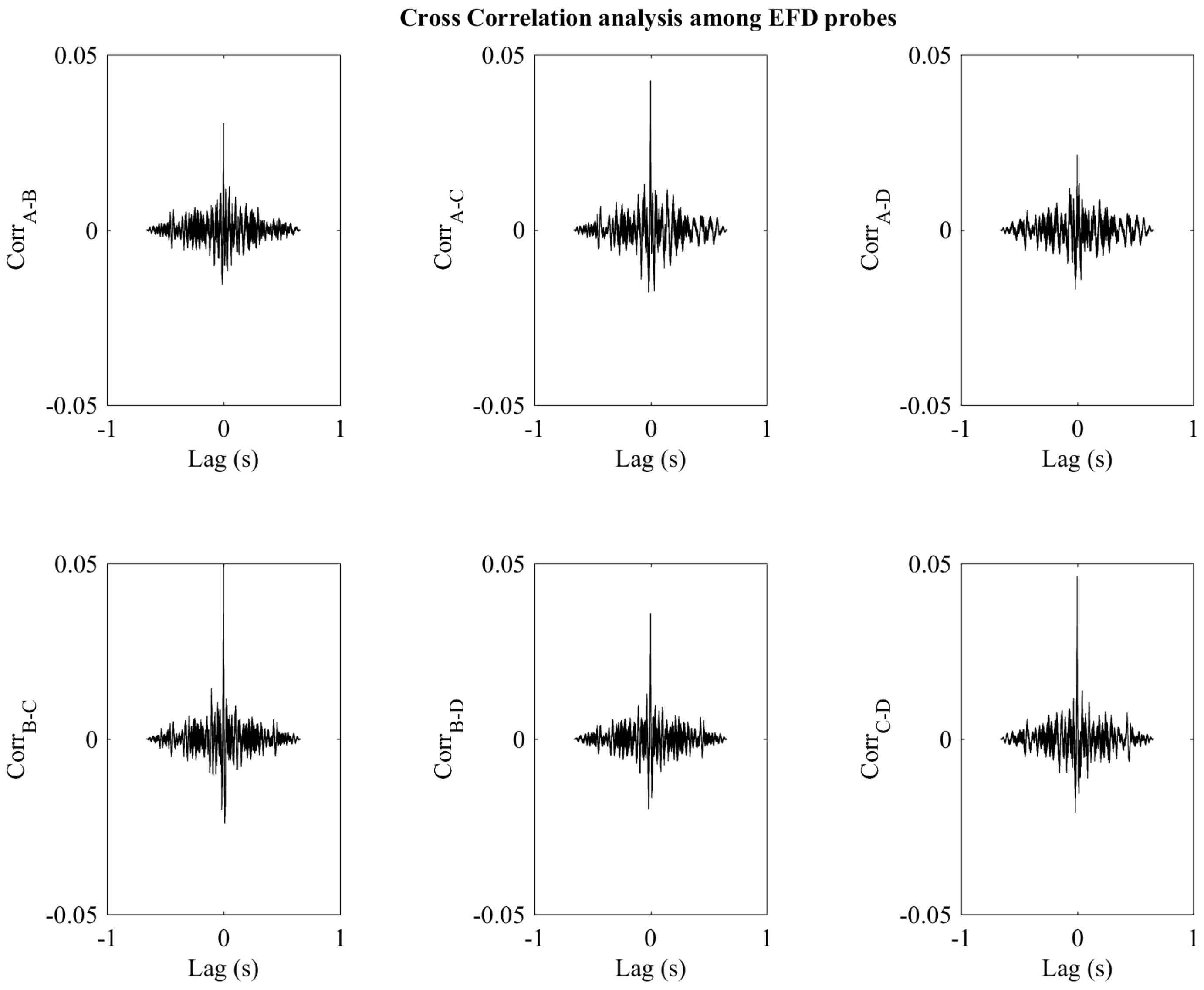
- = − ,
- = − ,
- = − .
2. Comparison between Expected and Measured Electric Field Values.
2.1. Quiet Condition
2.2. Perturbed Condition
3. EFD Capability in Observing Natural/Artificial Electromagnetic Signals
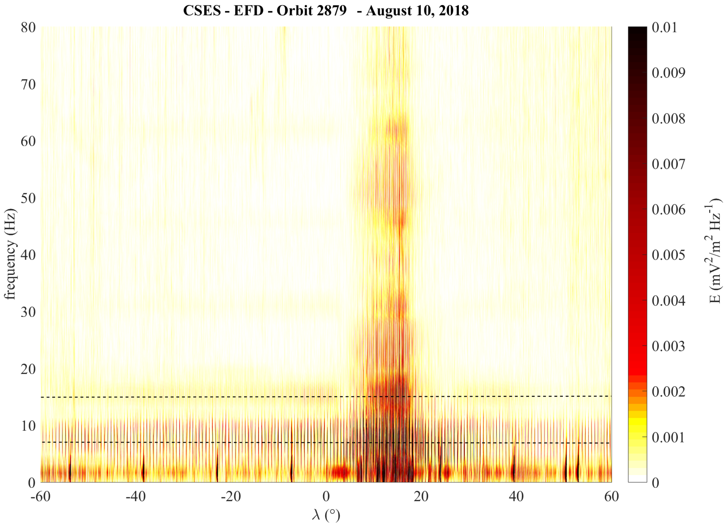
3.1. Schumann Resonance
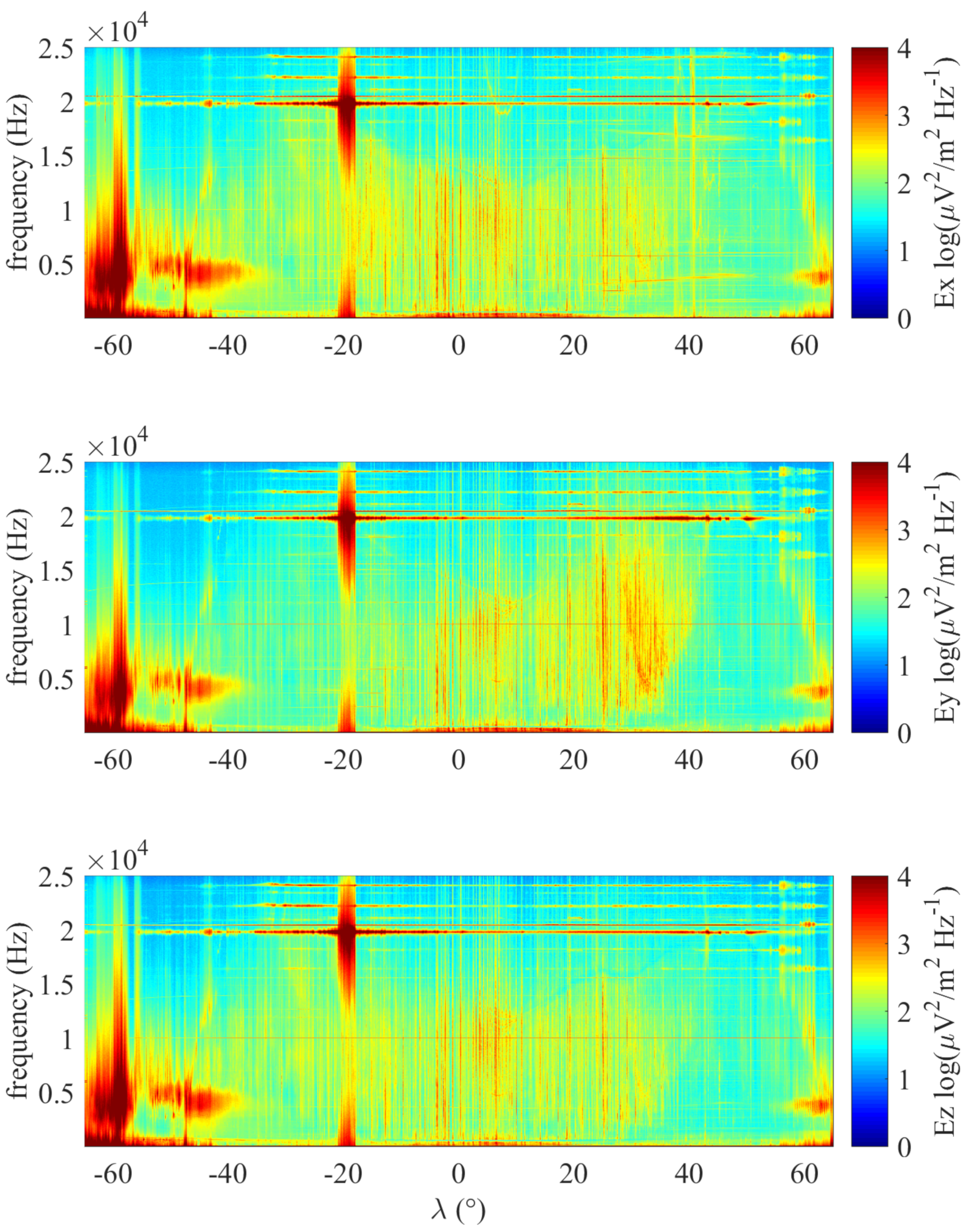
3.2. VLF Radio-Waves
4. Discussion
5. Conclusions
- 1.
- Comparison between and .
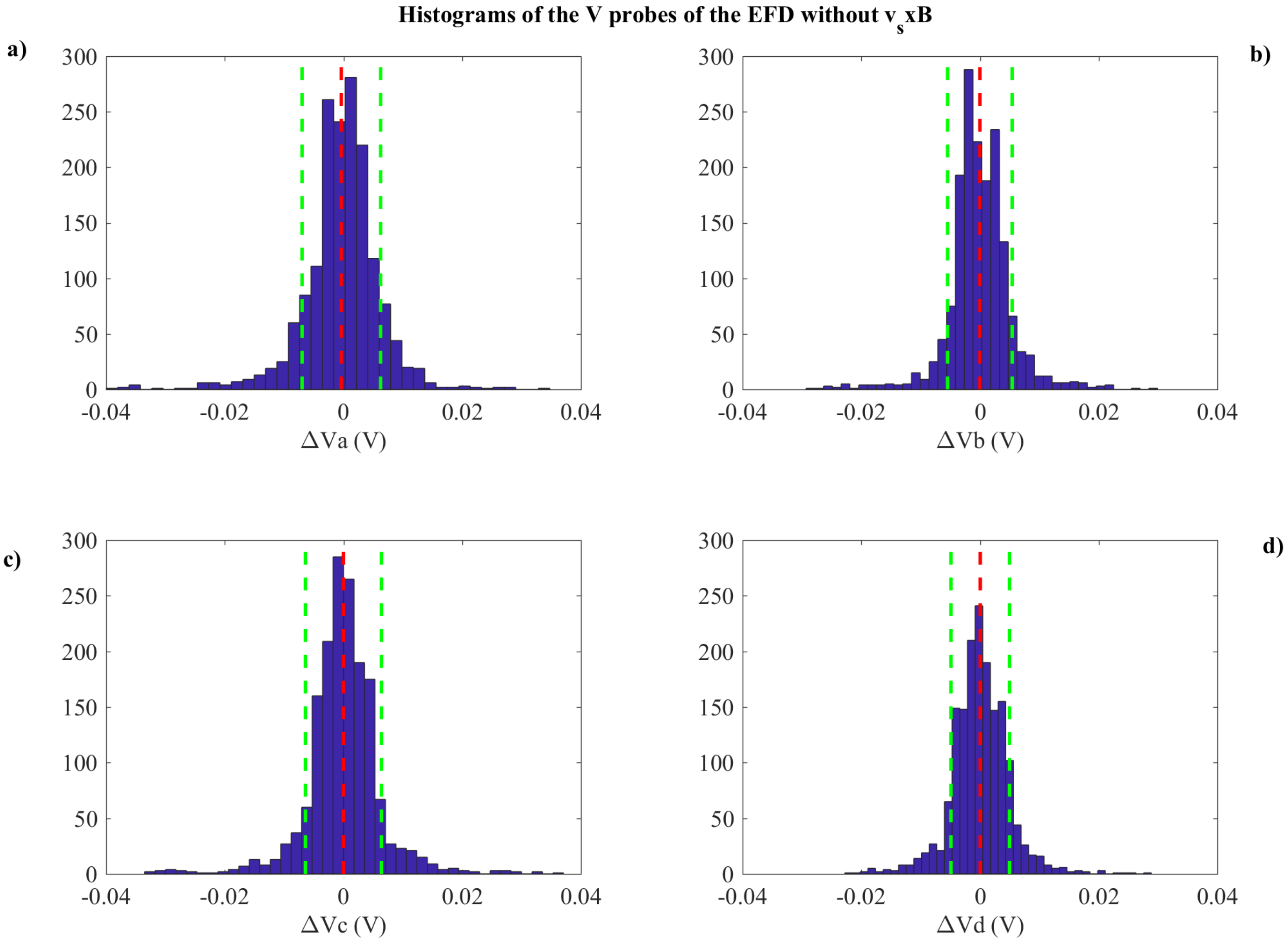
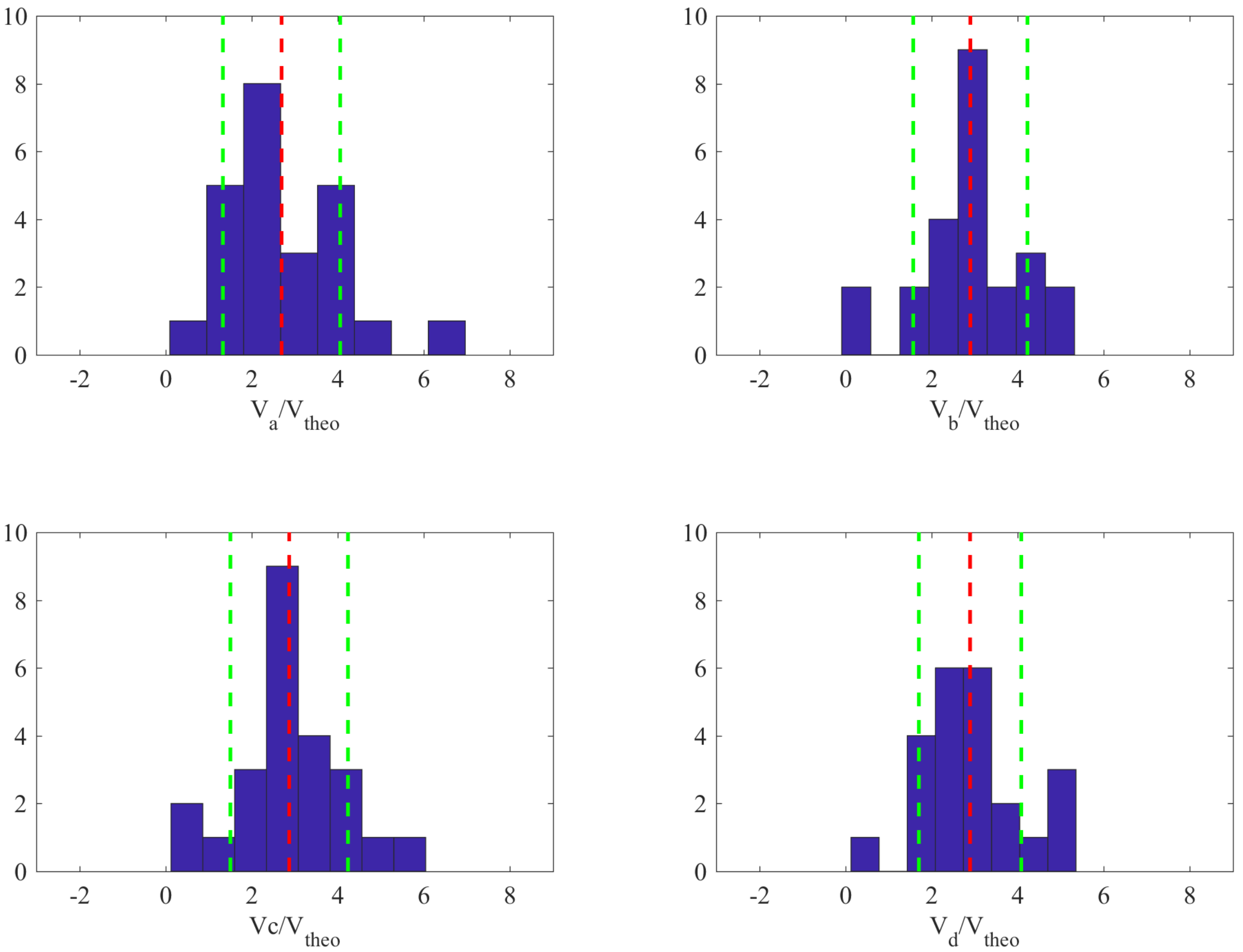
- Quiet conditions: the results demonstrate the reliability and consistency of both CSES LAP and EFD data. In fact, the difference measured between the four and the using the LAP density and the temperature observations (Figure 4), show average values lower than 1 mV.
- Perturbed conditions: because of the presence of a strong electric field altering the isotropic electrons collection, the OML theory is no longer valid and thus the results are uncertain due to the change in the actual probes collecting surface. As a consequence, we can only verify that the distributions shift is in the right direction and in the expected range as derived by the geometrical considerations.
- 2.
- Electromagnetic signals detection capability
- EFD shows a very good sensitivity resulting in the observation of the first peaks of the ionospheric Schumann resonance, which is a common phenomenon in the electric field data set, despite their very low amplitude.
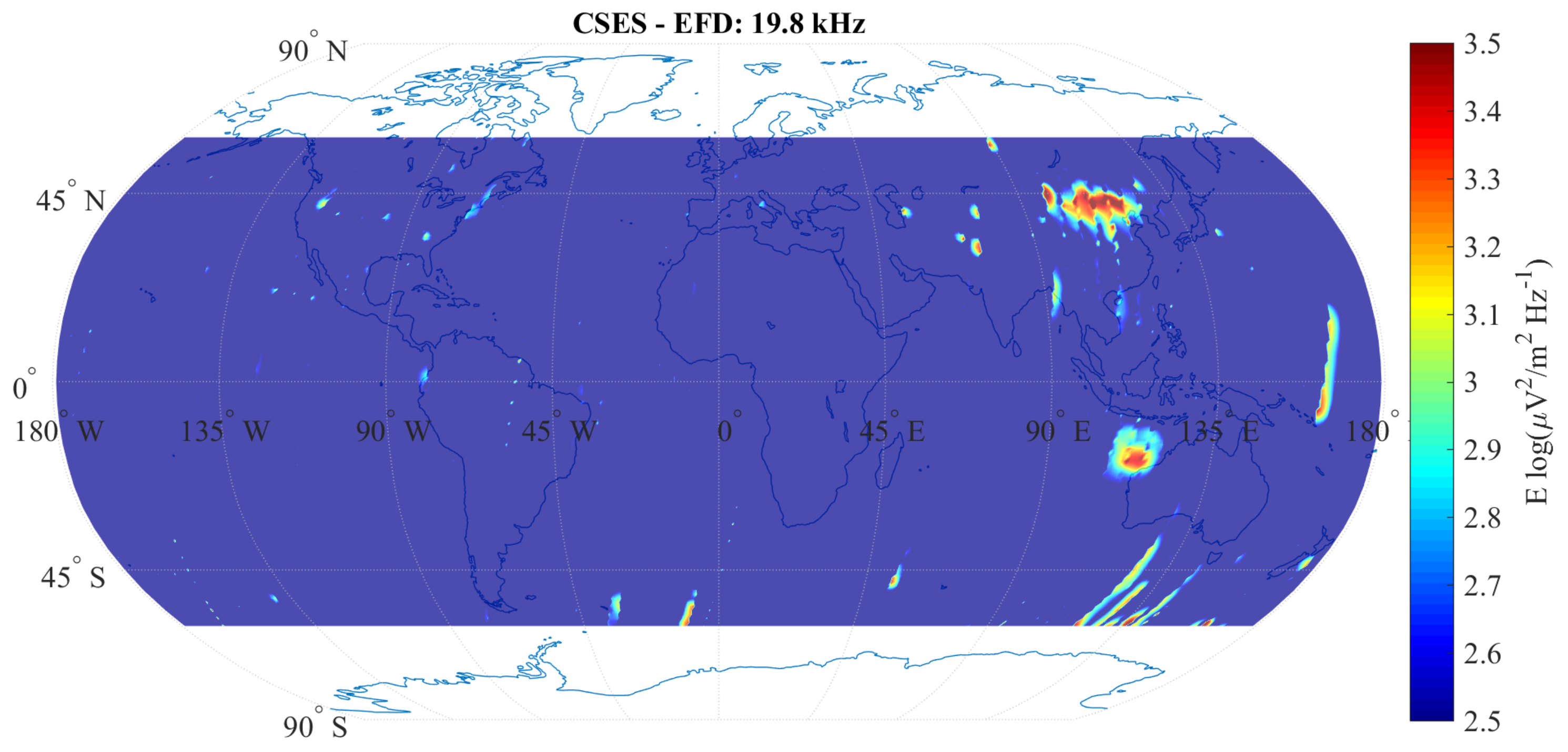
- CSES-01 satellite observed stable and reliable electromagnetic field enhancement excited by the NWC VLF transmitters whose peaks coincide with the crossing point of the magnetic force line from the bottom of the ionosphere to the conjugate region. Such a phenomenon confirms the ducted mode propagation of these VLF waves.
Author Contributions
Funding
Data Availability Statement
Acknowledgments
Conflicts of Interest
References
- Shen, X.; Zhang, X.; Yuan, S.; Wang, L.; Cao, J.; Huang, J.; Zhu, X.; Piergiorgio, P.; Dai, J. The state-of-the-art of the China Seismo-Electromagnetic Satellite mission. Sci. China Ser. E Technol. Sci. 2018, 61, 634–642. [Google Scholar] [CrossRef]
- Huang, J.; Lei, J.; Li, S.; Zeren, Z.; Li, C.; Zhu, X.; Yu, W. The Electric Field Detector (EFD) onboard the ZH-1 satellite and first observational results. Earth Planet. Phys. 2018, 2, 469–478. [Google Scholar] [CrossRef]
- Diego, P.; Bertello, I.; Candidi, M.; Mura, A.; Vannaroni, G.; Badoni, D. Plasma and Fields Evaluation at the Chinese Seismo-Electromagnetic Satellite for Electric Field Detector Measurements. IEEE Access 2017, 5, 3824–3833. [Google Scholar] [CrossRef]
- Yan, R.; Guan, Y.; Shen, X.; Huang, J.; Zhang, X.; Liu, C.; Liu, D. The Langmuir Probe Onboard CSES: Data inversion analysis method and first results. Earth Planet. Phys. 2018, 2, 1–10. [Google Scholar] [CrossRef]
- Cheng, B.; Zhou, B.; Magnes, W.; Lammegger, R.; Pollinger, A. High precision magnetometer for geomagnetic exploration onboard of the China Seismo-Electromagnetic Satellite. Sci. China Ser. E Technol. Sci. 2018, 61, 659–668. [Google Scholar] [CrossRef]
- Allen, J.E. Probe theory-the orbital motion approach. Phys. Scr. 1992, 45, 497–503. [Google Scholar] [CrossRef]
- Badoni, D.; Ammendola, R.; Bertello, I.; Cipollone, P.; Conti, L.; De Santis, C.; Diego, P.; Masciantonio, G.; Picozza, P.; Sparvoli, R.; et al. A high-performance electric field detector for space missions. Planet. Space Sci. 2018, 153, 107–119. [Google Scholar] [CrossRef]
- Piersanti, M.; Pezzopane, M.; Zhima, Z.; Diego, P.; Xiong, C.; Tozzi, R.; Pignalberi, A.; D’Angelo, G.; Battiston, R.; Huang, J.; et al. Can an impulsive variation of the solar wind plasma pressure trigger a plasma bubble? A case study based on CSES, SWARM and THEMIS data. Adv. Space Res. 2020. [Google Scholar] [CrossRef]
- Piersanti, M.; Villante, U.; Waters, C.; Coco, I. The 8 June 2000 ULF wave activity: A case study. J. Geophys. Res. Space Phys. 2012, 117. [Google Scholar] [CrossRef] [Green Version]
- Piersanti, M.; Cesaroni, C.; Spogli, L.; Alberti, T. Does TEC react to a sudden impulse as a whole? The 2015 Saint Patrick’s day storm event. Adv. Space Res. 2017, 60, 1807–1816. [Google Scholar] [CrossRef]
- Vellante, M.; Piersanti, M.; Heilig, B.; Reda, J.; Del Corpo, A. Magnetospheric plasma density inferred from field line resonances: Effects of using different magnetic field models. In Proceedings of the 2014 XXXIth URSI General Assembly and Scientific Symposium (URSI GASS), Beijing, China, 16–23 August 2014; pp. 1–4. [Google Scholar]
- Villante, U.; Piersanti, M. Analysis of geomagnetic sudden impulses at low latitudes. J. Geophys. Res. Space Phys. 2009, 114. [Google Scholar] [CrossRef] [Green Version]
- Villante, U.; Di Matteo, S.; Piersanti, M. On the transmission of waves at discrete frequencies from the solar wind to the magnetosphere and ground: A case study. J. Geophys. Res. Space Phys. 2016, 121, 380–396. [Google Scholar] [CrossRef] [Green Version]
- Parrot, M.; Sauvaud, J.A.; Berthelier, J.J.; Lebreton, J.P. First in-situ observations of strong ionospheric perturbations generated by a powerful VLF ground-based transmitter. Geophys. Res. Lett. 2007, 34, 11111. [Google Scholar] [CrossRef]
- Bertello, I.; Piersanti, M.; Candidi, M.; Diego, P.; Ubertini, P. Electromagnetic field observations by the DEMETER satellite in connection with the 2009 L’Aquila earthquake. Ann. Geophys. 2018, 36, 1483–1493. [Google Scholar] [CrossRef] [Green Version]
- Piersanti, M.; Materassi, M.; Battiston, R.; Carbone, V.; Cicone, A.; D’Angelo, G.; Diego, P.; Ubertini, P. Magnetospheric-Ionospheric-Lithospheric Coupling Model. 1: Observations during the 5 August 2018 Bayan Earthquake. Remote Sens. 2020, 12, 3299. [Google Scholar] [CrossRef]
- Nickolaenko, A.P.; Hayakawa, M. Resonances in the Earth-Ionosphere Cavity; Kluwer Acad: Dordrecht, The Netherlands, 2002. [Google Scholar]
- Schumann, W.O. On the free oscillations of a conducting sphere which is surrounded by an air layer and an ionosphere shell. Z. Naturforschaftung B 1952, 7A, 149–154. (In German) [Google Scholar] [CrossRef]
- Finlay, C.C.; Olsen, N.; Kotsiaros, S.; Gillet, N.; Tøffner-Clausen, L. Recent geomagnetic secular variation from Swarm and ground observatories as estimated in the CHAOS-6 geomagnetic field model. Earth Planets Space 2016, 68, 1. [Google Scholar] [CrossRef] [Green Version]
- Simoes, F.; Pfaff, R.; Freudenreich, H. Satellite observations of Schumann resonances in the Earth’s ionosphere. Geophys. Res. Lett. 2011, 38, L22101. [Google Scholar] [CrossRef]
- Balser, M.; Wagner, C.A. Observations of Earth–Ionosphere Cavity Resonances. Nat. Cell Biol. 2006, 188, 638–641. [Google Scholar] [CrossRef]
- Kulkarni, P.; Inan, U.S.; Bell, T.F.; Bortnik, J. Precipitation signatures of ground-based VLF transmitters. J. Geophys. Res. Space Phys. 2008, 113, 07214. [Google Scholar] [CrossRef]
- Baker, D.N.; Jaynes, A.N.; Hoxie, V.C.; Thorne, R.M.; Foster, J.C.; Li, X.; Fennell, J.F.; Wygant, J.; Kanekal, S.G.; Erickson, P.J.; et al. An impenetrable barrier to ultrarelativistic electrons in the Van Allen radiation belts. Nat. Cell Biol. 2014, 515, 531–534. [Google Scholar] [CrossRef] [PubMed]
- Zhao, S.; Zhou, C.; Shen, X.; Zhima, Z. Investigation of VLF Transmitter Signals in the Ionosphere by ZH-1 Observations and Full-Wave Simulation. J. Geophys. Res. Space Phys. 2019, 124, 4697–4709. [Google Scholar] [CrossRef]
- Cohen, M.B.; Inan, U.S. Terrestrial VLF transmitter injection into the magnetosphere. J. Geophys. Res. Space Phys. 2012, 117, 08310. [Google Scholar] [CrossRef]
- Parrot, M.; Inan, U.S.; Lehtinen, N.G. V-shaped VLF streaks recorded on DEMETER above powerful thunderstorms. J. Geophys. Res. 2008, 113, A10310. [Google Scholar] [CrossRef] [Green Version]
- Záhlava, J.; Němec, F.; Pinçon, J.L.; Santolík, O.; Kolmašová, I.; Parrot, M. Whistler Influence on the Overall Very Low Frequency Wave Intensity in the Upper Ionosphere. J. Geophys. Res. Space Phys. 2018, 123, 5648–5660. [Google Scholar] [CrossRef]
- Shen, X.; Zhima, Z.; Zhao, S.; Qian, G.; Ye, Q.; Ruzhin, Y. VLF radio wave anomalies associated with the 2010 Ms 7.1 Yushu earthquake. Adv. Space Res. 2017, 59, 2636–2644. [Google Scholar] [CrossRef]
- Graf, K.L.; Spasojevic, M.; Marshall, R.A.; Lehtinen, N.G.; Foust, F.R.; Inan, U.S. Extended lateral heating of the nighttime ionosphere by ground-based VLF transmitters. J. Geophys. Res. Space Phys. 2013, 118, 7783–7797. [Google Scholar] [CrossRef] [Green Version]
- Parrot, M. DEMETER observations of manmade waves that propagate in the ionosphere. Comptes Rendus Phys. 2018, 19, 1–2. [Google Scholar] [CrossRef]
- McIlwain, C.E. Coordinates for mapping the distribution of magnetically trapped particles. J. Geophys. Res. Space Phys. 1961, 66, 3681–3691. [Google Scholar] [CrossRef]
- Sentman, D.D. Schumann resonances. In Handbook of Atmospheric Electrodynamics I, 1st ed.; Volland, H., Ed.; CRC Press: Boca Raton, FL, USA, 1995; pp. 267–298. [Google Scholar]
- Madden, T.; Thompson, W. Low-Frequency Electromagnetic Oscillations of the Earth-Ionosphere Cavity. Rev. Geophys. 1964, 3, 211–254. [Google Scholar] [CrossRef] [Green Version]
- Ogawa, T.; Kozai, K.; Kawamoto, H.; Yasuhara, M.; Huzita, A. Schumann resonances observed with a balloon in the stratosphere. J. Atmos. Terr. Phys. 1979, 41, 135–142. [Google Scholar] [CrossRef]


| Probe b | Probe c | Probe d | |
|---|---|---|---|
| Probe a | 7315 mm | 8329 mm | 9566 mm |
| Probe b | - | 7647 mm | 9298 mm |
| Probe c | - | - | 9394 mm |
| Band | Sampling | Resolution | Sensitivity | Dynamical | Spectral Frequency | Spectra Time |
|---|---|---|---|---|---|---|
| Frequency- (Hz) | (Vm) | (Vm Hz) | Range (dB) | Resolution (Hz) | Resolution (s) | |
| ULF (Waveform) | 125 | 1 | 0.1 | 120 | - | - |
| ELF (Waveform) | 1 | 0.1 | 120 | - | - | |
| VLF (Spectrum-Survey) | - | 0.05 | 96 | /2048 | 2.048 | |
| VLF (Waveform-Burst) | - | 0.05 | 96 | - | - | |
| HF (Spectrum) | - | 0.1 | 96 | /2048 | 2.048 |
Publisher’s Note: MDPI stays neutral with regard to jurisdictional claims in published maps and institutional affiliations. |
© 2020 by the authors. Licensee MDPI, Basel, Switzerland. This article is an open access article distributed under the terms and conditions of the Creative Commons Attribution (CC BY) license (http://creativecommons.org/licenses/by/4.0/).
Share and Cite
Diego, P.; Huang, J.; Piersanti, M.; Badoni, D.; Zeren, Z.; Yan, R.; Rebustini, G.; Ammendola, R.; Candidi, M.; Guan, Y.-B.; et al. The Electric Field Detector on Board the China Seismo Electromagnetic Satellite—In-Orbit Results and Validation. Instruments 2021, 5, 1. https://0-doi-org.brum.beds.ac.uk/10.3390/instruments5010001
Diego P, Huang J, Piersanti M, Badoni D, Zeren Z, Yan R, Rebustini G, Ammendola R, Candidi M, Guan Y-B, et al. The Electric Field Detector on Board the China Seismo Electromagnetic Satellite—In-Orbit Results and Validation. Instruments. 2021; 5(1):1. https://0-doi-org.brum.beds.ac.uk/10.3390/instruments5010001
Chicago/Turabian StyleDiego, Piero, Jianping Huang, Mirko Piersanti, Davide Badoni, Zhima Zeren, Rui Yan, Gianmaria Rebustini, Roberto Ammendola, Maurizio Candidi, Yi-Bing Guan, and et al. 2021. "The Electric Field Detector on Board the China Seismo Electromagnetic Satellite—In-Orbit Results and Validation" Instruments 5, no. 1: 1. https://0-doi-org.brum.beds.ac.uk/10.3390/instruments5010001