
New Projections for Dark Matter Searches with Paleo-Detectors
by
 ,
,
Sebastian Baum
1,* ,
,
Thomas D. P. Edwards
2,*,
Katherine Freese
2,3,4,* and
Patrick Stengel
5,6,7,* 1
Stanford Institute for Theoretical Physics, Stanford University, Stanford, CA 94305, USA
2
The Oskar Klein Centre for Cosmoparticle Physics, Department of Physics, Stockholm University, Alba Nova, 10691 Stockholm, Sweden
3
Department of Physics, University of Texas, Austin, TX 78722, USA
4
Nordita, KTH Royal Institute of Technology and Stockholm University, Roslagstullsbacken 23, 10691 Stockholm, Sweden
5
Scuola Internazionale Superiore di Studi Avanzati (SISSA), via Bonomea 265, 34136 Trieste, Italy
6
National Institute for Nuclear Physics, Sezione di Trieste, via Valerio 2, 34127 Trieste, Italy
7
Institute for Fundamental Physics of the Universe (IFPU), via Beirut 2, 34151 Trieste, Italy
*
Authors to whom correspondence should be addressed.
Instruments 2021, 5(2), 21; https://0-doi-org.brum.beds.ac.uk/10.3390/instruments5020021
Submission received: 17 May 2021
/
Revised: 8 June 2021
/
Accepted: 9 June 2021
/
Published: 11 June 2021
(This article belongs to the Special Issue Innovative Experimental Techniques for Direct Dark Matter Detection)
Abstract
:Paleo-detectors are a proposed experimental technique to search for dark matter (DM). In lieu of the conventional approach of operating a tonne-scale real-time detector to search for DM-induced nuclear recoils, paleo-detectors take advantage of small samples of naturally occurring rocks on Earth that have been deep underground (≳5 km), accumulating nuclear damage tracks from recoiling nuclei for Gyr. Modern microscopy techniques promise the capability to read out nuclear damage tracks with nanometer resolution in macroscopic samples. Thanks to their Gyr integration times, paleo-detectors could constitute nuclear recoil detectors with keV recoil energy thresholds and 100 kilotonne-yr exposures. This combination would allow paleo-detectors to probe DM-nucleon cross sections orders of magnitude below existing upper limits from conventional direct detection experiments. In this article, we use improved background modeling and a new spectral analysis technique to update the sensitivity forecast for paleo-detectors. We demonstrate the robustness of the sensitivity forecast to the (lack of) ancillary measurements of the age of the samples and the parameters controlling the backgrounds, systematic mismodeling of the spectral shape of the backgrounds, and the radiopurity of the mineral samples. Specifically, we demonstrate that even if the uranium concentration in paleo-detector samples is (per weight), many orders of magnitude larger than what we expect in the most radiopure samples obtained from ultra basic rock or marine evaporite deposits, paleo-detectors could still probe DM-nucleon cross sections below current limits. For DM masses ≲ 10 GeV/c, the sensitivity of paleo-detectors could still reach down all the way to the conventional neutrino floor in a Xe-based direct detection experiment.
1. Introduction
More than a century after evidence for the existence of Dark Matter (DM) in our universe started to emerge [1], we still do not know what DM is made out of. Weakly Interacting Massive Particles (WIMPs) remain one of the best-motivated DM candidates to date [2,3,4]. Among the most sensitive probes of the WIMP DM paradigm are direct detection experiments [5,6,7,8,9], where one searches for interactions of DM with atomic nuclei. Over the past few decades, direct detection experiments have made impressive progress: liquid noble gas detectors have reached (tonne−yr) exposures with nuclear recoil energy thresholds as small as a few keV [10,11,12,13], while cryogenic bolometric detectors have pushed the nuclear recoil energy threshold below 100 eV, albeit as of yet only with detectors accumulating (kg days) of exposure [14,15,16,17,18]. A large experimental program is underway to extend the sensitivity of direct detection experiments both to lower WIMP masses and smaller WIMP-nucleon cross sections [19,20,21,22,23], as well as to develop directional detectors [24,25,26,27,28,29,30,31,32,33,34]. However, these detectors are becoming ever more costly and more challenging to operate.
Paleo-detectors [35,36,37] are a proposed alternative technique to search for interactions of DM with nuclei: instead of operating a nuclear recoil detector in real time, as in a conventional direct detection experiment, one would search for the persistent traces of WIMP–nucleon interactions recorded in natural minerals over timescales as long as Gyr. Many minerals are excellent solid state nuclear track detectors [38,39,40,41] and retain these traces (i.e., damage tracks) caused by a recoiling atomic nucleus for timescales that can exceed the age of the Earth by many orders of magnitude (i.e., ≫4.5 Gyr). Natural minerals commonly found on Earth are up to Gyr old and can be dated to a few-percent accuracy [42,43,44]. Modern microscopy technologies, including electron microscopy [40,45], Helium Ion Beam Microscopy (HIBM) [46,47], Small Angle X-ray scattering (SAXs) [48,49,50], and optical microscopy [41,51,52], potentially allow for the readout of such nuclear damage tracks in macroscopic samples of target material. For example, HIBM may allow one to read out mg of material with nm precision when combined with pulsed-laser and fast-ion-beam ablation techniques [53,54,55,56]. On the other hand, SAXs promises spatial resolutions of nm in g of target material [49,50] (see the discussion in References [35,36]). These advanced microscopy techniques enable paleo-detectors to reach much larger exposures with better track length resolutions than previous ideas to probe rare events using natural minerals; see References [57,58,59,60,61,62,63,64,65,66,67,68,69,70,71] and, in particular, the work by Snowden-Ifft et al. searching for damage tracks from WIMP–nucleus interactions in ancient phlogopite mica samples [72,73,74,75]. While not the focus of this article, paleo-detectors have also been proposed as a probe of astrophysical neutrino fluxes from Galactic supernovae [76], cosmic ray interactions in Earth’s atmosphere [77], and our Sun [78]. There has been recent related work on using crystal-defects created in certain minerals by WIMP–nucleus interactions to search for light DM [79,80,81] or to monitor nuclear reactors [82], and to use very long damage tracks in ancient quartz samples to search for ultra-heavy DM [83].
Using natural minerals found on Earth to record DM–nucleus interactions over Gyr timescales provides paleo-detectors with two crucial advantages over conventional direct detection experiments. First, the enormous integration times promise exposures many orders of magnitude larger than what is feasible in laboratory experiments. Reading out 100 g of material that has been recording nuclear damage tracks for 1 Gyr yields an exposure of g Gyr, or, in units more appropriate for a real-time experiment, kilotonne yr. The nm spatial resolution achievable with SAXs readout corresponds to a nuclear recoil energy threshold of keV. Thus, paleo-detectors would combine the recoil energy threshold achievable in direct detection experiments utilizing liquid noble gases as target materials with the exposures achievable in large (planned) neutrino detectors such as Super-/Hyper-Kamiokande or DUNE. Second, while conventional direct detection experiments measure events in real time, paleo-detectors integrate over timescales up to Gyr, comparable to the age of the Solar System, ∼ Gyr, and the orbital period of the Solar System around the Milky Way, ∼ Myr. Using a series of samples with different ages, paleo-detectors offer a unique pathway to gaining information about a signal’s time-evolution over Gyr timescales [76,77,78,84].
Of course, paleo-detectors must pay a price for these advantages: compared to a conventional detector operated in a controlled laboratory environment, background mitigation might be much more challenging. The background sources for DM searches in paleo-detectors are qualitatively the same as in conventional direct detection experiments since both approaches are, at their heart, nuclear recoil searches. Extensive background studies for paleo-detectors have been performed in previous work [35,36,76], and we will discuss the different sources further below. As we will see, the most important background sources are cosmic rays, solar neutrinos, and radioactivity. Regarding the first, the fundamental strategy for paleo-detectors is to use natural minerals extracted from deep within the Earth where the rock-overburden has shielded them from cosmogenic backgrounds. Conventional direct detection experiments are operated in deep underground laboratories for the same reason. However, paleo-detectors require only (at most) a few kg of target material compared to actively operating a tonne-scale experiment; samples of such modest sizes can be extracted from much greater depths than those of existing underground laboratories (for example, from existing boreholes drilled for geological R&D and oil exploration). For the backgrounds from solar neutrinos and radioactivity, it is important to note that, due to their large exposures, paleo-detectors would contain a sizable number of background events. A rare event search, such as for DM-induced nuclear recoils, would thus not proceed as in conventional direct detection experiments, where one typically attempts to find a background-free signal region. Instead, a paleo-detector analysis is more similar to a collider physics search: one would model the distribution of background events (for example in track-length space) and search for deviations of the observed data from the background-only prediction using a signal template. One important consequence of the large number of background (and possible signal) events is that one can characterize many aspects of the backgrounds from the data themselves. Just as in collider searches, paleo-detectors can use control regions, where the backgrounds dominate, to better characterize the background contribution in the signal region of the search.
The remainder of this article is organized as follows: in Section 2, we discuss the calculation of DM signals in paleo-detectors followed by the most important background sources in Section 3. In Section 4, we show projections for the reach of paleo-detectors in the conventional WIMP mass–cross section plane. Compared to previous estimates of the sensitivity of paleo-detectors to DM signals [35,36,37], in this work, we make use of both improved background modeling and new statistical techniques. In this sense, the results presented here supersede the sensitivity projections shown in References [35,36,37]. In Section 4, we also explore the robustness of the sensitivity projections to changes in the assumptions we make in our analysis; for example, we remove external constraints on the age of the minerals and the parameters controlling the background normalizations and explore the effect of systematic mismodeling of the spectral shape of the backgrounds. Furthermore, we show how the projected sensitivity changes with the radiopurity of the samples, and demonstrate that, even if the uranium concentration in paleo-detector samples is (per weight, denoted as “g/g” throughout), many orders of magnitude larger than what we expect in the most radiopure samples obtained from ultra basic rock or marine evaporite deposits, paleo-detectors could still probe DM–nucleon cross sections below current limits. Specifically, for WIMP masses GeV/c, the sensitivity of paleo-detectors could still reach down all the way to the conventional neutrino floor in a Xe-based direct detection experiment. We summarize and conclude in Section 5. We make the code used in this work available: paleoSpec [85] for the computation of the signal and background spectra, and paleoSens [86] for the sensitivity forecasts.
2. Dark Matter Signals in Paleo-Detectors
The signature of WIMP DM in a paleo-detector is the spectrum of damage tracks left by nuclei in the mineral sample after receiving a “kick” from WIMP-nucleus scattering. In this section, we discuss how this signal is computed. The differential rate of nuclear recoils per unit target mass for a WIMP with mass scattering off target nuclei N with recoil energy is given by [87,88]
where is the atomic mass number of N, is the reduced mass of the WIMP-proton system with the proton mass , and we have assumed isospin-conserving spin-independent WIMP–nucleon interactions with the (zero momentum transfer) WIMP-proton cross section . Expressions analogous to Equation (1) for isospin-violating SI interaction and spin-dependent WIMP–nucleon interactions can be found in References [87,88,89,90,91], and for more general WIMP–nucleus interactions in References [92,93]. Note that while we focus on spin-independent interactions in this work, paleo-detectors could also probe spin-dependent WIMP–nucleus interactions; see Reference [36].
In Equation (1), the nuclear form factor accounts for the finite size of the nucleus; we will use the Helm parameterization [94,95,96] in our numerical calculations. (Note that more refined calculations of the form factors are available, although only for a few isotopes; see e.g., References [97,98,99,100]). The distribution of WIMPs is described by the local WIMP (mass) density, , and the mean inverse speed,
where is the velocity distribution of WIMPs with () the velocity (speed) of the WIMP relative to the detector. In Equation (2), accounts for the scattering kinematics; is the minimal speed, with respect to a nucleus of mass , that a WIMP must have to give rise to a recoil with energy (where is the reduced mass of the WIMP–nucleus system). In our numerical calculations, we set GeV/cm, while for , we use a Maxwell–Boltzmann velocity distribution in the Galactic rest frame with velocity dispersion km/s [101], truncated at the escape speed km/s [102], and boosted to the Solar System frame by km/s [103] as in the Standard Halo Model (SHM) [7,95,104].
In order to obtain the differential track length spectrum (per unit target mass), , we use the range of a nucleus N with energy ,
where is the stopping power of N in the target material. The true length of a damage track in a given target may differ from the range if, for example, the nucleus creates a lasting damage track only along some portion of the length it travels through the material, or if the nucleus’ trajectory deviates significantly from a straight line. Our previous studies suggest that such effects should be small (see the discussion in Reference [36]), making Equation (3) a good proxy for the track length. Furthermore, the effects of thermal annealing could potentially be significant over geological timescales; fortunately, any associated modifications to the track lengths would be similar for both the signal and background recoils. While detailed experimental studies for each target material will be required to account for these possible corrections, for the purposes of this work we will use Equation (3) for the track length and SRIM [105,106] to calculate stopping powers. The left panel of Figure 1 shows the range of the different constituent nuclei in gypsum [Ca(SO(HO)] as an example. (Note that we do not show the range of H in Figure 1 since we do not expect ions with charge (in particular, H and He) to produce lasting damage tracks in most materials; see the discussion in [36]). We see that a 1 keV recoil gives rise to a track a few nm long, while a 100 keV recoil produces a track with a length of a few hundred nm.
In a composite target material composed of different isotopes with mass fraction , the differential rate at which tracks are produced (per unit target mass) is then given by
with given in Equation (1). In the right panel of Figure 1 we show for a 5 GeV/c (with cross section ) and a 500 GeV/c (with ) WIMP in gypsum as an example together with various background spectra, which we will discuss in Section 3. Note that for the GeV/c case, the largest contribution to the signal is at track lengths of a few nm, while heavier WIMPs, such as the 500 GeV/c case shown in Figure 1, give rise to longer tracks with typical lengths of order nm.
The nuclear recoil tracks in a paleo-detector sample can be read out with a variety of readout techniques as briefly discussed in the introduction (see Reference [36] for a more detailed discussion). Here, we will consider two scenarios:
- High-resolution readout scenario: We assume that 10 mg of material can be read out with a track length resolution of nm. This scenario may be achievable with Helium Ion Beam Microscopy (HIBM) combined with pulsed-laser and fast-ion-beam ablation techniques [46,47,53,54,55,56]. As we will see, this scenario is advantageous for low-mass (GeV) WIMP searches.
These are the same readout scenarios as what we have used in previous paleo-detector studies [35,36,37,76,77]. We note that these scenarios represent challenging applications of the respective techniques; demonstrating that their feasibility and especially their scalability to the proposed sample masses would be an important step towards the realization of a paleo-detector experiment. There are ongoing efforts to demonstrate the readout of few-keV recoils using a variety of microscopy techniques at JAMSTEC [108] and at Rensselaer Polytechnic Institute [109].
In order to assess the sensitivity of paleo-detectors, we will consider the binned track length spectrum as the experimental observable. Accounting for the finite resolution of the readout method, the number of tracks in the i-th bin with reconstructed length in a sample of mass M, which has been recording tracks for a time , is
where is given by Equation (4) and we have assumed that is independent of time. (For time-dependent signals, replace in Equation (5)). The window function, W, accounts for the finite resolution effects of the readout. In our numerical calculations, we will assume that the probability of measuring a track length x from a track with true length is Gaussian-distributed with variance . The corresponding window function is
Note that in order to avoid artificial sensitivity to tracks which are much shorter than the spatial resolution of the readout, we remove all tracks with true track length from the spectra () before applying Equation (5). For all numerical results in this work, we use 100 log-spaced bins between and nm.
Figure 2 shows the same 5 GeV/c and 500 GeV/c WIMP DM spectra as the right panel of Figure 1 together with the various background sources after taking into account finite resolution effects. The left panel is for the high-resolution scenario, while the right panel is for the high-exposure scenario. We will discuss this figure further at the end of Section 3 after introducing the relevant background sources. Let us here only note that the high-resolution scenario is better suited for relatively light WIMPs with masses GeV/c, while the high-exposure scenario is aimed at heavier WIMPs, GeV/c. This is for two reasons. First, lighter WIMPs give rise to softer nuclear recoils, resulting in (on average) shorter signal tracks, making excellent track length resolution crucial to resolving the details of the signal and background spectra in the region where the ratio of signal to background events is largest for such light WIMPs. Second, current bounds from direct detection experiments rule out much smaller cross sections for heavier WIMPs with GeV/c; hence, searches for WIMPs with GeV/c and cross sections smaller than current upper limits require very large exposures.
3. Backgrounds
The background sources for DM searches with paleo-detectors are the same as for conventional direct detection experiments. However, the relative importance of the respective sources is different because, compared to conventional direct detection experiments, paleo-detectors use much smaller target masses (≲1 kg) and integrate over much longer timescales ( 0.1–1 Gyr) without information about the timing of individual signal or background events. The experimental observables in paleo-detectors are nuclear damage tracks with, for all practical purposes, perfect rejection of electronic recoils. Furthermore, natural defects in minerals are either single-site or span across the entire (mono)-crystalline volume and do not resemble nuclear damage tracks. Hence, the only relevant backgrounds are nuclear recoils. In the remainder of this section, we will give a brief overview of the most important background sources; we refer the reader to References [36,76] for more detailed discussions.
- Cosmogenics: In order to mitigate backgrounds from cosmic rays, minerals to be used as paleo-detectors must have been shielded by a large overburden for as long as they have been recording nuclear damage tracks (just as conventional direct detection experiments are operated in deep underground laboratories). Paleo-detectors require only (at most) a few kg of target material rather than actively operating a tonne-scale experiment; such modest amounts of materials can be sourced from even greater depths than those of existing underground laboratories. One promising source of samples is (existing) boreholes drilled for geological R&D or oil exploration. For example, for an overburden of 5 km rock, the cosmogenic-muon-induced neutron flux is [110], leading to negligible backgrounds for the purposes of a paleo-detector. We note that at depths km rock, backgrounds from atmospheric neutrinos producing neutrons in the vicinity of the target become comparable to the backgrounds from cosmogenic muons [111]. We also note that paleo-detector samples can be stored near the surface after extraction from deep in the Earth before readout. For example, the cosmogenic-muon-induced neutron flux in a ∼50 m deep storage facility is ≲.
- Astrophysical Neutrinos: Neutrinos scattering off nuclei in a paleo-detector sample give rise to nuclear damage tracks. We include neutrinos from the Sun, supernovae, and the interactions of cosmic rays with the Earth’s atmosphere in our background modeling. We take the solar and atmospheric neutrino fluxes from Reference [112]. Because of the long integration times, paleo-detectors are sensitive not only to neutrinos from supernovae in far-away galaxies throughout our Universe (the Diffuse Supernova Neutrino Background, DSNB), but also to neutrinos from local supernovae—the supernova rate in the Milky Way is estimated to be 2–3 per 100 years [113,114,115,116,117,118]. We compute the DSNB spectrum and the contribution from Galactic supernovae as in Reference [76]; see also References [118,119,120,121,122]. The neutrino-induced background is dominated by solar neutrinos at track lengths below ∼100 nm, with supernova neutrinos giving the largest contributions for tracks of a few 100 nm, before atmospheric neutrinos dominate the neutrino-induced backgrounds at even longer track lengths. Note that while neutrino-induced nuclear recoils are a background for DM searches, they can also be an interesting signal for paleo-detectors; see References [76,77,78].
- Radiogenics: Any natural mineral used as a paleo-detector will contain trace amounts of radioactive materials. In order to mitigate radiogenic backgrounds, it is crucial to use minerals with as low a concentration of radioactive elements as possible. The most important radioactive isotope for paleo-detectors is . Typical minerals formed in the Earth’s crust have concentrations of order ∼ g/g, leading to prohibitively large backgrounds for DM searches. However, minerals that constitute so-called Ultra Basic Rocks (UBRs), formed from the material of the Earth’s mantle, and Marine Evaporites (MEs), formed from evaporated sea water, have typical concentrations orders of magnitude lower [123,124,125,126,127,128,129], (see also Reference [36] and especially the discussion in the appendix of Reference [76]). As in previous works on paleo-detectors [35,36,37,76,77], we will assume benchmark concentrations of g/g for UBRs and g/g for MEs.
Since paleo-detectors record only nuclear recoils, the most relevant radiogenic background arises from -decays and spontaneous fission. Note that it is not the -particles themselves or the fission fragments that lead to backgrounds for DM searches: -particles (i.e., He nuclei) do not give rise to lasting damage tracks in most materials, and even if they do, the range of the ’s is of order μm in natural minerals, orders of magnitude larger than the tracks from DM-induced nuclear recoils. Similarly, the fission fragments from spontaneous fission of heavy elements have typical energies of tens of MeV, producing much longer tracks than DM-induced recoils. However, in an -decay, the decaying nucleus recoils with typical energies of some tens of keV against the -particle. Due to the long integration time of paleo-detectors, almost all of the nuclei in the minerals that undergo the first () decay in the decay chain will have continued on to decay to the stable Pb. There are eight -decays in the decay chain, leading to a characteristic pattern of connected nuclear recoil tracks. We expect such patterns of connected tracks to be easily distinguishable from the isolated recoil tracks DM–nucleus interactions would cause and, hence, do not consider them a relevant background for DM searches. However, the second -decay in the decay chain () has a relatively long half-life, Myr. This leads to a population of isolated tracks from atoms that have undergone the initial () decay, but not the second -decay () in the uranium series [130,131]. The nucleus receives keV of recoil energy in the () decay, leading to a population of monochromatic isolated tracks with approximate number density [36].
The second important source of radiogenic backgrounds is neutrons: spontaneous fission of heavy isotopes as well as ()-reactions between the -particles produced in -decays and nuclei comprising the target material give rise to neutrons with MeV energies. These neutrons in turn scatter off the nuclei in the paleo-detector sample, giving rise to a broad spectrum of nuclear recoil tracks. In order to model this background, we use SOURCES-4A [132] to compute the neutron spectra from spontaneous fission and -reactions of ’s from all -decaying nuclei in the decay chain; note that the contributions from spontaneous fission and ()-reactions to the neutron flux are typically of the same order of magnitude, and the precise balance depends on the chemical composition of the target. From the neutron spectra, we calculate the induced nuclear recoil spectra using TENDL-2017 [133,134,135,136] neutron-nucleus cross sections tabulated in the JANIS4.0 [137] database. (We take only elastic neutron-nucleus scattering into account; this yields a conservative estimate of the background because neutrons typically lose a larger fraction of their energies through inelastic processes than in elastic scattering. Note also that our Monte Carlo simulation of the nuclear recoils induced by radiogenic neutrons has been validated with a calculation of the nuclear recoils induced by the same neutron spectra with FLUKA [138,139,140] in Reference [77] for the particular case of a halite target.) The neutron-induced backgrounds are strongly suppressed in target materials containing hydrogen: since neutrons and H nuclei have approximately the same mass, neutrons lose a large fraction of their energy in a single interaction with hydrogen, leading to efficient moderation of the radiogenic neutrons even if hydrogen comprises only a small fraction of the atoms in the target material [35,36].
In Figure 1 and Figure 2, we show the track-length spectra produced by these various background sources together with two benchmark DM signals in gypsum [Ca(SO(HO)]. At short track lengths, the background budget is dominated by (solar) neutrino-induced nuclear recoils. At intermediate ranges between a few tens and a hundred nm (the precise values depend on the particular mineral), the isolated tracks from decays contribute, before the background budget becomes dominated by radiogenic-neutron-induced backgrounds at larger track lengths. Comparing to the benchmark WIMP spectra, we see that solar neutrinos are the most relevant background source for WIMPs with masses in the few GeV/c range, while radiogenic neutrons are the limiting background in searches for heavier WIMPs with masses larger than ∼GeV/c.
In Figure 2, we show the (binned) number of tracks one would observe in the high-resolution (left panel) and high-exposure (right panel) scenarios after accounting for the effects of finite readout resolution. Because of the large exposure of paleo-detectors, a sizable number of background events will be present. A DM search with paleo-detectors would thus proceed quite differently from a traditional direct detection experiment, in which one typically attempts to construct a signal region with very few (or, ideally, zero) background events, and then searches for an number of DM-induced events. Given the large number of background events, in a paleo-detector analysis one would model the distribution of background events (for example, in track-length space) and search for deviations of the observed data from the background-only prediction. Thus, the uncertainty in the background prediction is much more important than the absolute number of background events.
For illustration, we include error bands around the respective background components in Figure 2. These bands include both the (statistical) Poisson noise and a systematic error in the background prediction. For the latter, we make well-motivated assumptions in order to illustrate how the sensitivity of paleo-detectors to signals from DM of various masses would depend on different background components in a cut-and-count analysis; see previous studies of paleo-detectors [35,36,37,76,77]. However, we note that in the spectral analysis discussed in Section 4, the sensitivity of paleo-detectors to a WIMP DM signal is virtually independent of any prior knowledge of the background normalizations. Let us briefly describe our choices for the systematic errors in Figure 2. Neutrino-induced backgrounds are controlled by sources that are not associated with the environment of the paleo-detector target sample: the fluxes of solar, supernova, or atmospheric neutrinos. These fluxes may vary by an factor over the ∼Gyr integration time of paleo-detectors [76,77,78]; hence, we assign a (relative) systematic uncertainty of to the neutrino-induced backgrounds. (In Figure 2, we plot all neutrino-induced backgrounds together to avoid excessive clutter. In our sensitivity projections, we treat the solar, DSNB, Galactic supernova, and atmospheric-neutrino-induced backgrounds as four independent background contributions.) The radiogenic backgrounds, on the other hand, are controlled by the concentrations, which do not change over time. Furthermore, the shape of the track length spectra induced by radiogenic backgrounds can be calibrated by studying the track length distributions in mineral samples with large concentrations of . Finally, the concentration in a given sample can be measured using, for example, mass spectrometry or gamma ray spectroscopy [141,142]. Hence, we expect the uncertainty on the radiogenic background predictions to be much smaller, and we assign them a (relative) systematic error of .
From the bottom panels in Figure 2, we can directly read off the signal-to-noise ratio (per bin), i.e., the ratio of the number of signal events to the uncertainty of the background prediction: in these panels, the lines show the ratio of the number of signal to the (total) number of background events (S/B), while the sand-colored shaded region shows the relative uncertainty of the background prediction. For a given signal, the ratio of to the (relative) background uncertainty directly corresponds to the significance one would obtain in a simple cut-and-count analysis. As discussed in References [35,36], any signal for which S/B is larger than the shaded region, indicating the background uncertainty in the bottom panels of Figure 2 in at least one bin, could be probed with a simple cut-and-count analysis.
Given the large number of events expected in a paleo-detector, one can go beyond the simple cut-and-count analysis and perform a spectral analysis in track-length space: Armed with predictions for the spectral shape of the various background components and of a possible signal, one can fit all of these spectral templates to the data and ask if the data is better described by either the backgrounds-only or the backgrounds+signal hypothesis. Heuristically, such a search uses control regions, where some background dominates, to measure that background component, and uses this information to reduce the error of the background prediction in the signal region, where the signal-to-background ratio is largest. For example, short track lengths can serve as a control region for the solar-neutrino-induced backgrounds (as well as the tracks in the high-exposure scenario), while track lengths longer than ∼nm can provide an excellent control region for the neutron-induced backgrounds. We have first used such a spectral analysis in Reference [37] and will discuss an alternative approach for the spectral analysis in the next section.
4. Sensitivity Forecasts
In Section 2 we described how to compute the DM signal in paleo-detectors. In particular, we showed how to obtain the track length spectrum one would observe in a paleo-detector from the differential recoil rate per recoil energy and how to account for finite track-length resolution effects. In Section 3, we discussed the most relevant background sources and briefly sketched how one would perform a DM search with a paleo-detector. Due to the potentially large exposure, a sizable number of background (and, possibly, signal) events will be present in any paleo-detector sample. In order to search for DM, one would perform a spectral analysis of the observed recoil spectrum in track-length space and ask if that spectrum is better fit by a background-only model or by a background+signal hypothesis. In References [35,36] we used a much simpler cut-and-count analysis to project the sensitivity of paleo-detectors to DM, while in Reference [37], we estimated the sensitivity using a spectral analysis based on the Fisher-matrix formalism using the swordfish package [143,144,145]. In the remainder of this section, we describe a profile likelihood ratio-based approach to calculate the projected sensitivity of paleo-detectors to a DM signal with a spectral analysis. As we will see, one advantage of using this statistical approach is that we can easily incorporate the effect of background mismodeling into our sensitivity forecast. We show results for the sensitivity forecasts in Figure 3, Figure 4 and Figure 5.
The predicted track length spectrum in a paleo-detector is
where the s are the track length spectra described in Equation (5). Each is computed from the appropriate recoil energy distribution, given by Equation (1), for the DM signal and the corresponding expressions for the different background components discussed in Section 3. In Equation (7), the terms in the first line describe the contributions induced by solar neutrinos (), the DSNB (), the Galactic Supernova Neutrino Background (), and atmospheric neutrinos (). The terms in the second line describe the radiogenic backgrounds, separated into: the isolated decays from nuclei, which have undergone only the inital -decay during the time the sample has been recording nuclear damage tracks (), and the background induced by radiogenic neutrons (). Finally, the term in the third line is the DM signal. For each , we indicate in parantheses the parameter controlling its normalization: the flux () for each neutrino contribution, the concentration in the sample () for the radiogenic backgrounds, and the WIMP-nucleon cross section () for the DM signal. Note that all contributions are also proportional to the mass of the sample, M, and all contributions except for are proportional to the length of time the sample has been recording damage tracks, ; we have suppressed these dependencies in Equation (7) for compactness. Finally, the DM signal also depends on the mass of the WIMP, .
To easily compare to existing upper limits and the projected sensitivities of conventional direct detection experiments, we calculate the projected upper (exclusion) limit on at 90% confidence level as a function of for a paleo-detector. The set of nuisance parameters in Equation (7) is then
Since paleo-detectors are ultimately a counting experiment, we expect the data to be Poisson-distributed. The appropriate log-likelihood to observe the data given the parameters is thus (here and in the following, we drop constant factors in the expression of the likelihood, which cancel in the likelihood ratio we are ultimately interested in):
The nuisance parameters will be constrained by other measurements. For example, the neutrino fluxes will be constrained by existing neutrino experiments and theoretical modeling. The mass, age, and uranium concentration of the sample will be constrained by direct measurements of the sample mineral. In a frequentist analysis, these constraints can be taken into account by jointly analyzing these ancillary measurements with the track length spectrum data. To mimick such a joint analysis, we include a set of external (Gaussian) constraints on the nuisance parameters:
Here, is the central value for the j-th nuisance parameter supplied by the ancillary measurement(s), and is the relative uncertainty of the measurement(s). The likelihood is then
To calculate the projected sensitivity of paleo-detectors, we consider the maximum log-likelihood ratio [146,147,148]:
In the numerator, is the set of nuisance parameters that maximizes for given values of (and ), while in the denominator, is maximized over both and (for a given value of ), with best-fit values and . In order to calculate the projected exclusion limit, we use the Asimov data set [146] under the assumption of no signal:
where is a set of fiducial choices for the nuisance parameters. The 90% confidence level exclusion limit for a given value of is obtained by finding the smallest value of for which . (By Wilks’ theorem [149], the distribution of q is (asymptotically) distributed, and for a one-dimensional -distribution, for a p-value of 0.1.)
We describe the the fiducial values for the nuisance parameters listed in Equation (8) and the relative uncertainty of the external constraints on those parameters, , defined by Equation (10). For the high-resolution (high-exposure) scenario, we choose a fiducial value of mg (g) for the sample mass, and for both scenarios, Gyr for the time the sample has been recording damage tracks. We assume that these parameters can be constrained by ancillary measurements to and ; while measuring the mass of a target sample to high precision is trivial, its age can be inferred with few-percent precision using standard geological dating techniques [42,43,44]. For the normalization of the neutrino fluxes, , and the concentrations in our target minerals, , we take fiducial values described in Section 3 (the latter are also summarized in Table 1). As a benchmark, we assume that the associated nuisance parameters can be constrained to and ; these choices are equivalent to the respective systematic uncertainties of the backgrounds assumed in previous studies [35,36,37,76,77]. However, as we will discuss below, the projected sensitivity of paleo-detectors to a DM signal is largely independent of external constraints on the nuisance parameters.
In Figure 3, we show the projected 90% confidence level upper limit under these fiducial assumptions in both the high-resolution (sample mass mg, track-length resolution nm; left panel) and the high-exposure (g, nm; right panel) readout scenario. We show results for a selection of minerals (see Table 1): three examples of Ultra-Basic Rocks (UBRs), the very common olivine and two less common UBRs, which contain hydrogen, phlogopite mica, and nchwaningite. We also show the projected sensitivity for three examples of Marine Evaporites (MEs): halite, gypsum, and sinjarite, where the latter two contain hydrogen. As discussed above, the high-resolution scenario has better sensitivity for WIMP masses GeV/c where the dominant background stems from solar neutrinos; here, excellent track length resolution is crucial to resolving the differences between the shapes of the signal and background track length spectra. For GeV/c, the high-exposure scenario has better sensitivity, since for such WIMP masses, radiogenic backgrounds are dominant and maximizing the exposure is crucial in order to achieve the best sensitivity. Comparing the sensitivity for the different target materials, we can note that materials containing hydrogen generally have better sensitivity than those without hydrogen. This is due to the effective suppression of the radiogenic neutron backgrounds by hydrogen; see the discussion in Section 3. Furthermore, we note that MEs typically have better sensitivity than UBRs; this is because we assume a lower concentration (g/g) for MEs than for UBRs (g/g). Out of the minerals considered in Figure 3, throughout the shown WIMP mass range and for both the high-resolution and the high-exposure readout scenarios, sinjarite promises the best sensitivity. Primarily, this is due to sinjarite being an ME containing hydrogen, and hence having relatively small -induced backgrounds. However, the sensitivity is also enhanced by its particular chemical composition: the other example of an ME containing hydrogen shown in Figure 3, gypsum, is very oxygen-rich, and hence, both the DM-induced and the background spectra are dominated by the contribution of oxygen. Sinjarite, on the other hand, has one calcium, two oxygen, and two chlorine atoms; each of these elements can therefore contribute comparably to the recoil spectra. This adds additional structure to the track length spectra, which is advantageous in a spectral analysis.
In Figure 3, we also show existing limits from conventional direct detection experiments [12,14,17,107,150] as well as the neutrino floor for a Xe-based experiment [151] with the shaded regions. At small WIMP masses, GeV/c, paleo-detectors could probe WIMPs with WIMP-nucleon cross sections many orders of magnitude smaller than those currently probed by conventional experiments; for example, at GeV/c the best existing upper limit is [14,17]. Moreover, paleo-detectors offer sensitivity deep into the conventional (solar) neutrino floor in the GeV/c mass range. Due to the large exposures, a paleo-detector would observe (100–1000) recoil tracks from solar neutrinos in the high-resolution readout scenario; see Figure 2. In a spectral analysis, this large number of neutrino-induced events combined with the excellent track-length (and, in turn, recoil energy) resolution would allow one to characterize the solar neutrino background in the “signal region” and hence probe WIMP-nucleon cross sections deep into the conventional neutrino floor. For heavier WIMPs (GeV/c), we see that paleo-detectors could probe WIMP-nucleon cross sections roughly one and a half orders of magnitude below current upper limits, but somewhat larger than the conventional neutrino floor in a Xe-based direct detection experiment. In this WIMP mass region, the sensitivity of paleo-detectors is limited by the radiogenic neutron backgrounds, as we will discuss further below.
In the remainder of this section, we will explore the robustness of the sensitivity projections shown in Figure 3 to the assumptions we have made. Let us first note that the projected exclusion limits are virtually independent of the ancillary measurements. For fixed normalization of the backgrounds in the Asimov data, removing the Gaussian constraints (defined by Equation (10)) on the parameters controlling the normalization of the neutrino-induced backgrounds () and the radiogenic backgrounds (). as well as removing the external constraint on the age of the samples () leads to a depreciation of the projected upper limits by less than a factor two across the WIMP mass range shown in Figure 3. We find the most pronounced depreciation of the upper limits in the GeV/c WIMP range when the constraints on the are removed. Hence, the data from the track-length spectrum alone suffices to search for DM with paleo-detectors, even in the absence of any ancillary information about the normalization of the backgrounds.
In order to explore how robust the sensitivity forecasts are with respect to mismodeling of the shape of each background component, we replace the Poisson log-likelihood, Equation (9), with a distribution,
where is the variance in the i-th bin. If we include only the Poisson error of the data, , the Poisson log-likelihood and the likelihood become asymptotically equivalent in the large- limit. Given the number of signal events one would observe in a paleo-detector (see Figure 2) we thus expect to find the same sensitivity for both forms of the likelihood. The distribution allows us to include additional uncertainties, which we model as
where parameterizes the (relative) systematic modeling error. We note that it is straightforward to extend this to , allowing for the assignment of a systematic error to the j-th contribution to the data in the i-th bin. In this work, we will only employ a simple overall systematic error to explore the robustness of the sensitivity projections.
In Figure 4, we show the projected upper limit for a gypsum paleo-detector under different assumptions for the background-shape mismodeling. First, we note that for , i.e., accounting only for the Poisson error in the variance, , both the Poisson log-likelihood and the distribution yield the same projected limit. In the high-resolution scenario (left panel of Figure 4) we find that if we include an error of , corresponding to 10% bin-to-bin mismodeling of the shape of the backgrounds, the sensitivity does not depreciate significantly. For , the projected upper limit is up to an order of magnitude worse than in the case for GeV/c, with smaller changes at larger WIMP masses. In the high-exposure scenario (right panel of Figure 4), the sensitivity is not quite as robust against background-shape mismodeling. For small systematic errors, , we find that the sensitivity becomes only slightly worse than for , while for , the projected upper limit is a factor of ∼5 larger than for . The high-exposure-readout scenario is most relevant for the mass range GeV/c, where the dominant background stems from radiogenic neutrons. The corresponding track length spectrum is straightforward to calibrate in paleo-detectors by measuring the tracks in samples of the same mineral but with larger concentration. Thus, it seems unlikely that the systematic (bin-to-bin) shape errors would be as large as in an actual paleo-detector experiment. However, we note from Figure 4 that even for errors as large as , a gypsum paleo-detector could still probe WIMP-nucleon cross sections almost an order of magnitude below current experimental limits for GeV/c.
In Figure 5, we show the effect of assuming different concentrations on the projected upper limits in a gypsum paleo-detector. Trivially, we find that paleo-detectors could probe smaller WIMP cross sections if the samples are more radiopure. For most of the range of concentrations, g/g shown in Figure 5 and most of the shown WIMP mass range, the projected upper limit scales like . This scaling arises from the uncertainty of the radiogenic backgrounds in the “signal region” being given by the associated Poisson error, with the normalization of the radiogenic backgrounds inferred from the relevant “control regions”. The scaling of the sensitivity is broken if other backgrounds provide significant contributions in the “signal region.” For example, the radiogenic background contribution can be subdominant to that of solar neutrinos for GeV/c or, for very small concentrations, atmospheric neutrinos for GeV/c. Note that in the high-resolution scenario, paleo-detectors could probe WIMP-nucleon cross sections down to the conventional (solar) neutrino floor even for concentrations as large as g/g in the GeV/c mass range. For heavier WIMPs, we find that a gypsum paleo-detector in the high-exposure readout scenario could still probe WIMP-nucleus cross sections below current experimental limits even if the concentration is orders of magnitude larger than our fiducial assumption of g/g.
Before moving on, let us note that the statistical framework used here to project the sensitivity of paleo-detectors can easily be adapted to answer different statistical questions or to incorporate additional uncertainties. For example, by using the Asimov data as defined above (backgrounds only) but also including a DM signal contribution, one can calculate the projected discovery reach rather than the exclusion limit. Using the likelihood, it is straightforward to include arbitrarily complicated uncertainties; another approach to including (modeling) uncertainties would be to use random realizations of noisy mock data instead of the Asimov data set. It is also straightforward to extend the framework to simultaneously analyze a series of paleo-detectors. Samples of different ages can be used to explore the sensitivity of paleo-detectors to time-dependent signals. For instance, the Solar System could have traversed some denser region of the DM halo during its past few revolutions around our Galaxy [84]. Time-dependent neutrino signals may also arise from the evolution of our Sun [78], the Galactic supernova rate [76], or the flux of cosmic rays hitting Earth’s atmosphere [77]. The code used in this work is available here [86]. Some of the options mentioned in this paragraph are already implemented in the code, and we invite the reader to add the capabilities in order to answer their own analysis questions.
5. Summary and Conclusions
This work surveys the prospects of searching for DM with paleo-detectors, natural minerals that can record and retain nuclear damage tracks for geological timescales. The exposure times of paleo-detectors can be of the order of a billion years, and modern microscopy techniques may allow for the readout of these damage tracks with nanometer spatial resolution in macroscopic samples. Thus, paleo-detectors could constitute nuclear recoil detectors with ∼keV recoil energy thresholds but with exposures rivaling those of large (planned) neutrino detectors such as Super/Hyper-Kamiokande or DUNE. Building on our previous work [35,36,37,76,77], we have discussed the relevant backgrounds for DM searches with paleo-detectors and presented updated sensitivity forecasts using a full spectral analysis. For the first time, the background induced by neutrinos from Galactic supernovae is included in our projections and, in this sense, the results presented here supersede the forecasts in References [35,36,37]. We have also put particular emphasis on exploring the robustness of our sensitivity forecasts: we have demonstrated that DM-searches with paleo-detectors are possible even in the absence of any external information about the age of the samples, or the neutrino fluxes and the concentration, which control the normalization of the dominant backgrounds in paleo-detectors; the track length spectra alone contain sufficient information to infer these parameters. Furthermore, we have shown that the projected sensitivity is robust against uncertainties in the modeling of the spectral shape of the backgrounds. Finally, we have demonstrated that even if the uranium concentration in paleo-detector samples is g/g, many orders of magnitude larger than what we expect in the most radiopure samples obtained from ultra basic rock or marine evaporite deposits, paleo-detectors could still probe WIMP-nucleon cross sections below current limits. In particular, for WIMP masses GeV/c, the sensitivity of paleo-detectors could still reach down all the way to the conventional neutrino floor in a Xe-based direct detection experiment.
We hope that this article serves as further motivation for experimental efforts towards paleo-detectors. Ongoing efforts to demonstrate the feasibility of reading out tracks from keV-scale nuclear recoils [108,109] are exciting first steps in this direction. Conventional direct detection experiments have been making impressive progress in their sensitivity to DM during the last few decades. However, despite detectors becoming ever larger and more sophisticated, they have failed to deliver (conclusive) evidence of WIMP–nucleon interactions to date. Future experiments are becoming increasingly expensive and challenging to operate. Thus, paleo-detectors are a timely proposal to probe the remaining WIMP parameter space. Moreover, paleo-detectors have applications to physics beyond DM searches, such as measuring solar, supernova, or atmospheric neutrinos, and offer a unique tool to explore the time-dependence of any signal over gigayear timescales.
Author Contributions
Conceptualization, S.B.; methodology, S.B. and T.D.P.E.; software, S.B.; validation, S.B. and T.D.P.E.; writing—original draft preparation, S.B.; writing—review and editing, S.B., T.D.P.E., K.F. and P.S.; visualization, S.B. All authors have read and agreed to the published version of the manuscript.
Funding
S.B. is supported in part by NSF Grant PHY-1720397, DOE HEP QuantISED award #100495, and the Gordon and Betty Moore Foundation Grant GBMF7946. T.D.P.E. and K.F. acknowledge support by the Vetenskapsrådet (Swedish Research Council) through contract No. 638-2013-8993 and the Oskar Klein Centre for Cosmoparticle Physics. K.F. is the Jeff & Gail Kodosky Endowed Chair of Physics at the University of Texas in Austin and is grateful for support. P.S. is partially supported by the research grant “The Dark Universe: A Synergetic Multi-messenger Approach” number 2017X7X85K under the program PRIN 2017 funded by the Ministero dell’Istruzione, Università e della Ricerca (MIUR), and by the “Hidden” European ITN project (H2020-MSCA-ITN-2019//860881-HIDDeN).
Data Availability Statement
Acknowledgments
We thank our collaborators on previous and ongoing paleo-detector projects, Ethan Brown, Francesco Capozzi, William DeRocco, Andrzej Drukier, Alfredo Ferrari, Maciej Górski, Shigenobu Hirose, Shunsaku Horiuchi, Jonathon Jordan, Saarik Kalia, Bradley Kavanagh, Kirsten McMichael, Maria Morone, Kelly Odgers, Paola Sala, Morgan Schaller, Joshua Spitz, and Christoph Weniger. We are deeply grateful to Frank Avignone, John Beacom, Juan Collar, Rodney Ewing, Ben Feldman, Alfredo Ferella, Ariel Goobar, Peter Graham, Chris Kelso, Rafael Lang, Dan Snowden-Ifft, Kai Sun, and Martin Winkler for discussion about various aspects of paleo-detectors.
Conflicts of Interest
The authors declare no conflict of interest.
References
- Bertone, G.; Hooper, D. History of dark matter. Rev. Mod. Phys. 2018, 90, 045002. [Google Scholar] [CrossRef] [Green Version]
- Jungman, G.; Kamionkowski, M.; Griest, K. Supersymmetric dark matter. Phys. Rep. 1996, 267, 195–373. [Google Scholar] [CrossRef] [Green Version]
- Arcadi, G.; Dutra, M.; Ghosh, P.; Lindner, M.; Mambrini, Y.; Pierre, M.; Profumo, S.; Queiroz, F.S. The waning of the WIMP? A review of models, searches, and constraints. Eur. Phys. J. C 2018, 78, 203. [Google Scholar] [CrossRef]
- Roszkowski, L.; Sessolo, E.M.; Trojanowski, S. WIMP dark matter candidates and searches—Current status and future prospects. Rep. Prog. Phys. 2018, 81, 066201. [Google Scholar] [CrossRef] [Green Version]
- Drukier, A.; Stodolsky, L. Principles and Applications of a Neutral Current Detector for Neutrino Physics and Astronomy. Phys. Rev. D 1984, 30, 2295. [Google Scholar] [CrossRef]
- Goodman, M.W.; Witten, E. Detectability of Certain Dark Matter Candidates. Phys. Rev. D 1985, 31, 3059. [Google Scholar] [CrossRef] [PubMed]
- Drukier, A.K.; Freese, K.; Spergel, D.N. Detecting Cold Dark Matter Candidates. Phys. Rev. D 1986, 33, 3495–3508. [Google Scholar] [CrossRef] [PubMed]
- Spergel, D.N. The Motion of the Earth and the Detection of Wimps. Phys. Rev. D 1988, 37, 1353. [Google Scholar] [CrossRef] [PubMed]
- Collar, J.I.; Avignone, F.T. Diurnal modulation effects in cold dark matter experiments. Phys. Lett. B 1992, 275, 181–185. [Google Scholar] [CrossRef]
- Akerib, D.S.; Alsum, S.; Araújo, H.M.; Bai, X.; Bailey, A.J.; Balajthy, J.; Beltrame, P.; Bernard, E.P.; Bernstein, A.; Biesiadzinski, T.P.; et al. Results from a search for dark matter in the complete LUX exposure. Phys. Rev. Lett. 2017, 118, 021303. [Google Scholar] [CrossRef] [PubMed]
- Agnes, P.; Albuquerque, I.; Alexander, T.; Alton, A.; Araujo, G.; Ave, M.; Back, H.; Baldin, B.; Batignani, G.; Biery, K.; et al. DarkSide-50 532-day Dark Matter Search with Low-Radioactivity Argon. Phys. Rev. D 2018, 98, 102006. [Google Scholar] [CrossRef] [Green Version]
- Collaboration, X.; Aprile, E.; Aalbers, J.; Agostini, F.; Alfonsi, M.; Althueser, L.; Amaro, F.; Anthony, M.; Arneodo, F.; Baudis, L.; et al. Dark Matter Search Results from a One Ton-Year Exposure of XENON1T. Phys. Rev. Lett. 2018, 121, 111302. [Google Scholar] [CrossRef] [Green Version]
- Wang, Q.; Abdukerim, A.; Chen, W.; Chen, X.; Chen, Y.; Cheng, C.; Cui, X.; Fan, Y.; Fang, D.; Fu, C.; et al. Results of dark matter search using the full PandaX-II exposure. Chin. Phys. C 2020, 44, 125001. [Google Scholar] [CrossRef]
- Angloher, G.; Bento, A.; Bucci, C.; Canonica, L.; Defay, X.; Erb, A.; von Feilitzsch, F.; Iachellini, N.F.; Gorla, P.; Gütlein, A.; et al. Results on light dark matter particles with a low-threshold CRESST-II detector. Eur. Phys. J. C 2016, 76, 25. [Google Scholar] [CrossRef] [Green Version]
- Armengaud, E.; Arnaud, Q.; Augier, C.; Benoît, A.; Berge, L.; Bergmann, T.; Billard, J.; Blümer, J.; de Boissiere, T.; Bres, G.; et al. Constraints on low-mass WIMPs from the EDELWEISS-III dark matter search. JCAP 2016, 5, 19. [Google Scholar] [CrossRef]
- Agnese, R.; Anderson, A.; Aralis, T.; Aramaki, T.; Arnquist, I.; Baker, W.; Balakishiyeva, D.; Barker, D.; Thakur, R.B.; Bauer, D.; et al. Low-mass dark matter search with CDMSlite. Phys. Rev. D 2018, 97, 022002. [Google Scholar] [CrossRef] [Green Version]
- Petricca, F.; Angloher, G.; Bauer, P.; Bento, A.; Bucci, C.; Canonica, L.; Defay, X.; Erb, A.; v Feilitzsch, F.; Iachellini, N.F.; et al. First results on low-mass dark matter from the CRESST-III experiment. J. Phys. Conf. Ser. 2020, 1342, 012076. [Google Scholar] [CrossRef]
- Armengaud, E.; Augier, C.; Benoît, A.; Benoit, A.; Bergé, L.; Billard, J.; Broniatowski, A.; Camus, P.; Cazes, A.; Chapellier, M.; et al. Searching for low-mass dark matter particles with a massive Ge bolometer operated above-ground. Phys. Rev. D 2019, 99, 082003. [Google Scholar] [CrossRef] [Green Version]
- Aprile, E.; Aalbers, J.; Agostini, F.; Alfonsi, M.; Amaro, F.; Anthony, M.; Arazi, L.; Arneodo, F.; Balan, C.; Barrow, P.; et al. Physics reach of the XENON1T dark matter experiment. JCAP 2016, 1604, 27. [Google Scholar] [CrossRef] [Green Version]
- Mount, B.J.; Hans, S.; Rosero, R.; Yeh, M.; Chan, C.; Gaitskell, R.J.; Huang, D.Q.; Makkinje, J.; Malling, D.C.; Pangilinan, M.; et al. LUX-ZEPLIN (LZ) Technical Design Report. arXiv 2017, arXiv:1703.09144. [Google Scholar]
- Aalbers, J.; Agostini, F.; Alfonsi, M.; Amaro, F.; Amsler, C.; Aprile, E.; Arazi, L.; Arneodo, F.; Barrow, P.; Baudis, L.; et al. DARWIN: Towards the ultimate dark matter detector. JCAP 2016, 1611, 17. [Google Scholar] [CrossRef]
- Aalseth, C.E.; Acerbi, F.; Agnes, P.; Albuquerque, I.; Alexander, T.; Alici, A.; Alton, A.; Antonioli, P.; Arcelli, S.; Ardito, R.; et al. DarkSide-20k: A 20 tonne two-phase LAr TPC for direct dark matter detection at LNGS. Eur. Phys. J. Plus 2018, 133, 131. [Google Scholar] [CrossRef]
- Amaudruz, P.A.; Baldwin, M.; Batygov, M.; Beltran, B.; Bina, C.; Bishop, D.; Bonatt, J.; Boorman, G.; Boulay, M.G.; Broerman, B.; et al. Design and Construction of the DEAP-3600 Dark Matter Detector. Astropart. Phys. 2019, 108, 1–23. [Google Scholar] [CrossRef] [Green Version]
- Daw, E.; Dorofeev, A.; Fox, J.; Gauvreau, J.-L.; Ghag, C.; Harmon, L.; Harton, J.; Gold, M.; Lee, E.; Loomba, D.; et al. The DRIFT Directional Dark Matter Experiments. EAS Publ. Ser. 2012, 53, 11–18. [Google Scholar] [CrossRef]
- Cappella, F.; Bernabei, R.; Belli, P.; Caracciolo, V.; Cerulli, R.; Danevich, F.; d’Angelo, A.; Di Marco, A.; Incicchitti, A.; Poda, D.; et al. On the potentiality of the ZnWO4 anisotropic detectors to measure the directionality of Dark Matter. Eur. Phys. J. C 2013, 1, 2276. [Google Scholar] [CrossRef] [Green Version]
- Battat, J.B.; Brack, J.; Daw, E.; Dorofeev, A.; Ezeribe, A.; Gauvreau, J.-L.; Gold, M.; Harton, J.; Landers, J.; Law, E.; et al. First background-free limit from a directional dark matter experiment: Results from a fully fiducialised DRIFT detector. Phys. Dark Univ. 2015, 9–10, 1–7. [Google Scholar] [CrossRef]
- Riffard, Q.; Billard, J.; Bosson, G.; Bourrion, O.; Guillaudin, O.; Lamblin, J.; Mayet, F.; Muraz, J.-F.; Richer, J.-P.; Santos, D.; et al. Dark Matter directional detection with MIMAC. In Proceedings of the 48th Rencontres de Moriond on Very High Energy Phenomena in the Universe, La Thuile, Italy, 9–16 March 2013; pp. 227–230. [Google Scholar]
- Santos, D.; Bosson, G.; Bouly, J.; Bourrion, O.; Fourel, C.; Guillaudin, O.; Lamblin, J.; Mayet, F.; Muraz, J.; Richer, J.; et al. MIMAC: MIcro-tpc MAtrix of Chambers for dark matter directional detection. J. Phys. Conf. Ser. 2013, 469, 012002. [Google Scholar] [CrossRef]
- Monroe, J. Status and Prospects of the DMTPC Directional Dark Matter Experiment. EAS Publ. Ser. 2012, 53, 19–24. [Google Scholar] [CrossRef] [Green Version]
- Leyton, M. Directional dark matter detection with the DMTPC m3 experiment. J. Phys. Conf. Ser. 2016, 718, 042035. [Google Scholar] [CrossRef]
- Miuchi, K.; Nishimura, H.; Hattori, K.; Higashi, N.; Ida, C.; Iwaki, S.; Kabuki, S.; Kubo, H.; Kurosawa, S.; Nakamura, K.; et al. First underground results with NEWAGE-0.3a direction-sensitive dark matter detector. Phys. Lett. B 2010, 686, 11–17. [Google Scholar] [CrossRef] [Green Version]
- Nakamura, K.; Miuchi, K.; Tanimori, T.; Kubo, H.; Takada, A.; Parker, J.D.; Mizumoto, T.; Mizumura, Y.; Nishimura, H.; Sekiya, H.; et al. Direction-sensitive dark matter search with gaseous tracking detector NEWAGE-0.3b’. PTEP 2015, 2015, 043F01. [Google Scholar] [CrossRef] [Green Version]
- Battat, J.; Ezeribe, A.; Gauvreau, J.-L.; Harton, J.; Lafler, R.; Law, E.; Lee, E.; Loomba, D.; Lumnah, A.; Miller, E.; et al. Low Threshold Results and Limits from the DRIFT Directional Dark Matter Detector. Astropart. Phys. 2017, 91, 65–74. [Google Scholar] [CrossRef] [Green Version]
- Vahsen, S.E.; O’Hare, C.A.J.; Lynch, W.A.; Spooner, N.J.C.; Baracchini, E.; Barbeau, P.; Battat, J.B.R.; Crow, B.; Deaconu, C.; Eldridge, C.; et al. CYGNUS: Feasibility of a nuclear recoil observatory with directional sensitivity to dark matter and neutrinos. arXiv 2020, arXiv:2008.12587. [Google Scholar]
- Baum, S.; Drukier, A.K.; Freese, K.; Górski, M.; Stengel, P. Searching for Dark Matter with Paleo-Detectors. Phys. Lett. B 2020, 803, 135325. [Google Scholar] [CrossRef]
- Drukier, A.K.; Baum, S.; Freese, K.; Górski, M.; Stengel, P. Paleo-detectors: Searching for Dark Matter with Ancient Minerals. Phys. Rev. D 2019, 99, 043014. [Google Scholar] [CrossRef] [Green Version]
- Edwards, T.D.P.; Kavanagh, B.J.; Weniger, C.; Baum, S.; Drukier, A.K.; Freese, K.; Górski, M.; Stengel, P. Digging for dark matter: Spectral analysis and discovery potential of paleo-detectors. Phys. Rev. D 2019, 99, 043541. [Google Scholar] [CrossRef] [Green Version]
- Fleischer, R.L.; Price, P.B.; Walker, R.M.; Hubbard, E.L. Track Registration in Various Solid-State Nuclear Track Detectors. Phys. Rev. 1964, 133, A1443–A1449. [Google Scholar] [CrossRef]
- Fleischer, R.L.; Price, P.B.; Walker, R.M. Tracks of Charged Particles in Solids. Science 1965, 149, 383–393. [Google Scholar] [CrossRef]
- Fleischer, R.L.; Price, P.B.; Walker, R.M. Solid-state track detectors: Applications to nuclear science and geophysics. Ann. Rev. Nucl. Part. Sci. 1965, 15, 1–28. [Google Scholar] [CrossRef]
- Guo, S.L.; Chen, B.L.; Durrani, S. Chapter 3—Solid-State Nuclear Track Detectors. In Handbook of Radioactivity Analysis, 4th ed.; L’Annunziata, M.F., Ed.; Academic Press: Amsterdam, The Netherland, 2020; pp. 307–407. [Google Scholar] [CrossRef]
- Gradstein, F.M.; Ogg, J.G.; Schmitz, M.D.; Ogg, G.M. (Eds.) The Geologic Time Scale; Elsevier: Amsterdam, The Netherlands, 2012. [Google Scholar] [CrossRef]
- Gallagher, K.; Brown, R.; Johnson, C. Fission Track Analysis and its Applications to Geological Problems. Annu. Rev. Earth Planet. Sci. 1998, 26, 519–572. [Google Scholar] [CrossRef]
- van den Haute, P.; de Corte, F. (Eds.) Advances in Fission-Track Geochronology; Springer: Berlin/Heidelberg, Germany, 1998. [Google Scholar] [CrossRef]
- Toulemonde, M.; Assmann, W.; Dufour, C.; Meftah, A.; Studer, F.; Trautmann, C. Experimental Phenomena and Thermal Spike Model Description of Ion Tracks in Amorphisable Inorganic Insulators. In Ion Beam Science: Solved and Unsolved Problems, Mat. Fys. Medd. Dan. Vid. Selsk.; Sigmund, P., Ed.; Det Kongelige Danske Videnskabernes Selskab: Copenhagen, Denmark, 2006; Volume 52, p. 263. [Google Scholar]
- Hill, R.; Notte, J.A.; Scipioni, L. Chapter 2—Scanning Helium Ion Microscopy. In Advances in Imaging and Electron Physics; Hawkes, P.W., Ed.; Elsevier: Amsterdam, The Netherlands, 2012; Volume 170, pp. 65–148. [Google Scholar] [CrossRef]
- van Gastel, R.; Hlawacek, G.; Zandvliet, H.J.; Poelsema, B. Subsurface analysis of semiconductor structures with helium ion microscopy. Microelectron. Reliab. 2012, 52, 2104–2109. [Google Scholar] [CrossRef]
- Rodriguez, M.; Li, W.; Chen, F.; Trautmann, C.; Bierschenk, T.; Afra, B.; Schauries, D.; Ewing, R.; Mudie, S.; Kluth, P. SAXS and TEM investigation of ion tracks in neodymium-doped yttrium aluminium garnet. Nucl. Instrum. Methods Phys. Res. Sect. Beam Interact. Mater. Atoms. 2014, 326, 150–153. [Google Scholar] [CrossRef]
- Schaff, F.; Bech, M.; Zaslansky, P.; Jud, C.; Liebi, M.; Guizar-Sicairos, M.; Pfeiffer, F. Six-dimensional real and reciprocal space small-angle X-ray scattering tomography. Nature 2015, 527, 353. [Google Scholar] [CrossRef] [PubMed]
- Holler, M.; Diaz, A.; Guizar-Sicairos, M.; Karvinen, P.; Färm, E.; Härkönen, E.; Ritala, M.; Menzel, A.; Raabe, J.; Bunk, O. X-ray ptychographic computed tomography at 16 nm isotropic 3D resolution. Sci. Rep. 2014, 4, 3857. [Google Scholar] [CrossRef] [PubMed] [Green Version]
- Bartz, J.; Zeissler, C.; Fomenko, V.; Akselrod, M. An imaging spectrometer based on high resolution microscopy of fluorescent aluminum oxide crystal detectors. Radiat. Meas. 2013, 56, 273–276. [Google Scholar] [CrossRef]
- Kouwenberg, J.; Kremers, G.; Slotman, J.; Woltenbeek, H.; Houtsmuller, A.; Denkova, A.; Bos, A. Alpha particle spectroscopy using FNTD and SIM super-resolution microscopy. J. Microsc. 2018, 270, 326–334. [Google Scholar] [CrossRef] [Green Version]
- Joens, M.S.; Huynh, C.; Kasuboski, J.M.; Ferranti, D.; Sigal, Y.J.; Zeitvogel, F.; Obst, M.; Burkhardt, C.J.; Curran, K.P.; Chalasani, S.H.; et al. Helium Ion Microscopy (HIM) for the imaging of biological samples at sub-nanometer resolution. Sci. Rep. 2013, 3, 3514. [Google Scholar] [CrossRef] [PubMed] [Green Version]
- Echlin, M.P.; Straw, M.; Randolph, S.; Filevich, J.; Pollock, T.M. The TriBeam system: Femtosecond laser ablation in situ SEM. Mater. Charact. 2015, 100, 1–12. [Google Scholar] [CrossRef]
- Pfeifenberger, M.J.; Mangang, M.; Wurster, S.; Reiser, J.; Hohenwarter, A.; Pfleging, W.; Kiener, D.; Pippan, R. The use of femtosecond laser ablation as a novel tool for rapid micro-mechanical sample preparation. Mater. Des. 2017, 121, 109–118. [Google Scholar] [CrossRef]
- Randolph, S.J.; Filevich, J.; Botman, A.; Gannon, R.; Rue, C.; Straw, M. In situ femtosecond pulse laser ablation for large volume 3D analysis in scanning electron microscope systems. J. Vac. Sci. Technol. 2018, 36, 06JB01. [Google Scholar] [CrossRef]
- Goto, E. On the Observation of Magnetic Monopoles. J. Phys. Soc. Jpn. 1958, 13, 1413–1418. [Google Scholar] [CrossRef]
- Goto, E.; Kolm, H.H.; Ford, K.W. Search for Ferromagnetically Trapped Magnetic Monopoles of Cosmic-Ray Origin. Phys. Rev. 1963, 132, 387. [Google Scholar] [CrossRef]
- Fleischer, R.L.; Jacobs, I.S.; Schwarz, W.M.; Price, P.B.; Goodell, H.G. Search for Multiply Charged Dirac Magnetic Poles. Phys. Rev. 1969, 177, 2029–2035. [Google Scholar] [CrossRef]
- Fleischer, R.L.; Hart, H.R.; Jacobs, I.S.; Price, P.B.; Schwarz, W.M.; Aumento, F. Search for magnetic monopoles in deep ocean deposits. Phys. Rev. 1969, 184, 1393–1397. [Google Scholar] [CrossRef]
- Fleischer, R.L.; Price, P.B.; Woods, R.T. Search for tracks of massive, multiply charged magnetic poles. Phys. Rev. 1969, 184, 1398–1401. [Google Scholar] [CrossRef] [Green Version]
- Alvarez, L.W.; Eberhard, P.H.; Ross, R.R.; Watt, R.D. Search for Magnetic Monopoles in the Lunar Sample. Science 1970, 167, 701–703. [Google Scholar] [CrossRef] [PubMed] [Green Version]
- Kolm, H.H.; Villa, F.; Odian, A. Search for Magnetic Monopoles. Phys. Rev. D 1971, 4, 1285. [Google Scholar] [CrossRef]
- Eberhard, P.H.; Ross, R.R.; Alvarez, L.W.; Watt, R.D. Search for Magnetic Monopoles in Lunar Material. Phys. Rev. D 1971, 4, 3260. [Google Scholar] [CrossRef] [Green Version]
- Ross, R.R.; Eberhard, P.H.; Alvarez, L.W.; Watt, R.D. Search for Magnetic Monopoles in Lunar Material Using an Electromagnetic Detector. Phys. Rev. D 1973, 8, 698. [Google Scholar] [CrossRef] [Green Version]
- Price, P.B.; Guo, S.l.; Ahlen, S.P.; Fleischer, R.L. Search for GUT Magnetic Monopoles at a Flux Level Below the Parker Limit. Phys. Rev. Lett. 1984, 52, 1265. [Google Scholar] [CrossRef]
- Kovalik, J.M.; Kirschvink, J.L. New Superconducting Quantum Interface Device Based Constraints on the Abundance of Magnetic Monopoles Trapped in Matter: An Investigation of Deeply Buried Rocks. Phys. Rev. A 1986, 33, 1183–1187. [Google Scholar] [CrossRef] [Green Version]
- Price, P.B.; Salamon, M.H. Search for Supermassive Magnetic Monopoles Using Mica Crystals. Phys. Rev. Lett. 1986, 56, 1226–1229. [Google Scholar] [CrossRef] [Green Version]
- Ghosh, D.; Chatterjea, S. Supermassive magnetic monopoles flux from the oldest mica samples. Europhys. Lett. 1990, 12, 25–28. [Google Scholar] [CrossRef]
- Jeon, H.; Longo, M.J. Search for magnetic monopoles trapped in matter. Phys. Rev. Lett. 1995, 75, 1443–1446, Erratum in Phys. Rev. Lett. 1996, 76, 159. [Google Scholar] [CrossRef] [Green Version]
- Collar, J.I.; Zioutas, K. Limits on exotic heavily ionizing particles from the geological abundance of fullerenes. Phys. Rev. Lett. 1999, 83, 3097. [Google Scholar] [CrossRef] [Green Version]
- Snowden-Ifft, D.P.; Freeman, E.S.; Price, P.B. Limits on dark matter using ancient mica. Phys. Rev. Lett. 1995, 74, 4133–4136. [Google Scholar] [CrossRef] [PubMed]
- Collar, J.I.; Avignone, F.T., III. Nuclear tracks from cold dark matter interactions in mineral crystals: A Computational study. Nucl. Instrum. Meth. 1995, B95, 349. [Google Scholar] [CrossRef] [Green Version]
- Engel, J.; Ressell, M.T.; Towner, I.S.; Ormand, W.E. Response of mica to weakly interacting massive particles. Phys. Rev. C 1995, 52, 2216–2221. [Google Scholar] [CrossRef] [PubMed] [Green Version]
- Snowden-Ifft, D.P.; Westphal, A.J. Unique signature of dark matter in ancient mica. Phys. Rev. Lett. 1997, 78, 1628–1631. [Google Scholar] [CrossRef] [Green Version]
- Baum, S.; Edwards, T.D.P.; Kavanagh, B.J.; Stengel, P.; Drukier, A.K.; Freese, K.; Górski, M.; Weniger, C. Paleodetectors for Galactic supernova neutrinos. Phys. Rev. D 2020, 101, 103017. [Google Scholar] [CrossRef]
- Jordan, J.R.; Baum, S.; Stengel, P.; Ferrari, A.; Morone, M.C.; Sala, P.; Spitz, J. Measuring Changes in the Atmospheric Neutrino Rate Over Gigayear Timescales. Phys. Rev. Lett. 2020, 125, 231802. [Google Scholar] [CrossRef] [PubMed]
- Arellano, N.T.; Horiuchi, S. Measuring solar neutrinos over Gigayear timescales with Paleo Detectors. arXiv 2021, arXiv:2102.01755. [Google Scholar]
- Rajendran, S.; Zobrist, N.; Sushkov, A.O.; Walsworth, R.; Lukin, M. A method for directional detection of dark matter using spectroscopy of crystal defects. Phys. Rev. D 2017, 96, 035009. [Google Scholar] [CrossRef] [Green Version]
- Essig, R.; Mardon, J.; Slone, O.; Volansky, T. Detection of sub-GeV Dark Matter and Solar Neutrinos via Chemical-Bond Breaking. Phys. Rev. D 2017, 95, 056011. [Google Scholar] [CrossRef] [Green Version]
- Budnik, R.; Chesnovsky, O.; Slone, O.; Volansky, T. Direct Detection of Light Dark Matter and Solar Neutrinos via Color Center Production in Crystals. Phys. Lett. B 2018, 782, 242–250. [Google Scholar] [CrossRef]
- Cogswell, B.K.; Goel, A.; Huber, P. Passive low-energy nuclear recoil detection with color centers. arXiv 2021, arXiv:2104.13926. [Google Scholar]
- Ebadi, R.; Mathur, A.; Tanin, E.H.; Tailby, N.D.; Marshall, M.C.; Ravi, A.; Trubko, R.; Fu, R.R.; Phillips, D.F.; Rajendran, S.; et al. Ultra-Heavy Dark Matter Search with Electron Microscopy of Geological Quartz. arXiv 2021, arXiv:2105.03998. [Google Scholar]
- Baum, S.; DeRocco, W.; Edwards, T.D.P.; Kalia, S. Throwing Rocks at Dinosaurs: Time-varying Dark Matter Signals in Paleo-Detectors. To appear.
- Available online: https://github.com/sbaum90/paleoSpec (accessed on 10 June 2021).
- Available online: https://github.com/sbaum90/paleoSens (accessed on 10 June 2021).
- Engel, J. Nuclear form-factors for the scattering of weakly interacting massive particles. Phys. Lett. B 1991, 264, 114–119. [Google Scholar] [CrossRef]
- Engel, J.; Pittel, S.; Vogel, P. Nuclear physics of dark matter detection. Int. J. Mod. Phys. 1992, E1, 1–37. [Google Scholar] [CrossRef]
- Ressell, M.T.; Aufderheide, M.B.; Bloom, S.D.; Griest, K.; Mathews, G.J.; Resler, D.A. Nuclear shell model calculations of neutralino - nucleus cross-sections for Si-29 and Ge-73. Phys. Rev. D 1993, 48, 5519–5535. [Google Scholar] [CrossRef] [Green Version]
- Bednyakov, V.A.; Simkovic, F. Nuclear spin structure in dark matter search: The Zero momentum transfer limit. Phys. Part. Nucl. 2005, 36, 131–152. [Google Scholar] [CrossRef] [Green Version]
- Bednyakov, V.A.; Simkovic, F. Nuclear spin structure in dark matter search: The Finite momentum transfer limit. Phys. Part. Nucl. 2006, 37, S106–S128. [Google Scholar] [CrossRef] [Green Version]
- Fan, J.; Reece, M.; Wang, L.T. Non-relativistic effective theory of dark matter direct detection. JCAP 2010, 1011, 42. [Google Scholar] [CrossRef] [Green Version]
- Fitzpatrick, A.L.; Haxton, W.; Katz, E.; Lubbers, N.; Xu, Y. The Effective Field Theory of Dark Matter Direct Detection. JCAP 2013, 1302, 4. [Google Scholar] [CrossRef] [Green Version]
- Helm, R.H. Inelastic and Elastic Scattering of 187-Mev Electrons from Selected Even-Even Nuclei. Phys. Rev. 1956, 104, 1466–1475. [Google Scholar] [CrossRef]
- Lewin, J.D.; Smith, P.F. Review of mathematics, numerical factors, and corrections for dark matter experiments based on elastic nuclear recoil. Astropart. Phys. 1996, 6, 87–112. [Google Scholar] [CrossRef] [Green Version]
- Duda, G.; Kemper, A.; Gondolo, P. Model Independent Form Factors for Spin Independent Neutralino-Nucleon Scattering from Elastic Electron Scattering Data. JCAP 2007, 0704, 12. [Google Scholar] [CrossRef]
- Vietze, L.; Klos, P.; Menéndez, J.; Haxton, W.C.; Schwenk, A. Nuclear structure aspects of spin-independent WIMP scattering off xenon. Phys. Rev. D 2015, 91, 043520. [Google Scholar] [CrossRef] [Green Version]
- Gazda, D.; Catena, R.; Forssén, C. Ab initio nuclear response functions for dark matter searches. Phys. Rev. D 2017, 95, 103011. [Google Scholar] [CrossRef] [Green Version]
- Körber, C.; Nogga, A.; de Vries, J. First-principle calculations of Dark Matter scattering off light nuclei. Phys. Rev. C 2017, 96, 035805. [Google Scholar] [CrossRef] [Green Version]
- Hoferichter, M.; Klos, P.; Menéndez, J.; Schwenk, A. Nuclear structure factors for general spin-independent WIMP-nucleus scattering. Phys. Rev. D 2019, 99, 055031. [Google Scholar] [CrossRef] [Green Version]
- Koposov, S.E.; Rix, H.W.; Hogg, D.W. Constraining the Milky Way potential with a 6-D phase-space map of the GD-1 stellar stream. Astrophys. J. 2010, 712, 260–273. [Google Scholar] [CrossRef] [Green Version]
- Piffl, T.; Scannapieco, C.; Binney, J.; Steinmetz, M.; Scholz, R.-D.; Williams, M.E.; De Jong, R.S.; Kordopatis, G.; Matijevič, G.; Bienayme, O.; et al. The RAVE survey: The Galactic escape speed and the mass of the Milky Way. Astron. Astrophys. 2014, 562, A91. [Google Scholar] [CrossRef]
- Bovy, J.; Prieto, C.A.; Beers, T.C.; Bizyaev, D.; Da Costa, L.N.; Cunha, K.; Ebelke, G.L.; Eisenstein, D.J.; Frinchaboy, P.M.; Pérez, A.E.G.; et al. The Milky Way’s circular velocity curve between 4 and 14 kpc from APOGEE data. Astrophys. J. 2012, 759, 131. [Google Scholar] [CrossRef] [Green Version]
- Freese, K.; Lisanti, M.; Savage, C. Colloquium: Annual modulation of dark matter. Rev. Mod. Phys. 2013, 85, 1561–1581. [Google Scholar] [CrossRef] [Green Version]
- Ziegler, J.F.; Biersack, J.P.; Ziegler, M.D. The Stopping and Range of Ions in Matter; Lulu Press Co.: Morrisville, NC, USA, 2007. [Google Scholar]
- Ziegler, J.F.; Ziegler, M.D.; Biersack, J.P. SRIM—The stopping and range of ions in matter. Nucl. Instrum. Methods Phys. Res. Sect. Beam Interact. Mater. Atoms. 2010, 268, 1818–1823. [Google Scholar] [CrossRef] [Green Version]
- Aprile, E.; Aalbers, J.; Agostini, F.; Alfonsi, M.; Althueser, L.; Amaro, F.; Antochi, V.C.; Angelino, E.; Arneodo, F.; Barge, D.; et al. Light Dark Matter Search with Ionization Signals in XENON1T. Phys. Rev. Lett. 2019, 123, 251801. [Google Scholar] [CrossRef] [Green Version]
- Hirose, S. (JAMSTEC, Yokohama, Japan). Personal communication, 2021. [Google Scholar]
- Brown, E. (Rensselaer Polytechnic Institute, Troy, NY, USA). Personal communication, 2021. [Google Scholar]
- Mei, D.; Hime, A. Muon-induced background study for underground laboratories. Phys. Rev. D 2006, 73, 053004. [Google Scholar] [CrossRef] [Green Version]
- Aharmim, B.; Ahmed, S.; Andersen, T.; Anthony, A.; Barros, N.; Beier, E.; Bellerive, A.; Beltran, B.; Bergevin, M.; Biller, S.; et al. Measurement of the Cosmic Ray and Neutrino-Induced Muon Flux at the Sudbury Neutrino Observatory. Phys. Rev. D 2009, 80, 012001. [Google Scholar] [CrossRef] [Green Version]
- O’Hare, C.A.J. Can we overcome the neutrino floor at high masses? Phys. Rev. D 2020, 102, 063024. [Google Scholar] [CrossRef]
- Cappellaro, E.; Barbon, R.; Turatto, M. Supernova statistics. Springer Proc. Phys. 2005, 99, 347–354. [Google Scholar] [CrossRef]
- Diehl, R.; Halloin, H.; Kretschmer, K.; Lichti, G.G.; Schönfelder, V.; Strong, A.W.; Kienlin, A.; Wang, W.; Jean, P.; Knödlseder, J.; et al. Radioactive Al-26 and massive stars in the galaxy. Nature 2006, 439, 45–47. [Google Scholar] [CrossRef] [Green Version]
- Strumia, A.; Vissani, F. Neutrino masses and mixings and …. arXiv 2006, arXiv:hep-ph/0606054. [Google Scholar]
- Li, W.; Chornock, R.; Leaman, J.; Filippenko, A.V.; Poznanski, D.; Wang, X.; Ganeshalingam, M.; Mannucci, F. Nearby supernova rates from the Lick Observatory Supernova Search—III. The rate-size relation, and the rates as a function of galaxy Hubble type and colour. Mon. Not. R. Astron. Soc. 2011, 412, 1473–1507. [Google Scholar] [CrossRef] [Green Version]
- Botticella, M.T.; Smartt, S.J.; Kennicutt, R.C., Jr.; Cappellaro, E.; Sereno, M.; Lee, J.C. A comparison between star formation rate diagnostics and rate of core collapse supernovae within 11 Mpc. Astron. Astrophys. 2012, 537, A132. [Google Scholar] [CrossRef] [Green Version]
- Adams, S.M.; Kochanek, C.S.; Beacom, J.F.; Vagins, M.R.; Stanek, K.Z. Observing the Next Galactic Supernova. Astrophys. J. 2013, 778, 164. [Google Scholar] [CrossRef] [Green Version]
- Beacom, J.F. The Diffuse Supernova Neutrino Background. Ann. Rev. Nucl. Part. Sci. 2010, 60, 439–462. [Google Scholar] [CrossRef] [Green Version]
- Billard, J.; Strigari, L.; Figueroa-Feliciano, E. Implication of neutrino backgrounds on the reach of next generation dark matter direct detection experiments. Phys. Rev. D 2014, 89, 023524. [Google Scholar] [CrossRef] [Green Version]
- Madau, P.; Dickinson, M. Cosmic Star Formation History. Ann. Rev. Astron. Astrophys. 2014, 52, 415–486. [Google Scholar] [CrossRef] [Green Version]
- Strolger, L.G.; Dahlen, T.; Rodney, S.A.; Graur, O.; Riess, A.G.; McCully, C.; Ravindranath, S.; Mobasher, B.; Shahady, A.K. The Rate of Core Collapse Supernovae to Redshift 2.5 From The CANDELS and CLASH Supernova Surveys. Astrophys. J. 2015, 813, 93. [Google Scholar] [CrossRef] [Green Version]
- Thomson, S.; Wardle, G. Coloured natural rocksalts: A study of their helium contents, colours and impurities. Geochim. Cosmochim. Acta 1954, 5, 169–184. [Google Scholar] [CrossRef]
- Condie, K.C.; Kuo, C.S.; Walker, R.M.; Murthy, V.R. Uranium Distribution in Separated Clinopyroxenes from Four Eclogites. Science 1969, 165, 57–59. [Google Scholar] [CrossRef]
- Adams, J.A.S.; Osmond, J.K.; Rogers, J.J.W. The geochemistry of thorium and uranium. Phys. Chem. Earth 1959, 3, 298–348. [Google Scholar] [CrossRef]
- Seitz, M.; Hart, S. Uranium and boron distributions in some oceanic ultramafic rocks. Earth Planet. Sci. Lett. 1973, 21, 97–107. [Google Scholar] [CrossRef]
- Dean, W.E. Section 5 Trace and Minor Elements in Evaporites. In Marine Evaporites; SEPM Society for Sedimentary Geology: Tulsa, OK, USA, 1987. [Google Scholar] [CrossRef]
- Yui, M.; Kikawada, Y.; Oi, T.; Honda, T.; Nozaki, T. Abundance of Uranium and Thorium in Rock Salts. Radioisotopes 1998, 47, 488–492. [Google Scholar] [CrossRef] [Green Version]
- Sanford, W.; Doughten, M.; Coplen, T.; Hunt, A.; Bullen, T. Evidence for high salinity of Early Cretaceous sea water from the Chesapeake Bay crater. Nature 2013, 503, 252–256. [Google Scholar] [CrossRef] [PubMed]
- Collar, J.I. Comments on ‘limits on dark matter using ancient mica’. Phys. Rev. Lett. 1996, 76, 331. [Google Scholar] [CrossRef] [PubMed] [Green Version]
- Snowden-Ifft, D.P.; Freeman, E.S.; Price, P.B. Snowden-Ifft, Freemen, and Price Reply (A Reply to the Comment by Juan I Collar). Phys. Rev. Lett. 1996, 76, 332. [Google Scholar] [CrossRef] [PubMed]
- SOURCES 4A: A Code for Calculating (Alpha, n), Spontaneous Fission, and Delayed Neutron Sources and Spectra; Technical Report LA-13639-MS; Los Alamos National Lab.: Los Alamos, NM, USA, 1999. [CrossRef] [Green Version]
- Koning, A.J.; Rochman, D. Modern Nuclear Data Evaluation with the TALYS Code System. Nucl. Data Sheets 2012, 113, 2841–2934. [Google Scholar] [CrossRef]
- Rochman, D.; Koning, A.J.; Sublet, J.C.; Fleming, M.; Bauge, E.; Hilaire, S.; Romain, P.; Morillon, B.; Duarte, H.; Goriely, S.; et al. The TENDL library: Hope, reality and future. In Proceedings of the International Conference on Nuclear Data for Science and Technology, Bruges, Belgium, 11–16 September 2016. [Google Scholar]
- Sublet, J.C.; Koning, A.J.; Rochman, D.; Fleming, M.; Gilbert, M. TENDL-2015: Delivering Both Completeness and Robustness. In Proceedings of the Advances in Nuclear Nonproliferation Technology and Policy Conference, Santa Fe, NM, USA, 25–30 September 2015. [Google Scholar]
- Fleming, M.; Sublet, J.C.; Kopecky, J.; Rochman, D.; Koning, A.J. Probing Experimental and Systematic Trends of the Neutron-Induced TENDL-2014 Nuclear Data Library; CCFE report UKAEA-R: Abingdon, UK, October 2015. [Google Scholar]
- Soppera, N.; Bossant, M.; Dupont, E. JANIS 4: An Improved Version of the NEA Java-based Nuclear Data Information System. Nucl. Data Sheets 2014, 120, 294–296. [Google Scholar] [CrossRef] [Green Version]
- Ferrari, A.; Sala, P.R.; Fasso, A.; Ranft, J. FLUKA: A Multi-Particle TRANSPORT code (Program Version 2005); CERN-2005-010, SLAC-R-773, INFN-TC-05-11; Menlo Park, CA, USA; SLAC National Accelerator Lab.: Menlo Park, CA, USA, 2005. [Google Scholar] [CrossRef] [Green Version]
- Böhlen, T.T.; Cerutti, F.; Chin, M.P.W.; Fassò, A.; Ferrari, A.; Ortega, P.G.; Mairani, A.; Sala, P.R.; Smirnov, G.; Vlachoudis, V. The FLUKA Code: Developments and Challenges for High Energy and Medical Applications. Nucl. Data Sheets 2014, 120, 211–214. [Google Scholar] [CrossRef] [Green Version]
- Battistoni, G.; Ferrari, A.; Lantz, M.; Sala, P.R.; Smirnov, G.I. A neutrino-nucleon interaction generator for the FLUKA Monte Carlo code. In Proceedings of the 12th International Conference on Nuclear Reaction Mechanisms, CERN-Proceedings-2010-001, Varenna, Italy, 15–19 June 2009; pp. 387–394. [Google Scholar]
- Povinec, P.P. New ultra-sensitive radioanalytical technologies for new science. J. Radioanal. Nucl. Chem. 2018, 316, 893–931. [Google Scholar] [CrossRef] [Green Version]
- Povinec, P.; Benedik, L.; Breier, R.; Ješkovský, M.; Kaizer, J.; Kameník, J.; Kochetov, O.; Kučera, J.; Loaiza, P.; Nisi, S.; et al. Ultra-sensitive radioanalytical technologies for underground physics experiments. J. Radioanal. Nucl. Chem. 2018, 318, 677–684. [Google Scholar] [CrossRef]
- Edwards, T.D.P.; Weniger, C. A Fresh Approach to Forecasting in Astroparticle Physics and Dark Matter Searches. JCAP 2018, 1802, 21. [Google Scholar] [CrossRef] [Green Version]
- Edwards, T.D.P.; Weniger, C. swordfish: Efficient Forecasting of New Physics Searches without Monte Carlo. arXiv 2017, arXiv:1712.05401. [Google Scholar]
- Available online: https://github.com/cweniger/swordfish (accessed on 10 June 2021).
- Cowan, G.; Cranmer, K.; Gross, E.; Vitells, O. Asymptotic formulae for likelihood-based tests of new physics. Eur. Phys. J. C 2011, 71, 1554, Erratum in Eur. Phys. J. C 2013, 73, 2501. [Google Scholar] [CrossRef] [Green Version]
- Billard, J.; Mayet, F.; Santos, D. Assessing the discovery potential of directional detection of dark matter. Phys. Rev. D 2012, 85, 035006. [Google Scholar] [CrossRef] [Green Version]
- Conrad, J. Statistical Issues in Astrophysical Searches for Particle Dark Matter. Astropart. Phys. 2015, 62, 165–177. [Google Scholar] [CrossRef] [Green Version]
- Wilks, S.S. The Large-Sample Distribution of the Likelihood Ratio for Testing Composite Hypotheses. Annals Math. Statist. 1938, 9, 60–62. [Google Scholar] [CrossRef]
- Agnes, P.; Albuquerque, I.; Alexander, T.; Alton, A.; Araujo, G.; Asner, D.M.; Ave, M.; Back, H.O.; Baldin, B.; Batignani, G.; et al. Low-Mass Dark Matter Search with the DarkSide-50 Experiment. Phys. Rev. Lett. 2018, 121, 081307. [Google Scholar] [CrossRef] [Green Version]
- Ruppin, F.; Billard, J.; Figueroa-Feliciano, E.; Strigari, L. Complementarity of dark matter detectors in light of the neutrino background. Phys. Rev. D 2014, 90, 083510. [Google Scholar] [CrossRef] [Green Version]
Figure 1.
(Left): Range of different ions with initial energy in gypsum [Ca(SO(HO)]. (Right): Differential rate of tracks per track length and unit target mass in gypsum from a GeV/c and a GeV/c WIMP compared to background spectra induced by neutrinos (), radiogenic neutrons (n), and recoils ( ); see the discussion in Section 3. For the normalization of the WIMP DM spectra, we set the spin-independent WIMP-nucleon cross sections to for the 5 GeV/c case and for the 500 GeV/c case, compatible with current upper bounds [12,107].

Figure 2.
Track length spectra for a 5 GeV/c and a 500 GeV/c WIMP compared to the background spectra induced by neutrinos (), radiogenic neutrons (n), and recoils ( ) after taking finite resolution effects into account. The left panels are for our high resolution scenario (mg of sample material read out with track length resolution of nm), while the right panels are for the high exposure scenario (g, nm). We assume that the samples have been recording tracks for Gyr. In all panels, we use 100 logarithmically spaced bins between nm; note that these bins and the scales of the axes differ between the left and the right panels. The upper panels show the number of tracks per bin from the respective sources. For the backgrounds, the shaded bands around the respective spectra show the associated error (systematic and statistical added in quadrature). The bottom panels show the ratio of the number of signal () to the (summed) number of background () events per bin, and the sand-colored shade shows the relative uncertainty of the total number of background events per bin. The signal-to-noise ratio per bin can be read off from the lower panels by dividing for the respective signal with the relative uncertainty of the background. For the normalization of the WIMP DM spectra, we set the spin-independent WIMP-nucleon cross sections to for the 5 GeV/c case and for the 500 GeV/c case, as in Figure 1.

Figure 3.
Projected 90% confidence level upper limits in the WIMP mass ()—spin-independent WIMP-nucleus scattering cross section () plane in the high-resolution (sample mass mg, track length resolution nm; left panel) and high-exposure (g, nm; right panel) readout scenarios. The different lines are for different target materials as indicated in the legend; see Table 1. The gray-shaded region of parameter space is disfavored by current upper limits from direct detection experiments [12,14,17,107,150], while the sand-colored region indicates the neutrino floor for a Xe-based experiment [151]. Colors and linestyles are the same in both panels.

Figure 4.
Projected 90% confidence level exclusion limits in a gypsum [Ca(SO(HO)] paleo-detector in the high-resolution (left) and high-exposure (right) readout scenarios. The black solid lines show the projected limit using the Poisson log-likelihood (see Equation (9))in our maximum likelihood ratio test, Equation (12), while the dashed lines show the projected upper limit if we instead use a distribution, Equation (14), for the log-likelihood. The differently colored dashed lines are for different assumptions regarding the relative systematic error of the background modeling parameterized by ; see Equation (15). The gray and sand-colored shaded areas indicate current upper limits and the conventional neutrino floor in a Xe-based direct detection experiment, respectively; see Figure 3. Colors and linestyles are the same in both panels. Note that in the left panel, the , the , and the lines are practically laying on top of each other.

Figure 5.
Projected 90% confidence level exclusion limits in a gypsum [Ca(SO(HO)] paleo-detector in the high-resolution (left) and high-exposure (right) readout scenarios for different assumptions on the concentration controlling the radiogenic backgrounds. The solid black line shows the sensitivity with our fiducial value for marine evaporites, g/g, while the differently colored dashed lines show the projected upper limit for both larger and smaller . The gray and sand-colored shaded areas indicate current upper limits and the conventional neutrino floor in a Xe-based direct detection experiment, respectively; see Figure 3. Colors and linestyles are the same in both panels.


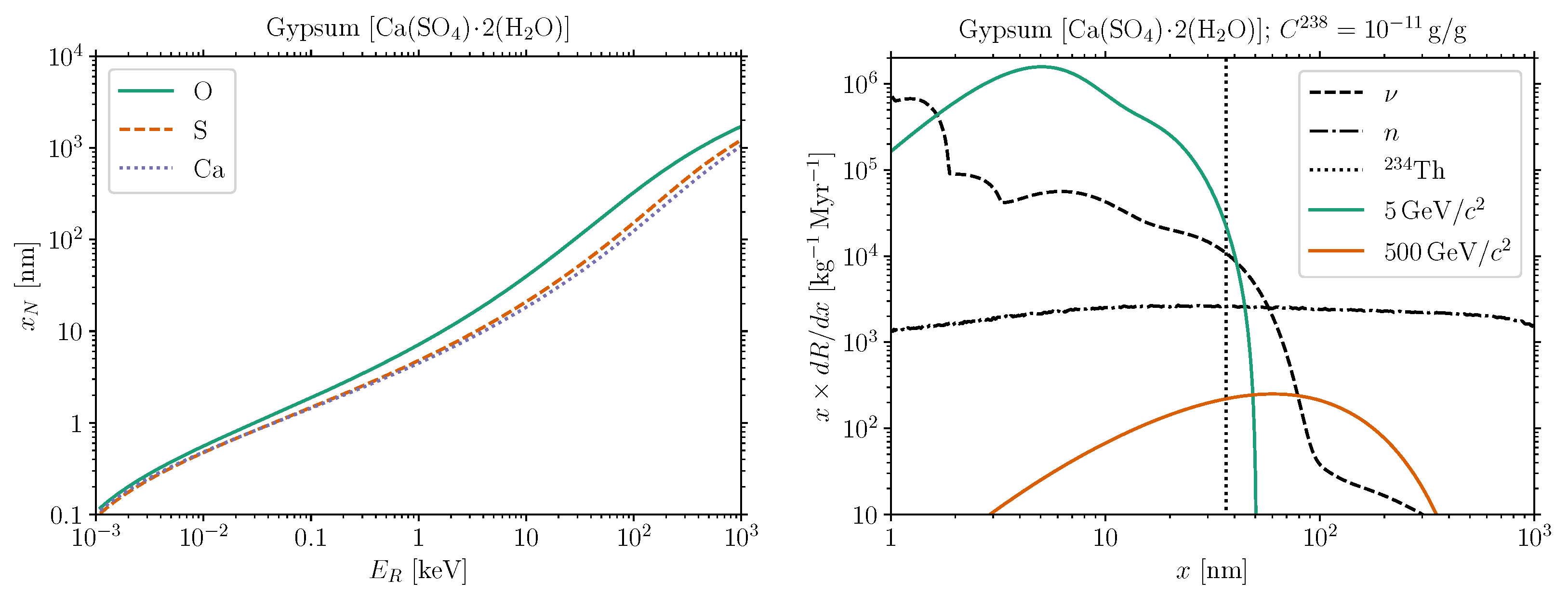
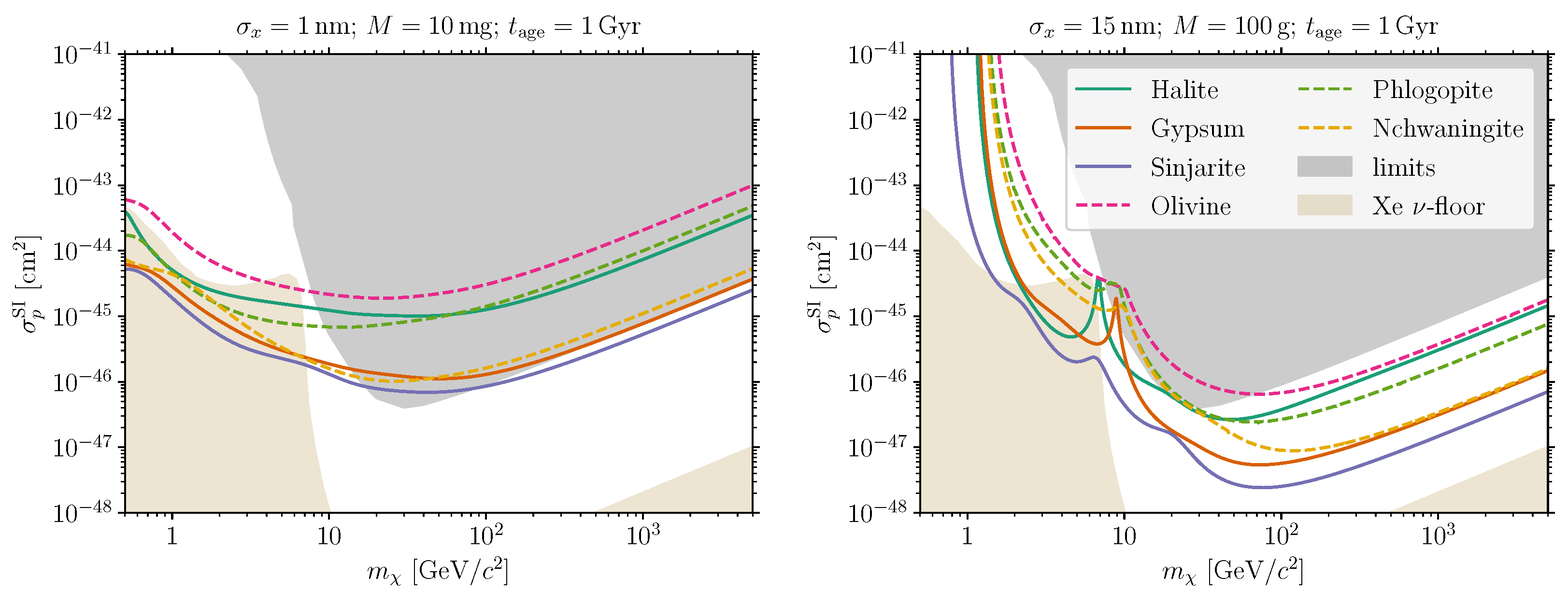
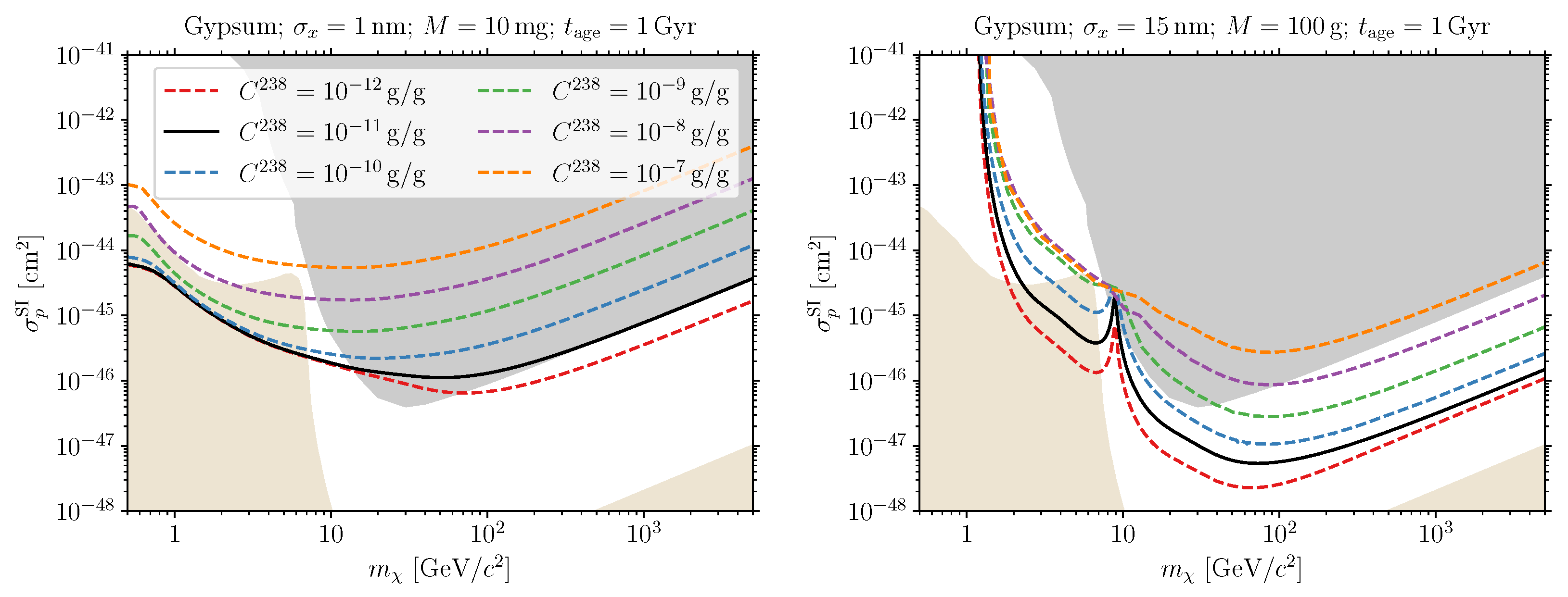
Table 1.
List of minerals considered in this work with their chemical composition and our fiducial assumption for the concentration () in radiopure samples of these minerals.
Table 1.
List of minerals considered in this work with their chemical composition and our fiducial assumption for the concentration () in radiopure samples of these minerals.
| Mineral | Composition | Fiducial U Concentration [per Weight, g/g] |
|---|---|---|
| Halite | NaCl | |
| Gypsum | Ca(SO(HO) | |
| Sinjarite | CaClHO) | |
| Olivine | MgFe(SiO) | |
| Phlogopite | KMgAlSiOF(OH) | |
| Nchwaningite | MnSiO(OH)HO) |
Publisher’s Note: MDPI stays neutral with regard to jurisdictional claims in published maps and institutional affiliations. |
© 2021 by the authors. Licensee MDPI, Basel, Switzerland. This article is an open access article distributed under the terms and conditions of the Creative Commons Attribution (CC BY) license (https://creativecommons.org/licenses/by/4.0/).
Share and Cite
MDPI and ACS Style
Baum, S.; Edwards, T. .; Freese, K.; Stengel, P. New Projections for Dark Matter Searches with Paleo-Detectors. Instruments 2021, 5, 21. https://0-doi-org.brum.beds.ac.uk/10.3390/instruments5020021
AMA Style
Baum S, Edwards T , Freese K, Stengel P. New Projections for Dark Matter Searches with Paleo-Detectors. Instruments. 2021; 5(2):21. https://0-doi-org.brum.beds.ac.uk/10.3390/instruments5020021
Chicago/Turabian StyleBaum, Sebastian, Thomas D. P. Edwards, Katherine Freese, and Patrick Stengel. 2021. "New Projections for Dark Matter Searches with Paleo-Detectors" Instruments 5, no. 2: 21. https://0-doi-org.brum.beds.ac.uk/10.3390/instruments5020021