Short-Term Forecasting Photovoltaic Solar Power for Home Energy Management Systems


1
Faculdade de Ciência e Tecnologia, Universidade do Algarve, 8005-294 Faro, Portugal
2
IDMEC, Instituto Superior Técnico, Universidade de Lisboa, 1049-001 Lisboa, Portugal
3
CISUC, University of Coimbra, 3030-290 Coimbra, Portugal
*
Author to whom correspondence should be addressed.
Inventions 2021, 6(1), 12; https://0-doi-org.brum.beds.ac.uk/10.3390/inventions6010012
Submission received: 21 December 2020
/
Revised: 10 January 2021
/
Accepted: 22 January 2021
/
Published: 25 January 2021
(This article belongs to the Special Issue Photovoltaic Array Management)
Abstract
:Accurate photovoltaic (PV) power forecasting is crucial to achieving massive PV integration in several areas, which is needed to successfully reduce or eliminate carbon dioxide from energy sources. This paper deals with short-term multi-step PV power forecasts used in model-based predictive control for home energy management systems. By employing radial basis function (RBFs) artificial neural networks (ANN), designed using a multi-objective genetic algorithm (MOGA) with data selected by an approximate convex-hull algorithm, it is shown that excellent forecasting results can be obtained. Two case studies are used: a special house located in the USA, and the other a typical residential house situated in the south of Portugal. In the latter case, one-step-ahead values for unscaled root mean square error (RMSE), mean relative error (MRE), normalized mean average error (NMAE), mean absolute percentage error (MAPE) and R2 of 0.16, 1.27%, 1.22%, 8% and 0.94 were obtained, respectively. These results compare very favorably with existing alternatives found in the literature.
1. Introduction
Photovoltaic (PV) power generation has achieved enormous development in recent years, mainly for becoming a significant component of the modern power industry’s decarbonization. Considering PV power generation in buildings, the PV panels are strongly evolving from off-grid systems to grid-connected systems associated with smart energy management systems (EMS) solutions. The PV power output depends on the available solar irradiation incident on the panels, and this value is not uniform over time. A part of the fluctuations is deterministic, due to location of the panels and rotational and translational movements of the planet in relation with the sun, being this part correctly described by physical equations [1], as may be found in [2]. However, another part of the fluctuations in solar irradiation availability is due to the presence of clouds, cloud mass, aerosol particle concentration, wind speed and direction, ambient temperature, among others, which stochastically reduce the PV panel power output [3,4]. Moreover, the PV panels’ output power depends also on internal factors, as photovoltaic module temperature affects the radiation power conversion efficiency [3].
These unpredictable factors generate uncertainty associated with its forecasting to the power grid and to the implementation of the EMS that is dependent on the forecasting of PV power output. In this sense, PV power output accurate forecasting is a crucial challenge to be overcome to achieve massive PV integration, encouraging the development of many studies at a global level [1].
Scope of the Work, Objective, and Organization
The present work is included in a larger research project, non-invasive load monitoring for intelligent home energy management (NILMforIHEM). The main objective of this project is to improve the performance of home energy management systems (HEMS) using improved non-invasive load monitoring methods (NILM), model-based predictive control (MBPC) algorithms employing improved forecasting algorithms, and state of the art heating, ventilation and air conditioning (HVAC) control systems. Different forecasting models are used for MBPC HEMS, namely PV power generation, house consumption—which can be subdivided into schedulable and non-schedulable appliances—weather, and home thermal comfort.
This work is focused on the first type of models, PV electric power generation. As the forecasts will be used for MBPC of the inverter, multi-step forecasting models should be designed, meaning that, at every instant k, forecasts of the PV power for instants k + 1, k + 2, …, k + PH should be obtained, being PH the prediction horizon. A compromise should be established between the step size used (time-difference between the samples) and the PH employed. A 15-min time-step is typically employed in the technical requirements for interchanging energy information between prosumers and the energy suppliers, the reason to consider it as the step size. A good compromise for the prediction horizon would be 12 h due to computational load, resulting in 48-steps-ahead forecasting (being the 15-min interval between steps of the prediction horizon).
Assuming these settings, this work’s main goal is to improve PV power forecasting accuracy by employing existing methods. Additionally, envisioning possible commercial use, these forecasting models should utilize only a few months of data, in contrast with other studies that use more prolonged periods of design data as, for example [5]. The amount of data available improves the predictions’ reliability; however, extensive databases are not available for new buildings that would benefit from using a HEMS such as the one described.
The manuscript is organized into five sections. Section 1 presents the introduction to the topic and the scope of the work. Section 2 presents a brief literature review covering forecasting approaches based on computational learning for solar irradiation and PV power. Metrics used for comparability of studies and results obtained by previous studies, are also shown. Section 3 presents the methodology proposed in this work, focusing on the data selection method, and the model design framework. Section 4 presents two case studies, the first using data from a specially built house in the USA, and the second based on a typical residence in Portugal’s Algarve region. The first case study is used to determine the inputs employed for the forecasting models and their structure. Section 5 compares the results obtained with the Algarve residence with the ones obtained in previous approaches, selected in Section 2. Finally, conclusions and guidelines for future work are drawn in Section 6.
2. Literature Review
This section briefly reviews PV power forecasting approaches based on computational intelligence applied to model-based predictive control (MBPC) and scheduling energy management applications. Performance metrics and results of pertinent studies that may be an object of comparison are also highlighted.
Like airlines, consumer package goods, and oil and gas industries, the electric power industry needs forecasts of supply, demand and price, the so-called energy forecasts, to plan and operate the grid. As electricity cannot be massively stored using today’s technologies, electricity must be generated and delivered as soon as it is consumed. In other words, utilities must balance the supply and demand at every moment.
The type of solar resource to be forecast depends on the installed technology. For concentrating photovoltaics (CPV), direct normal incident irradiance (DNI) must be forecasted. Because of non-linear dependence of concentrating solar-thermal efficiency on DNI and the controllability of power generation through thermal energy storage (if available), DNI forecasts are especially crucial for the management and operation of CPV power plants. DNI is impacted by phenomena that are very difficult to forecast, such as cirrus clouds, wildfires, dust storms, and episodic air pollution events, reducing DNI by up to 30% on otherwise cloud-free days. For non-concentrating systems (i.e., most PV systems), primarily global irradiance (GI = diffuse + direct) on a tilted surface is required, which is less sensitive to errors than DNI since a reduction in clear-sky DNI usually increases diffuse irradiance. For higher accuracy, forecasts of PV-panel temperature are needed to account for the (weak) dependence of solar-conversion efficiency on PV-panel temperature [6]. This section does not aim to describe the physics behind solar energy PV power generation, as they are well known and widely available sources in the literature. The interested reader can find details in [7,8,9].
Forecasting models for solar irradiance can be broadly classified as [10]: statistical, cloud-based, and numerical weather prediction (NWP) models.
Statistical models can be further subdivided into linear models (persistent forecasts, using the clearness or clear sky indexes, or Fourier series expansions, AutoRegressive–Moving-Average—ARMA, AutoRegressive Integrated Moving Average—ARIMA or Classification And Regression Trees—CART models) and non-linear, typically computational intelligence-based models (neural networks, wavelet, fuzzy or evolutionary). Cloud-based models use weather satellite images or ground-based sky (GBS) images [11] to improve solar irradiance forecast. Basically, by processing previous sky images, clouds can be detected, and their motion extrapolated using motion vector fields, or sky cover indices can be obtained, and their evolution forecasted. GBS images have been shown to improve statistical models’ performance for forecasts up to 6 h in advance. NWP models are used to forecast the state of the atmosphere up to 15 days ahead. The main limitation of NWP forecasting is its coarse resolution. Spatial resolution can be as low as 1 Km, but the minimum temporal resolution is typically 3 h, which does not allow its use for any patterns less than this value.
The choice of solar-forecasting method depends strongly on the timescales involved, which can vary from horizons of a few seconds or minutes (intra-hour or very short forecasts, for control and adjustment actions), a few hours (intra-day or short/medium, for energy resource planning and scheduling as well as for the electricity market), to a few days ahead (intra-week or long, for unit commitment and maintenance schedules) [12]. The ability to forecast solar irradiance in near-real-time, or nowcasting, is crucial for network operators to guarantee power grid stability with specific reference to power plant operations, grid balancing, real-time unit dispatching, automatic generation control and trading, and for home energy management systems. As this work aims to incorporate the PV power forecasts in HEMS, the authors are interested in real-time, intra-hour and intra-day forecasts.
The accuracy of solar radiation forecasting has direct financial impacts, at various levels. For example, in [13] the effect of DNI forecast accuracy on concentration solar thermal (CST) plants’ financial value, incorporating energy storage is examined. When the RMSE of a 48-h DNI forecast is between 325 and 400 W/m2, a 1 W/m2 improvement increases the financial value by $400–1300 per six months’ operation for a CST plant. Excellent reviews of solar irradiance forecasting are available, such as [10,14,15,16,17,18].
Focusing now on PV power generation forecasting, it is, in a simplistic definition, the application of techniques that use registered historical data to make informed prediction/estimation of the future value that PV power will assume in a defined prediction horizon. These forecasts can be obtained directly, i.e., a model is developed using inputs lags of the endogenous variable and, possibly, exogenous ones. Alternatively, forecasting models of those exogenous variables are designed first, and their outputs are fed to a static model which generates the forecasts of the PV power. In [19], the correlations between PV power output and several input variables are explained and computed, concluding that the solar irradiance’s correlation achieves large values such as 0.988, followed by the panel temperature and the ambient temperature.
The same categories of models pointed out for solar irradiance forecasting apply to PV generation forecasting [12,20,21,22,23].
Throughout the years, the use of computational intelligence models for forecasting applications has been steadily increasing and, this way, are the focus of this synthetic survey presented in the next sub-section. Computational learning is a mathematical and theoretical field of artificial intelligence that analyses machine learning algorithms’ design and their learnability capacity while improving the necessary functions’ accuracy and efficiency. These models are based on estimating a function deduced only from samples of training data describing a specific system’s behavior and are well suited when physical features are not known [20]. As these are data-based models, the lack of accurate data can become an issue for computational learning methods [20], as the accuracy is strongly dependent on the quality and amount of the available data.
The most used computational learning architectures used for PV power forecasting are shallow and deep artificial neural networks, support vector machine and fuzzy models.
For solar power forecasting, ANNs are among the most employed machine learning techniques. Artificial neural networks are inspired in the biologic neuron and networks. A neural network’s fundamental processing element is a neuron, which performs a simple computation on its inputs. Neurons are typically grouped into layers. The network usually consists of an input layer, some hidden layers, and an output layer. ANNs can somehow be classified by the neuron model employed, number of layers, neurons interconnection and the training mechanism. The forecasting performance of an ANN model depends not only on the above items, but also on the design data, and the inputs employed.
The ANN model used in this work is a radial basis function (RBF) Neural Network (NN). The hidden neurons employ a radial type of function, typically a Gaussian, their outputs being linear combined afterwards. Thus, the output of an RBF model is given by:
In (1), y[k] denotes the output, at instant k, i[k] is the jth input at that instant, w represents the vector of linear weights, C(j) represents the vector (extracted from the C matrix) of the centers associated with hidden neuron j, σj is its spread, and ||2 denotes the Euclidean distance. RBFs, as well as multilayers perceptrons (MLP), B-spline neural networks and others, are nowadays called shallow ANNs [24], in contrast with deep architectures, employing a larger number of layers, such as deep neural networks, deep belief networks, long-short term memory neural networks (LTSM) and convolutional neural networks (CNN).
Yang and co-workers [25] proposed a hybrid scheme, involving classification, training, and forecasting stages. In the classification stage, self-organizing maps and learning vector quantization networks classify the collected historical data of PV power output. The training stage employed the support vector regression to train the input/output data sets for temperature, probability of precipitation, and solar irradiance of defined similar hours. In the forecasting stage, the fuzzy inference method was used to select an adequately trained model for an accurate forecast. This scheme is used for one-day ahead hourly forecasting of PV output.
Leva and co-workers [12] used an MLP to forecast the hourly day-ahead PV power, based on weather forecasts, and power and irradiance measurements. Having available a 72-h weather forecast, in each day x an hourly forecast for day x + 1 was produced, between sunrise and sunset.
In [26], a 72 h deterministic and probabilistic forecast of PV power output was developed using MLPs combined with an analog ensemble, using as inputs forecasts of global irradiance, cloud cover and atmospheric temperature, obtained from a numerical weather prediction model, as well as solar azimuth and elevation. Values of RMSE/C (C is the rated power of the PV system) in the range of 8 to 8.7% were obtained.
Rana and co-workers [27] provided twelve different forecasts, from 5 to 60 min ahead, obtained with 12 different prediction models. The authors employed MLPs, arranged in different ways: using single and ensemble models, and using only the past PV power measured values (univariate) and combined with solar irradiance, atmospheric temperature and relative humidly, and wind speed (multivariate). A correlation-based feature selection algorithm was employed for each model, to select the inputs from a set of lags until one-week before, i.e., 12 × 24 × 7 = 840 lags for a univariate model, and 5 × 840 = 4200 lags for multivariate models. In [28], PV power was forecasted for a solar power plant located at the Applied Science Private University, in Jordan. One day-ahead PH was considered, using the measured irradiance values of the five previous days, obtained at the same hour. Employing MLPs, R-squared values for the training, testing and validation sets of 0.97 were achieved.
Addressing now deep architectures, in [29] one day-ahead forecasting was obtained using generative adversarial networks and convolution neural networks to classify weather types, and with trained forecasting PV power models for each type of weather. Unfortunately, no information about the quality of the forecasts was supplied. Zhou et al. [30] employed two long-short-term memory neural networks for PV power output forecasting and atmospheric air temperature, obtaining forecasts for PHs from 7.5 min up to 1 h, using 7.5 min sampling intervals.
Wang and co-workers [31], developed three forecasting models: convolutional neural network, long-short-term memory neural network and an hybrid model (combining the other two models). They used the PV power output itself, the atmospheric air temperature, and the global solar irradiance. MAPE values varying from 2.2 to 11.2% were obtained for a one-step-ahead (5 min) prediction.
Li and co-workers [32] propose a hybrid deep learning approach based on CNN and LSTM for PV output power forecasting. The CNN model is intended to discover the non-linear features and invariant structures exhibited in the previous output power data, thereby facilitating PV power prediction. The LSTM is used to model the temporal changes in the latest PV data and predict the next time step’s PV power. Then, the prediction results in the two models are comprehensively considered to obtain the expected output power.
Hossain and Mahmood [33] employ an LSTM neural network, using as exogeneous variable a synthetic weather forecast. A synthetic weather forecast is created for the targeted PV plant location by integrating the statistical knowledge of historical solar irradiance data with the publicly available sky forecast of the host city. They compared their proposal with recurrent neural networks, generalized regression neural networks and extreme learning machines, for different intraday horizon lengths in different seasons.
The primary purpose of improving the accuracy of solar power forecasts is to reduce the uncertainties related to this type of intermittent energy source, resulting in safer and easier energy management. As solar penetration increases in the energy portfolio, the impact of incorrect forecasts in the grid and HEMS can be larger [1].
A particular model’s performance and accuracy can be assessed via several metrics, which allow the comparison between different models and locations. Each one focus on a certain aspect of point distribution. Thus, there is no unique metric valid for all situations; instead, each one adds some information about the model’s accuracy. In the bibliography, several metrics can be found [34], although there is a group that is more commonly used, such as mean absolute error (MAE) (2), mean relative error (MRE) (3), normalized MAE (NMAE) (4), mean absolute percentage error (MAPE) (5), root mean square error (RMSE) (6) and coefficient of determination (R2) (7). For this reason, these performance criteria will be used in this work, in Case Study 2.
In the previous equations, n is the number of samples, yt is the measured tth value, is the predicted value, C is the rated power of the PV system, and r is the range of the measured variable.
Independently of the metrics used to assess the proposed models’ performance, some other factors hamper comparisons among studies. According to [1], they are climatic variability, day/night values and normalization, sample aggregation, testing period, and specific system attributes. Table 1 presents the summary of pertinent comparable studies in terms of the method used, the prediction horizon, sampling time, input variables, and the model’s accuracy.
Although the works described above are general techniques for short-time and intra-day PV power forecasting, the majority cannot be applied for model-based predictive control and HEMS scheduling. The reason is that MBPC uses predictive models, that should output the modelled variable’s forecasts for each step-ahead within the PH considered, i.e., provide multi-step-ahead forecasting. This type of forecasts can be achieved in a direct mode, by having several one-step-ahead forecasting models, each providing the prediction of each-step ahead within PH. This is the approach followed in [27,32]. An alternative, which is the one followed in this work, is to use a recursive version. In this case, only one model is necessary, and for each step within the PH, the inputs change, eventually employing predictions obtained in previous steps. This way, the RBFs models described in (1) are used as NAR (nonlinear autoregressive) models or NAR models with eXogenous inputs (NARX). Denoting as y the modelled variable, and considering only one exogenous input, v, for the sake of simplicity, the estimation (), at instant k, can be given as (8):
In (8), f(.) represents the RBF model (1), which means that its arguments (the delays of y and v) represent the network input vector, i[k]. As the objective is to determine the evolution of the forecasts over a prediction horizon, (8) is iterated over that horizon. For k + 1, we shall have:
Depending on the indices of the delays, and the steps within the prediction horizon, no measured values may exist for one or more terms in the argument (8). These must be obtained using previous predictions. This way, the computation of the predictions over a prediction horizon PH may require PH executions of the model (8).
Please note that, if multi-step-ahead forecasting is considered (as is the case of this work), the metrics (2–7) can be computed for each step within the prediction horizon. Longer PHs tend to increase forecasting errors, especially under abnormal weather conditions [6], and with an increased interval between samples and with an increasing number of steps. This is more problematic for recursive multi-steps-ahead forecasting methods, as the errors propagate through the steps.
3. Methodology
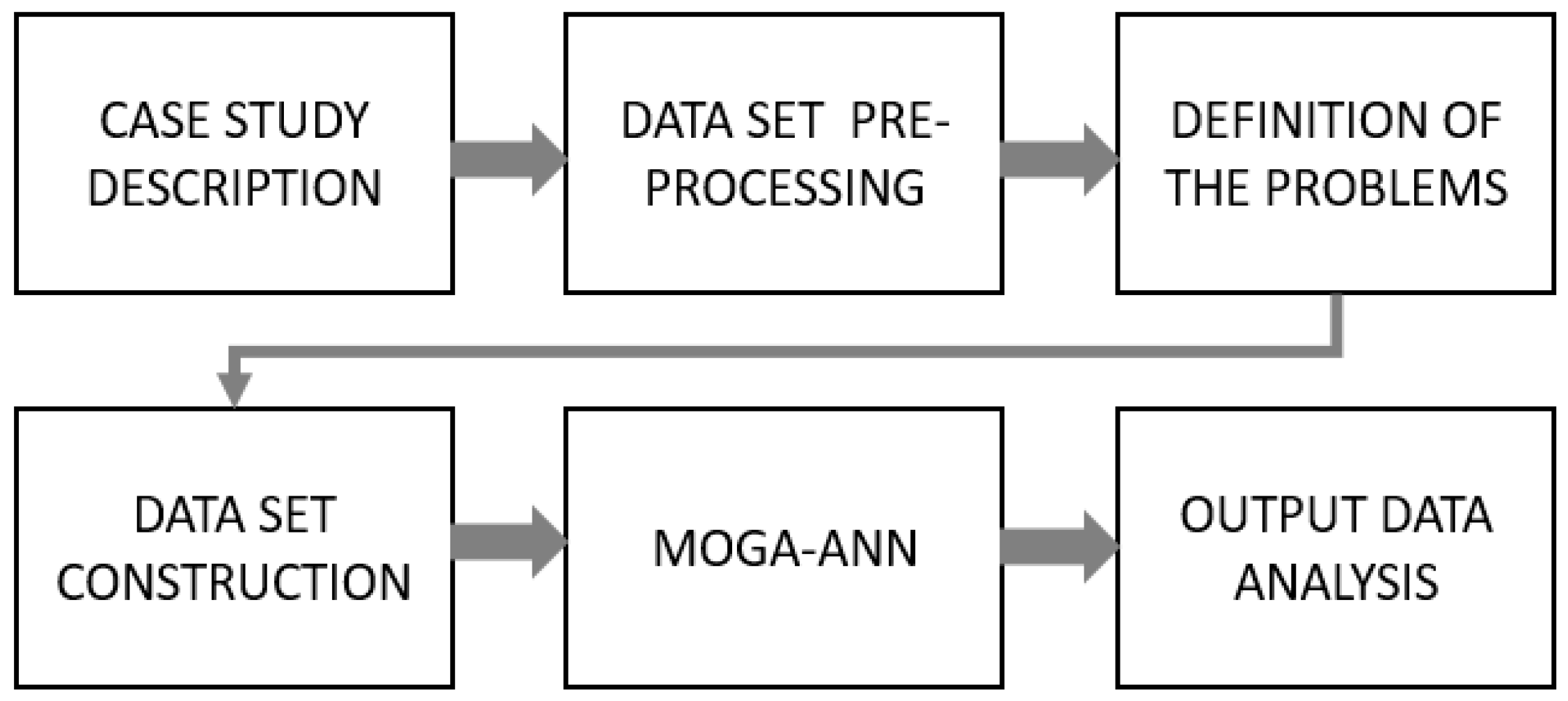
The work methodology employed is divided into six parts (shown in Figure 1), which are used for each case study. The first is the case study description, defined in terms of location and weather, building and PV system characteristics and data acquisition system. The second part is constituted by the data set pre-processing to treat outliers and abnormal data and averaging the acquired data to the employed sampling intervals. The third part is the definition of the model minimization objectives, or constraints when appropriate, and variables and lags definition. The data pre-processing output is then used as input for a data selection algorithm, the ApproxHull, described below. The fifth part is the design of one model, or an ensemble of models, involving input selection, topology determination (number of neurons) and parameters estimation. The MOGA framework achieves the model design (please see Section 3.2). The analysis of the forecasts obtained constitutes the sixth part. The fourth and fifth steps are briefly reviewed in the next sub-sections.
The case studies are described in Section 4 (please see Section 4.1 and Section 4.2). In summary, two case studies were used to develop this work concerning the short-term forecasting. The first is composed by the dataset of the Honda Smart Home US, developed by Honda, which makes the data publicly available each six months. The input data used for the first case study are the PV power output, ambient air temperature, PV panel temperature and solar irradiance. The detailed data from Case Study 1 may be found in its website, as referenced in Section 4.1, as well as many other variables measured in that household. The second case study is composed by the dataset of a typical Portuguese household, located in Algarve, Portugal. This house is the main case study of the project NILMforIHEM where this work is inserted, and has an extensive acquisition system monitoring different variables related to the energy consumption of the building. Case study 2 uses as input data the PV power consumption, the ambient air temperature and the solar irradiation. At the time of publication, the access to the data is only available to the research group.
3.1. Data Set Construction
This work uses the ApproxHull algorithm proposed in [35], to select data for training, testing and validation data for the artificial neural networks design. ApproxHull is an incremental randomized approximate convex hull (CH) algorithm that selects the points involving whole data points. It is applicable to high dimension data, treating memory and time complexity efficiently. The convex hull vertices obtained are compulsorily introduced in the training set so that the model can be designed with data covering the whole operational range.
A pre-processing phase is performed on the original data set before applying the convex hull, normalizing the dimensions in the range of (–1, 1). Very briefly, it starts with an initial convex hull (the maximum and minimum of each dimension), and subsequently, the current convex hull grows by adding the new vertices into it. Then, it generates a population of k facets based on the existing convex hull, selecting the furthest points in the current facets’ population as new vertices of the convex hull, which are integrated into the current convex hull. A detailed explanation of the convex hull algorithm may be found in [35].
3.2. MOGA Design
The model design problem is typically considered as multi-objective optimization, with possible restrictions and priorities. The MOGA design framework is a hybrid of an evolutionary algorithm and a derivative-based algorithm. The evolutionary part searches the number of neurons’ admissible space and the number of inputs (lags for the modelled and exogenous variables) for the RBF models. For this reason, the structure of the chromosome includes the number of neurons and pointers for the admissible delays of the endogenous and exogeneous variable(s), if available. Details on the MOGA method were previously published in [35]. Before being evaluated in MOGA, each model has its parameters determined by a Levenberg–Marquardt (LM) algorithm [36,37] minimizing an error criterion that exploits the linear-nonlinear relationship of the RBF NN model parameters [38,39]. Basically, denoting by X the input matrix, and by v and w the vectors of nonlinear parameters (C and σ) and linear output weights, respectively, the model output vector, y, can be given as:
Denoting by t and e the target and error vector, the training criterion usually employed is:
Independently of the value of the nonlinear parameters, the optimal value of the linear parameters can be obtained as the least squares solution:
If this value is incorporated in (11), a new criterion (independent of the linear parameters) is obtained:
Any derivative algorithm can be employed to minimize (13). In our case, the LM method is used. The initial values of the non-linear parameters are chosen randomly, or with the use of a clustering algorithm, w is determined as a linear least-squares solution, and the procedure is usually terminated using the early-stopping approach within a maximum number of iterations.
The framework requires the data used to develop the models to be divided into three data sets: a training set, used to estimate the model parameters, a testing set, for terminating the training, and a validation set, for comparing the performance of the models obtained by executing MOGA (as it uses a multiple objective formulation, its results are not a single solution, but a set of non-dominated solutions). The minimization objectives used in this work are the RMSEs of the training set and the testing set, the model complexity (O(µ)) and the forecasting error (εp). This last criterion is obtained by summing the RMSEs along with PH (14), where D is a time-series, with p data points, and E is an error matrix (15):
In this work, MOGA is executed with 100 generations, population size of 100, the proportion of random emigrants of 0.10 and a crossover rate of 0.70. The admissible range of neurons varied from 2 to 20, while the admissible number of inputs considered ranged from 2 to 20. After execution, the selection of one model from the non-dominated or Pareto solutions is then performed based on the objective values obtained, the RMSE obtained over the validation data set, and the prediction performance (15) over a user-specified period, which may coincide with D.
Typically, two executions of MOGA are performed. By analyzing the results of the first execution the search space can be reduced, by shortening the admissible range of inputs and/or the number of neurons, and/or set restrictions for some objectives, and assigning different priorities. Examples of MOGA application for various applications can be seen in, for instance, [40,41,42,43].
As mentioned above, the output of MOGA is not a single solution, but a set of non-dominated models (or preferable models, if restrictions are used). A best model can be selected to represent the results obtained by the problem. However, the non-dominated (or preferable) set of models can also be employed for ensemble averaging the outputs of these models. As the forecasting criterion (15) is not used as a MOGA restriction, models can deliver a very bad prediction performance in a few situations and should be considered outliers among the non-dominated set. This can be solved if the median of the results obtained in the dominant (or the preferable) set, and not their mean value, is used as the ensemble’s output. For an example of applying the ensemble approach for forecasting electricity consumption, please see [44].
4. Case Studies and Results
4.1. Honda Smart Home US
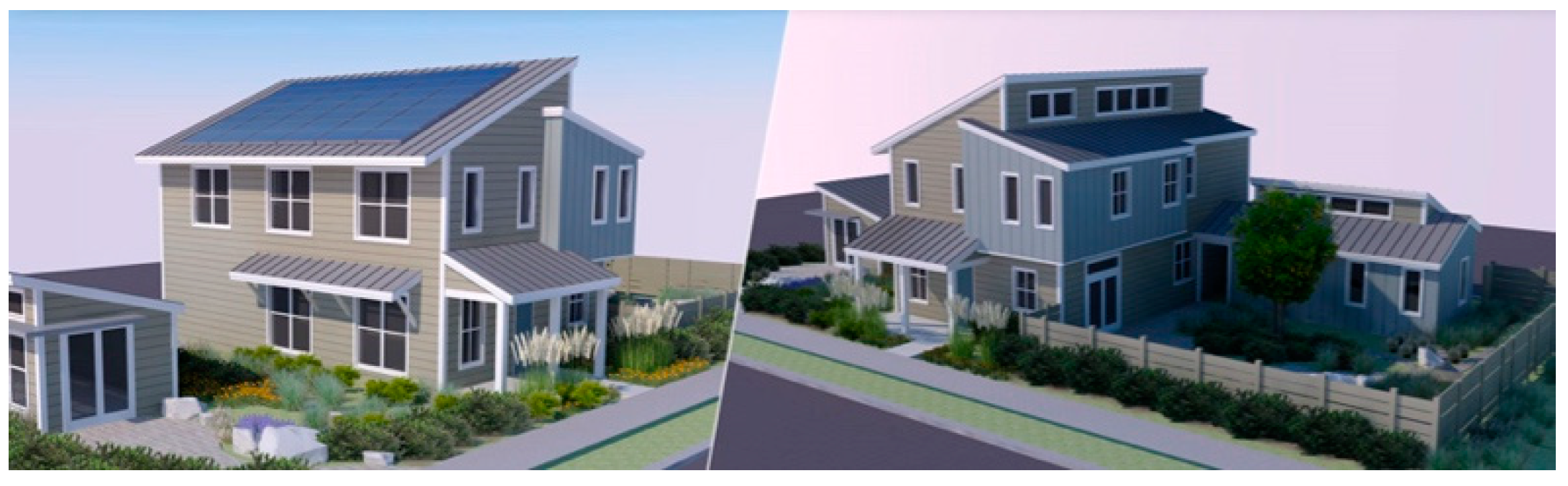
The first case study uses data obtained in the Honda Smart Home (HSH) US [45] (Figure 2). This net zero energy building is located on the West Village campus of the University of California, Davis. It used sustainable construction materials, has a radiant floor night ventilation and a photovoltaic system. Electric appliances and lighting have high efficiency, and the HVAC system employs a ground-source heat pump. The household has a complex home energy management system to control the electric systems. Details about the construction, electric appliances and data acquisition system details can be found on its website [45].
The group responsible for the HSH makes available experimental data every six months. Based on the publicly available data, studies were developed, focused mainly on the integration between electric vehicles and the smart home, the home management systems of the HVAC solutions, and construction practices. The present work uses the HSH data for a first design of the forecasting PV power model. In the first step, the exogenous variables to be employed will be selected, and subsequently, the structure of the model will be defined.
To develop the present study, four variables are used from the HSM data set. They are the global solar irradiance, the PV panels’ temperature, atmospheric air temperature, and PV DC power produced. Data from 1st January 2016 to 31st December 2018 has been acquired with a sampling time of 1 min and averaged by the authors in 15 min. Not all data was valid for the four variables simultaneously, whether because of lack of data, or wrong measurements. After cleaning, from the 105,217 available samples, 81,504 values were available for model design.
Within the data considered, the air temperature ranged from −1.6 to 42.8 °C, the panel temperature from −6.5 to 84.6 °C, the maximum of solar irradiance was 1127 W/m2, and of the PV power 9.3 kW.
4.1.1. PV Power Static Mappings
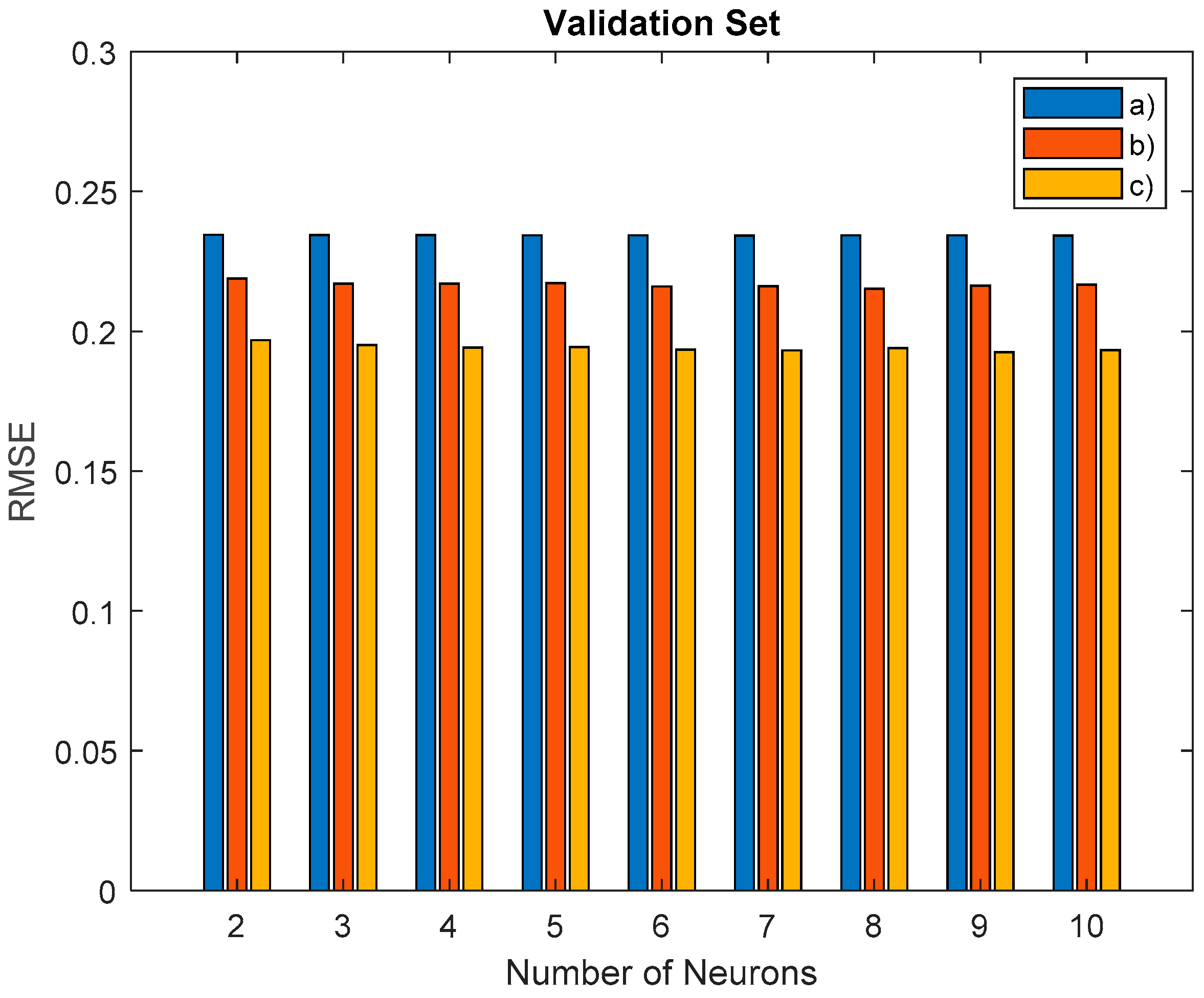
The first set of experiments was conducted to determine if the PV power was better approximated by the solar irradiance alone (a), combined with the air temperature (b) or with the PV panel temperature (c). Notice that this a simple static mapping and no forecasting is obtained or desired.
As this is a simple problem, MOGA was not employed. Using only the samples with non-null PV power, the 81,504 values were reduced to 50,525 samples. ApproxHull was employed, resulting in 29,008, 9669 and 9671 samples for training, testing and validation. For each input configuration, models were designed where the number of hidden neurons ranged from 2 to 10. For each configuration pair (inputs and number of neurons), five different trainings were performed using a modified version of the Levenberg-Marquardt algorithm [46], with different initial values of the RBF centers determined using an optimal adaptive k-means algorithm [47]. Each training was terminated using the testing dataset for early-stopping. The model that achieved the best compromise between the RMSEs of the training and test sets and the linear parameters norm was selected for the corresponding configuration pair.
Figure 3 illustrates the RMSEs obtained in the validation set for the three different model configurations (a, b and c), with neurons ranging from 2 to 10. As can be seen, the models using only solar irradiance as input obtain the worst results, while the models using solar irradiance and panel temperature as inputs achieve the best performance. A compromise solution is to employ solar irradiance and air temperature, as it is more widely available than the panels’ temperatures.
4.1.2. PV Power Dynamic Model
Considering the previous results, the exogenous inputs for PV power forecasting will be the solar irradiance and the atmospheric air temperature. As expressed before, recursive multi-step ahead forecasting models will be used. There are, however, two ways of obtaining the forecasts of the PV power: whether we design two forecasting models of the two exogenous variables and pass those values through a static PV model, or we use a single model, which outputs the PV power forecasts. The two approaches were considered, but the latter obtained the best results. Because of that, it will be discussed here.
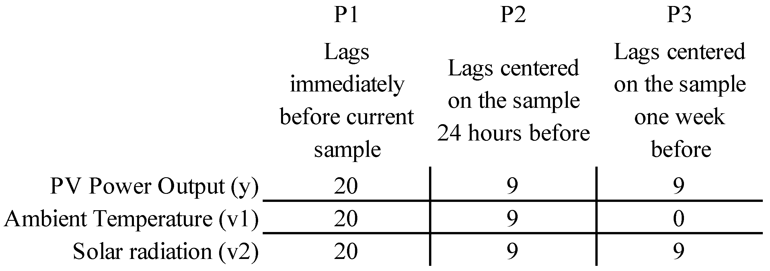
Samples corresponding to three different periods: P1—lags immediately before the current sample; P2—lags centered on the sample 24 h before; P3—lags centered on the sample one week before will be employed. Considering that each period has three values, the first for PV power, the second for air temperature and the third for solar irradiation, the lags employed are presented in Figure 4. This means that each design sample (out of the 81,504 available) consists of 105 lags (38 for PV power, 29 for air temperature and 38 for solar irradiation. As the largest lag corresponds to 676, and a PH of 48 (12 h) is desired, 676 + 48 = 724 samples cannot be employed, resulting in 80,780 samples available for model design
Using this data, ApproxHull found 1512 convex-hull points, mandatorily incorporated in the training set. The number of samples for training, testing and validation were 48,468, 16,156 and 16,156 respectively. The prediction set employed two weeks of data, from 3 June 2018, 23:45:00 to 17 June 2018, 23:45:00.
The design problem was formulated as minimizing the RMSE of the training and testing set, the model complexity and the forecasting error (15). MOGA obtained 307 non-dominated models. The minimum values for the errors obtained are shown in Table 2. Please note that scaled values between −1 to +1 are employed here.
A model was chosen obtaining a good compromise between the performance criterion, whose structure is shown below (16).
As can be seen, for the three variables, samples belonging to the three periods considered were selected. Some statistics related to the performance of the selected model (16) are shown in Table 3.
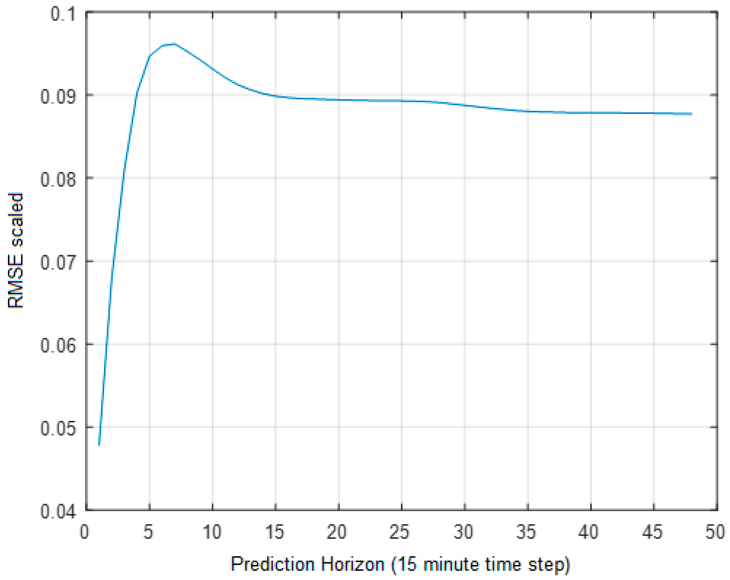
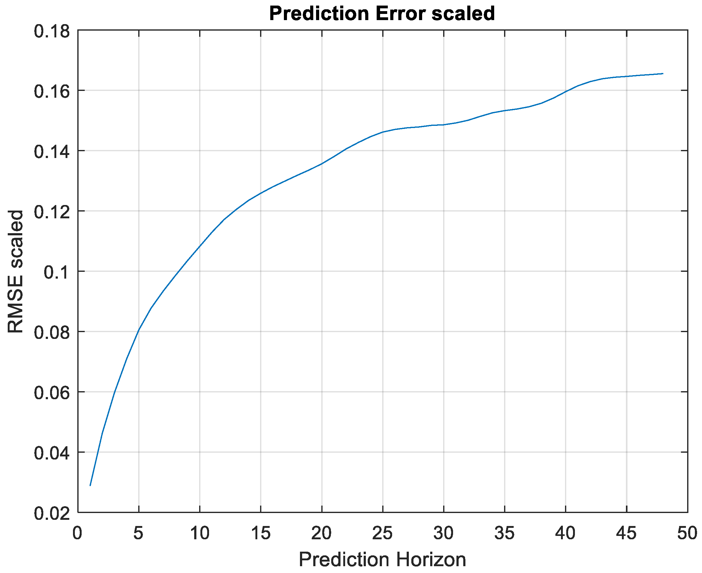
The evolution of the RMSE over the PH, using scaled data, can be seen in Figure 5. Each value in the prediction horizon axis is equivalent to one step of 15 min—and so, 48 steps ahead in the prediction horizon axis is equivalent to 12 h ahead. The same is valid for the similar figures that follow.
Although the errors increase as we are moving up the number of steps-ahead, the prediction error 12 h ahead is just the double of 15 min ahead. This indicates that a larger PH could be considered, if necessary.
4.2. Algarve Residence
The residence of this case study (Figure 6) is in Gambelas, Faro, Algarve, Portugal (37°0′55″ N, 7°56′6″ W). Faro lies 3 m above sea level, and the climate is warm and temperate, with winters rainier than the summers. The climate here is classified as Csa (Hot Summer Mediterranean Climate) by the Köppen–Geiger system [48,49]. The average temperature in this city is 17.2 °C, and precipitation is about 501 mm.
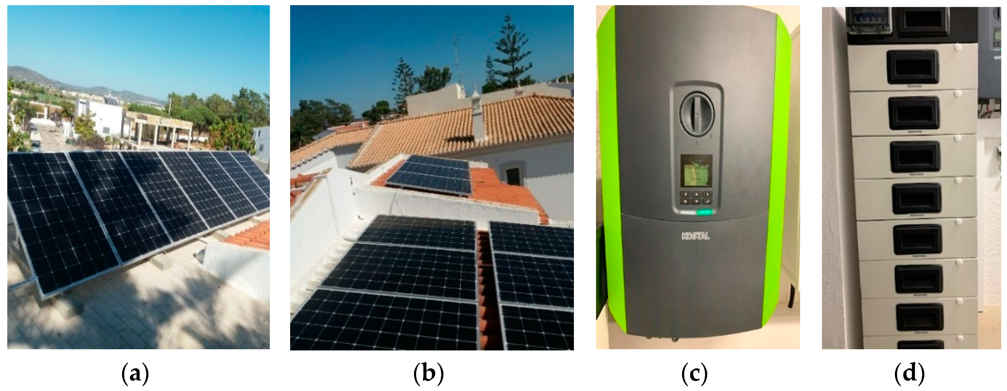
The residence employed is a detached house, with two floors and with 20 different spaces. The household has a PV installation, composed of 20 Sharp NU-AK panels [50], arranged in two strings, each panel with a maximum power of 300 W. The inverter is a Kostal Plenticore Plus converter [51], which also controls a BYD Battery Box HV H11.5 (with a storage capacity of 11.5 kWh) [52]. An intelligent weather station is also installed, which measures solar irradiance and atmospheric air temperature and computes their evolution within a user-specified PH [53]. Many (several hundred) variables are acquired, either with a sampling time of 1 s or 1 min. The data acquisition system is described in the authors’ previous work and may be found in [33].
Only three variables are used for the current work: the PV DC power produced, atmospheric air temperature, and global solar irradiance. Data from 19 May 2020 17:37:30 to 31 July 2020 23:52:30 is used, averaged in 15 min steps. As the same values for the three periods of lags are the same as used for the Honda house, the 7034 samples were reduced to 6310 available for model design. Please note that in this second case study a much smaller number of samples is employed, as, in a practical situation, it is not possible to wait three years of data before designing forecasting models. The maximum values of DC power and solar irradiation are 6 kW and 1177 W/m2, and the air temperature ranged from 11.7 to 38.2 °C.
In contrast with the model developed for the Honda house where, throughout the prediction horizon, measured data was used for the exogeneous variables, here forecasts of these variables, whenever needed, are obtained from corresponding forecast models. This means that forecasting models for solar irradiance and the air temperature must also be designed.
Common to the three models, the prediction set employed nearly one month of data, from 14 June 2020, 00:07:30 to 12 July 2020, 23:52:30. The design problem will also be formulated, as in the Honda house, as minimizing the RMSE of the training and testing set, the model complexity, and the forecasting error (15).
4.2.1. Solar Irradiance Model
This is a NAR model, which means that no exogenous variables are used in the model. Similarly, as in the Honda house, 38 lags from the three different periods were considered, 20 for P1 and 9 for P2 and P3. After duplicate samples have been removed, 5366 samples were available for model design. AproxHull found 909 convex hull vertices, which were incorporated in the training set. The training, testing and validation sets had 3219, 1073 and 1074 samples, respectively.
MOGA produced 451 non-dominated models. The minimum, mean and maximum values of the root-mean-square errors (, , ) for the training, testing and validation sets are shown in Table 4. Please notice that these values are obtained using data scaled between −1 and +1, and that they should be multiplied by 10−1.
The structure of the selected model is shown below (17).
Some statistics related to the performance of the selected model are shown in Table 5.
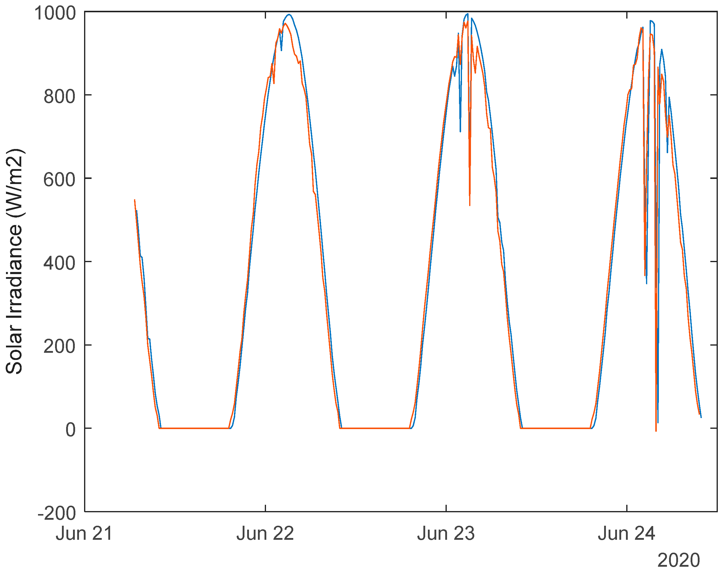
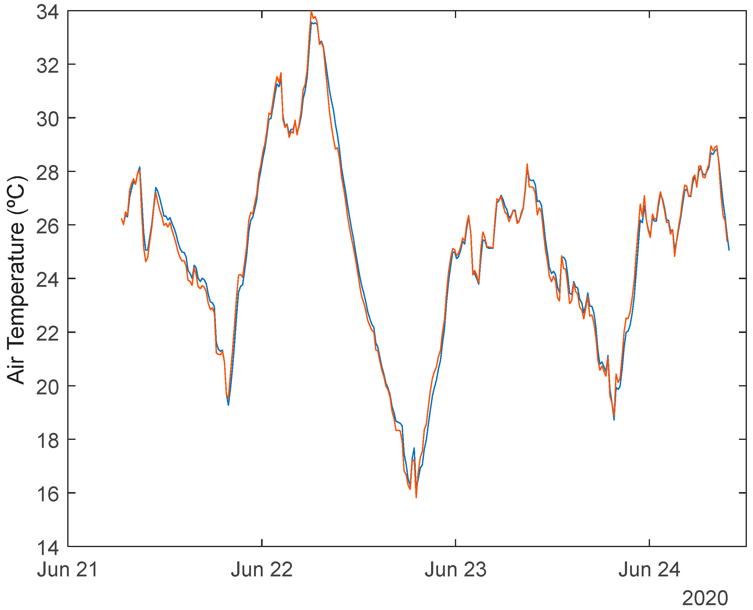
The evolution of the RMSE over the prediction horizon is shown in Figure 7, and the measured and one-step-ahead air temperature are shown in Figure 8, for four selected days. These days (from 21 June to 24 June) were selected due to the good conditions for solar photovoltaic energy generation in terms of solar irradiation exposure (sunny day, as is possible to see in Figure 8—the solar irradiance reaches nearly 1000 W/m2). The ambient air temperature for these days also were representative for the characteristic Algarve sunny days in Spring and Summer seasons.
4.2.2. Air Temperature Model
The same 38 lags were considered for this model. No duplicate samples were found, and therefore 6310 samples were available for model design. AproxHull found 669 convex hull vertices and the training, testing and validation sets had 3786, 1262 and 1262 samples, respectively.
MOGA produced 393 non-dominated models. Statistics of the RMSE for the training, testing and validation sets are shown in Table 6. Please notice that these values should be multiplied by 10−2. As it is possible to see for the three sets, the maximum values are considerably higher than the average values, which represent a slight increase in relation to minimum values, meaning that in the set few results are nearly maximum values.
The structure of the selected model is shown below.
Some statistics related to the performance of the selected model are shown in Table 7. The results for the error parameters are similar in the cases of training, testing and validation. While the first three sets (training, testing and validation) present lower values, the sum of the prediction error is slightly higher than in the previous case (solar irradiance model).
The evolution of the RMSE over the prediction horizon is shown in Figure 9, and the measured and one-step-ahead air temperature are shown in Figure 10. The scaled RMSE presented in Figure 9 varies along the prediction horizon from 0.03 to 0.165, which can be considered a very good result. As is possible to see in Figure 10, the one-step predicted values are very close to the measured values.
4.2.3. PV Power Model
ApproxHull found 1343 convex hull points. The training, testing and validation sets consisted of 3786, 1262 and 1262 samples, respectively. MOGA produced 268 non-dominated models. RMSE statistics for the three sets are shown in Table 8. Please notice that the values should be multiplied by 10−2. The differences between the maximum and minimum values in the non-dominated set are lower for this model, in comparison with the ambient temperature model, and the average values superior.
The structure of the selected model is shown below. In contrast with the one selected for the Honda house, the exogenous variables’ lags only belonged to Period 1.
Some statistics related to the performance of the selected model are shown in Table 9.
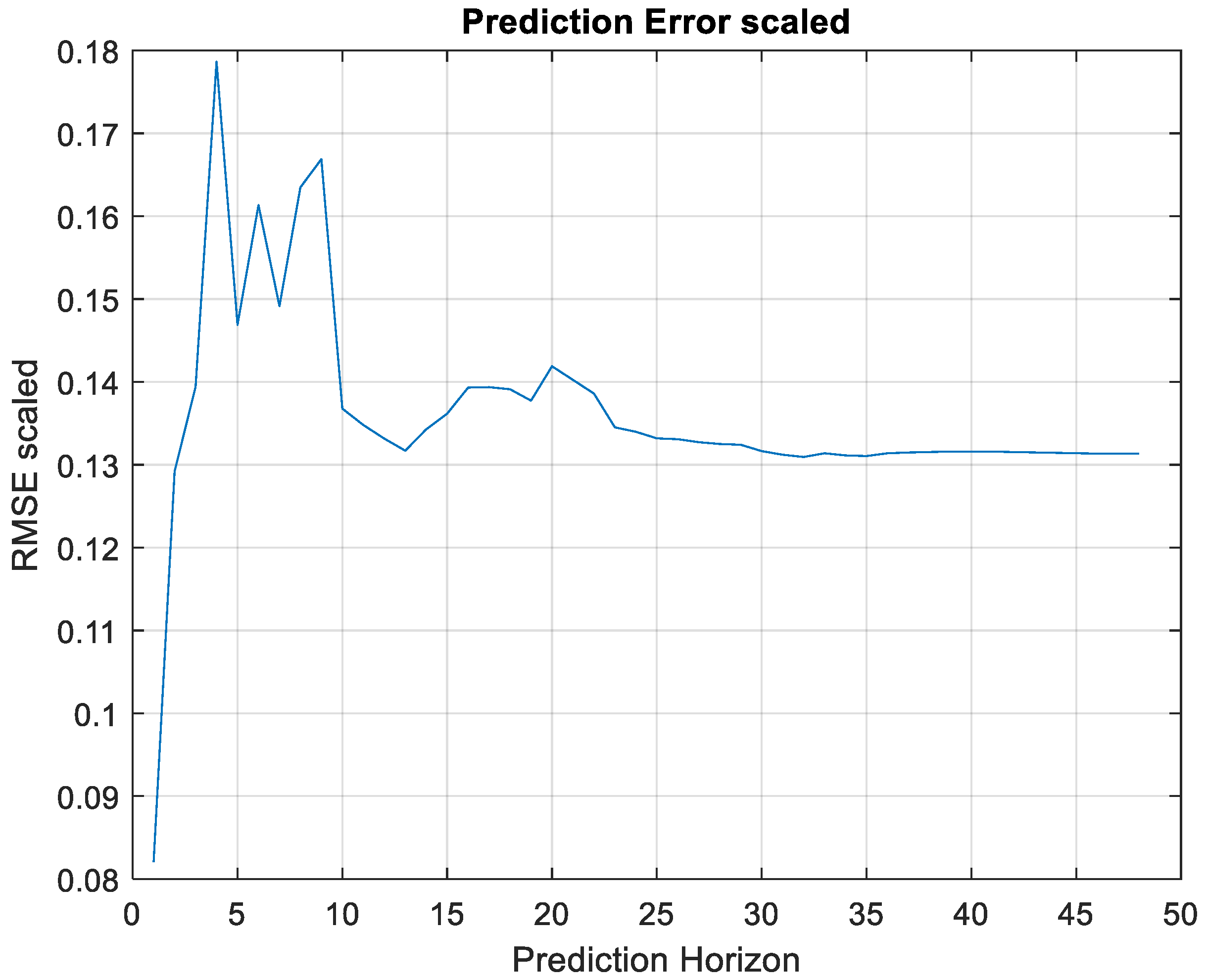
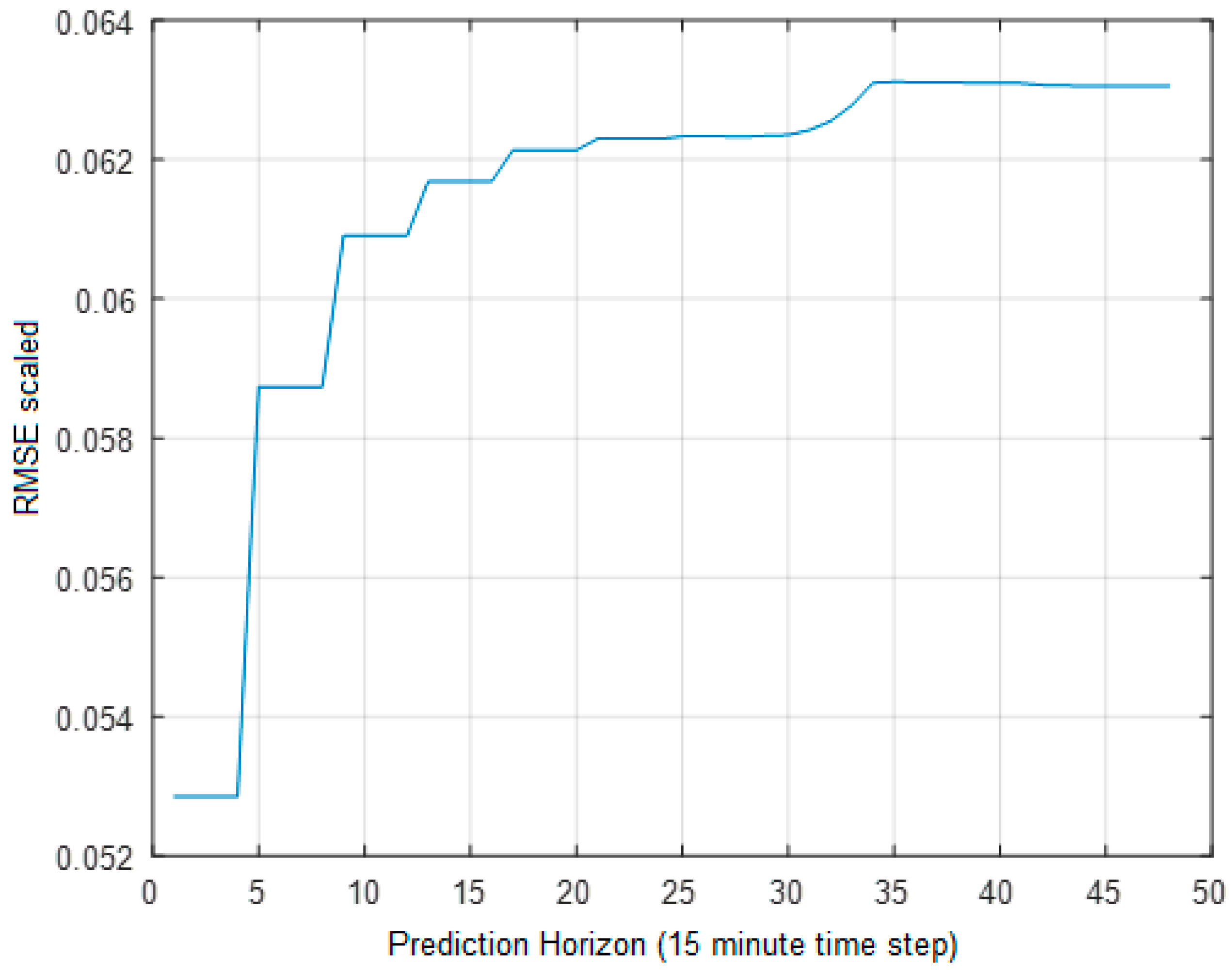
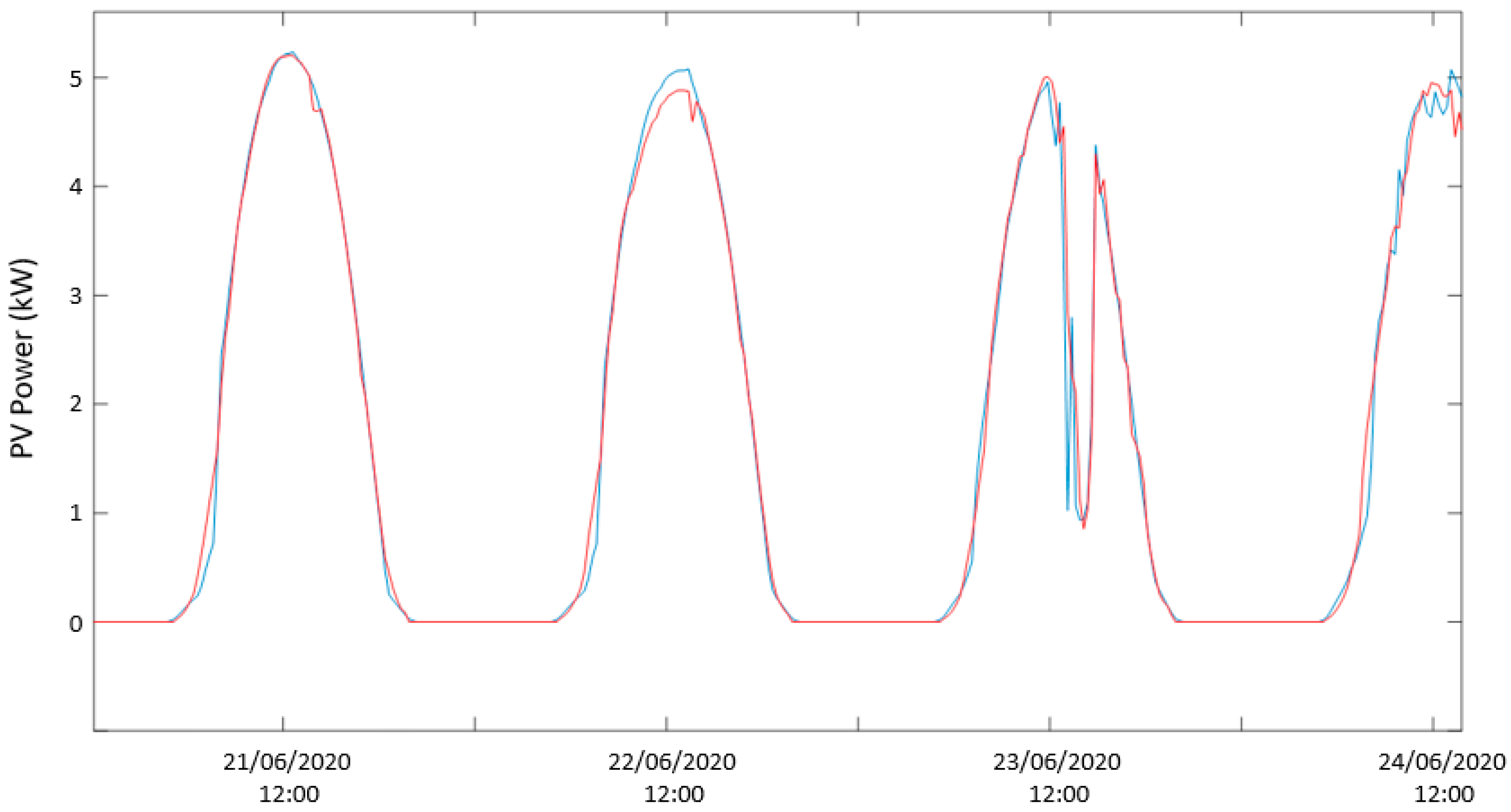
The evolution of the RMSE over the prediction horizon is shown in Figure 11, and the measured and one-step-ahead forecasted PV power are illustrated in Figure 12. The scaled RMSE varies from 0.053 to 0.063, which are excellent results. From the 20th step-ahead to the 48th step-ahead, the variation is minimum.
As is possible to see in Figure 11, the predicted values are very similar to the measured values in most points, with the most noticeable difference in a valley presented in the third day.
The results obtained were considered excellent, which did not justify using a second MOGA execution or the use of a model ensemble.
The one-step-ahead results obtained with the cascade of the three MOGA designed RBF models was compared to a baseline method, a persistent model (20):
This model was applied to the whole design data, achieving an RMSE of 0.25, approximately four times higher than the training, testing and validation RMSEs shown in Table 8.
5. Discussion
For assessing the quality of the forecasting results obtained with the proposed approach, they should be compared with the results achieved with the works referenced in Table 1. It should be noted that a completely fair comparison is not possible, as data used in these works are all different, the prediction horizons are not the same, and the majority of the papers only supply one-step-ahead predictions.
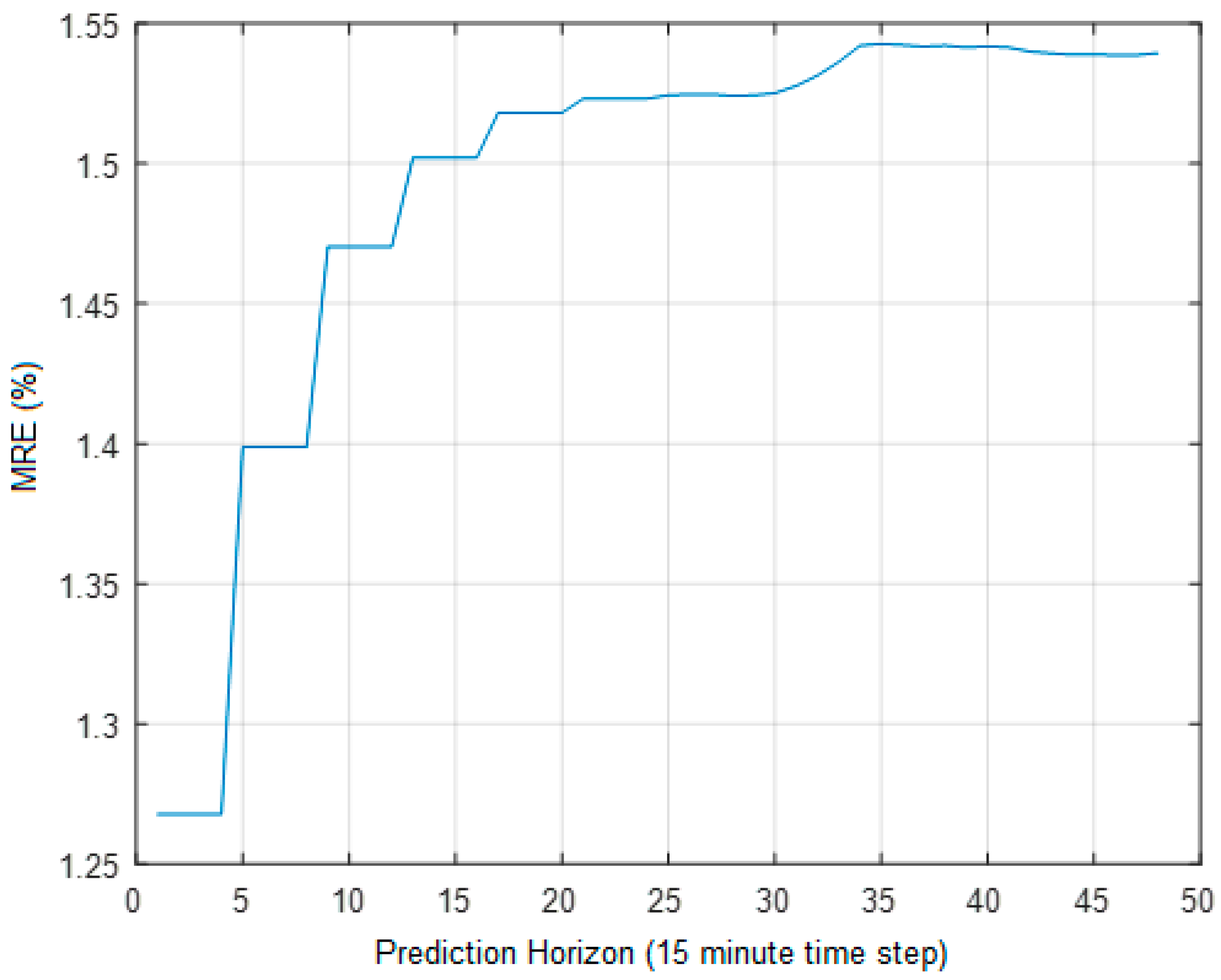
The only work that achieves multi-step forecasts is [27], employing a direct mode. This work uses 12 models that output forecasts with a time-step of 5 min, supplying forecasts between 5 min and 1 h. The MRE reported ranged from 4.2 to 9.3%. The MRE values obtained by our approach are shown in Figure 13.
The MRE obtained 1 h ahead in [27] is 9.3%. Our approach achieves a value of 1.3% for the same prediction horizon, which is seven times smaller.
All the other works only supply one-step-ahead forecasts. A comparison of the results obtained with the multi-step-ahead forecast is not fair to our approach, especially when one-step-ahead forecasts correspond to many steps-ahead of the multi-step forecasts. However, this is what will be done as there is no other alternative.
The work presented in [25] achieves an MRE of 3.3% for a PH of 1 day. In our work, the 48-steps forecasts correspond only to 12 h, with a value of 1.5%. Assuming that a 96 steps prediction would follow the same trend of Figure 12, our approach would obtain a smaller MRE.
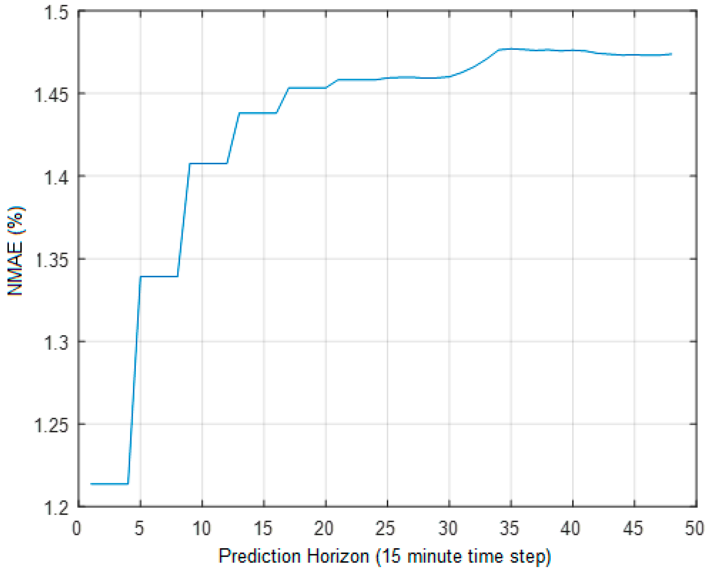
The work presented in [12] achieves NMAE values between 5.2 to 13.2% for a Prediction Horizon between 25 and 48 h ahead. Considering a rated power of 6 kW, this work’s approach obtains NMAE evolutions shown in Figure 14, this is, below 1.5%.
Again, speculating that a higher number of steps prediction would follow the same trend of Figure 10, our approach would obtain a smaller NMAE.
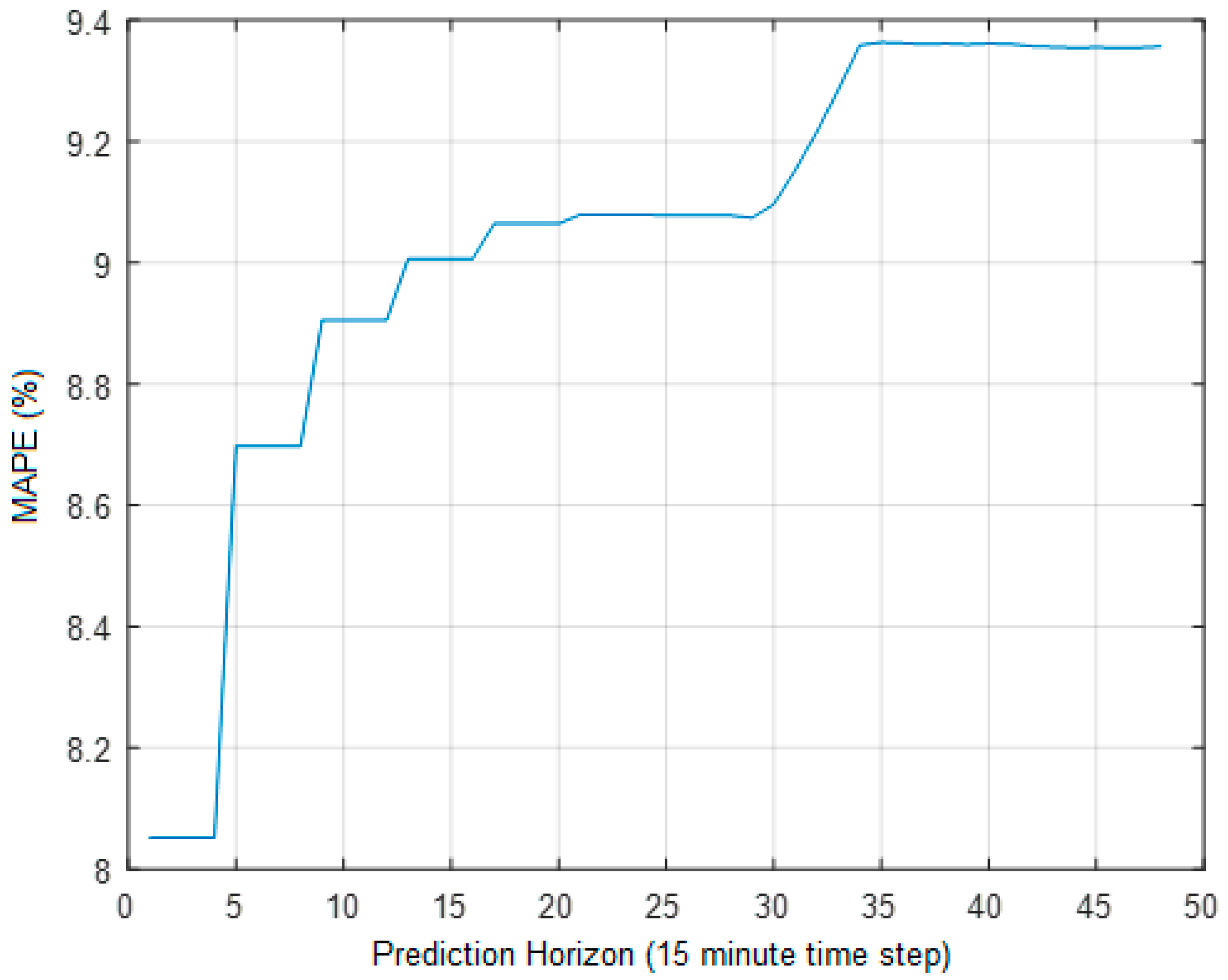
The work presented in [30] supplies forecasts of up to 1 h, with MAPE values between 24.7% and 37.8%. The MAPE values obtained with our approach are shown in Figure 15. For a 1-h forecast (four-steps-ahead) the MAPE is 8.0%.
In [31], the MAPE criterion is also employed. For a 5 min forecast, MAPE ranges between 2.2% and 11.2%. In our approach, the MAPE for a 15 min forecast is 8.0%.
The work presented in [33] also employs the MAPE criterion. For summer months, for 6, 12, and 24 h the values obtained were 28.6%, 38.5% and 37.8%. In our approach, 9.1% and 9.4% were obtained for 6 and 12 h ahead.
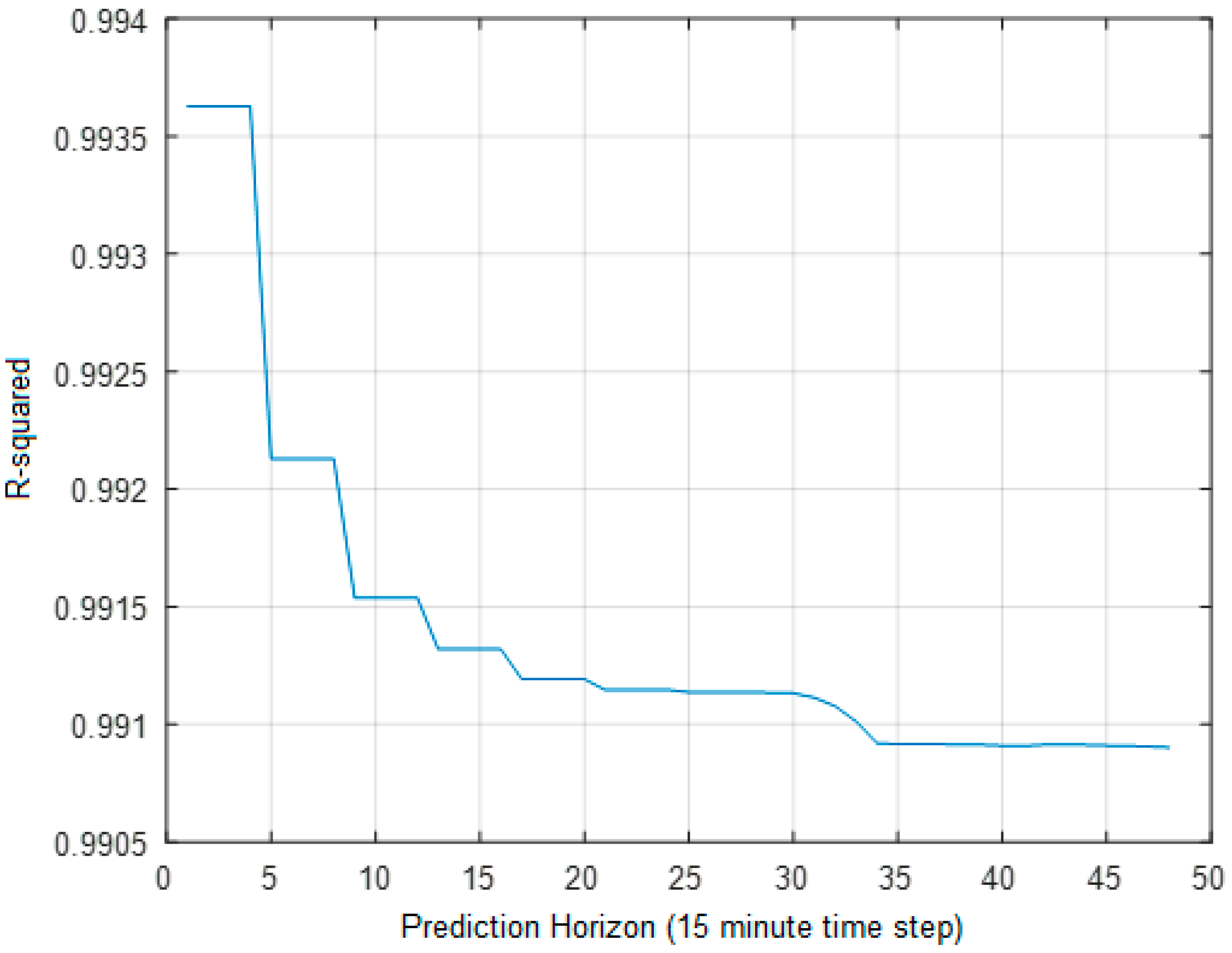
Work [28] shows their results in terms of the R-squared (R2) criterion. For a one-day forecast, the value obtained is 0.97. Figure 16 depicts the evolution of the coefficient of determination within the PH. Speculating again that a higher number of steps prediction would follow the same trend of Figure 16, our approach would obtain a much higher R2 value.
Work [32] uses a direct mode to supply multi-step ahead PV forecasts with a prediction horizon of 3 h, with steps of 15 min. Different models are designed for each season. For spring, summer, fall and winter, the coefficient of determination ranges from 0.998 to 0.918, 0.999 to 0.964, 0.996 to 0.907 and 0.997 to 0.905, respectively, between 15 min and 180 min ahead. Our second case uses data from spring and summer, with considerable better results.
To conclude the discussion, the authors would like to highlight that this predictive model is only one of the models necessary for our HEMS. Models of electric consumption were developed by the authors using the same methodology [30,33,44] and will be integrated into a MBPC HEMS scheme as the one described in [54]. Furthermore, in future studies the effect of dust on the PV panels will also to be considered, following the guidelines of [55], where an experimental analysis was developed for different dust types to evaluate their impact on the power output of the modules.
6. Conclusions
This work focused in PV electric power generation, designing for this purpose multi-step one-step-ahead forecasting models. The main goals were to improve the current PV power forecasting accuracy and, envisioning possible commercial use, to obtain the forecasts using only a few months of data. Two case studies were employed, the first using data from a specially built house in the USA, and the second based on a typical residence in Portugal’s Algarve region.
Excellent multi-step-ahead PV power forecasts were obtained with the methodology proposed. One-step values of MRE and NMAE of 1.25%, 8.0%, MAPE of 9.4%, R-squared of 0.994 were achieved, typically much better than results available in the literature. These were achieved using only a few months of design data were needed, in contrast with other works available in the literature.
In spite of the excellent quality of the models obtained, one should be aware that if this (fixed) model would be employed throughout the year, with different weather conditions, the forecasting performance would decrease. Fortunately, this can be alleviated if an adaptive mechanism is employed. This will shortly be applied to the PV power forecasting model.
The authors also note that this predictive model is only one of the models necessary for the HEMS that will be designed in the project in which this work is inserted. Models of electric consumption were also developed using the same methodology and in future works, they will be integrated into a MBPC HEMS scheme.
Author Contributions
All authors contributed equally to the investigation and writing of the paper. All authors have read and agreed to the published version of the manuscript.
Funding
The authors would like to acknowledge the support of Programa Operacional Portugal 2020 and Operational Program CRESC Algarve 2020 grant 01/SAICT/2018. Antonio Ruano acknowledges the support of Fundação para a Ciência e Tecnologia, through IDMEC, under LAETA, grant UIDB/50022/2020.
Institutional Review Board Statement
Not applicable
Informed Consent Statement
Not applicable
Data Availability Statement
The data presented in this study are available on request from the corresponding author.
Conflicts of Interest
The authors declare no conflict of interest.
References
- Antonanzas, J.; Osorio, N.; Escobar, R.; Urraca, R.; Martinez-de-Pison, F.J.; Antonanzas-Torres, F. Review of photovoltaic power forecasting. Sol. Energy 2016, 136, 78–111. [Google Scholar] [CrossRef]
- Stine, W.B.; Harrigan, R.W. Solar Energy Fundamentals and Design; John Wiley and Sons, Inc.: New York, NY, USA, 1985. [Google Scholar]
- Kong, H.; Sui, H.; Tang, J.; Zhang, P. Research Status and Difficulties of Ultra-short-term Prediction of Photovoltaic Power. IOP Conf. Ser. Earth Environ. Sci. 2019, 252, 32094. [Google Scholar] [CrossRef]
- Bianchini, G.; Pepe, D.; Vicino, A. Estimation of Photovoltaic Generation Forecasting Models using Limited Information. Automatica 2020, 113, 108688. [Google Scholar] [CrossRef] [Green Version]
- Sun, C.; Sun, F.; Moura, S.J. Nonlinear Predictive Energy Management of Residential Buildings with Photovoltaics & Batteries. J. Power Sources 2016, 325, 723–731. [Google Scholar]
- Coimbra, C.F.M.; Kleissl, J.; Marquez, R. Chapter 8: Overview of solar-forecasting methods and a metric for accuracy evaluation. In Solar Energy Forecasting and Resource Assessment; Elsevier Academic Press: Cambridge, MA, USA, 2013; pp. 171–194. [Google Scholar]
- Fahrenbruch, A.; Bube, R. Fundamentals of Solar Cells: Photovoltaic Solar Energy Conversion; Elsevier: Amsterdam, The Netherlands, 2012. [Google Scholar]
- Tiwari, G.N. Solar Energy: Fundamentals, Design, Modelling and Applications; Alpha Science Int’l Ltd.: Oxford, UK, 2002. [Google Scholar]
- McEvoy, A.; Markvart, T.; Castañer, L.; Markvart, T.; Castaner, L. Practical Handbook of Photovoltaics: Fundamentals and Applications; Elsevier: Amsterdam, The Netherlands, 2003. [Google Scholar]
- Diagne, M.; David, M.; Lauret, P.; Boland, J.; Schmutz, N. Review of Solar Irradiance Forecasting Methods and a Proposition for Small-Scale Insular Grids. Renew. Sustain. Energy Rev. 2013, 27, 65–76. [Google Scholar] [CrossRef] [Green Version]
- Ferreira, P.M.; Gomes, J.M.; Martins, I.A.C.; Ruano, A.E. A Neural Network based Intelligent Predictive Sensor for Cloudiness, Solar Radiation, and Air Temperature. Sensors 2012, 12, 15750–15777. [Google Scholar] [CrossRef]
- Leva, S.; Dolara, A.; Grimaccia, F.; Mussetta, M.; Ogliari, E. Analysis and Validation of 24 Hours Ahead Neural Network Forecasting of Photovoltaic Output Power. Math. Comput. Simul. 2017, 131, 88–100. [Google Scholar] [CrossRef] [Green Version]
- Law, E.W.; Kay, M.; Taylor, R.A. Calculating the Financial Value of a Concentrated Solar Thermal Plant Operated using Direct Normal Irradiance Forecasts. Sol. Energy 2016, 125, 267–281. [Google Scholar] [CrossRef] [Green Version]
- Voyant, C.; Notton, G.; Kalogirou, S.; Nivet, M.-L.; Paoli, C.; Motte, F.; Fouilloy, A. Machine Learning Methods for Solar Radiation Forecasting: A Review. Renew. Energy 2017, 105, 569–582. [Google Scholar] [CrossRef]
- Mohanty, S.; Patra, P.K.; Sahoo, S.S. Prediction and Application of Solar Radiation with Soft Computing Over Traditional and Conventional Approach–A Comprehensive Review. Renew. Sustain. Energy Rev. 2016, 56, 778–796. [Google Scholar] [CrossRef]
- Qazi, A.; Fayaz, H.; Wadi, A.; Raj, R.G.; Rahim, N.A.; Khan, W.A. The Artificial Neural Network for Solar Radiation Prediction and Designing Solar Systems: A Systematic Literature Review. J. Clean. Prod. 2015, 104, 1–12. [Google Scholar] [CrossRef]
- Yadav, A.K.; Chandel, S.S. Solar Radiation Prediction Using Artificial Neural Network Techniques: A Review. Renew. Sustain. Energy Rev. 2014, 33, 772–781. [Google Scholar] [CrossRef]
- Law, E.W.; Prasad, A.A.; Kay, M.; Taylor, R.A. Direct Normal Irradiance Forecasting and its Application to Concentrated Solar Thermal Output Forecasting—A Review. Sol. Energy 2014, 108, 287–307. [Google Scholar] [CrossRef]
- Das, U.K.; Tey, K.S.; Seyedmahmoudian, M.; Mekhilef, S.; Idris, M.Y.I.; Van Deventer, W.; Horan, B.; Stojcevski, A. Forecasting of Photovoltaic Power Generation and Model Optimization: A Review. Renew. Sustain. Energy Rev. 2018, 81, 912–928. [Google Scholar] [CrossRef]
- Foucquier, A.; Robert, S.; Suard, F.; Stéphan, L.; Jay, A. State of the art in Building Modelling and Energy Performances Prediction: A review. Renew. Sustain. Energy Rev. 2013, 23, 272–288. [Google Scholar] [CrossRef] [Green Version]
- Killian, M.; Kozek, M. Ten Questions Concerning Model Predictive Control for Energy Efficient Buildings. Build. Environ. 2016, 105, 403–412. [Google Scholar] [CrossRef]
- Sobri, S.; Koohi-Kamali, S.; Rahim, N.A. Solar Photovoltaic Generation Forecasting Methods: A Review. Energy Convers. Manag. 2018, 156, 459–497. [Google Scholar] [CrossRef]
- Raza, M.Q.; Nadarajah, M.; Ekanayake, C. On Recent Advances in PV Output Power Forecast. Sol. Energy 2016, 136, 125–144. [Google Scholar] [CrossRef]
- Ruano, A.E.; Ferreira, P.M.; Fonseca, C.M. An Overview of Nonlinear Identification and Control with Neural Networks. In Intelligent Control Systems using Computational Intelligence Techniques; Ruano, A.E., Ed.; Institution of Electrical Engineers: London, UK, 2005; Volume 70, pp. 37–87. [Google Scholar]
- Yang, H.; Huang, C.; Huang, Y.; Pai, Y. A Weather-Based Hybrid Method for 1-Day Ahead Hourly Forecasting of PV Power Output. IEEE Trans. Sustain. Energy 2014, 5, 917–926. [Google Scholar] [CrossRef]
- Cervone, G.; Clemente-Harding, L.; Alessandrini, S.; Delle Monache, L. Short-term photovoltaic power forecasting using Artificial Neural Networks and an Analog Ensemble. Renew. Energy 2017, 108, 274–286. [Google Scholar] [CrossRef] [Green Version]
- Rana, M.; Koprinska, I.; Agelidis, V.G. Univariate and multivariate methods for very short-term solar photovoltaic power forecasting. Energy Convers. Manag. 2016, 121, 380–390. [Google Scholar] [CrossRef]
- Alomari, M.H.; Adeeb, J.; Younis, O. Solar photovoltaic power forecasting in jordan using artificial neural networks. Int. J. Electr. Comput. Eng. 2018, 8, 497. [Google Scholar] [CrossRef]
- Wang, F.; Zhang, Z.; Liu, C.; Yu, Y.; Pang, S.; Duić, N.; Shafie-khah, M.; Catalão, J.P.S. Generative adversarial networks and convolutional neural networks based weather classification model for day ahead short-term photovoltaic power forecasting. Energy Convers. Manag. 2019, 181, 443–462. [Google Scholar] [CrossRef]
- Zhou, H.; Zhang, Y.; Yang, L.; Liu, Q.; Yan, K.; Du, Y. Short-Term Photovoltaic Power Forecasting Based on Long Short Term Memory Neural Network and Attention Mechanism. IEEE Access 2019, 7, 78063–78074. [Google Scholar] [CrossRef]
- Wang, K.; Qi, X.; Liu, H. A comparison of day-ahead photovoltaic power forecasting models based on deep learning neural network. Appl. Energy 2019, 251, 113315. [Google Scholar] [CrossRef]
- Li, G.; Xie, S.; Wang, B.; Xin, J.; Li, Y.; Du, S. Photovoltaic Power Forecasting With a Hybrid Deep Learning Approach. IEEE Access 2020, 8, 175871–175880. [Google Scholar] [CrossRef]
- Hossain, M.S.; Mahmood, H. Short-Term Photovoltaic Power Forecasting Using an LSTM Neural Network and Synthetic Weather Forecast. IEEE Access 2020, 8, 172524–172533. [Google Scholar] [CrossRef]
- Zhang, J.; Florita, A.; Hodge, B.-M.; Lu, S.; Hamann, H.F.; Banunarayanan, V.; Brockway, A.M. A suite of metrics for assessing the performance of solar power forecasting. Sol. Energy 2015, 111, 157–175. [Google Scholar] [CrossRef] [Green Version]
- Khosravani, H.R.; Ruano, A.E.; Ferreira, P.M. A convex hull-based data selection method for data driven models. Appl. Soft Comput. 2016, 47, 515–533. [Google Scholar] [CrossRef]
- Levenberg, K. A method for the solution of certain non-linear problems in least squares. Q. Appl. Math. 1944, 2, 164–168. [Google Scholar] [CrossRef] [Green Version]
- Marquardt, D.W. An algorithm for least-squares estimation of nonlinear parameters. J. Soc. Ind. Appl. Math. 1963, 11, 431–441. [Google Scholar] [CrossRef]
- Ruano, A.E.B.; Jones, D.I.; Fleming, P.J. A New Formulation of the Learning Problem for a Neural Network Controller. In Proceedings of the 30th IEEE Conference on Decision and Control, Brighton, UK, 11–13 December 1991; pp. 865–866. [Google Scholar]
- Ferreira, P.M.; Ruano, A.E. Application of Computational Intelligence Methods to Greenhouse Environmental Modelling. In Proceedings of the IEEE International Joint Conference on Neural Networks (IJCNN’08), Hong Kong, China, 1–8 June 2008; pp. 3582–3589. [Google Scholar]
- Ferreira, P.M.; Ruano, A.E.; Pestana, R.; Koczy, L.T. Evolving RBF predictive models to forecast the Portuguese electricity consumption. IFAC Proc. Vol. 2009, 42, 414–419. [Google Scholar] [CrossRef]
- Hajimani, E.; Ruano, M.G.; Ruano, A.E. An intelligent support system for automatic detection of cerebral vascular accidents from brain CT images. Comput. Methods Programs Biomed. 2017, 146, 109–123. [Google Scholar] [CrossRef] [PubMed]
- Khosravani, H.; Castilla, M.; Berenguel, M.; Ruano, A.; Ferreira, P. A Comparison of Energy Consumption Prediction Models Based on Neural Networks of a Bioclimatic Building. Energies 2016, 9, 57. [Google Scholar] [CrossRef] [Green Version]
- Ruano, A.E.; Pesteh, S.; Silva, S.; Duarte, H.; Mestre, G.; Ferreira, P.M.; Khosravani, H.R.; Horta, R. The IMBPC HVAC system: A complete MBPC solution for existing HVAC systems. Energy Build. 2016, 120, 145–158. [Google Scholar] [CrossRef]
- Al-Dahidi, S.; Ayadi, O.; Alrbai, M.; Adeeb, J. Ensemble Approach of Optimized Artificial Neural Networks for Solar Photovoltaic Power Prediction. IEEE Access 2019, 7, 81741–81758. [Google Scholar] [CrossRef]
- Honda. Honda Smart Home US. Available online: https://www.hondasmarthome.com/ (accessed on 21 December 2020).
- Ferreira, P.M.; Ruano, A.E. Exploiting the separability of linear and nonlinear parameters in radial basis function networks. In Proceedings of the Adaptive Systems for Signal Processing, Communications, and Control Symposium (AS-SPCC), Lake Louise, AB, Canada, 1–4 October 2000; pp. 321–326. [Google Scholar]
- Chinrungrueng, C.; Sequin, C.H. Optimal adaptive k-means algorithm with dynamic adjustment of learning rate. IEEE Trans. Neural Netw. 1995, 6, 157–169. [Google Scholar] [CrossRef]
- Peel, M.C.; Finlayson, B.L.; McMahon, T.A. Updated world map of the Köppen-Geiger climate classification. Hydrol. Earth Syst. Sci. 2007, 11, 1633–1644. [Google Scholar] [CrossRef] [Green Version]
- Rubel, F.; Kottek, M. Observed and projected climate shifts 1901-2100 depicted by world maps of the Köppen-Geiger climate classification. Meteorol. Z. 2010, 19, 135–141. [Google Scholar] [CrossRef] [Green Version]
- Europe-Solar-Store. Sharp NU-AK300. Available online: https://www.europe-solarstore.com/sharp-nu-ak300.html (accessed on 21 December 2020).
- Kostal. Plenticore Plus. Available online: https://www.kostal-solar-electric.com/en-gb/products/hybrid-inverters/plenticore-plus (accessed on 21 December 2020).
- Eft, S. Battery Box HV. Available online: https://www.eft-systems.de/en/TheB-BOX/product/BatteryBoxHV/3 (accessed on 21 December 2020).
- Mestre, G.; Ruano, A.; Duarte, H.; Silva, S.; Khosravani, H.; Pesteh, S.; Ferreira, P.; Horta, R. An Intelligent Weather Station. Sensors 2015, 15, 31005–31022. [Google Scholar] [CrossRef]
- Ju, Y.; Li, J.; Sun, G. Ultra-Short-Term Photovoltaic Power Prediction Based on Self-Attention Mechanism and Multi-Task Learning. IEEE Access 2020, 8, 44821–44829. [Google Scholar] [CrossRef]
- Hussain, A.; Batra, A.; Pachauri, R. An experimental study on effect of dust on power loss in solar photovoltaic module. Renew. Wind Water Solar 2017, 4, 9. [Google Scholar] [CrossRef]
Figure 1.
Methodology steps.

Figure 2.
The architecture of the Honda Smart Home US [45].
Figure 2.
The architecture of the Honda Smart Home US [45].

Figure 3.
Root mean square errors (RMSEs) of the scaled photovoltaic (PV) power for (a), (b) and (c) model configurations.
Figure 3.
Root mean square errors (RMSEs) of the scaled photovoltaic (PV) power for (a), (b) and (c) model configurations.

Figure 4.
Honda Smart Home (HSH) model lags.

Figure 5.
RMSEs of the scaled PV power within the prediction horizon.

Figure 6.
PV system: (a,b): photovoltaic panels; (c) inverter; (d) storage.

Figure 7.
RMSEs of the scaled air temperature within the prediction horizon.

Figure 8.
Measured (blue) and one-step-ahead forecast (red) solar irradiance for four selected days.
Figure 8.
Measured (blue) and one-step-ahead forecast (red) solar irradiance for four selected days.

Figure 9.
RMSEs of the scaled air temperature within the prediction horizon.

Figure 10.
Measured (blue) and one-step-ahead forecast (red) air temperature for four selected days.
Figure 10.
Measured (blue) and one-step-ahead forecast (red) air temperature for four selected days.

Figure 11.
RMSEs of the scaled PV power within the prediction horizon.

Figure 12.
Measured (blue) and one-step-ahead forecast (red) DC PV power for four selected days.

Figure 13.
Mean relative error (MRE, %) of the PV power within the prediction horizon.

Figure 14.
Normalized mean absolute error (NMAE, in %) of the PV power within the prediction horizon.
Figure 14.
Normalized mean absolute error (NMAE, in %) of the PV power within the prediction horizon.

Figure 15.
MAPE (in %) of the PV power within the prediction horizon.

Figure 16.
Coefficient of determination of the PV power within the prediction horizon.


Table 1.
Related works.
| Source | Method | PH | Sampling Time | Exogenous Variables | Accuracy |
|---|---|---|---|---|---|
| [25] | Hybrid Method | 1 Day | 1 h | Solar irradiance, month, maximum temperature, probability of precipitation, verbal weather description | MRE = 3.3% |
| [12] | MLP | 25–48 h | 1 h | Solar irradiance, weather forecasts | NMAE = 5.2–13.2% |
| [27] | MLP | 5–60 min | 5 min | Solar irradiance, atmospheric temperature and relative humidly, and wind speed | MRE = 4.2–9.3% |
| [28] | MLP | 1 Day | 1 h | Solar irradiance | R2 = 0.97 |
| [30] | LSTM | 7.5 min | Atmospheric temperature | MAPE = 24.7–37.8% | |
| [31] | Deep learning | Up to 1 h | 5 min | Atmospheric temperature, solar irradiance | MAPE = 2.2% to 11.2% |
| [32] | NNs CNN and LSTM | 5 min | 15–180 min | - | R2 = 0.998–0.906 |
| [33] | LSTM | 15–180 min | 6, 12, and 24 h | Solar irradiance, temperature, wind speed, precipitable water, relative humidity and pressure | MAPE = 28.5% to 37.8% |
Table 2.
Performance for the non-dominated sets.
| εtr | εte | εva | εp |
|---|---|---|---|
| 0.08 | 0.07 | 0.07 | 3.95 |
Table 3.
Selected model results.
| Features | Neurons | εtr | εte | εva | εp |
|---|---|---|---|---|---|
| 19 | 20 | 0.07 | 0.07 | 0.07 | 4.23 |
Table 4.
Performance statistics for the non-dominated set.
| Training | Testing | Validation | |
|---|---|---|---|
| 1.0 | 0.7 | 0.8 | |
| 1.3 | 0.8 | 0.9 | |
| 1.9 | 1.2 | 1.3 |
Table 5.
Selected model results.
| Features | Neurons | εtr | εte | εva | εp |
|---|---|---|---|---|---|
| 12 | 18 | 0.12 | 0.07 | 0.12 | 6.84 |
Table 6.
Performance statistics for the non-dominated set.
| Training | Testing | Validation | |
|---|---|---|---|
| 2.7 | 2.5 | 2.6 | |
| 2.9 | 2.6 | 2.7 | |
| 11.8 | 39 | 39.6 |
Table 7.
Selected model results.
| Features | Neurons | εtr | εte | εva | εp |
|---|---|---|---|---|---|
| 18 | 15 | 0.028 | 0.027 | 0.027 | 7.04 |
Table 8.
Performance statistics for the non-dominated set.
| Training | Testing | Validation | |
|---|---|---|---|
| 1.5 | 0.6 | 0.5 | |
| 4.3 | 3.8 | 4.3 | |
| 6.8 | 4.4 | 4.7 |
Table 9.
Selected model results.
| Features | Neurons | εtr | εte | εva | εp |
|---|---|---|---|---|---|
| 10 | 16 | 0.07 | 0.05 | 0.06 | 2.91 |
Publisher’s Note: MDPI stays neutral with regard to jurisdictional claims in published maps and institutional affiliations. |
© 2021 by the authors. Licensee MDPI, Basel, Switzerland. This article is an open access article distributed under the terms and conditions of the Creative Commons Attribution (CC BY) license (http://creativecommons.org/licenses/by/4.0/).
Share and Cite
MDPI and ACS Style
Bot, K.; Ruano, A.; Ruano, M.d.G. Short-Term Forecasting Photovoltaic Solar Power for Home Energy Management Systems. Inventions 2021, 6, 12. https://0-doi-org.brum.beds.ac.uk/10.3390/inventions6010012
AMA Style
Bot K, Ruano A, Ruano MdG. Short-Term Forecasting Photovoltaic Solar Power for Home Energy Management Systems. Inventions. 2021; 6(1):12. https://0-doi-org.brum.beds.ac.uk/10.3390/inventions6010012
Chicago/Turabian StyleBot, Karol, Antonio Ruano, and Maria da Graça Ruano. 2021. "Short-Term Forecasting Photovoltaic Solar Power for Home Energy Management Systems" Inventions 6, no. 1: 12. https://0-doi-org.brum.beds.ac.uk/10.3390/inventions6010012