A Study of the Mixing Performance of Different Impeller Designs in Stirred Vessels Using Computational Fluid Dynamics

College of Engineering, Nanjing Agricultural University Jiangsu Province, Nanjing 210031, China
*
Author to whom correspondence should be addressed.
Designs 2018, 2(1), 10; https://0-doi-org.brum.beds.ac.uk/10.3390/designs2010010
Submission received: 8 January 2018
/
Revised: 6 March 2018
/
Accepted: 6 March 2018
/
Published: 8 March 2018
(This article belongs to the Special Issue Challenges and Progress in Turbomachinery Design)
Abstract
:Design and operation of mixing systems using agitated vessels is a difficult task due to the challenge of obtaining accurate information on impeller-induced turbulence. The use of Computational Fluid Dynamics (CFD) can provide detailed understanding of such systems. In this study, experimental tests and computational fluid dynamics simulations were performed to examine the flow characteristics of four impeller designs (anchor, saw-tooth, counter-flow and Rushton turbine), in achieving solution homogeneity. The impellers were used to mix potassium sulfate granules, from which values of electrical conductivity of the solution were measured and used to estimate the distribution pattern of dissolved solid concentrations within the vessel. CFD models were developed for similar mixing arrangement using commercial software, ANSYS Fluent 18.1 solver and the standard k-epsilon (ε) turbulence model. The Multiple Reference Frame (MRF) approach was used to simulate the impeller rotation. Velocity profiles generated from the simulations were in good agreement with the experimental predictions, as well as with results from previous studies. It was concluded that, through CFD analysis, detailed information can be obtained for optimal design of mixing apparatus. These findings are relevant in choosing the best mixing equipment and provides a basis for scaling up mixing operations in larger systems.
1. Introduction
Mixing is an essential operation in many engineering fields. It has central significance in food processing, pharmaceutical production, chemical engineering, biotechnology, agri-chemical preparations, paint manufacturing, water purification among countless other applications [1]. Many mixing schemes using stirred tanks have been developed to meet various production and processing goals [2]. In agricultural systems, mixing set-ups have been used in a number of processes, such as preparing farm chemical concentrations, balancing nutrient amounts in fertilizer tanks, blending different substances and processing farm products.
One of the main aims of agitation systems using stirred vessels is to maintain balanced quantities of substances in different phases based on concentration levels [3]. In cases where soluble solids are mixed, stirrers are used to increase interaction between the particles and avoid uneven accumulation at one point [4]. Flow streams in stirred vessels are known to be turbulent, chaotic and difficult to determine; therefore attaining homogeneity in such mixing processes is a demanding task. Achieving uniform concentrations of mixing products is paramount for efficient and economical use of the expensive chemicals, fertilizers and other mixing agents in agricultural applications. A careful choice of equipment that generates sufficient turbulence and flow in the mixing vessel is therefore necessary.
The inconsistencies in mixing quality can be attributed to the lack of a clear understanding of the mixing processes due to the complex nature of impeller-induced turbulence in agitated vessels [5,6]. There is a need for in-depth studies to determine mixing efficiency and accurately predict the overall performance of these systems. It has been established that the performance of mixing processes is a product of the mixing time, the type of impeller used, number of impeller blades, blade size, working angular speeds, and vessel configurations [7].
In large-scale mixing plants, stirrers and the entire agitation set-up should be able to create faster movement of substances and high turbulence. This makes the entire mixing process in large containers complicated and impractical to study through experiments [8]. There is therefore a need to provide a more workable method that will simplify the process.
Computational fluid dynamics (CFD) is instrumental in analyzing fluid flow systems using numerical methods and simulations in computer-controlled programs [9]. With CFD, engineers can easily study new and complex models in virtual environments, determine the design details, predict possible sources of failure and optimize system operations. Simulations have been used to investigate the hydrodynamics of many industrial processes and aeronautics among other numerous fields [10]. Furthermore, many researchers and industrialists have found the use of CFD helpful in reducing the cost and time spent in creating large and complicated prototypes of trial systems. Using CFD technique, satisfactory and crucial information can be obtained within a small working area and with less effort.
In order to achieve excellent mixing results, CFD can be employed as a tool for gaining in-depth knowledge of the turbulent dynamics of mixing operations in stirred vessels. Through numerical simulations, the effects of diverse and irregular configurations of mixing tanks, impeller designs and baffles can be modelled. The expected performance of using atypically large vessels [11] and under extreme working conditions can also be projected. Some of the mixing parameters that have been investigated using numerical methods in CFD include mixing times, power requirements, flow types, and velocity patterns [12].
Since impeller design is the most important component for determining the performance of mechanically agitated mixers [13], its design features and operational characteristics can be described theoretically using CFD. Several researchers have performed CFD tests to examine the effects of impeller type in mixing vessels. Cokljat et al. [14,15,16] did simulations of impeller flow behavior in stirred tanks using CFD in order to study flow velocities and mixing time. Tatterson [17] emphasized the importance of numerically modelling precise impeller flow characteristics.
The objective of this work was to use CFD technique alongside experimental tests to study the mixing behavior of different impeller designs. This will add to the knowledge necessary for choosing the best mixing designs. It was also expected that this work would give a justifiable basis for accurate scale-up of mixing systems in industrial, field, and agricultural mixing operations.
In this study, four different types of impellers: anchor, counter-flow, saw-tooth, and Rushton turbine impellers were designed and studied to determine how their distinct design features affected flow characteristics in a stirred vessel. Experimental tests were performed to provide a comparative reference to the simulation results. Velocity profiles generated in CFD were interpreted as the impeller flow characteristics. Simulations were done using commercial software, ANSYS Fluent 18.1 solver. The standard k-epsilon (ε) model was used to set up the turbulent flow process and the multiple reference frames (MRF) approach used to model the impeller motion in a baffled tank.
2. Materials and Methods
Experiments were conducted in the engineering laboratory of Nanjing Agricultural University in the month of August 2017, at room temperature and pressure. Four distinct, top-entering agitation impeller designs were used to dissolve solid granules of potassium sulfate (K2SO4) in water. Electrical Conductivity (EC) measurements of the mixed solutions from different locations in the liquid volume were used to predict the individual impeller performance.
2.1. Experimental Set-Up
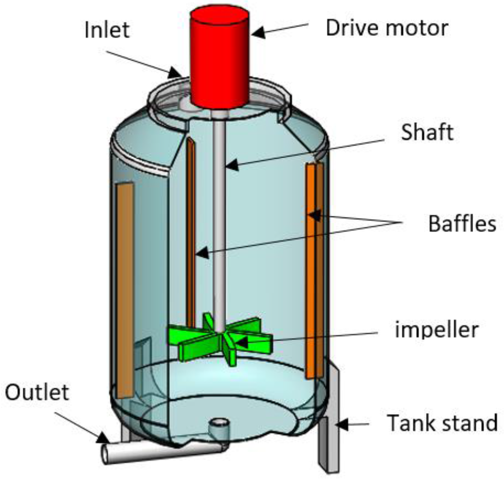
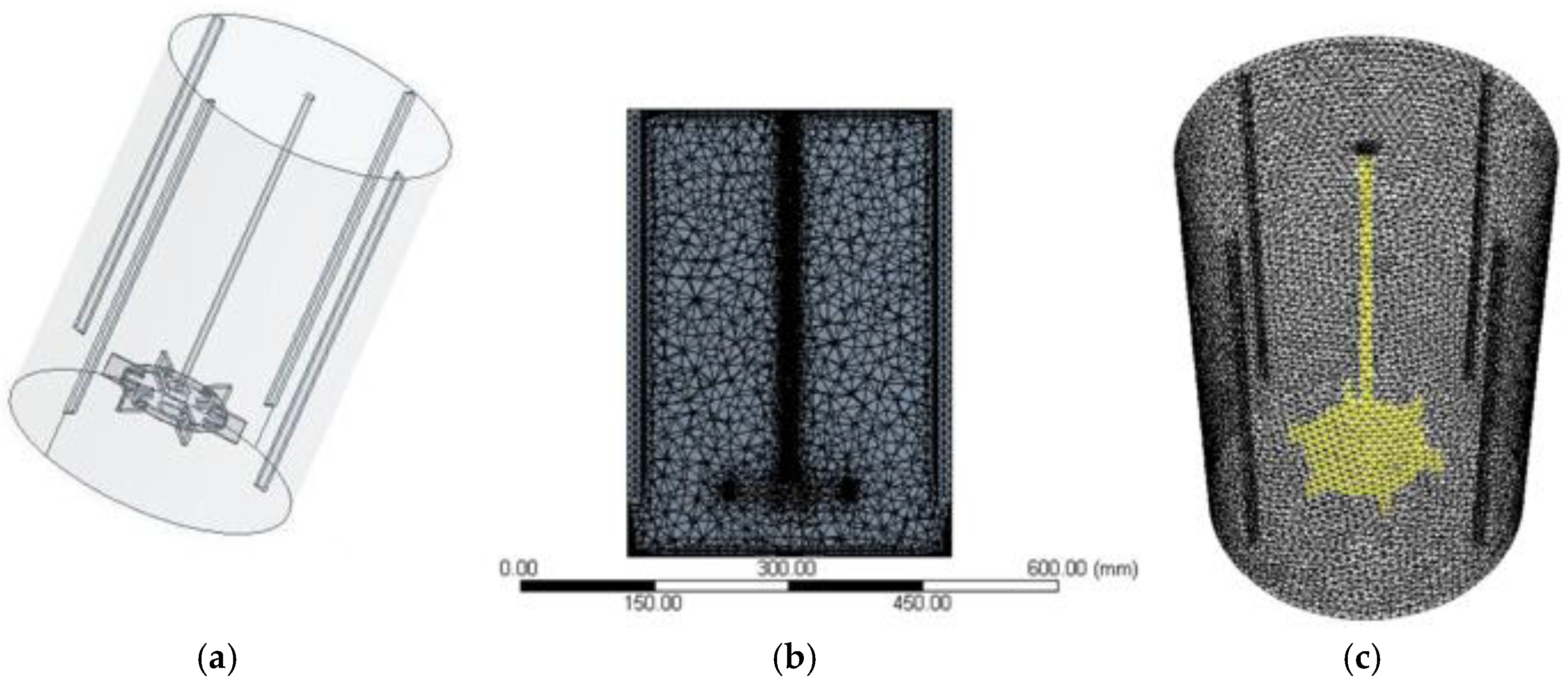
A cylindrical tank with four baffles arranged symmetrically on the tank’s inner walls was designed for the experiment. Figure 1 below shows the experimental tank, with one baffle cut off to show the inner apparatus.
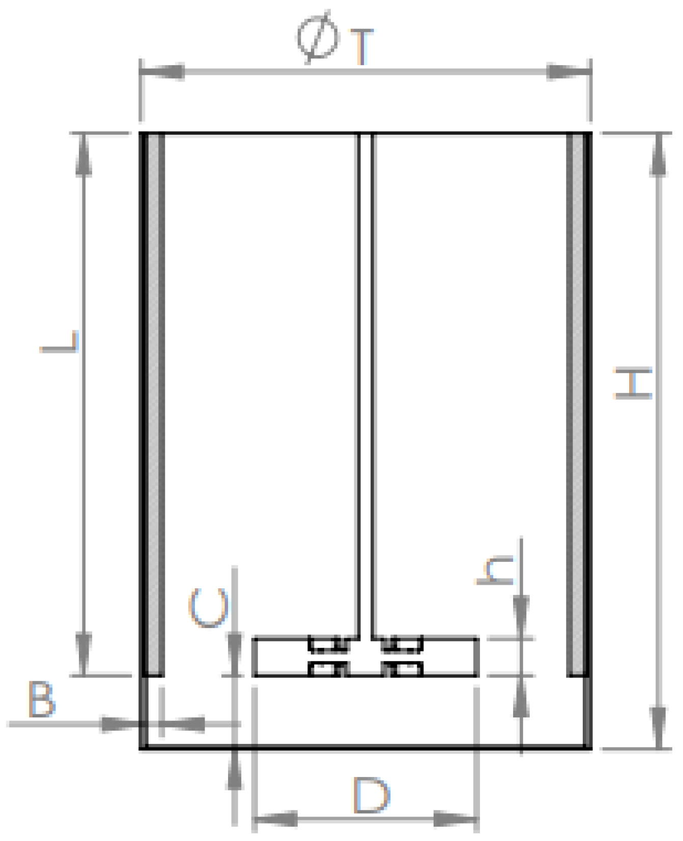
The shaft holding the impellers had a diameter of 0.012 m and were positioned concentric to the axis of the tank. Baffles were included in the set-up to prevent the liquid from spinning as a single body. The outline of the experimental tank and the dimensions of the agitation components are shown in Figure 2 and Table 1 respectively.
An electric mixer (M12 + 70 cm, Wuyi Mingcheng Co., Hengshui City, China) with a capacity of 220 V, 50 Hz, 1050 W and six adjustable speeds of between 100–600 rpm was used to run the impellers. Water was filled into the tank up to the 500 mm mark so that all baffles were submerged.
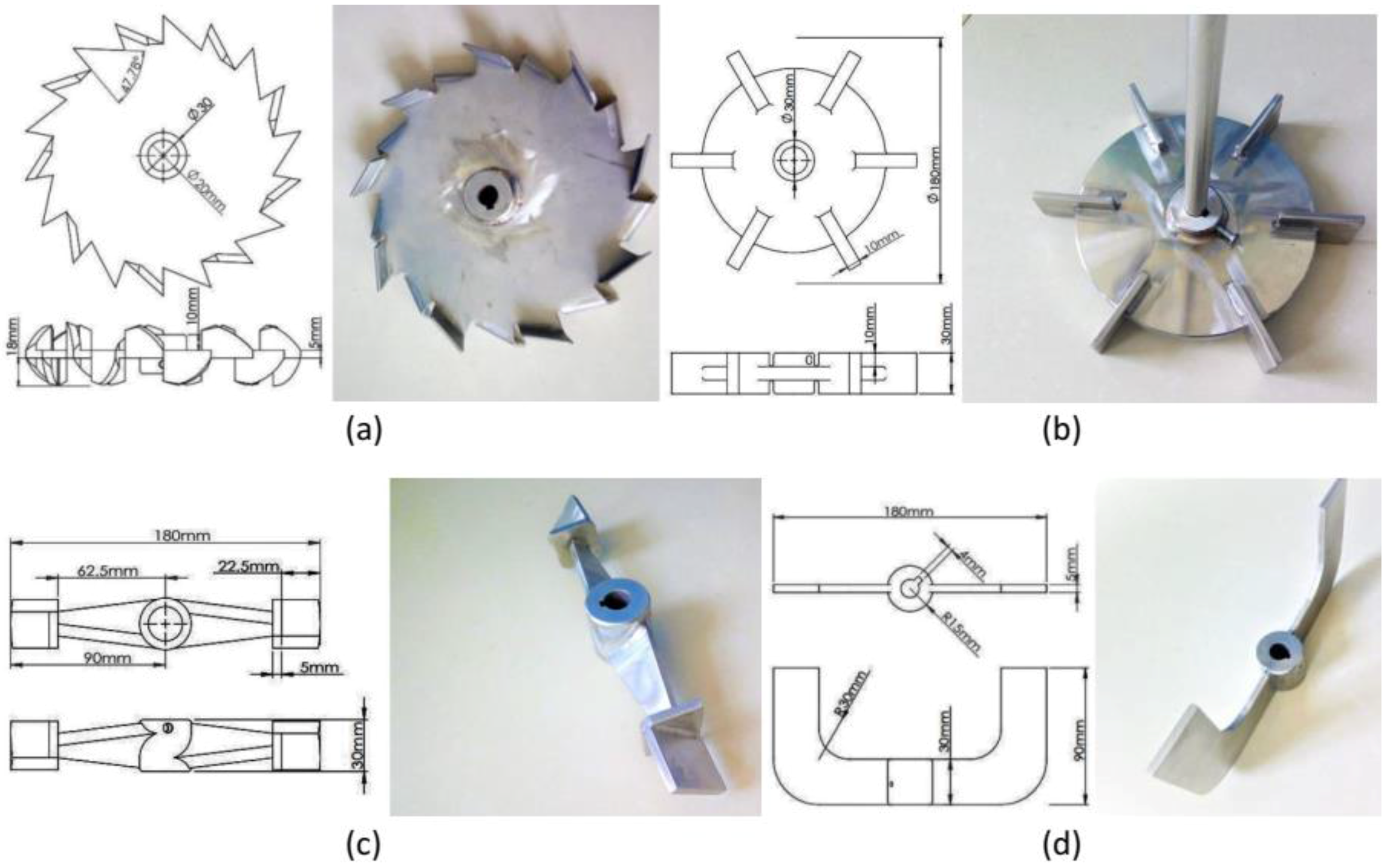
The four distinct designs of impellers used for the experiment were designed in Solid-works 2016 computer aided design (CAD) software and manufactured using Computer Numerical Machines (CNC). They were all open left-hand (LH) types and made of SUS304 steel. The blade thickness of the impellers was 2.5 mm with a diameter of 0.180 m (T/D = 0.5).
The impellers were placed 60 mm above the tangential line of the liquid bottom surface. A working angular velocity of 100 rpm was used for all the designs.
Figure 3 below shows the design details of the impellers and the manufactured experimental designs.
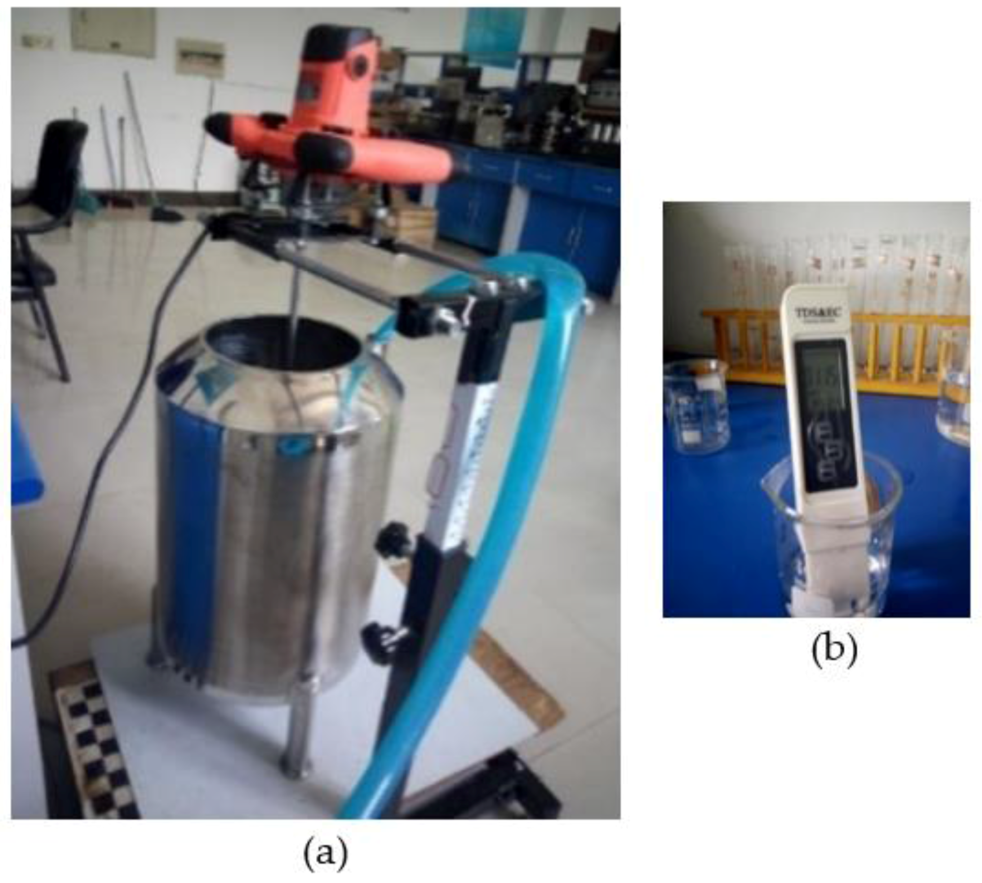
Three hundred grams of potassium sulfate granules were dissolved for a period of two minutes for each impeller construction. Eleven samples of the resultant solution were collected at different points as the solution was drained through the valve at the bottom of the tank. The points of sample collection were identified when the solution was at an interval of 50 mm (5 cm) apart along the vertical cross-section (i.e., 0 mm, 50 mm, 100 mm … 500 mm). EC values of the resultant sampled solutions were measured using an EC-meter. K2SO4 was used as the tracer element in this experiment because it dissolves and ionize readily in water [18]. Figure 4 below shows the laboratory set-up of the experimental apparatus and the Electrical conductivity meter used to measure the electrical conductivity values.
The samples tested represented the solution from the different specific regions of the tank and would be used to predict the concentration variability of the dissolved solids in the entire container.
2.2. Numerical Modeling
Simulations of the mixing process were done in CFD using an ANSYS Fluent 18.1 solver. The design model used was an agitated baffled-cylindrical vessel of identical dimensions to the one used in the experimental tests.
The aim of turbulence simulation is to predict the physical behavior of turbulent flow generated in a system using numerical methods. Turbulent motions in engineering applications are three-dimensional, non-homogenous and non-isotropic. The various methods of simulating this behavior allows for the statistical description of variable flow fields using the post-process. A modeling method used should ensure accuracy, simplicity and computational efficiency [19].
A number of approaches have been employed for turbulent flow simulation in stirred tanks. In the case of CFD, the Reynolds-averaged Navier–Stokes (RANS) equations, the Large Eddy Simulation (LES) and the Direct Numerical Simulation (DNS) are the three main methods commonly used.
In the RANS technique, the equations are averaged over a time interval or across a collection of equivalent fields. RANS computations are extensively used in practical computations for predicting steady-state solutions. Anisotropy in the nature of flow introduces a key uncertainty in the computation.
The Navier-Stokes equations are used to represent the characteristics of turbulence and form the basis of describing the flow phenomena. The chaotic nature of turbulent fluxes act as a direct result of non-linear terms in the N-S equations. These equations are based on the conservation laws namely the continuity, momentum and energy conservation laws as respectively given below [20].
where u, ρ, e and q are the velocity components, density, total energy per unit volume, and heat flux, respectively.
The stress tensor, P for a Newtonian fluid is defined by:
where, is the scalar pressure, I, is a unit diagonal tensor, T is the temperature, and μ is the dynamic viscosity coefficient.
The k-ε model is a two-equation method under the RANS approach, where, the turbulent kinetic energy (TKE) and its dissipation rate (ε) are used to describe the unsteady fields. These two parameters are obtained in the flow field by solving their modeled partial differential transport equations.
The standard k-ε model solves for high Reynolds number scenarios. This model is formulated on the assumption that the Reynolds stress is proportional to the mean velocity gradient [23,24]. The constant of proportionality is taken to be the eddy viscosity, given as:
where k is the kinetic energy, ε is the dissipation rate, and is a parameter that depends on the k-ε turbulence model.
The equation showing the TKE for three-dimensional flows can be represented as:
The governing transport equations (k-equation and ε-equation) for the Standard k-ε model are given below by Equations (8) and (9) respectively,
where is the dissipation rate time scale that characterizes the dynamic process in the energy spectrum and P is the evolution of turbulence, represented respectively as,
The values of empirical constants of the Standard k-ε model are = 0.09, = 1, = 1.314, = 1.44, and = 1.92.
The standard k-ε model combines reasonable accuracy, time economy, and robustness for a wide range of turbulent flows [25,26]. To improve the predictive accuracy of k-ε models, more transport equations have been derived. These include the realizable k-ε and the k-ε RNG (renormalization group) methods.
The realizable k-ε model contains an additional state of eddy viscosity and a transport equation for the dissipation derived from an exact equation for the transport of the mean square vorticity variations. A disadvantage of this model is that it produces non-physical turbulent viscosities in the turbulent viscosity equation. Thus, the use of this model is limited.
The k-ε RNG model is a method where the smallest eddies are first resolved in the inertial range and then represented in terms of the next smallest eddies. This process continues until a modified set of the Navier Stokes equations is obtained which can then be solved. This approach still poses modeling problems of imperfectly solved eddies.
Generally, the main weakness associated with the RANS models is that it fails to predict satisfactorily the explicit characteristics of complex flows, since the k-ε model assumes the isotropy of turbulence. Anisotropic models such as Reynolds Stress Model (RSM), DNS and the LES model have been applied in the simulation of complex three-dimensional flows.
RSM presents good accuracy in predicting flows with swirl, rotation and high strain rates. It consists of six transport equations for the Reynolds stresses and an equation for the dissipation rate, making it computationally cumbersome. This model also lacks universality in its parameters and it does not adequately capture the time dependent nature of flow.
The DNS is based on a three-dimensional and unsteady solution of the Navier-Stokes equations. However, the drawback of this model is its Reynolds number limitations, since the resolution of all the fine scales of a high Reynolds number flow requires enormous computing capability. In addition, it is hard to prove if it yields fully resolved eddies, because it would be impractical with inadequate computing ability.
LES has arisen as a possible choice for modeling, where the time-dependent behavior of the flow is resolved. It is based on the idea that the big eddies produced in the mean flow are anisotropic and have a lengthy lifespan. On the other hand, the small eddies produced from inertial transfer have more universal properties and are isotropic with a short life span hence relatively easy to model. Equations describing this model are derived by filtering the Navier–Stokes equation [27]. This effectively separates the eddies whose scales are smaller than the filter size used in meshing. The resulting equations have the structure of the original equation and resultant subgrid scale stresses (SGS). The large eddies are resolved directly, while the small eddies are modelled using available subgrid-scale models.
The filtered Navier–Stokes and conservation equation of LES for incompressible flows are as shown below:
where the items with bars indicate the large scales obtained from grid filtering.
The effects of the SGS are reflected in the subgrid scale stress tensor represented as:
The LES model can solve all eddying scales in a complex flow: however, the challenge of limited computing power still prevails, and thus not suitable for practical industrial applications. Moreover, there is excessive dissipation in flows produced by growth of initially small agitation to fully turbulent flow which ought to be resolved [28].
For these reasons, it is deemed that the RANS equations for turbulence modeling are the most fitting CFD tool to use for realistic and economical study of turbulent mixing schemes. The results obtained from the simulations using this model were an estimate prediction of the expected behavior of the impellers under study and were not fully validated in the experiments due to the scale of the computations and inadequacy of apparatus. To this effect, future work should employ reliable experimental procedures such as the laser Doppler velocimetry (LDV) or particle image velocimetry (PIV).
2.2.1. Meshing and Pre-Processing
The different impeller configurations, fluid volume, and the baffles were modelled as separate regions in Solid Works 2016 software, before being imported into ANSYS Fluent for pre-processing and meshing. Elaborate interfaces between the contacting fluid regions and boundary conditions were created in ANSYS workbench design modeler.
A mesh was generated to discretize the domains into small control volumes, where the conservation equations were to be approximated by computer numerical calculations. The mesh for the mixing simulation set-up contained two main zones, tank-fluid region, and impeller region, modelled as separate interacting fluid domains. A fine mesh was used to enhance the stability and accuracy of the computation [9].
Figure 5 below shows the boundary interfaces created and meshed regions of the agitation assembly. A compact mesh can be seen at the impeller and shaft region.
2.2.2. Simulation Set up and Computation
The simulations were prepared in fluent solver, using the pressure-based steady state and absolute velocity conditions with gravity acting in the negative y-axis direction. The created fluid regions were then set to viscous type in the k-ε standard model with standard wall functions. The material was chosen as water-liquid with a density, ρ, of 998.2 kg/m3 and constant viscosity, µ, of 0.001 kg/m.s. Cell zone conditions entailed the impeller-fluid interface, which consisted of the impeller surface and the fluid regions around the impeller. Mesh interfaces and contact regions were confirmed to be the exact points where interactions occurred.
The movement of the impeller zone in the tank-fluid region was modeled using a Multiple Reference Frame (MRF) approach that combines the computation of both stationary and moving frames. The two zones consists of well-defined boundaries. The moving zone comprised of the impeller and the shaft domains, rotating with an angular velocity of 600 rpm along the y-axis [29]. The tank-fluid zone together with the baffles and tank walls were set to the stationary frame [30].
The simulation was configured using Hybrid initialization technique before running the calculations with 200 iterations at a reporting interval of six and profile update of four cycles. The calculations were ascertained to have converged for all the computations within 1–3 h of computational time. Velocity profiles (contours, velocity streamlines and velocity vectors) were finally generated in CFD-post process to represent the effects of each impeller type. The simulations were executed using a 2.30 GHz, 4 GB RAM, (Lenovo TianYi 300-15ISK, Intel core i5) laptop computer (Lenovo Group Ltd., Beijing, China).
3. Results and Discussion
The values of electrical conductivity obtained through experiments were used to predict the mixing performance of the different impellers. CFD results were compared to the experimental data obtained on the distribution of the granules concentration in the tank.
3.1. Analysis of the Experimental Concentration Distribution
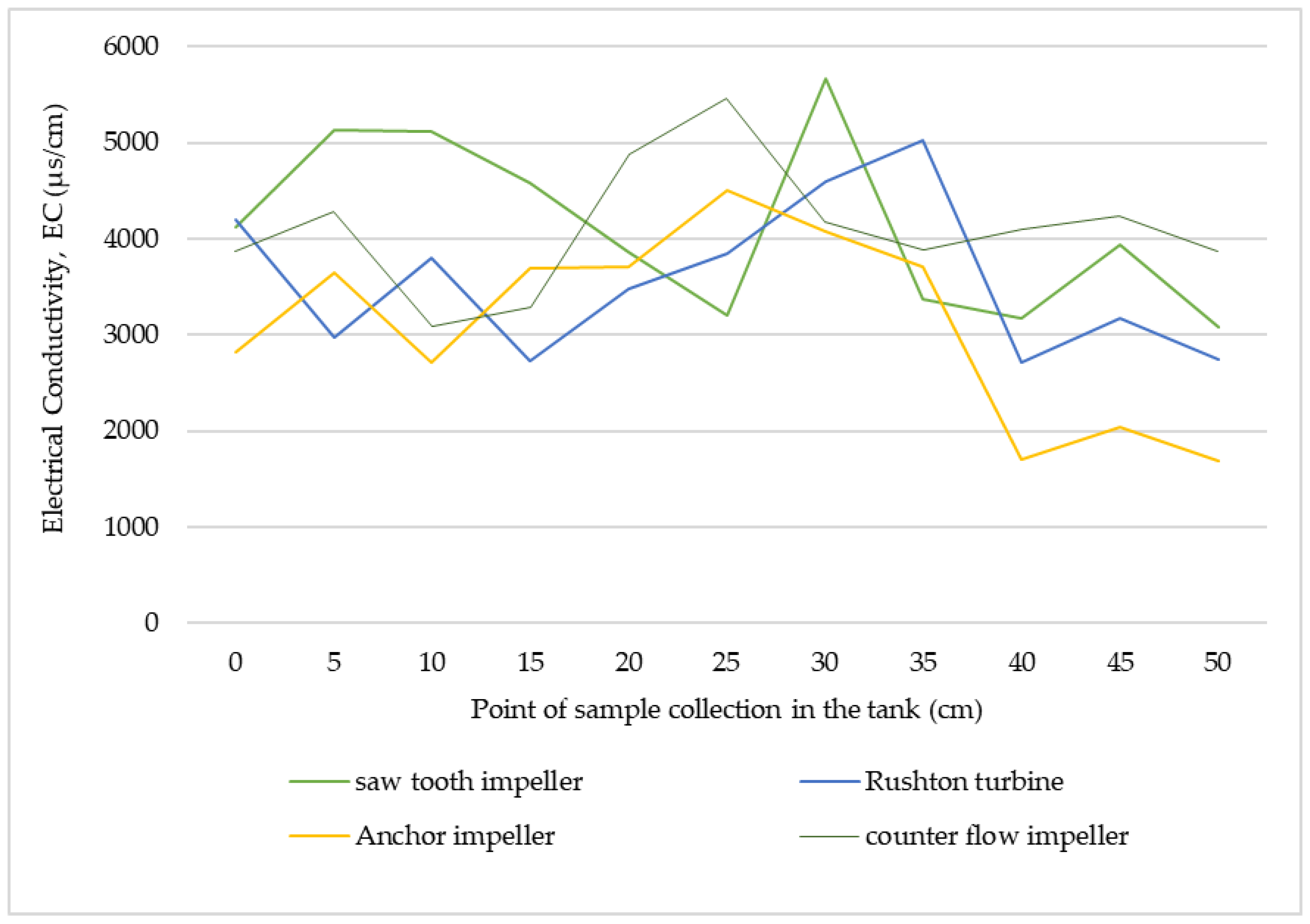
Figure 6 below shows a graphical representation of the distribution pattern of the EC values of dissolved K2SO4 in the solution. These values were assumed to be the amounts of solids at the specific regions. The horizontal axis represents the sample point in the tank from which the solution sample was collected. The vertical scale shows the values of the measured EC at the specific points. The lines show the trend of concentrations in the tank from bottom to top.
From the graph, it can be observed that the saw-tooth impeller and the counter flow impellers performed better than the anchor and the Rushton turbine in breaking down the solids into solution. The counter-flow and Rushton turbine impellers attained more uniform solution concentrations, though the mixing ability of the latter ranked lower than the former impeller.
The saw-tooth impeller was able to dissolve more granules and distribute them evenly within the solution as shown by the high values in the averages derived from the experiment (Table 2). The anchor impeller performed the least, both in the total amount of solids it dissolved and in level of homogeneity, it attained.
These results clearly point to a possibility of combining different flow patterns such as the counter-axial flow and the slots effects of the saw-tooth impellers. This will increase mixing turbulence and provide more particle interaction, which will improve the mixing performance of the impellers. Commonly used impeller types can thus be redesigned to attain better standards.
3.2. CFD Post-Process Analysis
From the numerical simulation procedures, velocity contours, streamlines and velocity vector representations were generated in CFD post process. The results represented the flow behavior of the different mixing impellers and helped in explaining the experimental outcome.
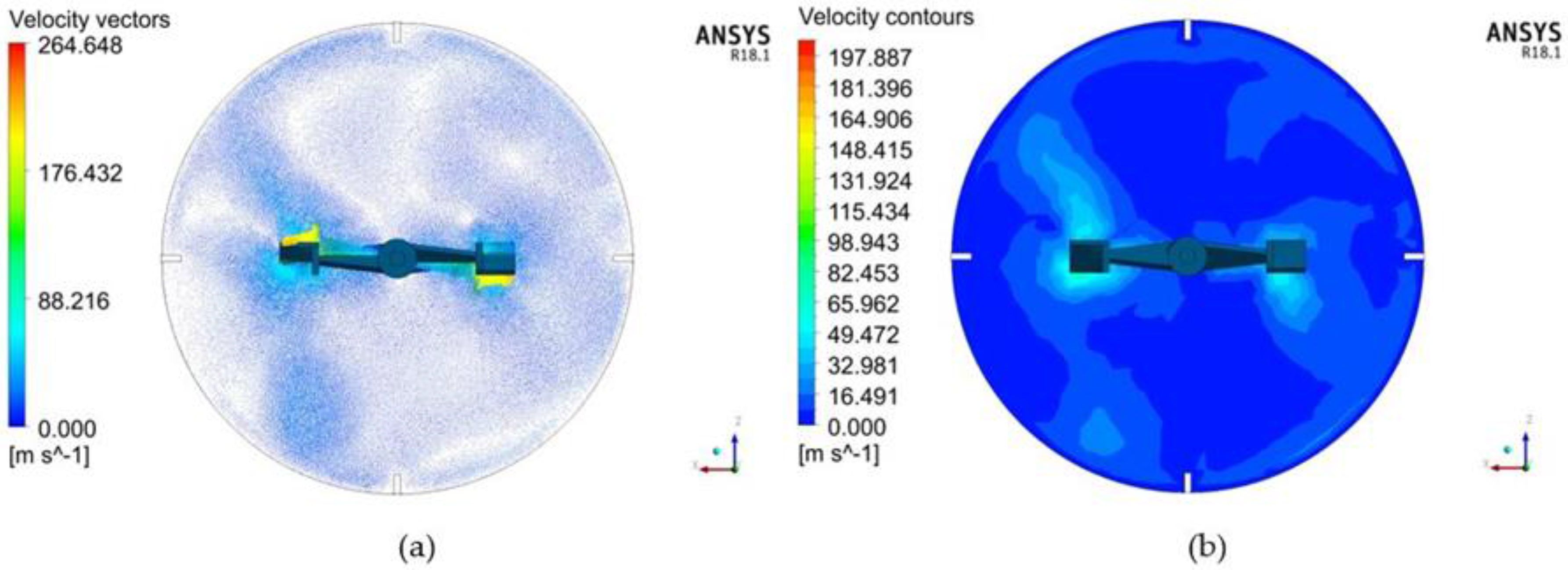
For the anchor impeller, the performance around the impeller regions was as in Figure 7 below. There was more contact between the fluid and the impeller as the impeller cut through the fluid. In the velocity vector diagram it was observed that there was a zero-flow region generated behind the blades due to the relatively wide blade cross-sectional area of this impeller.
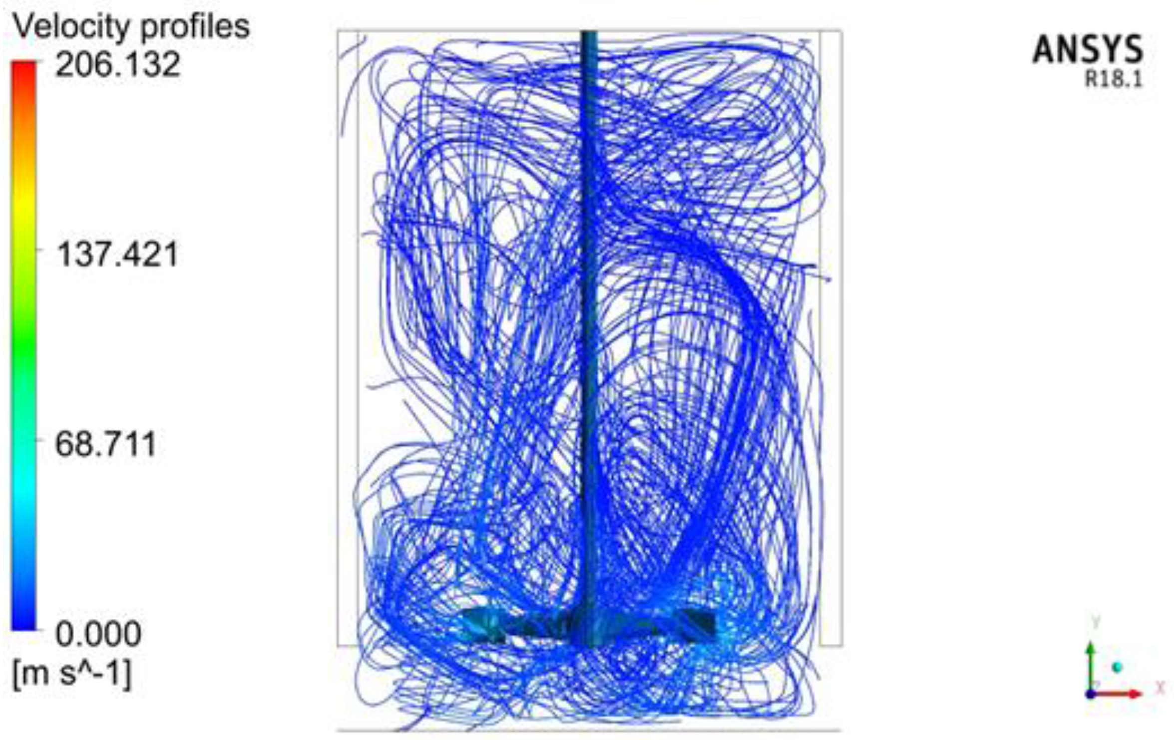
The velocity streamlines of this impeller in (Figure 8), shows that the blades drove the fluid to the walls, which then splashed back and was directed vertically and in opposite directions toward the center of the tank. There was more turbulence experienced at the impeller region, due to the large blade area. This type of impeller was not very efficient in distributing the fluid all over the tank. The generated flow is expected to cause higher concentrations of the solution in the lower parts of the tank as compared to the upper regions. This observation clearly concurs with the experimental results performed in this work as well as conclusion of Akiti, and Bai [31], who earlier proved that the anchor impeller produces less flow and turbulence regardless of the configuration of the mixing vessel.
The counter-flow impeller design is based on the idea that the blades can be modeled to produce axial flow in opposite directions. This is with the view that the counter flows generated will increase turbulence and mixing performance. From the CFD post process results, it was observed that the design was able to distribute the fluid towards the lower and upper parts of the tank efficiently. From the velocity vector contour (Figure 9), it can be seen that the fluid is well projected axially in both directions. The vector diagram shows a relatively even distribution around the impeller region.
The velocity streamlines (Figure 10), are observed to have dispersed to further regions of the tank. When mixing substances, this type of impeller will be able to efficiently distribute the particles and create a more homogenous solution.
The counter flow impeller was, thus expected to increase mixing performance due to the counter-axial flow, which improved turbulence in the vessel. This outcome agrees well with the experimental findings as well as the explanation given by McDonough [32] on the characteristics of the axial flow impellers.
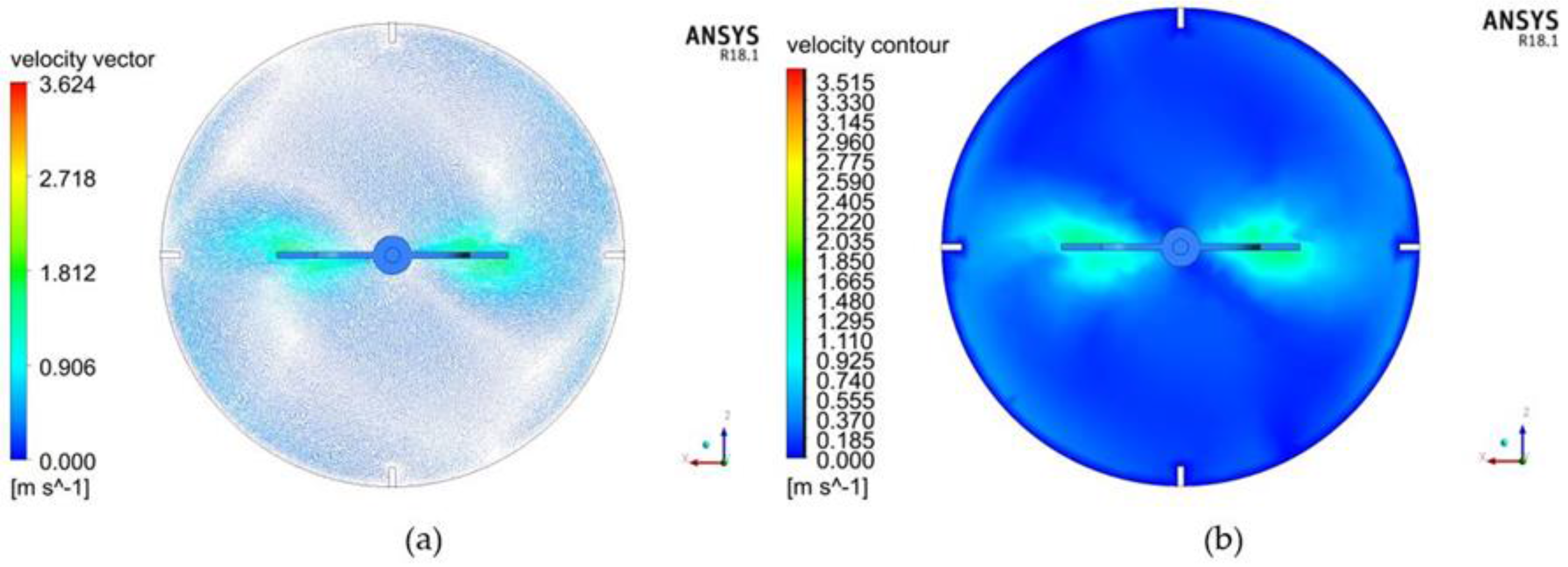
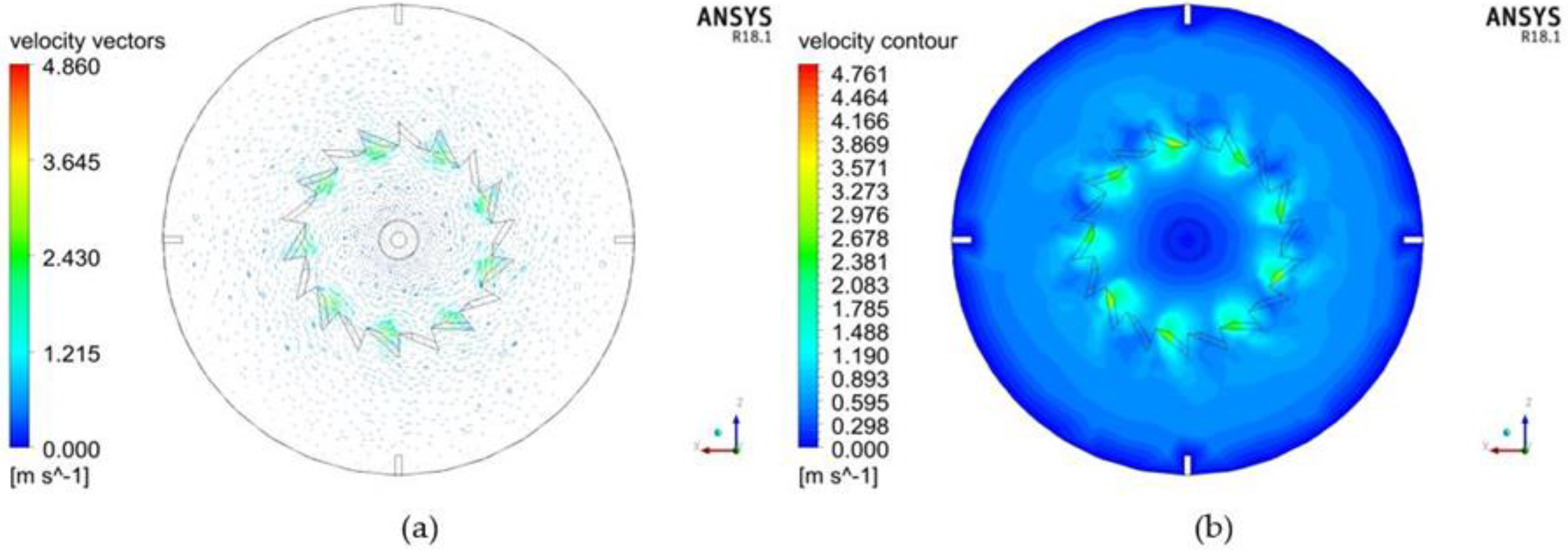
Fewer studies have been done to study the saw tooth impeller. This type of impeller uses a circular disc with protruding slots on its edges, modified to act like saw blades that cut through the fluid. Through experiments, this impeller was seen to have performed well in dissolving the solid granules. This is also proven in CFD simulation as observed in Figure 11 below. The velocity contours and vectors indicate that this impeller produced a uniform mixing result around the impeller regions as seen by the evenly distributed patterns. The slots in this disc are accredited to increasing contact area and inducing circular flow in the fluid.
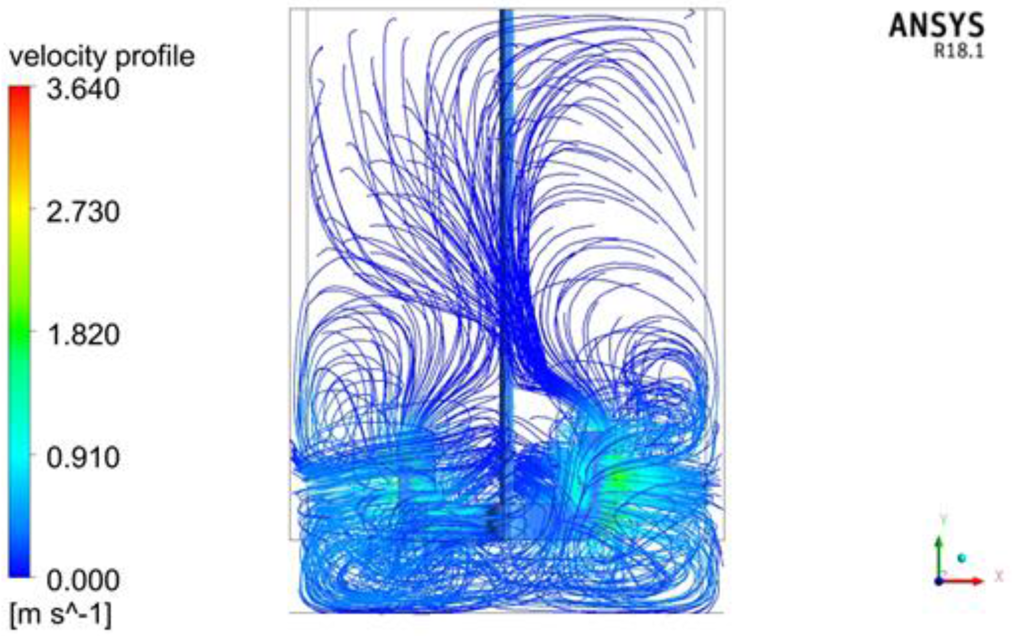
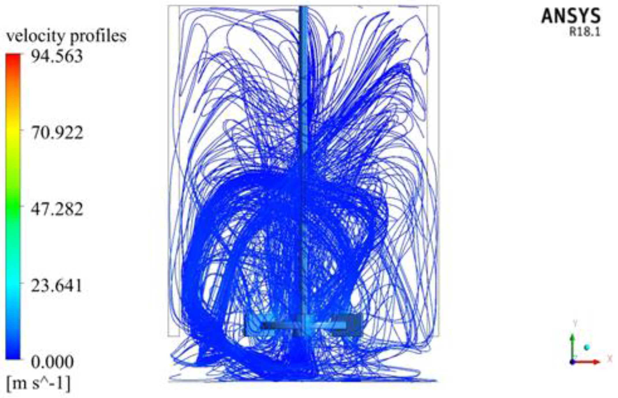
The velocity streamlines (Figure 12) shows that there was great turbulence generated as the fluid was caused to swirl in the vessel. This type of impeller was, thus expected to distribute the fluid more evenly throughout the entire volume. This validates the excellent performance of such a construction as established through experiments.
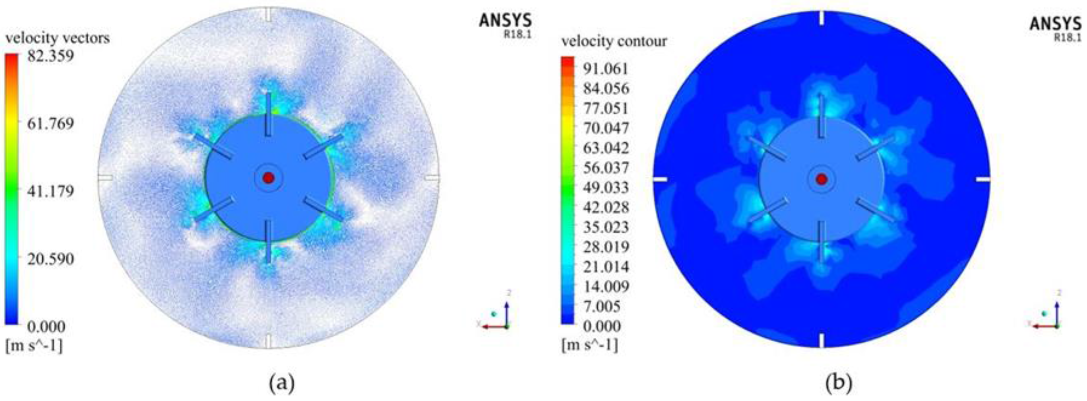
The Rushton turbine is one of the most studied agitation impellers. It has provided the basis for comparative studies for many researchers [33]. The flow patterns around the impeller region were generally well distributed due to its radial action on the fluid (Figure 13). This impeller was able to thrust the fluid from the center towards the walls of the tank and as the flow approached the wall regions, the velocity was observed to steadily drop.
The streamlines were observed (Figure 14) to move towards the wall of the stirred tank and then split into upward and downward directions. The mixing was better distributed at the central parts of the vessel as compared to the outer regions as seen from the vector diagram. The intensity of the velocity currents in the regions below the impeller was stronger than that above the impeller [34].
From the obtained results, it was evident that the unconventional impeller types (saw tooth and counter flow impellers) exhibited better mixing results, which is essential in achieving concentration homogeneity in agitation tanks. Therefore, to realize the best results from mixing processes, impellers need to be modified to generate adequate energy for creating turbulence in the vessel. Optimum designs of mixing impellers can be established by methods such as turbulent diffusivity. This method allows for numerical calculations of turbulent mixing scenarios. Turbulent diffusion is defined by a turbulent mass diffusion coefficient, Dt, which is a factor of the turbulent Schmidt number, Sct, represented as:
where, μt is the turbulent viscosity.
The Schmidt number determines the relative distribution of impeller-induced motion and mass caused by turbulence.
For efficient mixing processes, precise prediction of mixing behavior of impellers in stirred vessels is necessary. This will be beneficial when designing or selecting the most suitable apparatus. The use of the turbulence models can provide a good basis for detailed understanding of generated flow in mixing vessels. Nonetheless, the RANS, k-ε model used in this work is characterized by unsteadiness because it assumes that the flow is statistically steady [35]. This assumption leads to poor estimates for swirling and rotational flows. RANS model is valid only for fully turbulent flows, requires wall function implementation, and leads to over-prediction of turbulence in highly strained flows.
More advanced methods such as DNS model can provide better simulation results. However, they are expensive and demand immense computer capability in regards to both processor speed and capacity for storing intermediate results than in RANS methods. A more realistic alternative would be the large eddies simulation model, which has higher accuracy. It is much more economical in terms of computational power requirements than DNS. It is applicable in resolving time-dependent behavior of turbulent flow and allows computation of large and complex vortexes [36]. Like in DNS, LES have high computational cost as compared to RANS model, and is affected by viscous near-wall features.
The performance of the four impeller designs in this experiment were clearly captured by the CFD simulation model and was in good agreement with all the experimental results and prior studies conducted on the same. The good concurrence demonstrated in both the simulation and experimental procedures is an evidence that CFD is a reliable tool for explaining turbulence in mixing systems. It was also noted that numerical aspects play an important role in turbulent-flow computations in terms of both accuracy and efficiency. The future significance of CFD turbulent mixing systems will be guided by how accurate complex flows can be estimated.
For successful simulation and prediction of flow characteristics in turbulent systems, a compromise between accuracy and computing demands ought to be made. Although it was acknowledged that complex flow may not be predicted adequately with RANS models, the emphasis on simplicity, practicality, computational speed and robustness in an industrial setting influences against the adoption of more advanced models.
The ANSYS solver and numerical approach used in this work can therefore aid in the development of optimal mixing schemes in regards to the equipment geometry and related parameters. It is expected that improving the impeller designs from the conventional types will offer cheaper modes of agitation, while minimizing costs and improving on the quality of the resultant products in agricultural chemical preparations and many other fields.
4. Conclusions
The approach used in this study clearly depicted the mixing dynamics in mechanically stirred tanks, which are often difficult to predict. This technique provided relevant information about the turbulent flow characteristics. The flow patterns of the different impeller designs used in this work were satisfactorily described through experiments and CFD analysis. The results obtained from CFD simulations were confirmed to be in good agreement with experimental values. It was proven that the impeller-blade configuration significantly affected the performance of a mechanically agitated mixer. Achieving the best mixing designs will improve the quality of mixing and establish a good degree of homogeneity, as a function of the design. This work will be useful in selecting the right type of impellers that will guarantee optimum results and economical use of expensive chemicals and other mixing agents. It will also provide a basis on which large mixing systems can be designed and controlled using minimal costs, time and space.
Acknowledgments
Support from the Department of Agricultural Mechanization Engineering of Nanjing Agricultural University facilitated the successful completion of this work.
Author Contributions
Ian Torotwa conceived and designed the experiments. Changying Ji supervised the work and facilitated the acquisition and installation of the apparatus. Ian Torotwa performed and analyzed the data with extensive input from Changying Ji. Ian Torotwa wrote the paper and Changying Ji verified and approved it.
Conflicts of Interest
The authors declares no conflict of interest.
References
- Zadghaffari, R.; Moghaddas, J.S.; Revstedt, J. A Study on Liquid-Liquid Mixing in a Stirred Tank with a 6-Blade Rushton Turbine. Iran. J. Chem. Eng. 2008, 5, 12–22. [Google Scholar]
- Aubin, J.; Kresta, S.M.; Bertrand, J.; Xuereb, C.; Fletcher, D.F. Alternate Operating Methods for Improving the Performance of a Continuous Stirred Tank Reactor. Chem. Eng. Res. Des. 2006, 84, 569–582. [Google Scholar] [CrossRef] [Green Version]
- Tatterson, G.B. Fluid Mixing and Gas Dispersion in Agitated Tanks; McGraw-Hill: New York, NY, USA, 1991. [Google Scholar]
- Mak, A.T.C. Solid-Liquid Mixing in Mechanically Agitated Vessels. Ph.D. Thesis, University of London, London, UK, 1992. [Google Scholar]
- Delvigne, F.; Destain, J.; Thonart, P. Structured Mixing Model for Stirred Bioreactors: An Extension to the Stochastic Approach. Chem. Eng. J. 2005, 113, 1–12. [Google Scholar] [CrossRef]
- Raju, R.; Balachandar, S.; Hill, D.F.; Adriana, R.J. Reynolds Number Scaling of Flow in a Stirred Tank with Rushton Turbine. Part II—Eigen Decomposition of Fluctuation. Chem. Eng. Sci. 2005, 60, 3185–3198. [Google Scholar] [CrossRef]
- Isabela, M.P.; Leandro, S.O. CDF Modelling and Simulation of Transesterification Reactions of Vegetable Oils with an Alcohol in Baffled Stirred Tank Reactor. Appl. Mech. Mater. 2013, 390, 86–90. [Google Scholar]
- Seyed, H.; Dineshkumar, P.; Farhad, E.M.; Mehrab, M. Study of Solid-Liquid Mixing in Agitated Tanks through Computational Fluid Dynamics Modeling. Ind. Eng. Chem. Res. 2010, 49, 4426–4435. [Google Scholar]
- Versteeg, H.K.; Malalasekera, W. An Introduction to Computational Fluid Dynamics. In The Finite Volume Method, 2nd ed.; Pearson Education: New York, NY, USA, 2007. [Google Scholar]
- Zhang, Z.; Liu, H.; Zhu, S.P.; Zhao, F. Application of CFD in ship engineering design practice and ship hydrodynamics. J. Hydrodyn. 2006, 18, 315–322. [Google Scholar] [CrossRef]
- Zlokarnik, M. Scale-Up in Chemical Engineering, 2nd ed.; Wiley-VCH: Weinheim, Germany, 2006. [Google Scholar]
- Pakzad, L.; Ein-Mozaffari, F.; Chan, P. Using computational fluid dynamics modeling to study the mixing of pseudoplastic fluids with a Scaba 6SRGT impeller. Chem. Eng. Process. 2008, 47, 2218–2227. [Google Scholar] [CrossRef]
- Ge, C.-Y.; Wang, J.-J.; Gu, X.-P.; Feng, L.-F. CFD simulation and PIV measurement of the flow field generated by modified pitched blade turbine impellers. Chem. Eng. Res. Des. 2014, 92, 1027–1036. [Google Scholar] [CrossRef]
- Cokljat, D.; Slack, M.; Vasquez, S.A.; Bakker, A.; Montante, G. Reynolds-Stress Model for Eulerian Multiphase. Prog. Comput. Fluid Dyn. 2006, 6, 168–178. [Google Scholar] [CrossRef]
- Khopkar, A.R.; Kasat, G.R.; Pandit, A.B.; Ranade, V.V. Computational Fluid Dynamics Simulation of the Solid Suspension in a Stirred Slurry Reactor. Ind. Eng. Chem. Res. 2006, 45, 4416–4428. [Google Scholar] [CrossRef]
- Zalc, J.M.; Szalai, E.S.; Alvarez, M.M.; Muzzio, F.J. Using CFD to understand chaotic mixing in laminar stirred tanks. AIChE J. 2002, 48, 2124–2134. [Google Scholar] [CrossRef]
- Tatterson, G.B. Scale-Up and Design of Industrial Mixing Processes; McGraw-Hill: New York, NY, USA, 1994. [Google Scholar]
- Jiusheng, L.; Yibin, M.; Bei, L. Field evaluation of fertigation uniformity as affected by injector type and manufacturing variability of emitters. Irrig. Sci. 2007, 25, 117–125. [Google Scholar]
- Leschziner, M.A.; Drikakis, D. Turbulence and turbulent flow computation in aeronautics. Aeronaut. J. 2002, 106, 349–384. [Google Scholar]
- ANSYS Fluent User Guide. Available online: http://www.ansys.fem.ir/ansys_fluent (accessed on 12 November 2017).
- Paul, E.L.; Atiemo-Obeng, V.A.; Kresta, S.M. Handbook of Industrial Mixing: Science and Practice; Wiley-Interscience: New York, NY, USA, 2004. [Google Scholar]
- Dagadu, C.P.K.; Stegowsk, Z.; Furman, L.; Akaho, E.H.K.; Danso, K.A. Determination of Flow Structure in a Gold Leaching Tank by CFD Simulation. J. Appl. Math. Phys. 2014, 2, 510–519. [Google Scholar] [CrossRef]
- Launder, B.E.; Spalding, D.B. The Numerical Computation of Turbulent Flows. Comput. Meth. Appl. Mech. Eng. 1974, 3, 269–289. [Google Scholar] [CrossRef]
- Kresta, S.M.; Wood, P.E. Prediction of the Three-Dimensional Turbulent Flow in Stirred Tanks. AIChE J. 1991, 37, 448–460. [Google Scholar] [CrossRef]
- Barrue, H.; Bertrand, J.; Cristol, B.; Xuereb, C. Eulerian Simulation of Dense Solid-Liquid Suspension in Multi-Stage Stirred Vessel. J. Chem. Eng. Jpn. 2001, 34, 585–594. [Google Scholar] [CrossRef]
- Oshinowo, L.M.; Bakker, A. CFD Modeling of solids Suspensions in Stirred Tanks. Presented at the Symposium on Computational Modeling of Metals, Minerals and Materials, TMS Annual Meeting, Seattle, WA, USA, 17–21 February 2002. [Google Scholar]
- Leonard, A. Energy cascade in large-eddy simulations of turbulent fluid flow. Adv. Geophys. 1974, 18, 237–248. [Google Scholar]
- Pope, S. Turbulent Flows; Cambridge University Press: Cambridge, UK, 2000. [Google Scholar]
- Luo, J.Y.; Issa, R.I.; Gosman, A.D. Prediction of Impeller Induced Flows in Mixing Vessels Using Multiple Frames of Reference. Inst. Chem. Eng. Symp. Ser. 1994, 136, 549–556. [Google Scholar]
- Khopkar, A.R.; Mavros, P.; Ranade, V.V.; Bertrand, J. Simulation of Flow Generated by an Axial Flow Impeller: Batch and Continuous Operation. Chem. Eng. Res. Des. 2004, 82, 737–751. [Google Scholar] [CrossRef]
- Akiti, O.; Yeboah, A.; Bai, G. Hydrodynamic effects on mixing and competitive reactions in laboratory reactors. Chem. Eng. Sci. 2005, 60, 2341–2354. [Google Scholar] [CrossRef]
- McDonough, R.J. Mixing for the Process Industries; Van Nostrand Reinhold: New York, NY, USA, 1992. [Google Scholar]
- Musgrove, M.; Ruszkowski, S.; Van den Akker, H.; Derksen, J. Influence of impeller type and agitation conditions on the drop size of immiscible liquid dispersions. In Proceedings of the 10th European Conference on Mixing, Delft, The Netherlands, 2–5 July 2000; Elsevier Science: Amsterdam, The Netherlands, 2000; pp. 165–172. [Google Scholar]
- Divyamaan, W.; Ranjeet, P.U.; Moses, O.T.; Vishnu, K.P. CFD simulation of solid-liquid stirred tanks. Adv. Powder Technol. 2012, 23, 445–453. [Google Scholar]
- Drikakis, D. Advances in turbulent flow computations using high-resolution methods. Prog. Aerosp. Sci. 2003, 39, 405–424. [Google Scholar] [CrossRef]
- Som, S.; Senecal, P.K.; Pomraning, E. Comparison of RANS and LES Turbulence Models against Constant Volume Diesel Experiments. In Proceedings of the 24th Annual Conference on Liquid Atomization and Spray Systems (ILASS Americas), San Antonio, TX, USA, 20–23 May 2012. [Google Scholar]
Figure 1.
Experimental apparatus set-up showing the assembly that was used to perform the mixing experiment.
Figure 1.
Experimental apparatus set-up showing the assembly that was used to perform the mixing experiment.

Figure 2.
Diagram representing the experimental set-up dimensions.

Figure 3.
Experimental impeller designs and the actual impellers tested: (a) saw-tooth impeller (b) Rushton turbine (c) counter-flow impeller and (d) anchor impeller.
Figure 3.
Experimental impeller designs and the actual impellers tested: (a) saw-tooth impeller (b) Rushton turbine (c) counter-flow impeller and (d) anchor impeller.

Figure 4.
(a) The laboratory apparatus set-up showing the mixer connected to a power source, tank filled with water, stand and a shaft connecting the motor to the impeller inside the tank. (b) Measuring electrical conductivity (EC) using an EC-meter.
Figure 4.
(a) The laboratory apparatus set-up showing the mixer connected to a power source, tank filled with water, stand and a shaft connecting the motor to the impeller inside the tank. (b) Measuring electrical conductivity (EC) using an EC-meter.

Figure 5.
(a) Boundary conditions between impeller and fluid interfaces set in ANSYS workbench design modeler; (b) Sectional view of the meshed model showing the impeller and shaft region at the center; and (c) Meshing the fluid volume.
Figure 5.
(a) Boundary conditions between impeller and fluid interfaces set in ANSYS workbench design modeler; (b) Sectional view of the meshed model showing the impeller and shaft region at the center; and (c) Meshing the fluid volume.

Figure 6.
Graph comparing the performance of the different impellers under study (Anchor, Rushton turbine, Saw-tooth and Counter-flow impellers). The lines show the trend of the dissolved solids (EC values) within the vessel. This represents the amounts of solid granules that were broken down into solution and distributed by the turbulence generated by the impeller action.

Figure 7.
Diagrams showing the (a) velocity vectors and (b) contours generated by anchor impeller.

Figure 8.
Velocity streamlines generated by the anchor impeller. More turbulence can be observed at the lower regions than the upper regions of the tank.
Figure 8.
Velocity streamlines generated by the anchor impeller. More turbulence can be observed at the lower regions than the upper regions of the tank.

Figure 9.
(a) Velocity vectors and (b) velocity contours of counter-flow impeller. More particles are seen on the axial blade surface as they are projected vertically.
Figure 9.
(a) Velocity vectors and (b) velocity contours of counter-flow impeller. More particles are seen on the axial blade surface as they are projected vertically.

Figure 10.
Flow streamlines of counter-flow impeller.

Figure 11.
(a) Velocity vectors and (b) velocity contours of saw-tooth impeller. Uniform patterns can be seen around the impeller.
Figure 11.
(a) Velocity vectors and (b) velocity contours of saw-tooth impeller. Uniform patterns can be seen around the impeller.

Figure 12.
Velocity streamlines of the saw-tooth impeller showing the swirling motion of the impeller, which is spread throughout the vessel.
Figure 12.
Velocity streamlines of the saw-tooth impeller showing the swirling motion of the impeller, which is spread throughout the vessel.

Figure 13.
(a) Velocity vectors and (b) velocity contours of Rushton turbine. The radial action of the impeller on the fluid can be observed at the blades.
Figure 13.
(a) Velocity vectors and (b) velocity contours of Rushton turbine. The radial action of the impeller on the fluid can be observed at the blades.

Figure 14.
Velocity streamlines of Rushton turbine.


Table 1.
Dimensions of the agitation apparatus.
| Parameter | Symbol | Value (mm) |
|---|---|---|
| Tank diameter | T | 360 |
| Tank height | H | 500 |
| Impeller diameter | D = T/2 | 180 |
| Impeller blade height | h | 10 |
| Baffle length | L | 440 |
| Baffle width | B = D/12 | 15 |
| Impeller clearance | C = D/3 | 60 |
Table 2.
Mean values of the measured Electrical Conductivity (EC).
| Type of Impeller | Mean EC |
|---|---|
| saw tooth impeller | 4113.5 |
| Rushton turbine | 3571.4 |
| Anchor impeller | 3119.0 |
| counter flow impeller | 4101.9 |
© 2018 by the authors. Licensee MDPI, Basel, Switzerland. This article is an open access article distributed under the terms and conditions of the Creative Commons Attribution (CC BY) license (http://creativecommons.org/licenses/by/4.0/).
Share and Cite
MDPI and ACS Style
Torotwa, I.; Ji, C. A Study of the Mixing Performance of Different Impeller Designs in Stirred Vessels Using Computational Fluid Dynamics. Designs 2018, 2, 10. https://0-doi-org.brum.beds.ac.uk/10.3390/designs2010010
AMA Style
Torotwa I, Ji C. A Study of the Mixing Performance of Different Impeller Designs in Stirred Vessels Using Computational Fluid Dynamics. Designs. 2018; 2(1):10. https://0-doi-org.brum.beds.ac.uk/10.3390/designs2010010
Chicago/Turabian StyleTorotwa, Ian, and Changying Ji. 2018. "A Study of the Mixing Performance of Different Impeller Designs in Stirred Vessels Using Computational Fluid Dynamics" Designs 2, no. 1: 10. https://0-doi-org.brum.beds.ac.uk/10.3390/designs2010010