A Novel Deep Learning Backstepping Controller-Based Digital Twins Technology for Pitch Angle Control of Variable Speed Wind Turbine

 ,
,
Abstract
:1. Introduction and Preliminaries
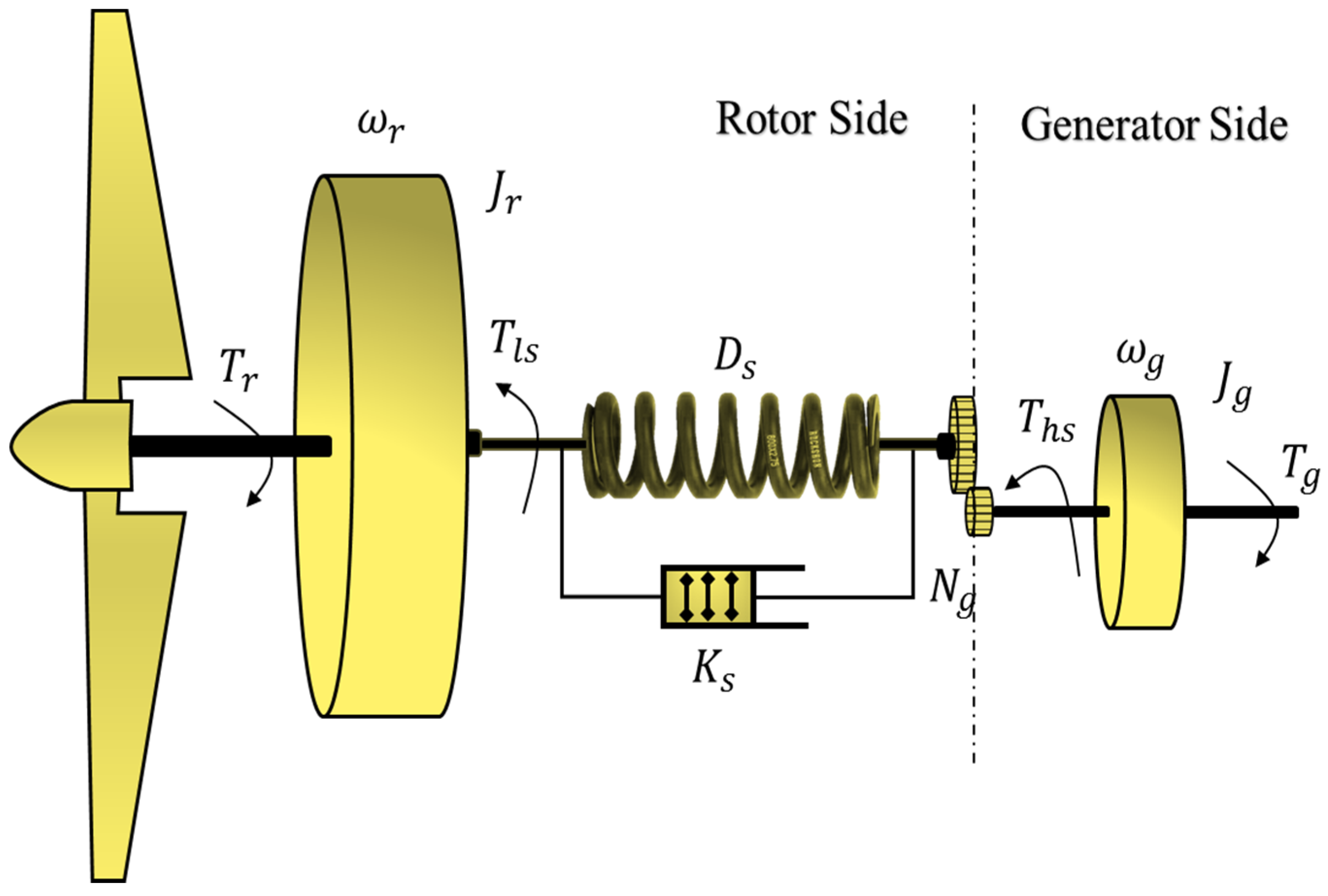
2. Variable Speed Wind Turbine Nonlinear Model
3. Design of Proposed Controller
3.1. Nonlinear Integral Backstepping Model-Free Control (NIB-MFC)
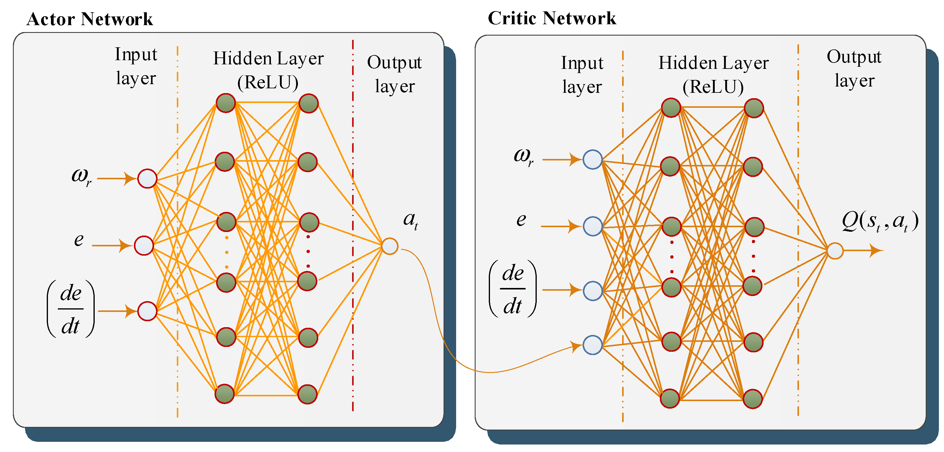
3.2. Reinforcement Learning
3.3. The Learning Process
- Markov decision process (MDP): It is the form in which the RL environment is typically stated, and it is because many RL algorithms for this context utilize dynamic programming techniques.
- Agent: The agent receives rewards by performing correctly and penalties for performing incorrectly. The agent learns without intervention from a human, by maximizing its reward and minimizing its penalty.
- Environment: The environment is the physical world in which the agent operates. The agent’s current state and action are considered as its input, and the agent’s reward and its next state are its output.
- State: State is the current situation of the agent in the environment, and is the set of all possible states of the agent.
- Policy: Policy π is the method by which the agent’s state is mapped to an appropriate action leading to the highest reward.
- Action: is the set of all possible moves that the agent can make.
- Reward: This value is the feedback from the environment as an evaluation criterion that determines the success or failure of an agent’s actions in a given state.
- Value function: The value function is defined as the long term expected to return with a discount. The discount factor () dampens the rewards’ effect on the agent’s choice of action to make future rewards worth less than immediate rewards. Roughly speaking, the value function estimates “how good” it is to be in a given state.
- Q-value: Q-value or action value is used to measure how effective taking an action at a state is.
4. Digital Twin Controller of WT System
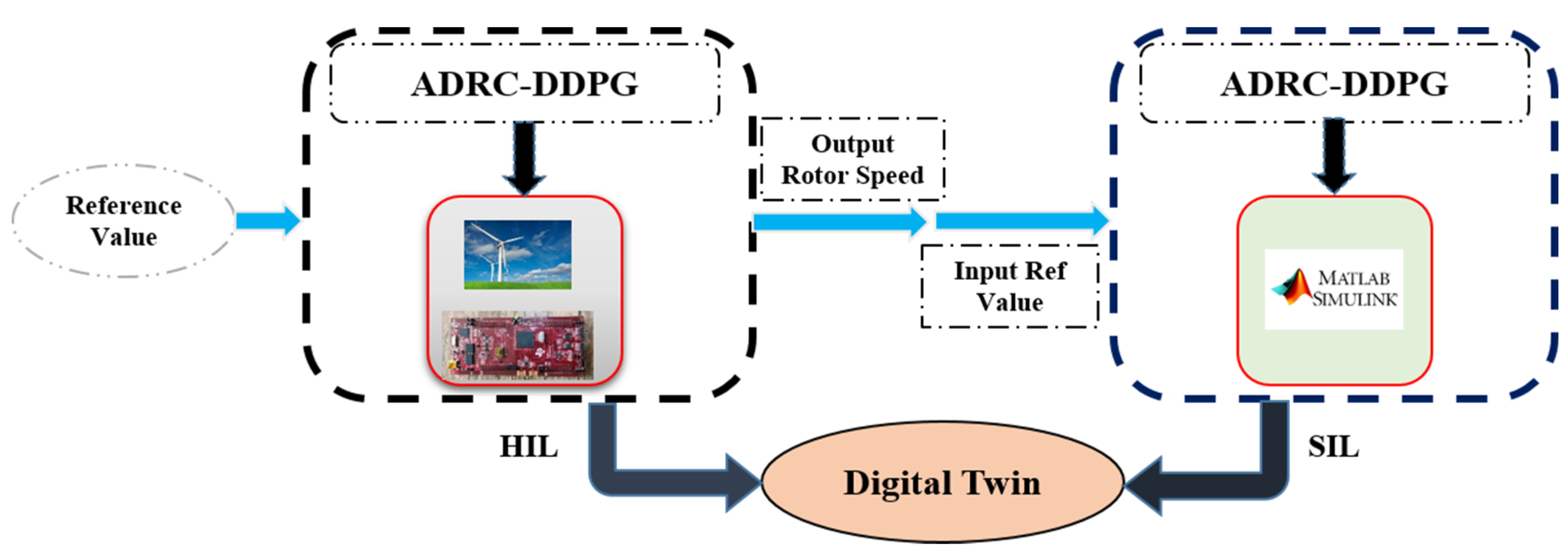
4.1. The Concept of Digital Twin
- Define the system and simulation of closed-loop control in software;
- Implementation of the proposed controller on a TI microcontroller board;
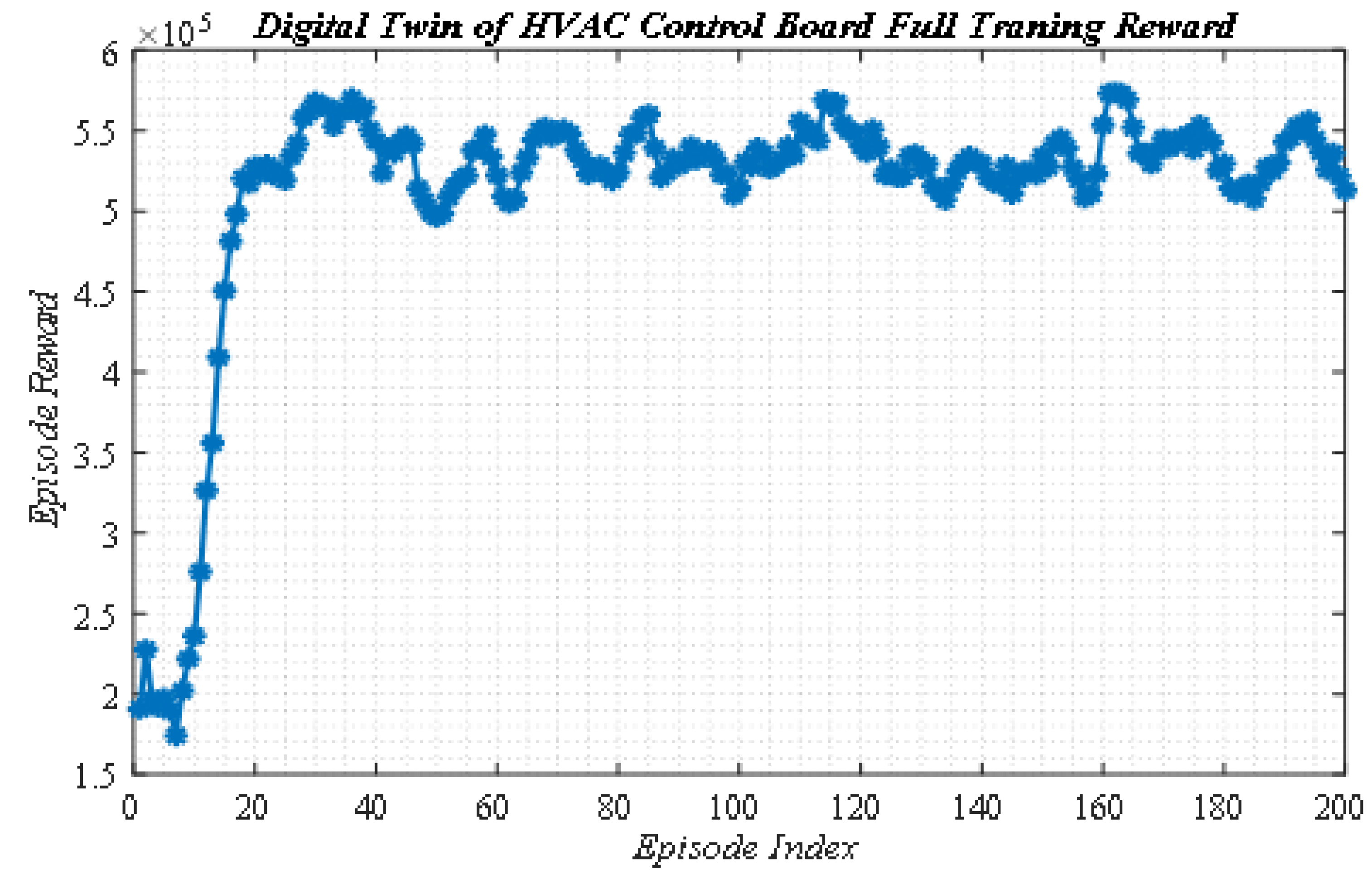
- Upgrade the controller coefficients and achieving the desired output using the DDPG-NIB method in HIL mode with real-time data;
- Optimization of control coefficients of SIL controller reusing NIB-DDPG method (criteria: similarity of SIL and HIL outputs).
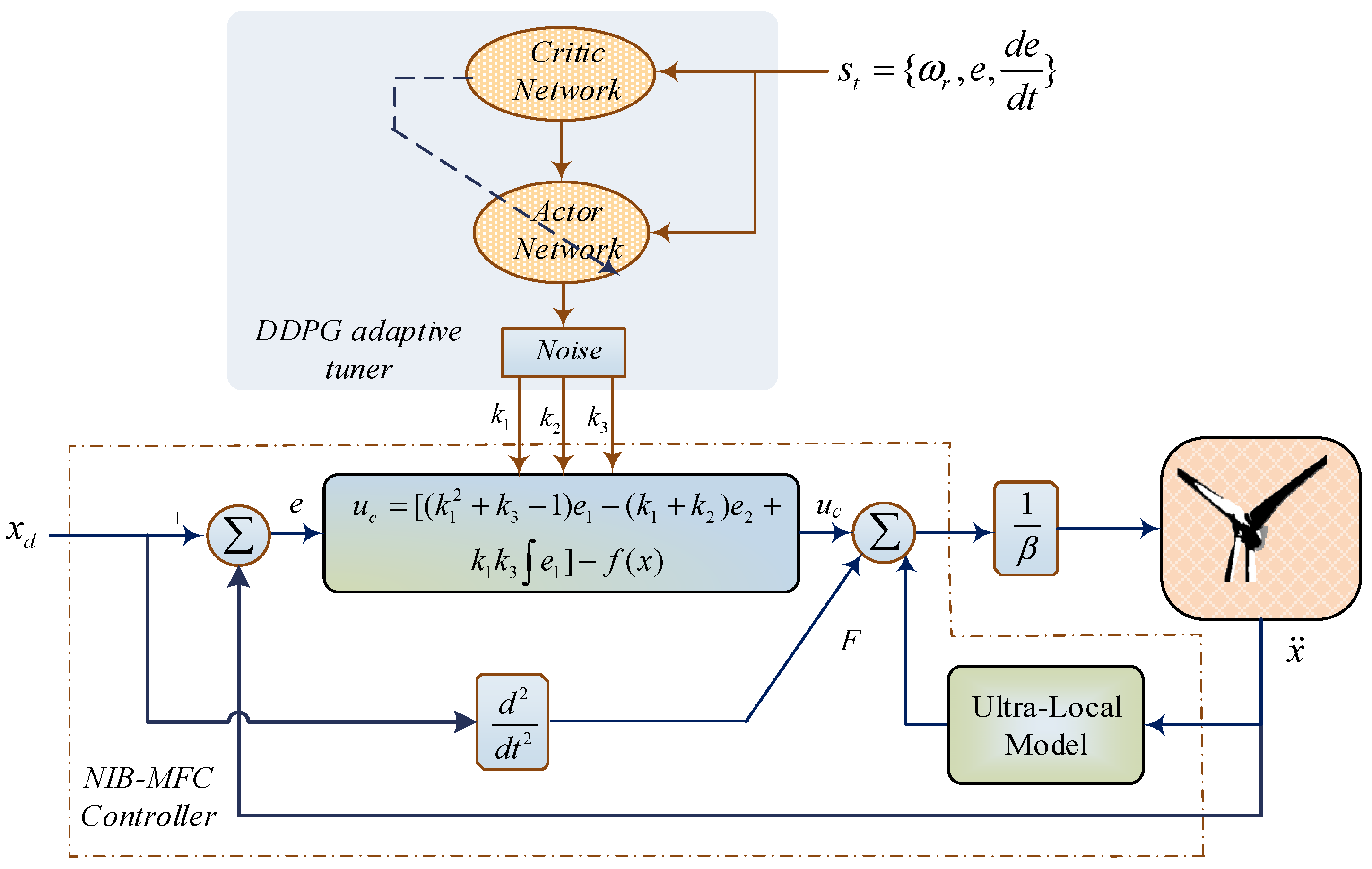
4.2. The Proposed DDPG Tuned Backstepping Control Method
4.3. Implementing the Adaptive NIB Controller Based DDPG
5. Results
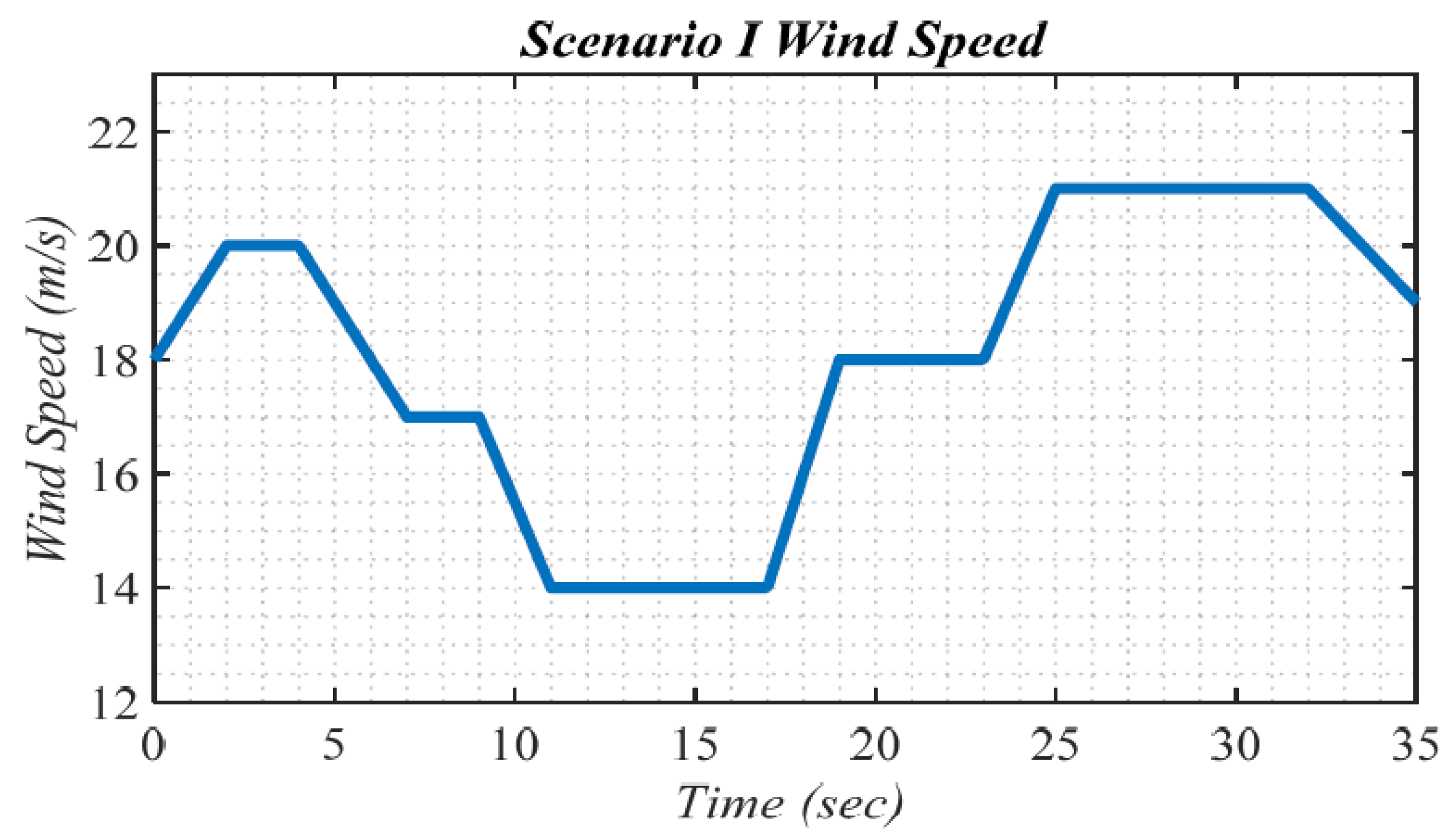
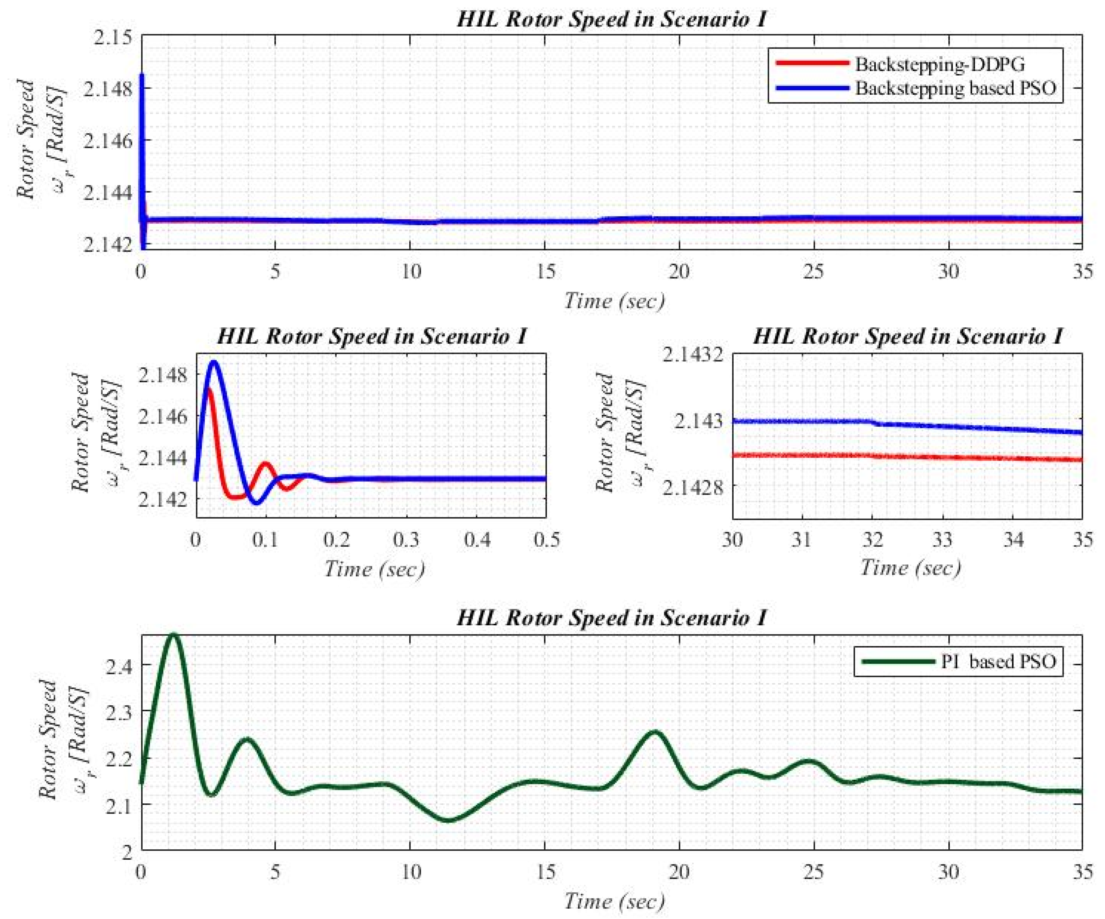
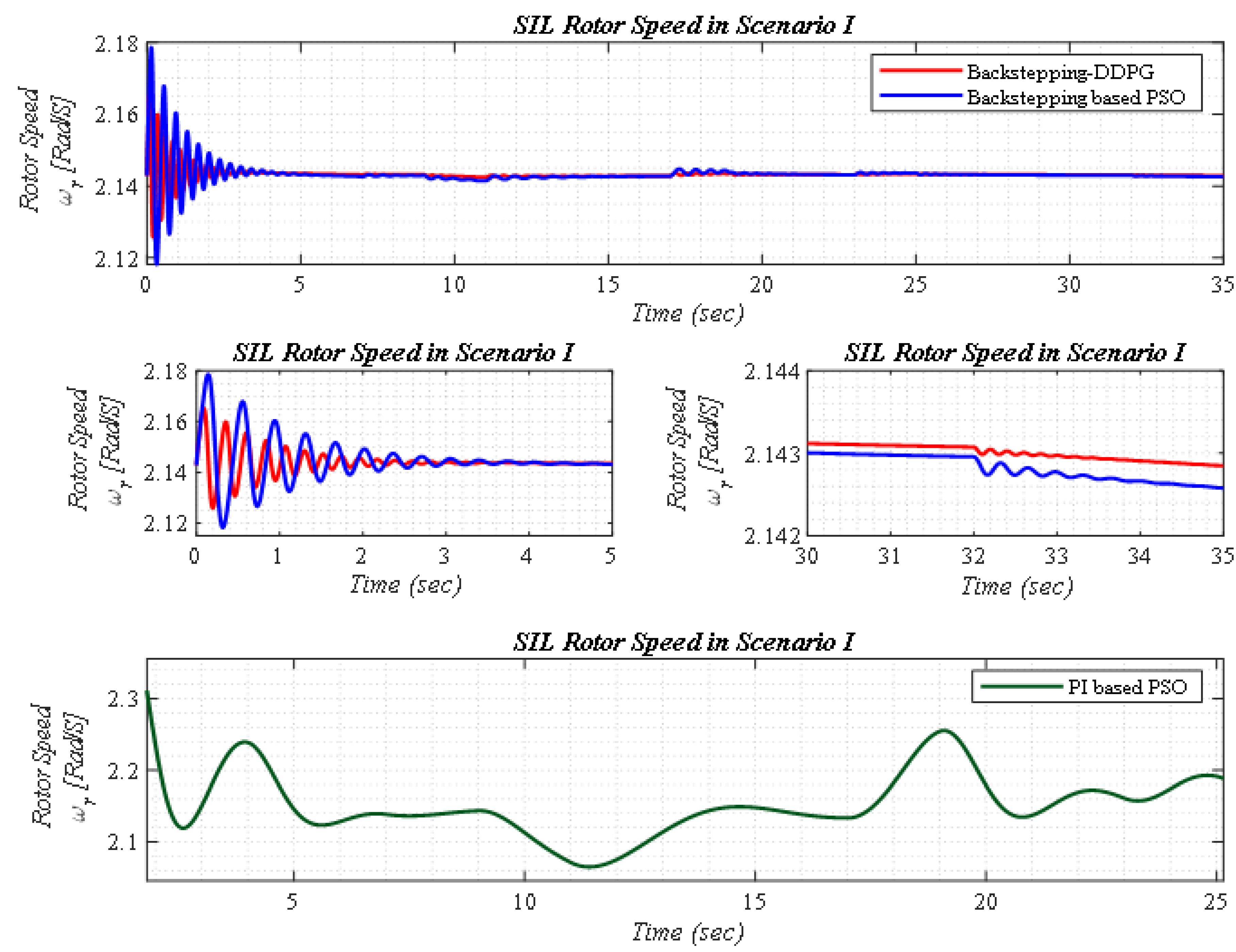
5.1. Scenario I
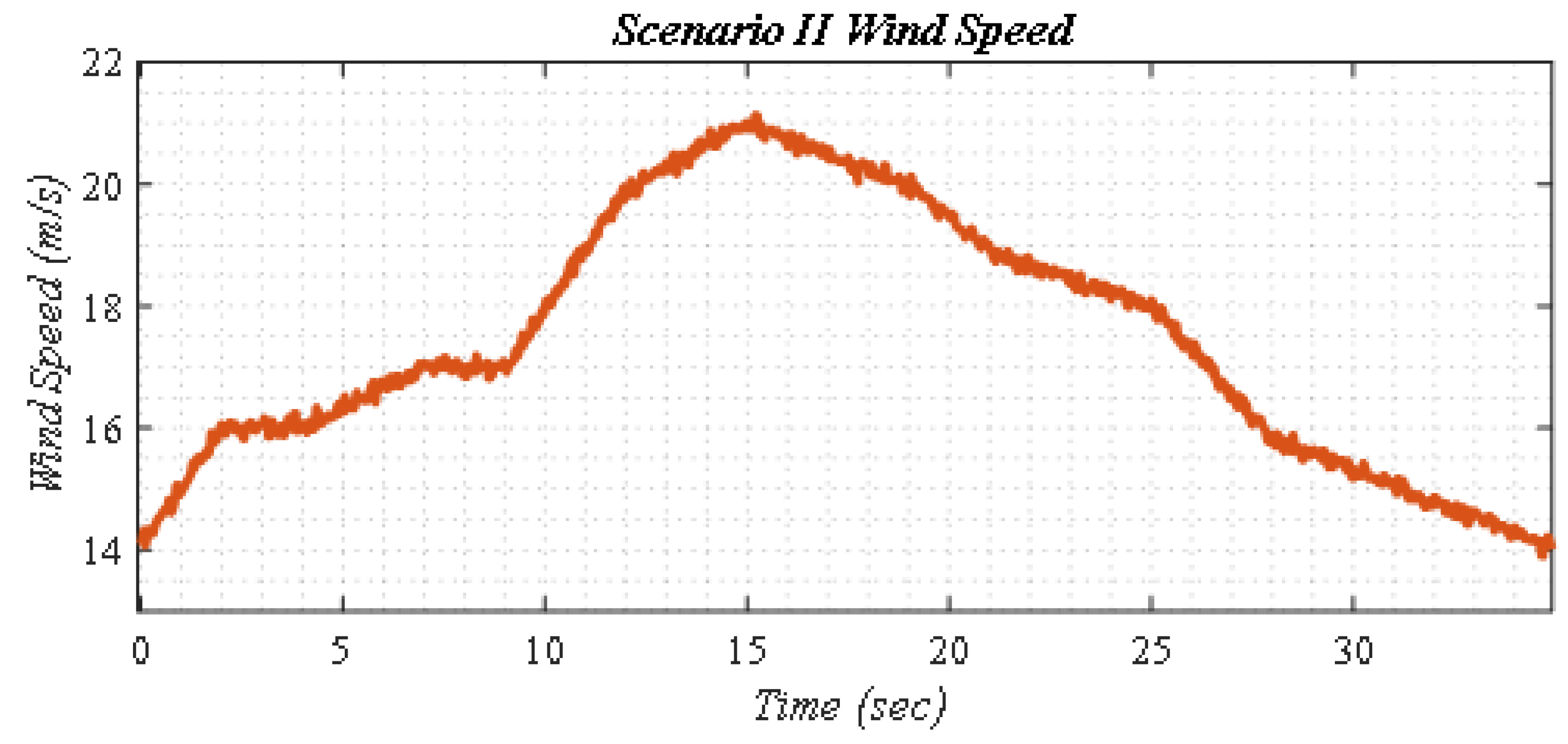
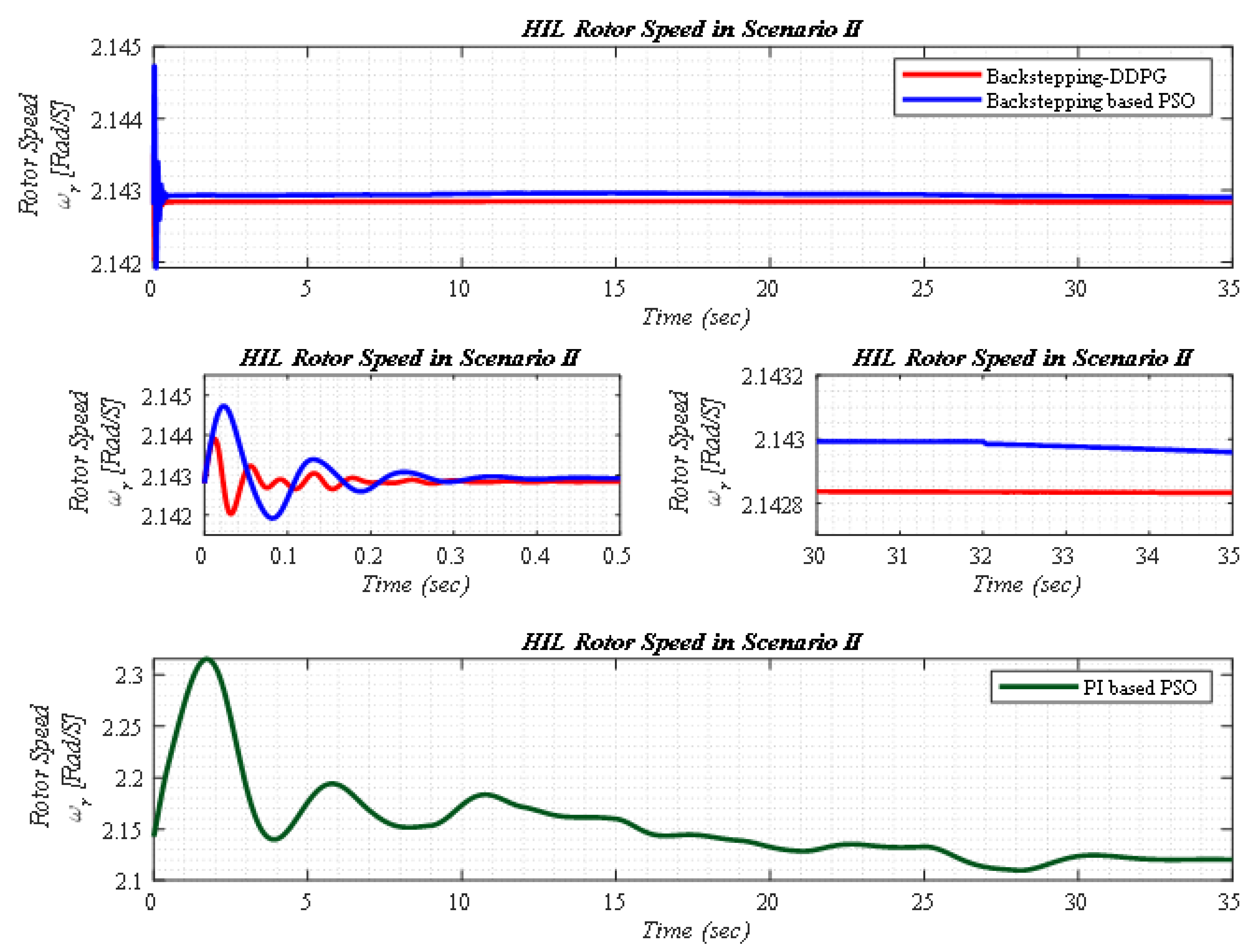
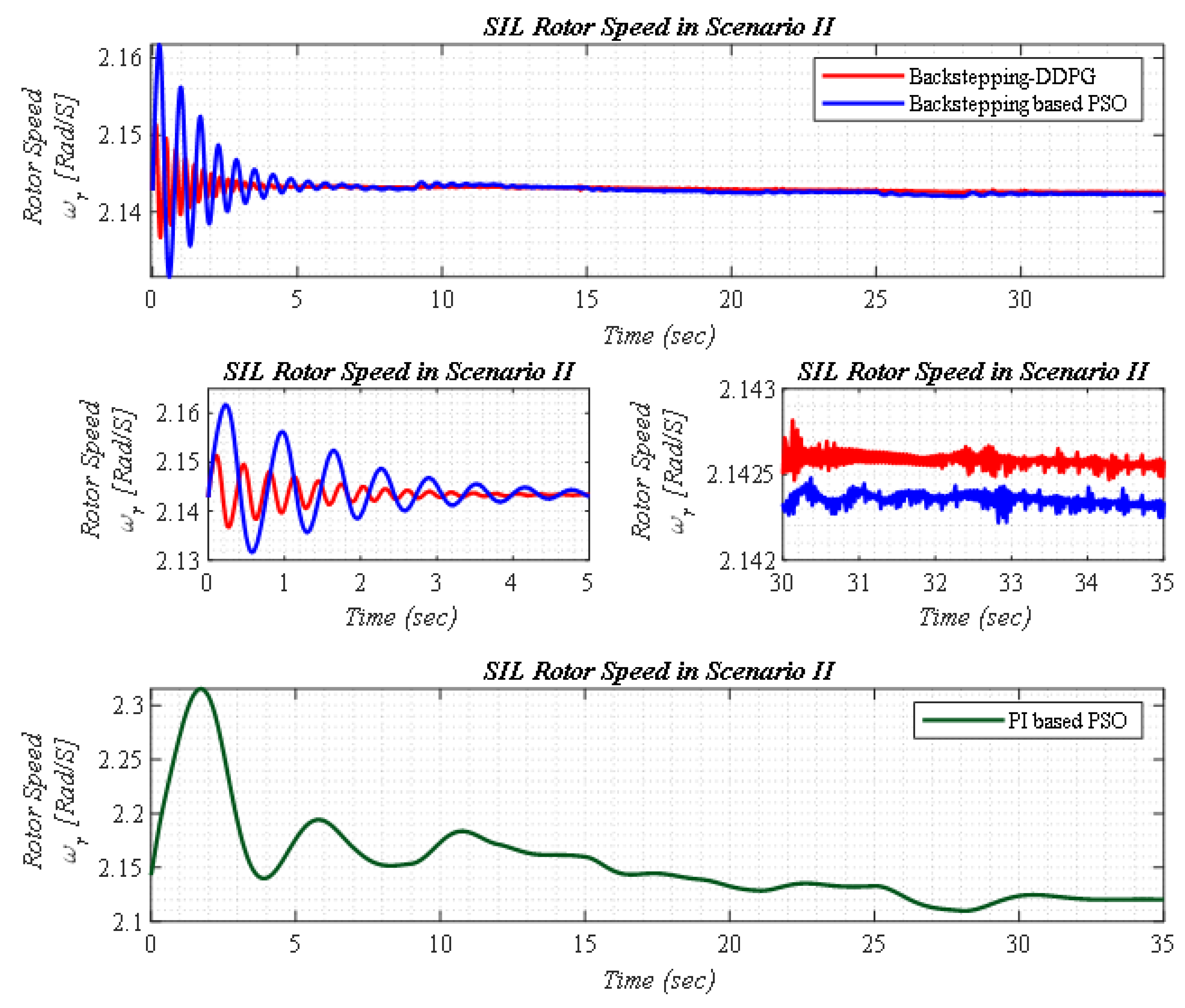
5.2. Scenario II
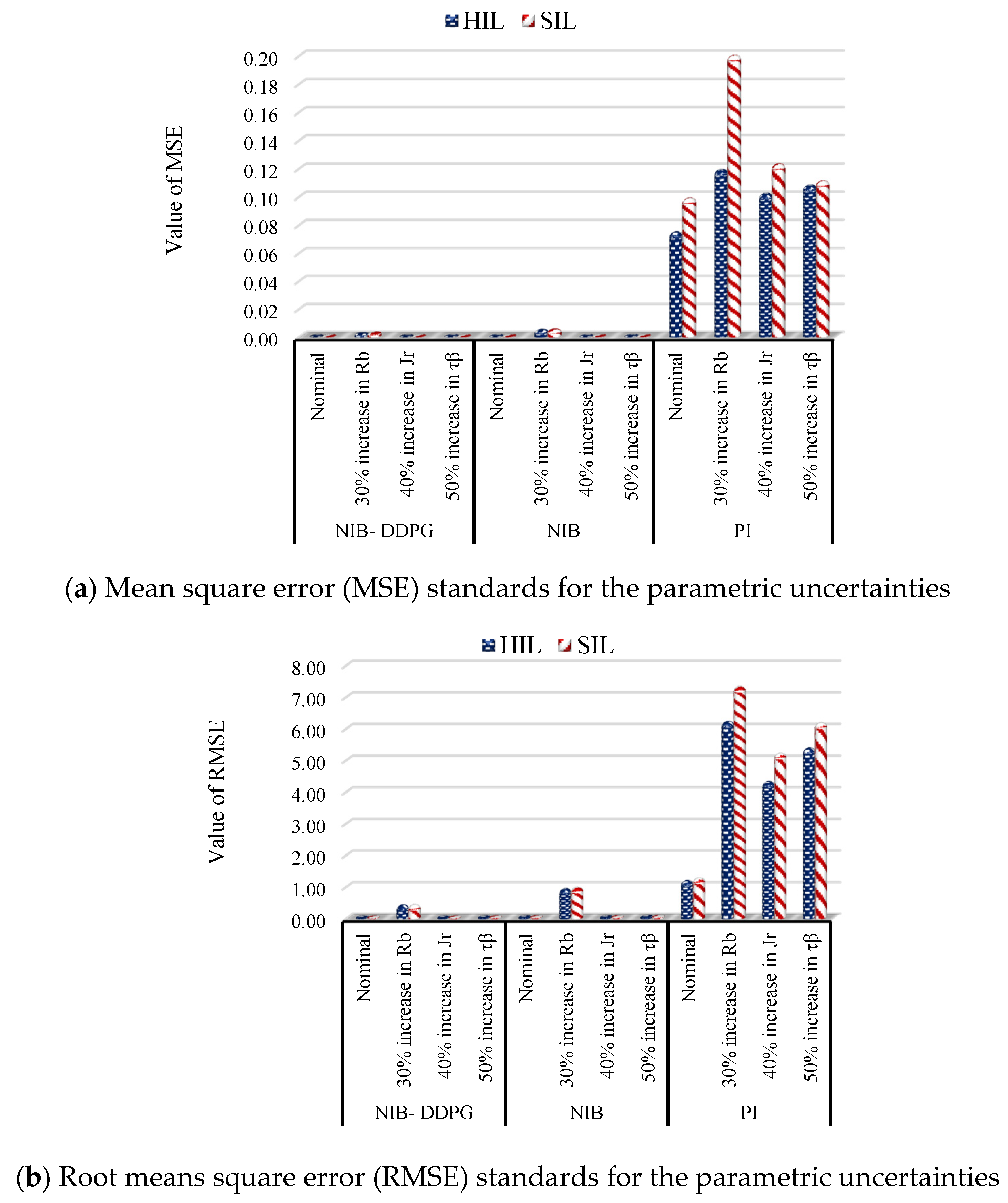
5.3. Scenario III (The Parametric Uncertainty in the Turbine Model)
6. Conclusions
Author Contributions
Funding
Conflicts of Interest
References
- Rezaei, V. Advanced control of wind turbines: Brief survey, categorization, and challenges. In Proceedings of the 2015 American Control Conference (ACC), IEEE, Chicago, IL, USA, 1–3 July 2015; pp. 3044–3051. [Google Scholar]
- Chen, J.; Chen, J.; Gong, C. New Overall Power Control Strategy for Variable-Speed Fixed-Pitch Wind Turbines within the Whole Wind Velocity Range. IEEE Trans. Ind. Electron. 2012, 60, 2652–2660. [Google Scholar] [CrossRef]
- Boukhezzar, B.; Siguerdidjane, H. Nonlinear Control of a Variable-Speed Wind Turbine Using a Two-Mass Model. IEEE Trans. Energy Convers. 2010, 26, 149–162. [Google Scholar] [CrossRef]
- Leithead, W.E.; De La Salle, S.A.; Reardon, D. Classical control of active pitch regulation of constant speed horizontal axis wind turbines. Int. J. Control. 1992, 55, 845–876. [Google Scholar] [CrossRef]
- Wright, A.D. Modern Control Design for Flexible Wind Turbines; National Renewable Energy Laboratory: Golden, CO, USA, 2004. [Google Scholar]
- Lather, J.; Dhillon, S.; Marwaha, S. Modern control aspects in doubly fed induction generator based power systems: A review. Int. J. Adv. Res. Electr. Electr. Instrum. Eng. 2013, 2, 2149–2161. [Google Scholar]
- Trabelsi, R.; Khedher, A.; Mimouni, M.F.; M’Sahli, F. An Adaptive Backstepping Observer for on-line rotor resistance adaptation. Int. J. IJ-STA 2010, 4, 1246–1267. [Google Scholar]
- Ullah, N.; Wang, S. High performance direct torque control of electrical aerodynamics load simulator using adaptive fuzzy backstepping control. Proc. Inst. Mech. Eng. Part G J. Aerosp. Eng. 2014, 229, 369–383. [Google Scholar] [CrossRef]
- Rajendran, S.; Jena, D. Backstepping sliding mode control of a variable speed wind turbine for power optimization. J. Mod. Power Syst. Clean Energy 2015, 3, 402–410. [Google Scholar] [CrossRef] [Green Version]
- Fliess, M.; Join, C. Model-free control and intelligent pid controllers: Towards a possible trivialization of nonlinear control? IFAC Proc. Vol. 2009, 42, 1531–1550. [Google Scholar] [CrossRef] [Green Version]
- Fuglsang, P.; Madsen, H.A. Optimization method for wind turbine rotors. J. Wind. Eng. Ind. Aerodyn. 1999, 80, 191–206. [Google Scholar] [CrossRef]
- Selig, M.S.; Coverstone-Carroll, V.L. Application of a Genetic Algorithm to Wind Turbine Design. J. Energy Resour. Technol. 1996, 118, 22–28. [Google Scholar] [CrossRef] [Green Version]
- Wiering, M.; Van Hasselt, H. Ensemble Algorithms in Reinforcement Learning. IEEE Trans. Syst. Man Cybern. Part B (Cybern.) 2008, 38, 930–936. [Google Scholar] [CrossRef] [Green Version]
- Watkins, C.J.C.H. Learning from Delayed Rewards; King’s College: London, UK, 1989. [Google Scholar]
- Rummery, G.A.; Niranjan, M. On-Line Q-Learning Using Connectionist Systems; University of Cambridge, Department of Engineering Cambridge: Cambridge, UK, 1994. [Google Scholar]
- Sutton, R.S. Generalization in reinforcement learning: Successful examples using sparse coarse coding. In Advances in Neural Information Processing Systems; University of Massachusetts: Amherst, MA, USA, 1996; pp. 1038–1044. [Google Scholar]
- Sutton, R.; Barto, A. Reinforcement Learning: An Introduction. IEEE Trans. Neural Netw. 1998, 9, 1054. [Google Scholar] [CrossRef]
- Wiering, M.A.; Van Hasselt, H. Two Novel On-policy Reinforcement Learning Algorithms based on TD(λ)-methods. In Proceedings of the 2007 IEEE International Symposium on Approximate Dynamic Programming and Reinforcement Learning, Honolulu, HI, USA, 1–5 April 2007; pp. 280–287. [Google Scholar] [CrossRef]
- Sutton, R.S.; McAllester, D.A.; Singh, S.P.; Mansour, Y. Policy gradient methods for reinforcement learning with function approximation. In Advances in Neural Information Processing Systems; AT&T Labs-Research: Florham Park, NJ, USA, 2000; pp. 1057–1063. [Google Scholar]
- Baxter, J.; Bartlett, P. Infinite-Horizon Policy-Gradient Estimation. J. Artif. Intell. Res. 2001, 15, 319–350. [Google Scholar] [CrossRef]
- Moore, A.W.; Atkeson, C.G. Prioritized sweeping: Reinforcement learning with less data and less time. Mach. Learn. 1993, 13, 103–130. [Google Scholar] [CrossRef] [Green Version]
- Riedmiller, M. Neural Fitted Q Iteration—First Experiences with a Data Efficient Neural Reinforcement Learning Method. In European Conference on Machine Learning; Springer: Berlin/Heidelberg, Germany, 2005; Volume 3720, pp. 317–328. [Google Scholar]
- Pang, H.; Gao, W. Deep Deterministic Policy Gradient for Traffic Signal Control of Single Intersection. In Proceedings of the 2019 Chinese Control and Decision Conference (CCDC), Nanchang, China, 3–5 June 2019; pp. 5861–5866. [Google Scholar]
- Ghouri, U.H.; Zafar, M.U.; Bari, S.; Khan, H.; Khan, M. Attitude Control of Quad-copter using Deterministic Policy Gradient Algorithms (DPGA). In Proceedings of the 2019 2nd International Conference on Communication, Computing and Digital systems (C-CODE), Islamabad, Pakistan, 6–7 March 2019; pp. 149–153. [Google Scholar]
- Glaessgen, E.; Stargel, D. The Digital Twin Paradigm for Future NASA and U.S. Air Force Vehicles. In Proceedings of the 53rd AIAA/ASME/ASCE/AHS/ASC Structures, Structural Dynamics and Materials, Honolulu, HI, USA, 23–26 April 2012; p. 1818. [Google Scholar]
- Tao, F.; Sui, F.; Liu, A.; Qi, Q.; Zhang, M.; Song, B.; Guo, Z.; Lu, S.C.-Y.; Nee, A.Y.C. Digital twin-driven product design framework. Int. J. Prod. Res. 2018, 57, 3935–3953. [Google Scholar] [CrossRef] [Green Version]
- Rajendran, S.; Jena, D. Control of Variable Speed Variable Pitch Wind Turbine at Above and Below Rated Wind Speed. J. Wind. Energy 2014, 2014, 1–14. [Google Scholar] [CrossRef] [Green Version]
- Boukhezzar, B.; Siguerdidjane, H. Comparison between linear and nonlinear control strategies for variable speed wind turbines. Control Eng. Pr. 2010, 18, 1357–1368. [Google Scholar] [CrossRef]
- Ren, Y.; Li, L.; Brindley, J.; Shangguan, X.-C. Nonlinear PI control for variable pitch wind turbine. Control. Eng. Pr. 2016, 50, 84–94. [Google Scholar] [CrossRef] [Green Version]
- Al Younes, Y.; Drak, A.; Noura, H.; Rabhi, A.; El Hajjaji, A. Robust Model-Free Control Applied to a Quadrotor UAV. J. Intell. Robot. Syst. 2016, 84, 37–52. [Google Scholar] [CrossRef]
- Al Younes, Y.; Drak, A.; Noura, H.; Rabhi, A.; El Hajjaji, A. Nonlinear Integral Backstepping─Model-Free Control Applied to a Quadrotor System. In Proceedings of the 10th International Conference on Intelligent Unmanned Systems, Montreal, Canada, 29 September–1 October 2014. [Google Scholar]
- Wei, C.; Zhang, Z.; Qiao, W.; Qu, L. Reinforcement-Learning-Based Intelligent Maximum Power Point Tracking Control for Wind Energy Conversion Systems. IEEE Trans. Ind. Electron. 2015, 62, 6360–6370. [Google Scholar] [CrossRef]
- Gu, S.; Lillicrap, T.; Sutskever, I.; Levine, S. Continuous Deep Q-Learning with Model-based Acceleration. In Proceedings of the International Conference on Machine Learning, New York, NY, USA, 12–18 July 2016; pp. 2829–2838. [Google Scholar]
- Srinivasan, S.; Lanctot, M.; Zambaldi, V.; Perolat, J.; Tuyls, K.; Munos, R.; Bowling, M. Actor-Critic Policy Optimization in Partially Observable Multiagent Environments. In Advances in Neural Information Processing Systems; Advances in Neural Information Processing Systems: New York, NY, USA, 2018; pp. 3422–3435. [Google Scholar]
- Hasanvand, S.; Rafiei, M.; Gheisarnejad, M.; Khooban, M.-H. Reliable Power Scheduling of an Emission-Free Ship: Multi-Objective Deep Reinforcement Learning. IEEE Trans. Transp. Electrif. 2020, 1. [Google Scholar] [CrossRef]
- Gheisarnejad, M.; Khooban, M.H. An Intelligent Non-integer PID Controller-based Deep Reinforcement Learning: Implementation and Experimental Results. IEEE Trans. Ind. Electron. 2020, 1. [Google Scholar] [CrossRef]
- Hajihosseini, M.; Andalibi, M.; Gheisarnejad, M.; Farsizadeh, H.; Khooban, M.-H. DC/DC Power Converter Control-Based Deep Machine Learning Techniques: Real-Time Implementation. IEEE Trans. Power Electron. 2020, 1. [Google Scholar] [CrossRef]
- Khooban, M.H.; Gheisarnejad, M. A Novel Deep Reinforcement Learning Controller Based Type-II Fuzzy System: Frequency Regulation in Microgrids. IEEE Trans. Emerg. Top. Comput. Intell. 2020, 1–11. [Google Scholar] [CrossRef]
- Rodriguez-Ramos, A.; Sampedro, C.; Bavle, H.; De La Puente, P.; Campoy, P. A Deep Reinforcement Learning Strategy for UAV Autonomous Landing on a Moving Platform. J. Intell. Robot. Syst. 2018, 93, 351–366. [Google Scholar] [CrossRef]
- Gheisarnejad, M.; Farsizadeh, H.; Tavana, M.-R.; Khooban, M.H. A Novel Deep Learning Controller for DC/DC Buck-Boost Converters in Wireless Power Transfer Feeding CPLs. IEEE Trans. Ind. Electron. 2020, 1. [Google Scholar] [CrossRef]
- Zeitouni, M.J.; Parvaresh, A.; Abrazeh, S.; Mohseni, S.-R.; Gheisarnejad, M.; Khooban, M.-H. Digital Twins-Assisted Design of Next-Generation Advanced Controllers for Power Systems and Electronics: Wind Turbine as a Case Study. Inventions 2020, 5, 19. [Google Scholar] [CrossRef]
- He, R.; Chen, G.; Dong, C.; Sun, S.; Shen, X. Data-driven digital twin technology for optimized control in process systems. ISA Trans. 2019, 95, 221–234. [Google Scholar] [CrossRef]


| Performance Measurements | DDPG Based NIB-MFC | PSO Based NIB-MFC | PSO Based PI | |||
|---|---|---|---|---|---|---|
| HIL | SIL | HIL | SIL | HIL | SIL | |
| Settling time | 0.02 | 0.03 | 0.06 | 0.15 | 21.6 | 23.2 |
| Overshoot | 0.196% | 0.24% | 0.28% | 0.36% | 30.7% | 35.1% |
| Error | 0.076 | 0.16 | 0.178 | 0.23 | 11.21 | 13.92 |
© 2020 by the authors. Licensee MDPI, Basel, Switzerland. This article is an open access article distributed under the terms and conditions of the Creative Commons Attribution (CC BY) license (http://creativecommons.org/licenses/by/4.0/).
Share and Cite
Parvaresh, A.; Abrazeh, S.; Mohseni, S.-R.; Zeitouni, M.J.; Gheisarnejad, M.; Khooban, M.-H. A Novel Deep Learning Backstepping Controller-Based Digital Twins Technology for Pitch Angle Control of Variable Speed Wind Turbine. Designs 2020, 4, 15. https://0-doi-org.brum.beds.ac.uk/10.3390/designs4020015
Parvaresh A, Abrazeh S, Mohseni S-R, Zeitouni MJ, Gheisarnejad M, Khooban M-H. A Novel Deep Learning Backstepping Controller-Based Digital Twins Technology for Pitch Angle Control of Variable Speed Wind Turbine. Designs. 2020; 4(2):15. https://0-doi-org.brum.beds.ac.uk/10.3390/designs4020015
Chicago/Turabian StyleParvaresh, Ahmad, Saber Abrazeh, Saeid-Reza Mohseni, Meisam Jahanshahi Zeitouni, Meysam Gheisarnejad, and Mohammad-Hassan Khooban. 2020. "A Novel Deep Learning Backstepping Controller-Based Digital Twins Technology for Pitch Angle Control of Variable Speed Wind Turbine" Designs 4, no. 2: 15. https://0-doi-org.brum.beds.ac.uk/10.3390/designs4020015