Design-Assisted of Pitching Aerofoils through Enhanced Identification of Coherent Flow Structures


1
Department of Industrial Engineering, Università degli Studi di Padova, via Venezia 1, 35131 Padova, Italy
2
Lehrstuhl für Hubschraubertechnologie, Technische Universität München, Boltzmannstr. 15, 85748 Garching, Germany
*
Author to whom correspondence should be addressed.
Designs 2021, 5(1), 11; https://0-doi-org.brum.beds.ac.uk/10.3390/designs5010011
Submission received: 30 December 2020
/
Revised: 21 January 2021
/
Accepted: 8 February 2021
/
Published: 14 February 2021
(This article belongs to the Section Vehicle Engineering Design)
Abstract
:This study discusses a general framework to identify the unsteady features of a flow past an oscillating aerofoil in deep dynamic stall conditions. In particular, the work aims at demonstrating the advantages for the design process of the Spectral Proper Orthogonal Decomposition in accurately producing reliable reduced models of CFD systems and comparing this technique with standard snapshot-based models. Reynolds-Averaged Navier-Stokes system of equations, coupled with SST turbulence model, is used to produce the dataset, the latter consisting of a two-dimensional NACA 0012 aerofoil in the pitching motion. Modal analysis is performed on both velocity and pressure fields showing that, for vectored values, a proper tuning of the filtering process allows for better results compared to snapshot formulations and extract highly correlated coherent flow structures otherwise undetected. Wider filters, in particular, produce enhanced coherence without affecting the typical frequency response of the coupled modes. Conversely, the pressure field decomposition is drastically affected by the windowing properties. In conclusion, the low-order spectral reconstruction of the pressure field allows for an excellent prediction of aerodynamic loads. Moreover, the analysis shows that snapshot-based models better perform on the CFD values during the pitching cycle, while spectral-based methods better fit the loads’ fluctuations.
1. Introduction
Forward flight represents a critical operating condition for helicopters blades, and it is well known that the most crucial aspect in helicopters rotors aerodynamics concerns the composition of velocities between the advancement motion of the system and the revolution of the rotor, which results in different conditions of the incident flow. The issue involves a differential distribution of the pressure load, which increases over the advancing blade, while simultaneously decreases for its retreating counterpart. As a consequence, an imbalance of the overall moment is induced [1]. Therefore, the need to stabilise the attitude of the system entails the imposition of active control, accounting for the variation of the blades’ angle of attack. In these concerns, the most popular strategy consists in forcing the blade with a pitching motion, the latter described by a periodic law harmonised with the same period as the rotor revolution. In particular, the control system aims at increasing the angle of attack all through the advancing phase (blade azimuth angle ) and at decreasing it throughout the retreating part () [2]. However, the incidence variations can reach a certain angle of attack above the static stall condition, which may promote the aerodynamic instability of the blade; thus, a dynamic stall occurs by producing sudden excursions of the pressure load. In such conditions, forces and moments may reach values considerably higher than those loads typical of the steady case, and the possible coupling with the structure dynamics may lead to an earlier failure of the system. As a result, this event represents a propulsive limit in helicopters engineering and explains such attention paid by researchers over the years to reach a more in-depth knowledge of its occurrence [3]. Overcoming this constraint is necessary and more and more required by the increased demand for higher performance in the helicopters field, especially in the military context [4]. Although many control techniques were proposed to reduce the detrimental outcomes of dynamic stall, there is still a lack of proper awareness of the phenomenon which may drive the design process of oscillating wings, and the related subsystems [5].
Concerning the experimental side, although mentioned in previous works, the reference measurements performed for a better comprehension of the dynamic stall date back to the late 1970s and, in particular, to the pioneering works of Martin et al. [6], Carr et al. [7] and McAlister et al. [8] over a NACA 0012 aerofoil: The latter still being as milestones for the topic. Later on, a detailed physical description of the dynamic stall occurrence and attempts made to predict it was drawn by McCroskey [9]. Experiments conducted by Leishman [10] on a NACA 23012 aerofoil section showed that the evolution of a secondary vortex is typical of dynamic stall occurring at low Mach numbers. Wernert et al. [11] analysed the unsteady dynamics of an oscillating NACA 0012 aerofoil with both Particle Image Velocimetry (PIV) and laser-sheet visualisation, together with computations with Baldwin-Lomax algebraic turbulence model and stressed the strong non-reproducibility of the detached conditions during the downstroke phase. In this path, more recently, the work of Gerontakos [12] has become the most popular experimental reference for the academic community involved in computational modelling.
On the other hand, numerical modelling still struggles the inherent complexity related to the dynamics stall phenomenon, which is dominated by unsteadiness and flow characters ranging from laminar to turbulent. As a consequence, satisfactory numerical investigations became possible only with the gradual evolution of computing resources and computational techniques applied to Computational Fluid Dynamics (CFD). Even if Large-Eddy Simulations (LES) are increasingly feasible in the field of aerodynamics problems, also accounting for moving objects [13,14,15], at present the solution of Unsteady Reynolds-Averaged Navier-Stokes (URANS) equations, together with a turbulence closure model, consists of the most widely spread approach. Standard closure techniques for the URANS environment involve adopting one or two additional equations, from which the corresponding names are referred to as 1- or 2-equation models. As regards the first class, the literature shows promising results by the adoption of the Spalart-Allmaras model [16], for both compressible [17,18] and incompressible cases [19,20]. A variant of the model was proposed by Edwards and Chandra [21] the so-called Spalart Allmaras with Edwards modification (SAE). The different formulation of the turbulence production term has proved that a proper tuning of the model may improve the prediction abilities of the standard approach [22,23], even in the field of retreating blade stall [24]. A detailed 2D-based comparison study concerning the role of the seven different turbulence models can be found in Singh and Páscoa [25] while similar analysis are provided by Wang et al. [26]. The latter authors discussed the difference between standard and SST for a low-Reynolds two-dimensional case experiencing dynamic stall evolution. The work was expanded by Wang et al. [27] who accounted for the third dimension and compared standard URANS computations with a Detached Eddy Simulation (DES) approach: in particular, the former was coupled with either RNG and Transition SST (also known as Re), while the latter was solved together with SST. In Kai et al. [28] available experimental data are reproduced through a 2D model. Simulations are conducted with overset mesh technique, by solving URANS equations together with SST closure model. A further simulation is performed with the addition of coupled plunging and pitching conditions to assess the effects on the dynamic stall of the phase difference between the two motions. In recent times, Marchetto and Benini [29] numerically addressed the pitching motion on a 2D RAE 2822 aerofoil. Attention was paid to the impact of height and chordwise location of Gurney flaps on the loads during flow evolution.
In some way, recognising the organisation underlying a phenomenon is the first step toward a better comprehension of the phenomenon itself. This lies in an enhanced ability to reproduce it even through simplified models which are, however, able to describe its features as reliably as with the demanding CFD approach. It is in this spirit that, starting from the 1970s, the identification of coherent structures in turbulent flows has become a central issue for the research community [30]. To this end, a significant contribution was given by Lumley [31] with the introduction of Proper Orthogonal Decomposition (POD) in the context of fluid mechanics. The method extracts the coherent structures through a modal decomposition, without the need to account for conditional criteria. The minimisation of the projection error guarantees the energetic optimality in the sense of the norm [32]. Thus, from either numerical or experimental data, the optimal projection basis is obtained by solving a classical eigenvalue problem. The energy modal ranking allows for a selection of highly correlated modes which are isolated from the high-order contributions, usually characterised by a significant signal-to-noise-ratio [33]. However, since the turbulence complexity is still an open issue, the identification of organised characters represents the first step toward a more-in-depth comprehension of its nature and possible ways to control turbulent phenomena [34]. To this purpose, the great appeal of POD lies in its being a linear procedure that, nevertheless, puts no linearity conditions on the problem where it is applied to [35,36]. Different formulations of the theory were devised over the years to enhance its suitability for turbulent issues and, currently, the most popular POD-based technique is the so-called snapshot-POD by Sirovich [37]. More recently, Sieber et al. [38] proposed a spectral variation of the procedure; thus, named Spectral Proper Orthogonal Decomposition (SPOD). The method is grounded on the application of finite impulse response filter along with the diagonals of the POD correlation matrix. In particular, the methodology aims to redistribute the energy among the modes; thus, increasing the signal-to-noise-ratio of the higher-order structures. As a result, it is possible to recover new coherent structures that were previously hidden as the noise of the low-order modes, resulting in a chance to extract novel dynamics and flow properties that were once unknown. The method was already successfully adopted by Sieber et al. [39] in the modal analysis of a swirl-stabilised combustor flow resulting from measurements with Particle Image Velocimetry (PIV). In particular, the study showed the SPOD’s ability to extract the coherent structures related to the swirl flames accurately. Similarly, Lückoff et al. [40] addressed the impact of seven different actuators on the flow of a swirl-stabilised combustor showing the SPOD capability to draw the differences between the flow dynamics connected with two of the geometries. In Ribeiro and Wolf [33], the modal analysis is conducted on a flow past a NACA 0012 aerofoil at a fixed incidence angle, solved with the LES approach. The investigation focused on an extensive comparison between snapshot POD, spectral POD and Fourier-POD regarding the extraction of organised flow features connected with the noise generated on the computational domain. Ricciardi et al. [41] compared POD and SPOD concerning the identification of coherent structures inside the cavity of landing gear and accounting for a 3D-model DES database. The study proved that spectral POD variation showed superior ability in recovering enhanced harmonic correlations of the structures connected with the tonal noise in the cavity. Finally, a first attempt at studying dynamic stall through SPOD can be found in Wen and Gross [1]. Here, Implicit Large-Eddy Simulations were carried out over a Sikorsky SCC-A09 aerofoil undergoing three different configurations of motion, respectively: pitching & surging, pitching & surging & rotation, and pitching & surging & yawing.
The copious production related to dynamic stall agrees upon the fact that the phenomenon is not yet entirely ascertained. This supports the intention to address the problem through novel approaches that were not previously considered. The definition of a new procedure that provides novel insights into the issue is expected by the research community, in that this would represent a solid backbone for the design of lifting rotors. In this regard the SPOD results in a promising strategy. The present work aims at introducing this enhanced tool as one of crucial importance in the investigation of dynamic stall, providing new insights into the flow dynamics and extracting previously hidden structures that may lead to a better knowledge of its nature. In this path, this novel technique emerges from the previous approaches as a further step towards an improved and reliable magnification on the innermost organisation of the turbulence dynamics. According to the expertise gained by the authors, this investigation represents the first attempt to provide a detailed framework for a proper tuning of the spectral decomposition in the context of oscillating aerofoils. The SPOD is applied to the numerical database obtained from simulations of a two-dimensional NACA 0012 aerofoil undergoing pitching motion, by decomposing the velocity and the pressure fields. The flow configuration is that of a case study of interest for the research group, in that it is currently part of an enhanced design preliminary study. Thus, the main intention is to assess the effects of the filter on the dynamics of a flow in deep dynamic stall conditions when this is applied to both vector- and scalar-valued fields. The analysis is performed by inspection of time and spatial behaviour of the modes and by reconstruction of the database with a low-order approach.
The paper is organised as follows: In Section 2, the main properties of the POD and SPOD are outlined. Section 3 focuses on the geometrical model and the computational domain. The solver is introduced as well, and simulations setups are drawn. Section 4 presents the results. Numerical solutions from simulations are first discussed, then the modal analysis is thoroughly addressed. Finally, Section 5 provides the conclusive remarks and the future developments.
2. Spectral Proper Orthogonal Decomposition
Turbulent flows are characterised by a broad spectrum of time and spatial scales whose evolution has always drawn the attention of the research community [34]. Although addressed as an organised phenomenon already from the late 1950s, the first mention of coherent structures underlying turbulence should be referred to the work from Brown and Roshko in 1971 [30]. At that time, Lumley [31] had already introduced the Proper Orthogonal Decomposition (POD) as an unbiased tool to extract organised characters from turbulent flows, which became, henceforth, widespread.
In the present work, the spectral variation of the POD proposed by Sieber et al. [38] is employed. A detailed mathematical assessment of the method can be found in Sieber et al. [42] while here the authors follow a brief description. The technique stems from the snapshot POD [37], where a signal is divided into its ensemble average and a fluctuating component . Thus, the signal is expanded as a spatial modes series
where denotes the modal components and the time coefficients. Here denotes the number of snapshots, i.e., the collection of time instants for which the flow variable is defined.
The determination of the optimal projection basis is then addressed as a classical constrained optimisation problem. From the calculus of variations theory, it is possible to prove that the problem can be reformulated in terms of an eigenvalue problem for the correlation matrix. In particular, the correlation between two snapshots should be intended in the sense of the inner product, , as:
where D denotes the variable domain of definition. As a result, in a discrete path the snapshot correlation yields to the correlation matrix as:
Here is the snapshots matrix, i.e., the matrix which collects all the fluctuations as columns while is a diagonal matrix containing the cells volume weighting, transferred at all the nodes. Such theoretical arrangement accounts for the computations of the time-coefficients which are subjected to the following eigenvalues problem
thus, being the eigenvectors of the matrix. Here the eigenvalues, , are also known as modal energies, representing the fraction of the initial signal which belong to the corresponding reconstructed mode. Spatial modes (or coherent structures) are recovered from projection of the original signal onto the basis of time coefficients as
The results obtained from the decomposition may then be adopted for the definition of a reduced-order model, as suggested by Equation 1. Thus, the energetic ranking based on the eigenvalues provides a natural criterion to select the modes containing the most correlated and energetic characters of the signal. Accordingly, the normalised cumulative sum of the energy, , is used as a leading parameter in getting a quantitative datum concerning the number of modes which should be retained for the signal reconstruction; the latter holds as:
The procedure described so far for the snapshot POD is revisited by Sieber et al. [38] in a spectral variation and, in this sense, is called Spectral Proper Orthogonal Decomposition (SPOD). This novel technique is based on the application of a low-pass filter, along with the diagonals of the correlation matrix. The filter, g, is of size . The problem is then re-assessed for the modified correlation matrix, , the latter defined as:
Thus, an eigenvalues problem is solved as in POD and, for the sake of clarity, the nomenclature is re-defined for the energies , the time coefficients , and spatial modes . The role of the filter consists of increasing the modal signal-to-noise-ratio by redistributing the energy among the modes ensuring the preservation of whole dynamic content. As a result, for the first modes, the values of are lower than the corresponding values of . Furthermore, the method provides a tool to continuously shift from the snapshot POD () to the Discrete Fourier Transform (DFT) (). Sieber et al. [38] also propose a method to couple modes connected with periodic structures, which can be interpreted as a single complex quantity, , defined as:
The technique adopts the Dynamic Mode Decomposition (DMD) of the time coefficients to identify and rank the pairs according to the harmonic correlation. In addition, the pair energy and corresponding weighted averaged frequency are computed. Both the techniques stem from the correlation matrix’s computation, as the weighted inner product of the snapshot matrix. Although the weighting matrix, , is diagonal, the dense nature of makes it impossible to take advantage of the convenient compact storage framework for the computation of Equation (3). This may raise scepticism about the applicability of the analysis in three-dimensional problems, where the rows of the snapshot matrix may reach dimensions that are prohibitive for common computational resources. Anyhow, it is essential to recall that in general one is interested in recovering the most energetic structures. This allows for decreasing the dimension of the problem either by selecting a proper smaller region of interest [41] or by taking advantage of peculiar symmetries. The latter reducing the problem to an actual 2D decomposition of the spanwise averaged quantities [1]. When the nature of the investigation is such that a massive grid region must be considered, a solution could be to implement a code through the Message Passing Interface (MPI) [33].
3. Computational Setup
The numerical analysis reproduces the experimental setup of Lee and Gerontakos [43]. Thus, a NACA 0012 aerofoil is chosen with a chord length m as sketched in Figure 1. The measurements were carried out on a finite wing with a span equal to 2.5 times the chord and adopting endplates to reduce the tip effects. In particular, hotwire probes showed a two-dimensional non-uniformity of the flow over the wing bounded to . Based on this evidence, in agreement with the assumption of Wang et al. [26], the present work considers it reasonable to adopt a 2D model.
The computational domain is built as a double-block O-Grid with an overlapping region and the mesh is created as three-dimensional with a single cell along the span. The inner block is generated with quadrilateral elements around the aerofoil and extends up to 1.7 times the chord, starting from the quarter chord location. This point coincides with the centre of the whole mesh and defines the pole of the pitching motion. As usual in pitching analysis, the rotating motion develops about the y-axis. A first layer of cells is wall-normally extruded, starting from a nominal initial distance of . Here is the fluid density at the wall location, is the friction velocity, is the distance of the first grid point and is the fluid laminar wall viscosity. The friction speed is estimated based on aerofoil chord and the maximum of the considered free stream velocities (see Table 1). This choice is conservative for the experimental setup configuration which involves less critical boundary conditions. Nodes distribution is thickened in the neighbourhood of leading and trailing edges. Then the distribution of the elements’ sizes toward the edge of the block followed a root mean square principle.
The outer block is mainly composed of triangular elements, except for a refined structured region behind the aerofoil that extends up to 6 times the chord of the aerofoil. The far-field boundary is located at a distance of , and the mesh counts about elements with a maximum equiangular skewness lower than 0.69. An equiangular skewness value lower then 0.37 is reserved in the structured region Figure 2 reports the overall mesh (Figure 2a) an the magnification of the leading and trailing edges of the aerofoil (Figure 2b,c).
The set of the simulations aim at tracing the unsteady behaviour of the flow during pitching, focusing in particular, on deep dynamic stall conditions. In particular, the aerofoil pitch angle is varied through a monochromatic sinusoidal law which holds as:
Here is the time-depending pitch angle, its offset and denote its amplitude. k is the reduced frequency of the system and its angular frequency. The reference Reynolds number is based on the flow free stream density and viscosity and the free stream speed . The simulation data initially follow the experimental assessment of Lee and Gerontakos [43]. Then a case study setup is adopted to run simulations from which data are extracted for the spectral analysis. As stated in the introduction, such workflow falls in the context of a preliminary investigation aiming to improve the definition of the design parameters for an applicative configuration. For this reason, the numerical assessment has been primarily tested on the well-documented low-Mach conditions [43]. However, being the latter very far from real applications, a test case configuration is further analysed. A complete summary of the simulated conditions is listed in Table 1.
Concerning the boundaries, the latter are prescribed as follow: A far-field condition is chosen for the outflow edges, while symmetry is enforced at the ends of the aerofoil span. To solve the flow between the overlapping zones, the free edges of the two blocks corresponding to the overset region are set as Chimera boundary condition. The Chimera boundaries technique is efficiently implemented in TAU [44,45,46,47] and in this case allowed for building a customised refinement without the need to impose motion on the whole grid. According to this technique, also known as simply overset grid, multiple blocks are built with overlapping common zones. A hole is cut on blocks where non-penetrable surfaces are identified, then the information is transferred between different blocks by interpolating over the overlapping cells at the boundary of the hole [48]. It is essential to consider that such grid structure favours a higher resolution in the wake region and provides greater accuracy in heading the detached flow dynamics, which was not achievable with a simple O-grid. In particular, the latter would have required a much denser grid overall and, consequently, higher demand for computational resources. Instead, splitting the domain into blocks allowed for adopting an unstructured grid for a more significant part of the far-field domain.
The computations are performed using the TAU-solver by DLR. The solver has been extensively validated by previous publications [44,49,50,51] both performing 2D and 3D Navier-Stokes analysis. In the present work, the Unsteady Reynolds-Averaged Navier-Stokes (URANS) system of equations is solved using explicit dual time stepping. The convective fluxes are discretised through a central difference scheme with scalar dissipation, while turbulent scalars employ an upwind scheme. Time-integration takes advantage of a backward Euler relaxation method combined with Lower-Upper Symmetric Gauss-Seidel (LU-SGS) linear solver.
Concerning the turbulence model, both the 1-equation Spalart-Allmaras model with Edwards modification (SAE) and the 2-equation Shear Stress Transport (SST) model by Menter (2003) are used. Unsteady simulations are initialised from a steady-state condition; the latter solved up to 3000 iterations. Four complete pitching periods are computed, thus showing flow stabilisation starting from the third. Pitching cycles are discretised with 3600 time-steps, each solved for a maximum of 300 inner iterations. Stop criterion for iterations is set at a condition where root mean square of the residuals is equal to , and monitoring the relative fluctuation on the density, re-normalised at the beginning of each time step. This strategy for monitoring the residuals is chosen to promote the convergence of the single time step, especially for the ones related to the most critical flow conditions at the highest incidences. In this regard, the maximum number of inner iterations guarantees convergence for those steps, though being oversized for the remainder. The choice of the time discretisation is consistent with sampling at least 100 flow events over a single pitching cycle. The chosen physical time size evolves almost 155 times in the convective time scale of the flow, based on the most critical boundary conditions, i.e., .
Figure 3 shows the non-dimensional vorticity field distribution corresponding the instant where . The configuration preludes the Leading Edge Vortex (LEV) sheds into the wake; thus it slightly advances the dynamic stall condition.
4. Results and Discussion
4.1. Simulation Results Compared to Experimental Setup
In order to assess the ability of the numerical model in accurately heading the flow dynamics connected with the pitching motion of the aerofoil, a primary set of numerical simulation is carried out and compared to the experimental data by Lee and Gerontakos [43] in corresponding flow conditions. In particular, Figure 4 shows the numerical aerodynamic coefficients (round dots) as a function of the angle of attack and compared to experimental measurements (black dots). From the obtained results, the current model is unable to head the system’s dynamics quite accurately, even during the dynamic stall evolution. In particular, the linear phase of the load is in excellent agreement with the experimental data for both the SAE and the SST turbulence models. The curves diverge as the boundary layer thickens without detachment even above the stall condition in steady-state (i.e., around 15°). In particular, the numerical assessment anticipates the shedding of the primary vortex into the wake; the latter being the cause of the lift stall. The model predicts this event at 22.3° and 22.6° for SAE and SST, respectively, instead of 24.3° for experimental arrangement. At this stage, forces prediction are underestimated for the lift, while overestimated for the drag.
However, the most significant discrepancy between numerics and measurements can be identified in the presence of a second vortex, which was undetected by Lee and Gerontakos [43]. This additional flow feature is probably the result of the present 2D approximation that struggles the inherent three-dimensional character dominating the flow evolution, especially at high angles of attack. In this circumstance, the pitch moment reaches the (negative) peak value for both the turbulence models. As regards the SAE, this event coincides with a second peak of the drag force that is stronger than the first, while when considering the SST closure, this second peak is still lower than that connected with the primary vortex. The inspection of the flow field distribution showed that this vortex rapidly forms at the trailing edge.
Concerning the downstroke phase, the two turbulence models predict a markedly different flow evolution. In particular, the SAE estimates the formation of a different structure that causes a second peak of the lift force, which is even more significant than the value connected with the lift stall. The same effect can be seen in the drag plot, while in the moment coefficient, this event generates a second significant load condition. However, a similar fluctuation can also be detected in the SST plot. In any case, both the turbulence closures depart from the experimental flow evolution. Measurements, in fact, show to nearly recover the linear trend, though with lower values, while the numerical model is affected by the flow structures developing during the phase of fully detached flow. In particular, when considering the SAE model, it is possible to see an intense excursion of the loads between 20° and 10° that leads the flow to reach greater load values than the ones predicted by the static theory. This is incompatible with the known character of the flow during this phase and may be considered as clear evidence of the inability of the present model to reconstruct the phenomenon of dynamic stall. The concluding part of the downstroke is characterised by a general approach between the numerical results and experiments, especially in what concerns drag and moment loads. In fact, from the lift coefficient, it is possible to see how measurements suggest that the flow recovers the static theory behaviour only after the null angle of attack. At the same time, the hysteresis detectable in the negative incidence phase highlights that the flow is still subject to unsteady and possibly 3D characters. This behaviour is not recovered by numerics, where the hysteresis is missing, and the flow evolution follows the linear theory. The present results from the 2-equation model are found in good agreement with other published numerical assessments based on the same experimental data-set [25,26].
4.2. Simulation with Case Study Conditions
After analysing the response of the numerical model against the experimental data of Lee and Gerontakos [43], the 2-equations SST turbulence model is selected to simulate the case study conditions for the design (see Table 1 for the details). The grid’s quality regarding this simulation was determined based on the evolution of the throughout the pitching cycle. As reported in Figure 5, the maximum value reached at the end of each time step is limited to 1.8, even for the most critical conditions experienced by the flow. Such value falls in every RANS simulation’s best-practice and is consistent with the selected turbulence model, which generally requires a maximum of on the walls around the unity. For this reason the present mesh has been considered capable of accurately heading the system’s dynamics. It is necessary to clarify that this simulation setup involved shocked-induced effects as the boundary layer’s driving factors thickened at the leading edge; then promoting the dynamic stall [52]. However, these events do not result in coherent structures in the decomposition process (discussed later on) giving minor importance to the declared purpose of the present work: i.e., to present a possible novel framework to be applied in the context of numerical data-set concerning oscillating aerofoils.
In particular, the obtained results in this secondary arrangement show a smoother behaviour of the loads’ curves (Figure 6), which reflects the presence of a lower number of turbulent structures developing throughout. According to the coefficients’ trends, the flow’s evolution presents some similarities with previous results. In particular, the linear behaviour ![Designs 05 00011 i001]() follows the same trace until the steady-state angle of attack is reached (Figure 6a). Here, again, the slope of the curve briefly flattens
follows the same trace until the steady-state angle of attack is reached (Figure 6a). Here, again, the slope of the curve briefly flattens ![Designs 05 00011 i002]() before becoming even greater than in the linear trend. This condition also induces a drop of the moment curve (Figure 6c). The reason for this can be ascribed to the gradual thickening of the boundary layer that generates the leading edge vortex, whose low-pressure core travels down to the trailing edge throughout the motion. As it passes the centre of pressure of the aerofoil, the negative effect of the moment drastically increases. This process continues in full attachment conditions, which explains the protracted trend of the loads. After lift stall occurs, with the vortex shedding at
before becoming even greater than in the linear trend. This condition also induces a drop of the moment curve (Figure 6c). The reason for this can be ascribed to the gradual thickening of the boundary layer that generates the leading edge vortex, whose low-pressure core travels down to the trailing edge throughout the motion. As it passes the centre of pressure of the aerofoil, the negative effect of the moment drastically increases. This process continues in full attachment conditions, which explains the protracted trend of the loads. After lift stall occurs, with the vortex shedding at ![Designs 05 00011 i003]() , the load along the z axis shows an almost monotonic behaviour. Differently, the sudden formation of a trailing edge vortex affects both the drag (Figure 6b) and moment loads. The appearance of a trailing edge vortex is depicted by a second peak in the two plots
, the load along the z axis shows an almost monotonic behaviour. Differently, the sudden formation of a trailing edge vortex affects both the drag (Figure 6b) and moment loads. The appearance of a trailing edge vortex is depicted by a second peak in the two plots ![Designs 05 00011 i004]() and in particular, for the moment load, this value represents the maximum negative excursion. The concluding part of the upstroke phase is influenced by a brief re-attachment of the circulating flow. In fact, in the neighbourhood of the maximum incidence, the three aerodynamics coefficients show a rapid, though limited, excursion
and in particular, for the moment load, this value represents the maximum negative excursion. The concluding part of the upstroke phase is influenced by a brief re-attachment of the circulating flow. In fact, in the neighbourhood of the maximum incidence, the three aerodynamics coefficients show a rapid, though limited, excursion ![Designs 05 00011 i005]() . As can be seen from the flow distribution, this event is generated by a circulation bubble that extends over the whole aerofoil and has a low-pressure core located beyond the centre of pressure. The remainder of the flow evolution
. As can be seen from the flow distribution, this event is generated by a circulation bubble that extends over the whole aerofoil and has a low-pressure core located beyond the centre of pressure. The remainder of the flow evolution ![Designs 05 00011 i006]() develops with conditions typical of full detachment. Here, the small fluctuations seem to be mostly related to the numerics and not to the physics of the system.
develops with conditions typical of full detachment. Here, the small fluctuations seem to be mostly related to the numerics and not to the physics of the system.
 follows the same trace until the steady-state angle of attack is reached (Figure 6a). Here, again, the slope of the curve briefly flattens
  before becoming even greater than in the linear trend. This condition also induces a drop of the moment curve (Figure 6c). The reason for this can be ascribed to the gradual thickening of the boundary layer that generates the leading edge vortex, whose low-pressure core travels down to the trailing edge throughout the motion. As it passes the centre of pressure of the aerofoil, the negative effect of the moment drastically increases. This process continues in full attachment conditions, which explains the protracted trend of the loads. After lift stall occurs, with the vortex shedding at
  , the load along the z axis shows an almost monotonic behaviour. Differently, the sudden formation of a trailing edge vortex affects both the drag (Figure 6b) and moment loads. The appearance of a trailing edge vortex is depicted by a second peak in the two plots
  and in particular, for the moment load, this value represents the maximum negative excursion. The concluding part of the upstroke phase is influenced by a brief re-attachment of the circulating flow. In fact, in the neighbourhood of the maximum incidence, the three aerodynamics coefficients show a rapid, though limited, excursion
  . As can be seen from the flow distribution, this event is generated by a circulation bubble that extends over the whole aerofoil and has a low-pressure core located beyond the centre of pressure. The remainder of the flow evolution
  develops with conditions typical of full detachment. Here, the small fluctuations seem to be mostly related to the numerics and not to the physics of the system.
4.3. Spectral Proper Orthogonal Decomposition
The above-discussed simulations are used to perform the modal analysis according to the SPOD method by Sieber et al. [38]. In particular, the flow variables are extracted for the last 2 cycles from the inner pitching block; a choice that is motivated since further investigations made by decomposing the whole computational domain showed that the dynamics of the most relevant modes remains unaltered. The sampling process is performed every 36 time-steps. After extracting the ensemble mean, the correlation matrix is computed accounting for the velocity fluctuations, considering both the and components. Then, the spatial coherence of the modes is discussed through the modes related to . According to Sieber et al. [38], three filter sizes, , are chosen. In particular, the POD analysis () is compared to the two SPOD’s levels. The former level corresponds to the time needed by the main vortex to form and shed past the observation domain; the latter, to time spent by the flow to reach full detachment conditions. The following Gaussian distribution
is used for the filtering process.
As expected, the obtained results show that the filter re-distributes the modal energies among the modes (Figure 7). In particular, Figure 7a,c,e show how the energy of the first mode is gradually reduced as the filter size increases in favour of the energy of the following modes (blue histograms). Moreover, it is possible to see that the slope of the cumulative sum curve (red dots) significantly reduces while the filter width increases. However, the dominant energy of the first modal contribution remains appreciably higher than the others: a result that reflects how the aerofoil motion strictly governs the evolution of the flow. As the curve of cumulative energies smoothens, the number of modes required to reconstruct a given percentage of the original signal increases. As a consequence, Figure 7b,d,f show that the scatter plot related to the SPOD’s spectrum gets more populated. The figures, in particular, report the percentage of the modal contributions as a function of the Strouhal number of the system; the latter defined as , where f denotes the modal frequency. In the present work, the number of modes retained for the signal reconstruction is chosen such that corresponding cumulative energy at least equal to 99% is recovered. Thus, Figure 7d highlights how the filter can extract new coherent structures corresponding to the eleventh harmonic (red spot labelled with number 3 in Figure 7d), which were not particularly correlated in the POD spectrum (Figure 7b). Moreover, it is interesting to note how a further application of the filter (Figure 7f) allows for better identification of the structure dynamics around its typical frequency.
The temporal flow dynamics stem from a deeper inspection of the coefficients of the decomposition. Here, the response of the modes in the set of frequencies is studied through the computation of Power Spectral Density (PSD) of the coupled coefficients. The PSD analysis is performed following Welch’s method [53] and it is applied to the complex entity generated by the paired modes. Contextually, phase portraits are adopted as visual evidence of the harmonic correlation between the single dynamics coupled with the procedure. Thus, Figure 8 combines the analysis of the time coefficients referred to the third pair (intended as ) to varying dimensions of the filter.
Pure POD (Figure 8a) clearly extracts a dominant frequency at the second harmonic of the motion, i.e., . However, the broadband pair’s content accounts for a broader frequency domain and, as already anticipated in Figure 7b, the correlation of the real and imaginary modal components is marginal. Accordingly, the phase diagram (Figure 8b) provides no indications on the common time evolution of the single modes. On the other hand, the time constraint introduced by the application of the filter (SPOD with ) allows for a more refined definition of the pair’s dynamic. This can be stated based on two effects depicted by the analysis of the time domain and, in particular, looking at the frequency response. In this regard, Figure 8c shows how the dominant modal contribution is now identified at the eleventh harmonic. It is important to note that this result combines two simultaneous actions: the suppression of the other responses and the enhancement of the PSD connected with the newly recognised evolution. Besides, a secondary effect is deducible from Figure 8d. Here, it is possible to read a circular shape is detectable, a structure which is typical of harmonic correlation recovered by purely spectral analysis as the Discrete Fourier Transform (DFT). The fact suggests how the two pair components are now much more correlated during the time evolution. The application of a higher filter width () is made to address the actual impact of the SPOD. To this end, the PSD of the pair (Figure 8e) highlights the filter role in further extracting the structures’ natural evolution. This aspect is depicted by the additional suppression of the broadness of the band. At the same time, the response at the eleventh harmonic is not discarded, but somewhat slightly re-enforced: a result that confirms the SPOD’s ability to inspect the innermost characters of the evolving dynamics properly. Again, the phase portrait (Figure 8f) depicts a stronger affinity with a circular outline. Both the PSD and phase diagrams show, in this case, that the filter size is shifting the decomposition toward a purely spectral analysis. However, the multi-frequency content suggests that the energetic optimality typical of POD is not entirely compromised, which draws the convenience of the present approach in dealing with the stall dynamic.
Thus, the inspection of the spatial modes is necessary to show how the action of the spectral analysis on the coherent structures is consistent with what discussed the corresponding time coefficients. As already evidenced by Taira et al. [54], travelling structures are usually described by a pair of real singles modes, whose coherent zones are shifted in the spatial domain according to the specific wavelength. In this sense, the resolution and periodicity of the coupled modes’ structures may be assumed as a measure of the related spatial coherence.
Figure 9 reports the distribution of the (single) spatial modes corresponding to the SPOD time coefficients and . Consistently with the previous analysis, the POD demonstrates a clear inability to correlate the dynamics of the two coupled modes since the spatial organisation of the structures of mode 5 (Figure 9a) depicts a generally inclined directionality that lacks the mode 6 (Figure 9b). Furthermore, the evolution provided by Figure 9a broadly distributes the wake, even over the aerofoil, denoting poor definition of the structures. Conversely, the structures showed by have a much more refined shape evolving from the middle chord to the wake. However, no periodicity can be traced with the spatial distribution of its paired mode. On the contrary, the effect of the first SPOD’s level is markedly in favour of the correlation of the two single dynamics. This is inferred based on the spatial distribution of the corresponding modes. Here, mode 5 (Figure 9c) acts as the advancing mode: as a consequence, the same pattern of the structures can be detected in mode 6 (Figure 9d), though shifted back toward the aerofoil. The fact denotes a phase delay in the spatial propagation, in line with expectations for coupled structures.
Furthermore, differently from the POD, here the directionality recovered for mode 6 allows for better identification of the correlation. Anyhow, the weaker structure over the aerofoil indicates the influence of some disturbance connected with the dynamic behaviour typical of different frequencies. Such conclusion is justified looking at Figure 9e,f where the results obtained with the SPOD’s second filter are reported. In this case, the bigger filter’s size allows for the suppression of the poorly defined regions over the aerofoil, together with a general reduction of the background noise. This holds for both the and coefficients. Moreover, one may notice that the filter has a negligible impact on the dominant flow structures and, to draw a connection with the corresponding time coefficients, this aspect is consistent with the reduced effect on the response of the eleventh harmonic already discussed and explains why the disturbances are referred to as spurious tracks connected with different frequencies. To conclude, time and spatial characters agree upon the superiority of the SPOD, when compared with POD. The enhancement provided by the former is proved by its ability to extract and adequately describe the full nature of the dynamic contents that would be otherwise hidden.
4.4. Comparison between Decompositions of Pressure and Velocity Field
As next step of the investigation the authors convey in drawing the suitability of the method when adopted for the study of a scalar field. Thus, the modal analysis is performed concerning the pressure database and following similar considerations as for the previous discussion. In particular, the filter widths for the SPOD are chosen as . Figure 10 summarises the results for the three different decompositions, concerning the energy of the paired modes as a function of the non-dimensional frequency.
As for the velocity fluctuations, the distribution of the modal dynamics on the POD spectrum is less populated (Figure 10a); the reason is always connected to the high energetic content of the first pair. This feature, in particular, recovers most of the cumulative sum of the eigenvalues, denoting how the pressure fluctuations are drastically affected by the low-order dynamics of the system motion. Although this pair of modes depicts the highest correlation among the other in the spectrum, the forthcoming inspection of the spatial structures will instead reveal a low coherence between the dynamics. One may argue that the forced coupling procedure may have the drawback of recognising paired modes even when they do not share common dynamic evolutions. The strong dependency of the modal representation on the first pair is further proved by applying the SPOD (Figure 10b). In this case, the energetic content of the first harmonic is not significantly affected, and the same holds for the average response frequency. However, the other two selected pairs demonstrate a marked sensibility of the corresponding dynamics towards the time constraint of the spectral decomposition. Although they show enhanced harmonic correlation, the mean response frequency changes drastically. In particular, the variations are from to for the second pair and from to for the third.
The application of the second filter shows a less effective action on the response of the second pair, while the third is again significantly influenced, with the mean Strouhal number shifted to (Figure 10c). Furthermore, a fourth highly correlated pair is extracted around the tenth harmonic. In general, although the filter enhances the correlation of the time coefficients, it also affects the peak response by gradually suppressing the responses at the higher frequencies. This is a different behaviour than that described for the velocity field where, instead, the action of the filter allowed for a better identification of the dominant frequency by suppressing the responses, whether they be higher or lower. This aspect reflects how the pressure field analysis is more hardly manageable, since the selection of the filter is not univocal and thus may lead to misleading interpretations of the results.
The comparison with the space modes from the velocity field shows that in general the two approaches lead to recover different structures characters. In this case, the coherent structures of the first pair obtained with the second filter are compared between the two analysis (Figure 11), since they share a comparable frequency response, i.e., around the first harmonic . In particular, and distributions are taken from SPOD, respectively with for the velocity field (Figure 11a,b) and for the pressure field (Figure 11c,d). In both the results it is possible to see the low correlation between the corresponding single modes, already suggested by the spectrum scatter plots. However it is interesting to notice that the structures described by the velocity decomposition are able to recover the dynamics associated with the second vortex, differently from what depicted by the counterparts in the pressure modes. This can be deduced by the small structure close to the quarter chord location (Figure 11b), which can be directly linked to the recirculation bubble generated by the sudden formation and attachment of the second vortex (see Figure 6). This structure is typical of the post-stall flow conditions and, differently from the LEV, is not produced by a gradual thickening of the boundary layer and contextual travel toward the trailing edge. For this reason, the structures observable in the pressure decomposition cannot be associated with the evolution of this flow feature. In fact, (Figure 11c) depicts a wide region extending over a great part of the aerofoil while the distribution of (Figure 11d) shows a clear zone connected with the dynamics around the leading edge. As a result, the evolution of the secondary vortex seems not be described by this pair as it is in the velocity decomposition.
4.5. Reconstruction of Aerodynamic Coefficients
To further investigate the differences between pure and spectral POD, the modes obtained from the pressure decomposition are employed for a low-dimensional reconstruction of the field. In particular, the analysis focuses in computing the aerodynamic coefficients from the reduced model. Figure 12 reports the re-computed values (blue line) compared to the corresponding CFD results (red line). The reduced model retains a number of modes such that the 95% of the original signal is reconstructed. As already discussed, the modal energy redistribution performed by the SPOD method accounts for a higher number of modes once the cumulative energy is chosen and, in particular, the retained modes are 7 and 12 for the POD and the SPOD, respectively. Even if the reconstructed reduced model does not account for the skin friction contribution, the results show that the general trend is well captured both by the POD and the SPOD since the system is mostly pressure-dominated. In particular, Figure 12a,c,e, report the POD results while Figure 12b,d,f, show the SPOD data corresponding to a filter width of .
Looking more in-depth insight on the results, the latter show how the SPOD better reconstructs the upstroke phase since the method is more sensitive to the loads’ fluctuations. However, it should be noted that the SPOD introduces some faulty components in terms of moment coefficient (Figure 12f), where the smoother trace depicted by the POD (Figure 12e) better approaches the CFD values. As regards the lift and the drag coefficients, the two aerodynamics coefficient are more satisfactorily reproduced by SPOD (Figure 12b,d) which is able to recover a better description of either the variations and the values of the coefficients. Especially for the lift coefficient, it is possible to see how the POD method (Figure 12a) tends to smoothen the evolution of the loads and underestimates the peak value corresponding to the dynamic stall event. On the contrary, the POD shows a superior behaviour in the drag peak’s reconstruction (Figure 12c) while the SPOD depicts a delayed angle for the occurrence of the phenomenon. Finally, both the two reconstruction methods miss the second observable peak in either the drag and moment plots: this fact may prove that the event connected with this load fluctuations relates to higher harmonics than those described by the modes here retained. To conclude, from this first analysis it is possible to state that the POD better estimates the effective values of the loads, though at delayed angles, while the SPOD better predicts the grade of the fluctuation but with a lower precision of the values. Similar words may be spent for the moment coefficient, especially for the part with negative values. The remainder of the curve shows instead a very similar behaviour.
5. Conclusions
The unsteady flow evolution of a pitching 2D NACA 0012 aerofoil is numerically investigated through Unsteady Reynolds-Averaged Navier-Stokes (URANS) equations. Computations are performed to tune either the Spalart-Allmaras turbulence model with Edwards modification (SAE) and SST model against the experimental data of Lee and Gerontakos [43]. Both the two closures show a general difficulty to reproduce the pitching phenomenon, anticipating the detachment of the Leading Edge Vortex (LEV); a result that agrees with previous references [25,26,28]. However, since the SST turbulence model shows more stable behaviour, especially regarding the downstroke phase, the model is selected for a case study simulations setup.
The CFD results are post-processed thought advanced stochastic tools and, in particular, both the Proper Orthogonal Decomposition (POD) by Sirovich [37] and the Spectral Proper Orthogonal Decomposition (SPOD) by Sieber et al. [38] are adopted. The SPOD method differs from the POD in filtering the diagonals of the correlation matrix and, in particular, the study demonstrates how a proper choice of the filter size allows for the extraction of new dynamic contents developing throughout the flow evolution. The different behaviour of the two techniques is observed concerning the post-processing of vector- and scalar-valued fields. In particular, the analysis shows how the SPOD method acts better for the velocity reconstruction while the POD better performs for pressure decomposition. The computation of the aerodynamic loads from a reduced-order reconstruction of the pressure field, compared to original CFD, benchmarks the ability of both the POD and the SPOD to recover the inherent characters of the pitching cycle.
The application of SPOD on the corresponding database shows that the filter allows for the extraction of the eleventh harmonic dynamic. In particular, for the velocity field, a wider window size enhances the response and correlation of the coherent structures around that frequency. On the contrary, the effects on the dynamics of the pressure field depict marked variations depending on the filter size. In conclusion, the aerodynamics loads’ reconstruction demonstrates that low-order models based on SPOD better perform in recovering the incidence of the oscillations occurring during the pitching cycle. However, this comes at the expense of the energetic optimality of the decomposition and, as a result, the POD-based low-order model is more reliable in reconstructing the actual values of the loads. Anyhow, forthcoming investigations are meant to dissolve the uncertainty about the behaviour of the analysis when applied to flows evolving with different Reynolds numbers. This broader study will draw a complete insight into how the results provided by this novel approach may represent an essential aid for the design process of rotorcrafts, facing a wide range of operating envelopes.
Future investigations on 3D models will also include the evolution of lower scales of turbulence. Thus, the consistency of the method will be analysed for flows where more advanced CFD techniques allow for the identification of a broader spectrum of unsteady dynamics’ characters. As a further step, the intention is to take advantage of the modes for building a reduced-order model and, thus, to prove how this can help in predicting the performance in the preliminary phase of the design process.
Author Contributions
Conceptualization, F.A. and Y.R.; methodology, F.A.; software, F.A.; validation, F.A.; formal analysis, F.A.; investigation, F.A.; data curation, F.A., F.D.V. and E.B.; writing—original draft preparation, F.A.; writing—review and editing, F.D.V., Y.R. and E.B.; supervision, F.D.V. and E.B.; project administration, E.B. All authors have read and agreed to the published version of the manuscript.
Funding
This research received no external funding.
Data Availability Statement
Data sharing not applicable.
Acknowledgments
The authors acknowledge M. Hajek from Technische Universität München (TUM) for hosting the development of the project as well as the ERASMUS+ infrastructure for making the present collaboration possible.
Conflicts of Interest
The authors declare no conflict of interest.
Abbreviations
The following abbreviations are used in this manuscript:
| CFD | Computational Fluid Dynamics |
| DES | Detached Eddy Simulation |
| DFT | Discrete Fourier Transform |
| DLR | Deutsches Zentrum für Luft- und Raumfahrt |
| DMD | Dynamic Mode Decomposition |
| ILES | Implicit Large-Eddy Simulations |
| LES | Large-Eddy Simulations |
| MPI | Message Passing Interface |
| PIV | Particle Image Velocimetry |
| POD | Proper Orthogonal Decomposition |
| PSD | Power Spectral Density |
| SAE | Spalart-Allmaras with Edwards modification |
| SPOD | Spectral Proper Orthogonal Decomposition |
| SST | Shear Stress Model |
| URANS | Unsteady Reynolds-Averaged Navier-Stokes |
References
- Wen, G.; Gross, A. Numerical Investigation of Deep Dynamic Stall for a Helicopter Blade Section. AIAA J. 2018, 57, 1434–1451. [Google Scholar] [CrossRef]
- Conlisk, A.T. Modern helicopter rotor aerodynamics. Prog. Aerosp. Sci. 2001, 37, 419–476. [Google Scholar] [CrossRef]
- Leishman, J.G. Principles of Helicopter Aerodynamic; Cambridge Aerospace Series; Cambridge University Press: Cambridge, UK, 2006. [Google Scholar]
- Greenblatt, D.; Wygnanski, I. Dynamic Stall Control by Periodic Excitation, Part 1: NACA 0015 Parametric Study. J. Aircr. 2001, 38, 430–438. [Google Scholar] [CrossRef]
- Corke, T.C.; Thomas, F.O. Dynamic Stall in Pitching Airfoils: Aerodynamic Damping and Compressibility Effects. Annu. Rev. Fluid Mech. 2015, 47, 479–505. [Google Scholar] [CrossRef]
- Martin, J.M.; Empey, R.W.; McCroskey, W.J.; Caradonna, F.X. An Experimental Analysis of Dynamic Stall on an Oscillating Airfoil. J. Am. Helicopter Soc. 1974, 19, 26–32. [Google Scholar] [CrossRef]
- Carr, L.W.; McAlister, K.W.; McCroskey, W.J. Analysis of the Development of Dynamic Stall Based on Oscillating Airfoil Measurements; Technical Report TN D-8382; National Aeronautics and Space Administration: Moffett Field, CA, USA, 1977.
- McAlister, K.W.; Carr, L.W.; McCroskey, W.J. Dynamic Stall Experiments on the Naca 0012 Airfoil; Technical Report TP-1100; National Aeronautics and Space Administration: Moffett Field, CA, USA, 1978.
- McCroskey, W.J. The Phenomenon of Dynamic Stall; Technical Report TM-81264; National Aeronautics and Space Administration: Moffett Field, CA, USA, 1981.
- Leishman, J. Dynamic stall experiments on the NACA 23012 aerofoil. Exp. Fluids 1990, 9, 49–58. [Google Scholar] [CrossRef]
- Wernert, P.; Geissler, W.; Raffel, M.; Kompenhans, J. Experimental and numerical investigations of dynamic stall on a pitching airfoil. AIAA J. 1996, 34, 982–989. [Google Scholar] [CrossRef]
- Gerontakos, P. An Experimental Investigation of Flow Over an Oscillating Airfoil. Master’s Thesis, McGill University, Ottawa, ON, Canada, 2004. [Google Scholar]
- De Vanna, F.; Picano, F.; Benini, E. A sharp-interface immersed boundary method for moving objects in compressible viscous flows. Comput. Fluids 2020, 201, 104415. [Google Scholar] [CrossRef]
- De Vanna, F.; Picano, F.; Benini, E. An Immersed Boundary Method for Moving Objects in Compressible Flows. In ERCOFTAC Workshop Direct and Large Eddy Simulation; Springer: Berlin, Germany, 2019; pp. 291–296. [Google Scholar]
- De Vanna, F.; Picano, F.; Benini, E. Large-Eddy-Simulations of the unsteady behaviour of a Mach 5 hypersonic intake. In Proceedings of the AIAA Aerospace Sciences Meeting-AIAA Science and Technology Forum and Exposition, SciTech 2021, Virtual Event, 11–15 & 19–21 January 2021. [Google Scholar] [CrossRef]
- Spalart, P.; Allmaras, S. A One-Equation Turbulence Model for Aerodynamic Flows. AIAA 1992, 439. [Google Scholar] [CrossRef]
- Duraisamy, K.; McCroskey, W.J.; Baeder, J.D. Analysis of Wind Tunnel Wall Interference Effects on Subsonic Unsteady Airfoil Flows. J. Aircr. 2007, 44, 1683–1690. [Google Scholar] [CrossRef]
- Wang, Q.; Zhao, Q. Unsteady aerodynamic characteristics investigation of rotor airfoil under variational freestream velocity. Aerosp. Sci. Technol. 2016, 58, 82–91. [Google Scholar] [CrossRef]
- Schulz, K.W.; Kallinderis, Y. Unsteady Flow Structure Interaction for Incompressible Flows Using Deformable Hybrid Grids. J. Comput. Phys. 1998, 143, 569–597. [Google Scholar] [CrossRef]
- Nithiarasu, P.; Liu, C.B. An artificial compressibility based characteristic based split (CBS) scheme for steady and unsteady turbulent incompressible flows. Comput. Methods Appl. Mech. Eng. 2006, 195, 2961–2982. [Google Scholar] [CrossRef]
- Edwards, J.R.; Chandra, S. Comparison of eddy viscosity-transport turbulence models for three-dimensional, shock-separated flowfields. AIAA J. 1996, 34, 756–763. [Google Scholar] [CrossRef]
- Rung, T.; Bunge, U.; Schatz, M.; Thiele, F. Restatement of the Spalart-Allmaras Eddy-Viscosity Model in Strain-Adaptive Formulation. AIAA J. 2003, 41, 1396–1399. [Google Scholar] [CrossRef]
- Dwight, R.P.; Brezillon, J. Effect of Approximations of the Discrete Adjoint on Gradient-Based Optimization. AIAA J. 2006, 44, 3022–3031. [Google Scholar] [CrossRef] [Green Version]
- Richter, K.; Pape, A.; Knopp, T.; Costes, M.; Gleize, V.; Gardner, A. Improved Two-Dimensional Dynamic Stall Prediction with Structured and Hybrid Numerical Methods. J. Am. Helicopter Soc. 2011, 56, 1–2. [Google Scholar] [CrossRef]
- Singh, K.; Páscoa, J.C. Numerical Modelling of Stall and Post Stall Events of a Single Pitching Blade of a Cycloidal Rotor. J. Fluids Eng. 2019, 141. [Google Scholar] [CrossRef]
- Wang, S.; Ingham, D.B.; Ma, L.; Pourkashanian, M.; Tao, Z. Numerical investigations on dynamic stall of low Reynolds number flow around oscillating airfoils. Comput. Fluids 2010, 39, 1529–1541. [Google Scholar] [CrossRef]
- Wang, S.; Ingham, D.B.; Ma, L.; Pourkashanian, M.; Tao, Z. Turbulence modeling of deep dynamic stall at relatively low Reynolds number. J. Fluids Struct. 2012, 33, 191–209. [Google Scholar] [CrossRef]
- Kai, X.; Abbas, L.; Dongyang, C.; Fufeng, Y.; Xiaoting, R. Numerical Investigations on Dynamic Stall of a Pitching-Plunging Helicopter Blade Airfoil. Int. J. Mech. Mechatron. Eng. 2017, 11, 1639–1644. [Google Scholar]
- Marchetto, F.; Benini, E. Numerical Simulation of Harmonic Pitching Supercritical Airfoils Equipped with Movable Gurney Flaps. Int. Rev. Aerosp. Eng. (IREASE) 2019, 12, 109–122. [Google Scholar] [CrossRef]
- Fiedler, H.E. Coherent structures in turbulent flows. Prog. Aerosp. Sci. 1988, 25, 231–269. [Google Scholar] [CrossRef]
- Lumley, J.L. The structure of inhomogeneous turbulence. In Atmospheric Turbulence and Wave Propagation; Yaglom, A.M., Tatarski, V.I., Eds.; Nauka: Moscow, Russia, 1967; pp. 166–178. [Google Scholar]
- Aubry, N.; Holmes, P.; Lumley, J.L.; Stone, E. The dynamics of coherent structures in the wall region of a turbulent boundary layer. J. Fluid Mech. 1988, 192, 115–173. [Google Scholar] [CrossRef]
- Ribeiro, J.; Wolf, W. Identification of coherent structures in the flow past a NACA0012 airfoil via proper orthogonal decomposition. Phys. Fluids 2017, 29, 085104. [Google Scholar] [CrossRef]
- Cantwell, B.J. Organized Motion in Turbulent Flow. Annu. Rev. Fluid Mech. 1981, 13, 457–515. [Google Scholar] [CrossRef]
- Berkooz, G.; Holmes, P.J.; Lumley, J.L. The Proper Orthogonal Decomposition in the Analysis of Turbulent Flows. Annu. Rev. Fluid Mech. 1993, 25, 539–575. [Google Scholar] [CrossRef]
- Holmes, P.; Lumley, J.L.; Berkooz, G.; Rowley, C.W. Turbulence, Coherent Structures, Dynamical Systems and Symmetry, 2nd ed.; Cambridge Monographs on Mechanics, Cambridge University Press: Cambridge, UK, 2012. [Google Scholar]
- Sirovich, L. Turbulence and the dynamics of coherent structures. I-Coherent structures. Q. Appl. Math. 1987, 45, 561–571. [Google Scholar] [CrossRef] [Green Version]
- Sieber, M.; Paschereit, C.; Oberleithner, K. Spectral proper orthogonal decomposition. J. Fluid Mech. 2016, 792, 798–828. [Google Scholar] [CrossRef] [Green Version]
- Sieber, M.; Paschereit, C.; Oberleithner, K. Advanced Identification of Coherent Structures in Swirl-Stabilized Combustors. J. Eng. Gas Turbines Power 2016, 139, 021503. [Google Scholar] [CrossRef]
- Lückoff, F.; Sieber, M.; Paschereit, C.; Oberleithner, K. Characterization of Different Actuator Designs for the Control of the Precessing Vortex Core in a Swirl-Stabilized Combustor. J. Eng. Gas Turbines Power 2017, 140, 041503. [Google Scholar] [CrossRef]
- Ricciardi, T.; Wolf, W.; Speth, R. Acoustic Prediction of the LAGOON Landing Gear: Cavity Noise and Coherent Structures. AIAA J. 2018, 56. [Google Scholar] [CrossRef]
- Sieber, M.; Paschereit, C.; Oberleithner, K. On the nature of spectral proper orthogonal decomposition and related modal decompositions. arXiv 2017, arXiv:1712.08054. [Google Scholar]
- Lee, T.; Gerontakos, P. Investigation of flow over an oscillating airfoil. J. Fluid Mech. 2004, 512, 313–341. [Google Scholar] [CrossRef]
- DLR. TAU-Code User Guide: Release 2018.1.0; Institute of Aerodynamics and Flow Technology: Göttingen, Germany, 2018. [Google Scholar]
- Institute of Aerodynamics and Flow Technology. Technical Documentation of the DLR TAU-Code Release 2018.1.0.; Technical Report; Deutsches Zentrum für Luft- und Raumfahrt: Cologne (Köln), Germany, 2018. [Google Scholar]
- Spiering, F. Development of a Fully Automatic Chimera Hole Cutting Procedure in the DLR TAU Code. New Results in Numerical and Experimental Fluid Mechanics X; Dillmann, A., Heller, G., Krämer, E., Wagner, C., Breitsamter, C., Eds.; Springer International Publishing: Cham, Switzerland, 2016; pp. 585–595. [Google Scholar]
- Abbruzzese, G.; Gómez, M.; Cordero-Gracia, M. Unstructured 2D grid generation using overset-mesh cutting and single-mesh reconstruction. Aerosp. Sci. Technol. 2018, 78, 637–647. [Google Scholar] [CrossRef]
- Wang, Z.J.; Parthasarathy, V. A fully automated Chimera methodology for multiple moving body problems. Int. J. Numer. Methods Fluids 2000, 33, 919–938. [Google Scholar] [CrossRef]
- Schwamborn, D.; Gerhold, T.; Hannemann, V. On the Validation of the DLR-TAU Code. In New Results in Numerical and Experimental Fluid Mechanics II: Contributions to the 11th AG STAB/DGLR Symposium Berlin, Germany 1998; Vieweg+Teubner Verlag: Wiesbaden, Germany, 1999; pp. 426–433. [Google Scholar]
- Kroll, N.; Langer, S.; Schwöppe, A. The DLR flow solver TAU-Status and recent algorithmic developments. In Proceedings of the 52nd AIAA Aerospace Sciences Meeting-AIAA Science and Technology Forum and Exposition, SciTech 2014, Harbor, MD, USA, 13–17 January 2014. [Google Scholar]
- Stuermer, A. DLR TAU-Code uRANS Turbofan Modeling for Aircraft Aerodynamics Investigations. Aerospace 2019, 6, 121. [Google Scholar] [CrossRef] [Green Version]
- Carr, L.W.; Chandrasekhara, M.S. Compressibility effects on dynamic stall. Prog. Aerosp. Sci. 1996, 32, 523–573. [Google Scholar] [CrossRef]
- Welch, P. The use of fast Fourier transform for the estimation of power spectra: A method based on time averaging over short, modified periodograms. IEEE Trans. Audio Electroacoust. 1967, 15, 70–73. [Google Scholar] [CrossRef] [Green Version]
- Taira, K.; Brunton, S.L.; Dawson, S.T.M.; Rowley, C.W.; Colonius, T.; McKeon, B.J.; Schmidt, O.T.; Gordeyev, S.; Theofilis, V.; Ukeiley, L.S. Modal Analysis of Fluid Flows: An Overview. AIAA J. 2017, 55, 4013–4041. [Google Scholar] [CrossRef] [Green Version]
Figure 1.
Sketch of the NACA 0012 adopted for the study. The aerofoil is centred at the quarter chord location.
Figure 1.
Sketch of the NACA 0012 adopted for the study. The aerofoil is centred at the quarter chord location.

Figure 2.
Magnification of the structured region of the computational domain (a): the red region represents the overlapping cells of the two blocks. Two further zooms of the grid show the leading (b) and the trailing edges (c), respectively.
Figure 2.
Magnification of the structured region of the computational domain (a): the red region represents the overlapping cells of the two blocks. Two further zooms of the grid show the leading (b) and the trailing edges (c), respectively.

Figure 3.
Distribution of the non-dimensional y vorticity component with streamlines superimposed. The instantaneous flow field distribution refers to during the upstroke, that is just before the LEV detaches and sheds into the wake.
Figure 3.
Distribution of the non-dimensional y vorticity component with streamlines superimposed. The instantaneous flow field distribution refers to during the upstroke, that is just before the LEV detaches and sheds into the wake.
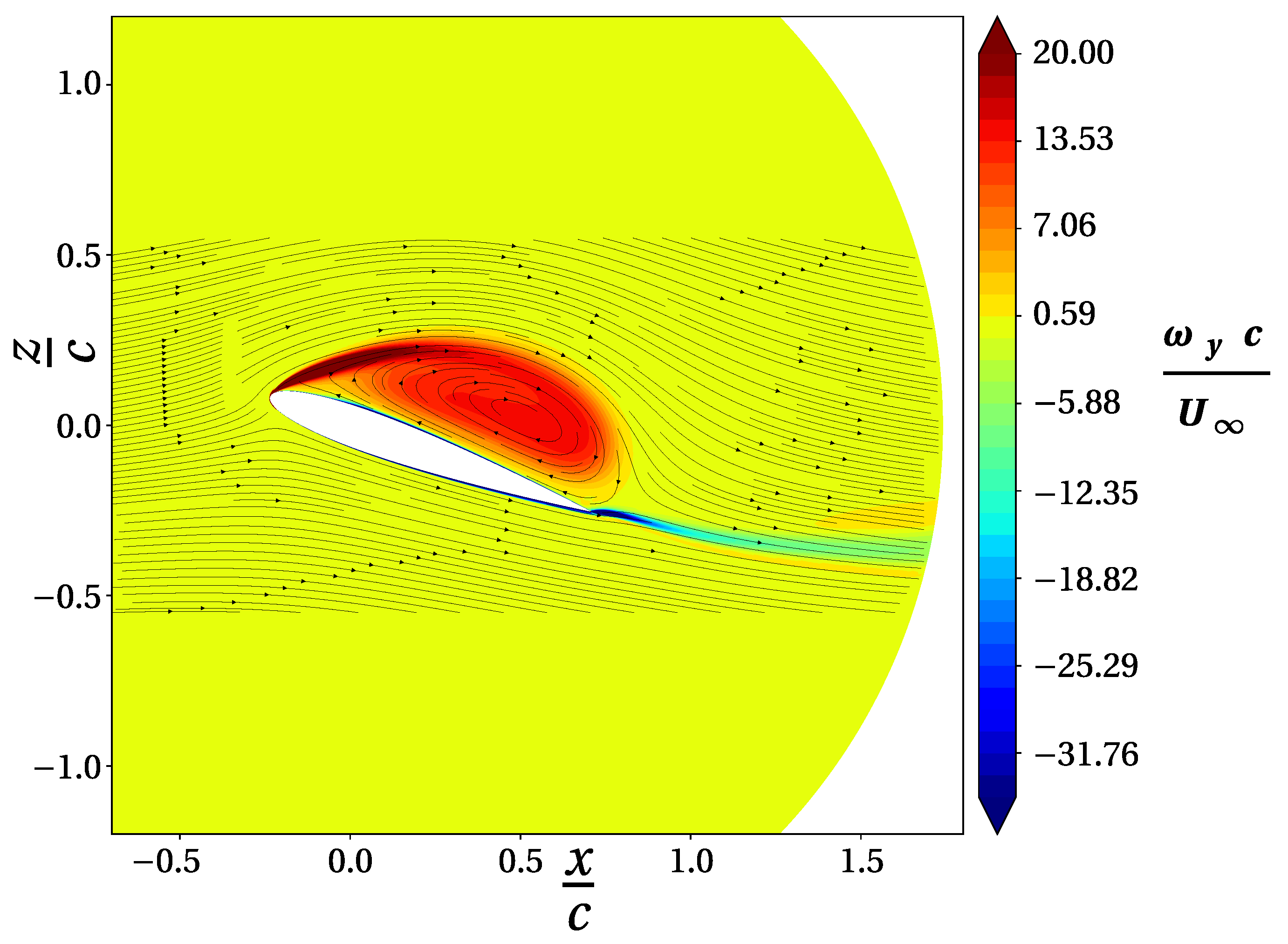
Figure 4.
Comparison of the aerodynamic coefficients as a function of the angle of attack. Lift (a), drag (b) and moment (c) coefficients of the present model are plotted against the experiments from Lee and Gerontakos [43] (black dots). Computational results are obtained with two turbulence models: respectively, Spalart-Allmaras with Edwards modification (green dots) and Menter SST (2003) (red dots). Plots report the average of the values referred to the last 3 pitching cycles.

Figure 5.
Maximum value of as a function of time for the case study configuration. The values of the last cycle are reported against the physical time, which is non-dimensionalised with the pitching period, T, and shifted to cover a normalised scale bar.
Figure 5.
Maximum value of as a function of time for the case study configuration. The values of the last cycle are reported against the physical time, which is non-dimensionalised with the pitching period, T, and shifted to cover a normalised scale bar.

Figure 6.
Lift (a), drag (b) and moment (c) coefficients as a function of the angle of attack throughout the the flow evolution of the test case and corresponding flow contours. Flow field distributions depict non-dimensional curl field (y component) superimposed with flow streamlines.
Figure 6.
Lift (a), drag (b) and moment (c) coefficients as a function of the angle of attack throughout the the flow evolution of the test case and corresponding flow contours. Flow field distributions depict non-dimensional curl field (y component) superimposed with flow streamlines.

Figure 7.
Energies (blue) and corresponding cumulative sums (red) as a function of wave mode (a,c,e). The plots refer to the three filter sizes used for the velocity field decomposition, respectively: (a,b) , (c,d) , (e,f) . The modes recovering the 99% of the signal are coupled and corresponding pairs are represented as dots in the spectrum plots (b,d,f): size and colour correspond to the time correlation of the two single modes.
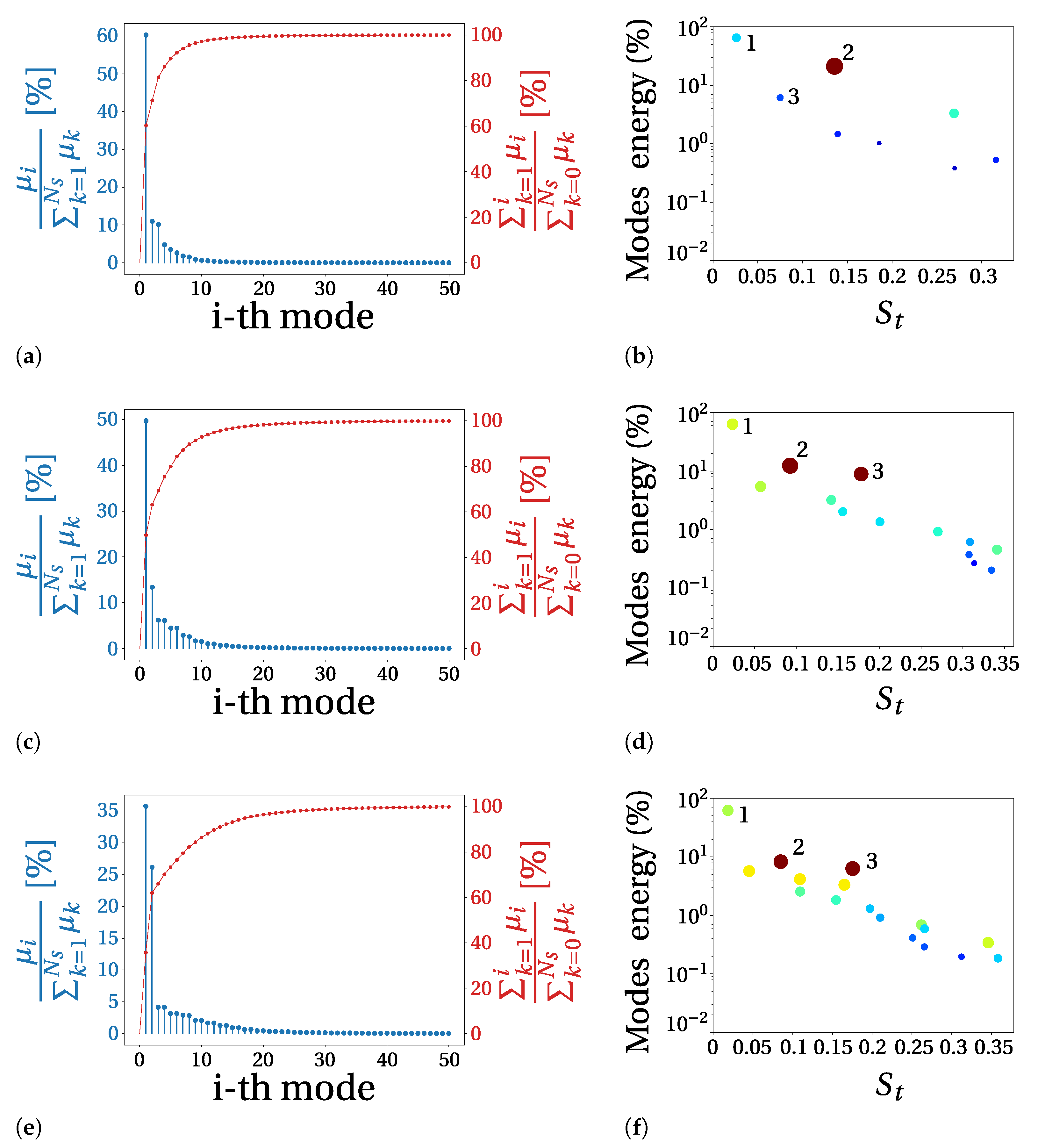
Figure 8.
Temporal behaviour of the third pair () of the velocity field decomposition, corresponding to the three filter sizes used, respectively from the left: (a,b) , (c,d) , (e,f) . Plots depict, respectively, the Power Spectral Density of the coupled time coefficients (a,c,e) and the phase portraits of the time coefficients of the two single modes (b,d,f).

Figure 9.
Spatial coherence of the third pair of the velocity field decomposition, corresponding to the three filter sizes used, respectively from the left: (a,b) , (c,d) , (e,f) . The contours depict the coherent structures respectively of (a,c,e) and (b,d,f) and should be intended as connected with the w component of the velocity vector.

Figure 10.
SPOD spectrum of the pressure field decomposition, for the three sizes of filter used: (a) , (b) and (c) . Size and colour of the dots correspond to the time correlation of the two single modes.
Figure 10.
SPOD spectrum of the pressure field decomposition, for the three sizes of filter used: (a) , (b) and (c) . Size and colour of the dots correspond to the time correlation of the two single modes.
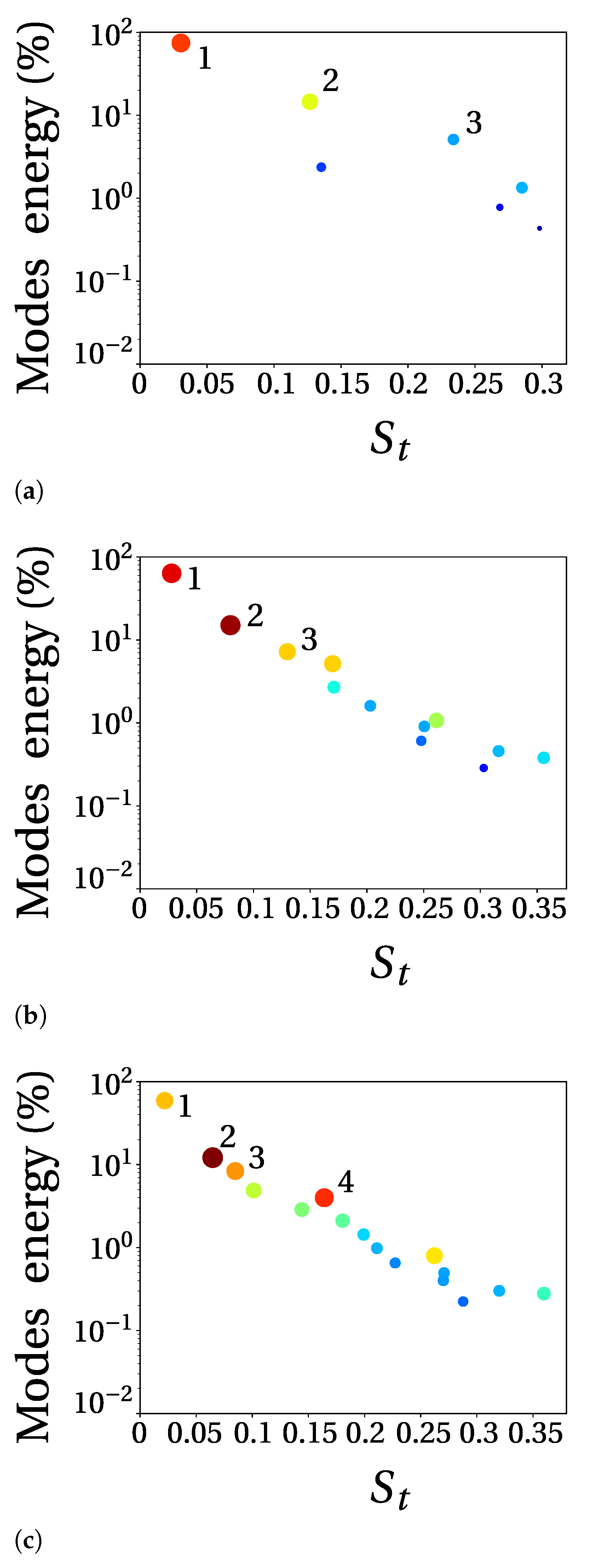
Figure 11.
Comparison between the coherent structure from velocity decomposition with filter width (a,b) and pressure decomposition with (c,d). Contours refer to the second pair, respectively (Figure 11a,c) and (b,d).
Figure 11.
Comparison between the coherent structure from velocity decomposition with filter width (a,b) and pressure decomposition with (c,d). Contours refer to the second pair, respectively (Figure 11a,c) and (b,d).

Figure 12.
Aerodynamic coefficients as a function of the angle of attack. The plots compare between the original solution from TAU (red) and values recomputed from a reconstruction of the pressure field with a number of modes that recovers the 95% of the original data (blue). The reported values refer, respectively, to the reconstruction from a POD decomposition (filter width ) (a,c,e) and to the reconstruction from a SPOD decomposition () (b,d,f). Reconstructed values do not include the contribution of viscous forces.
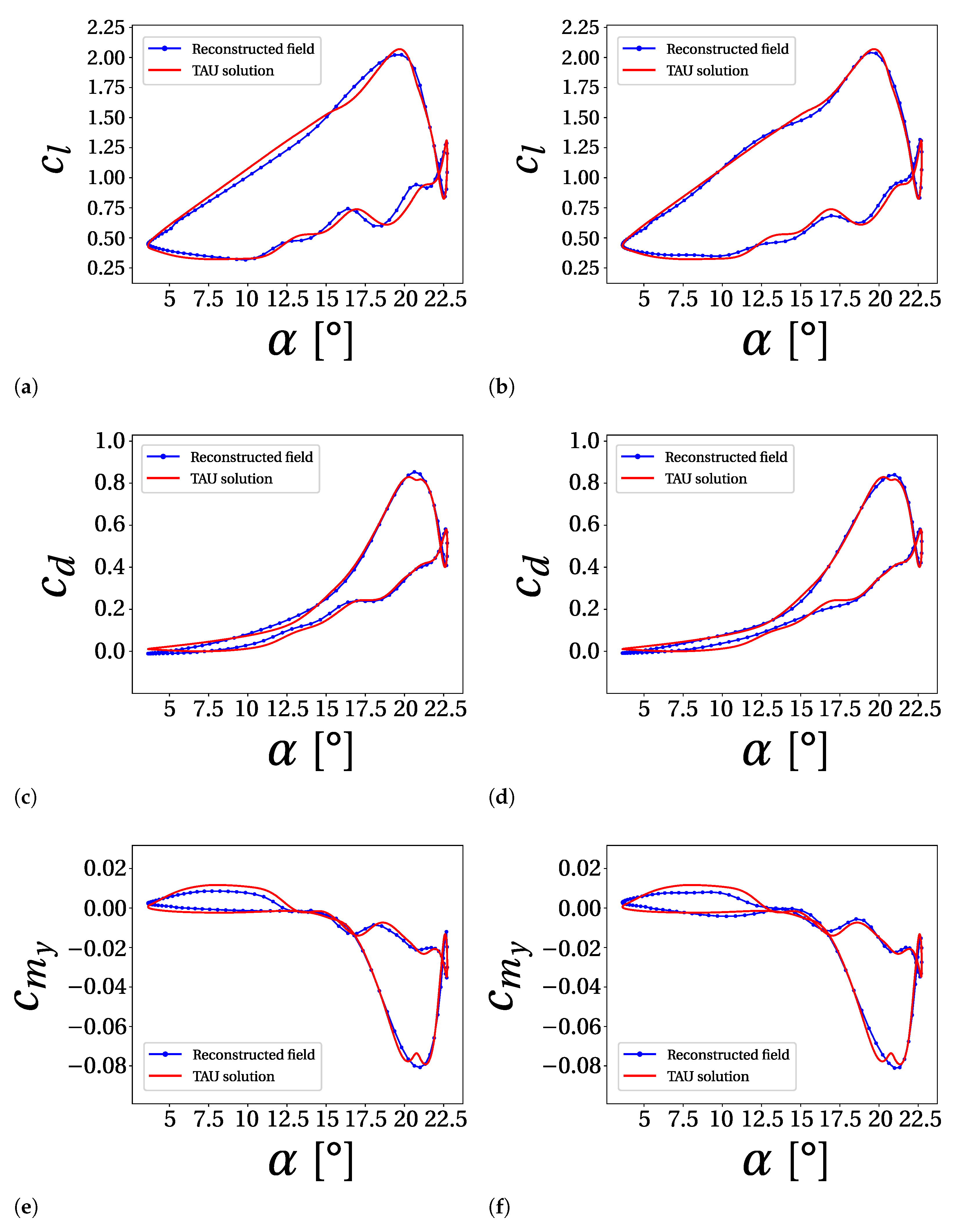

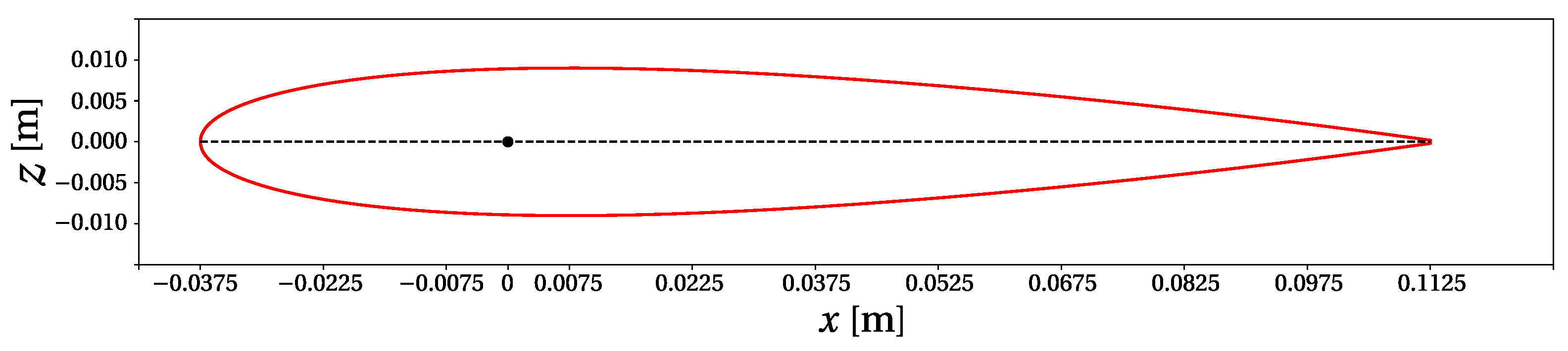
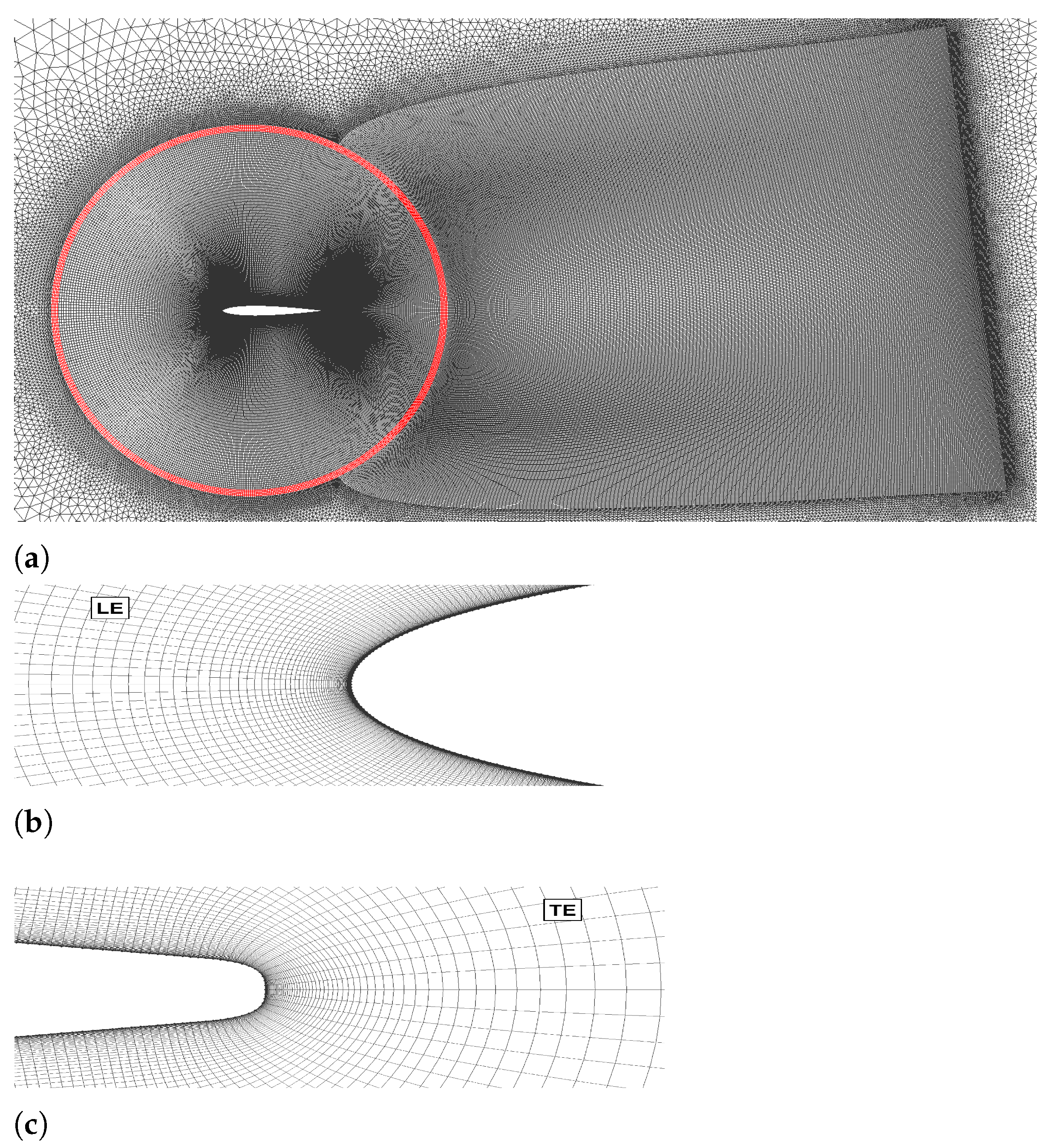
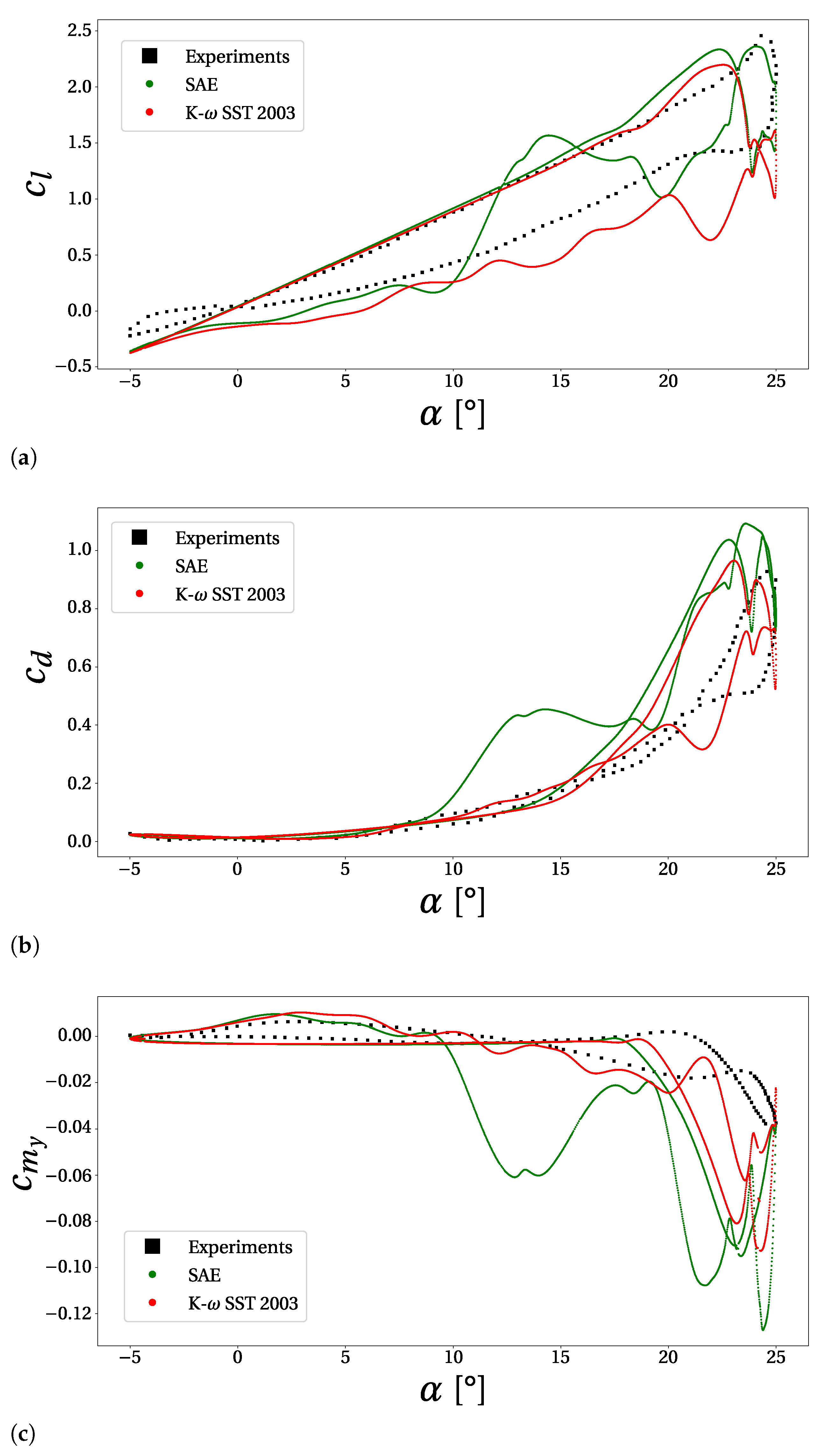
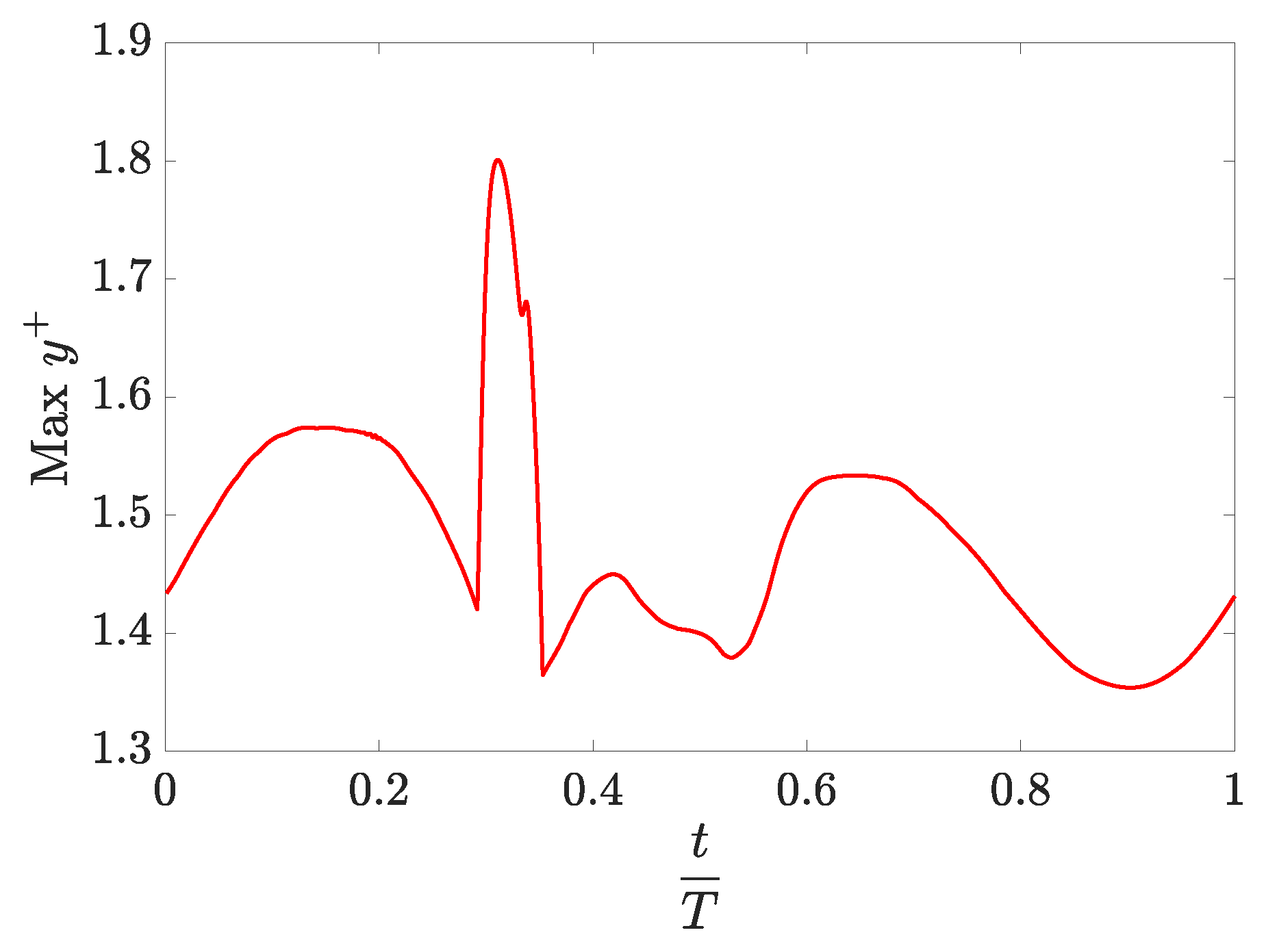
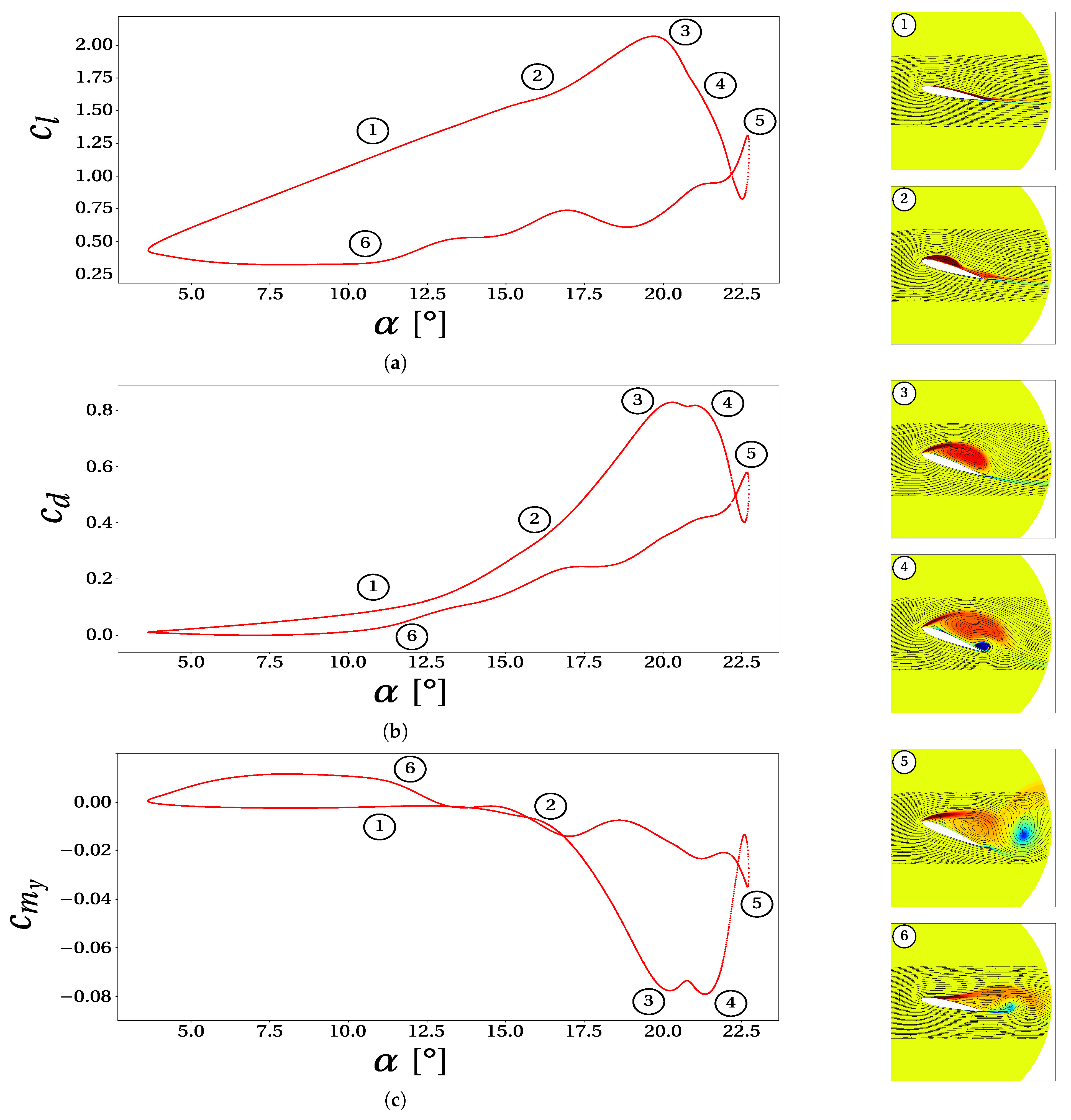
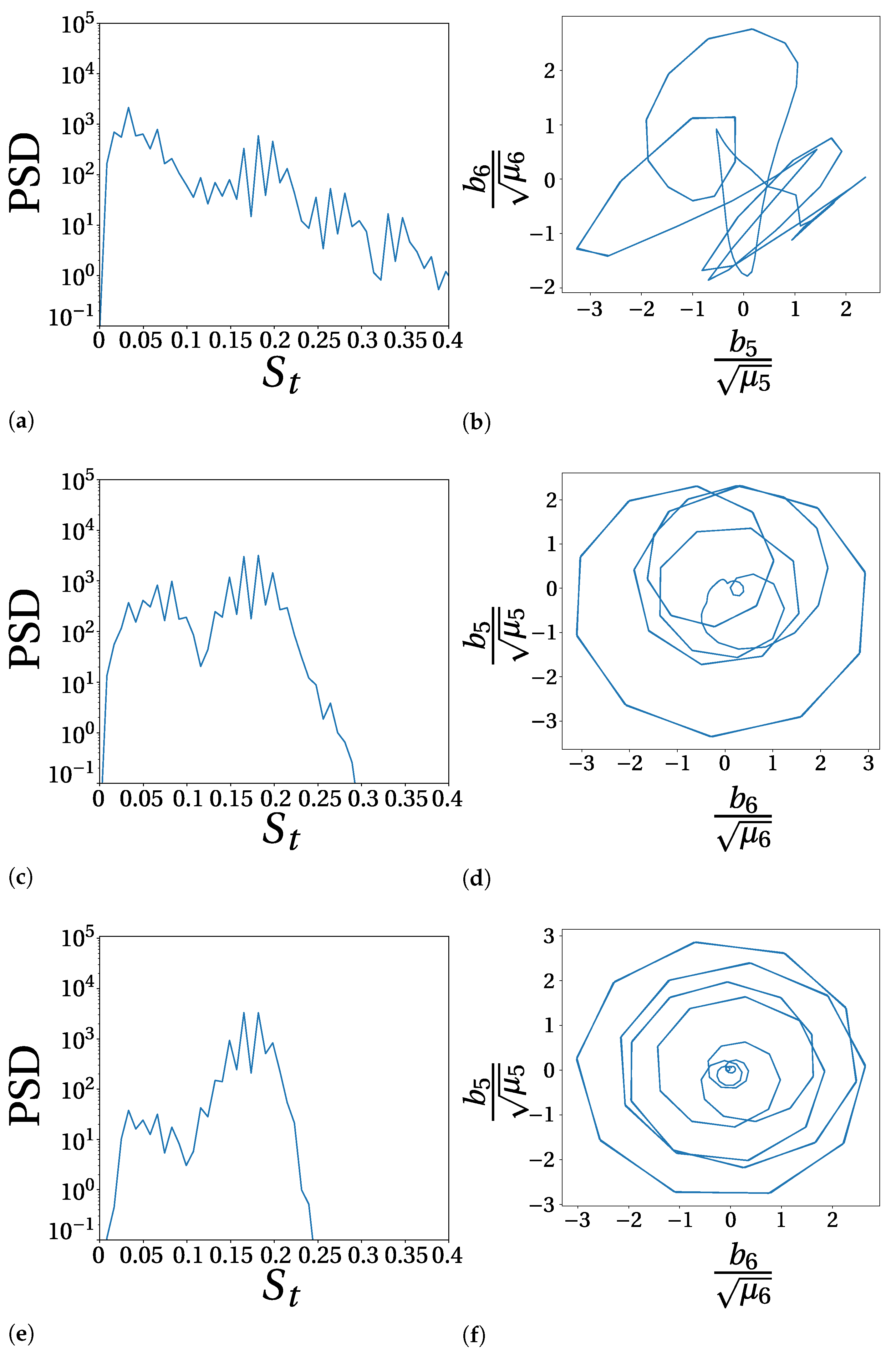
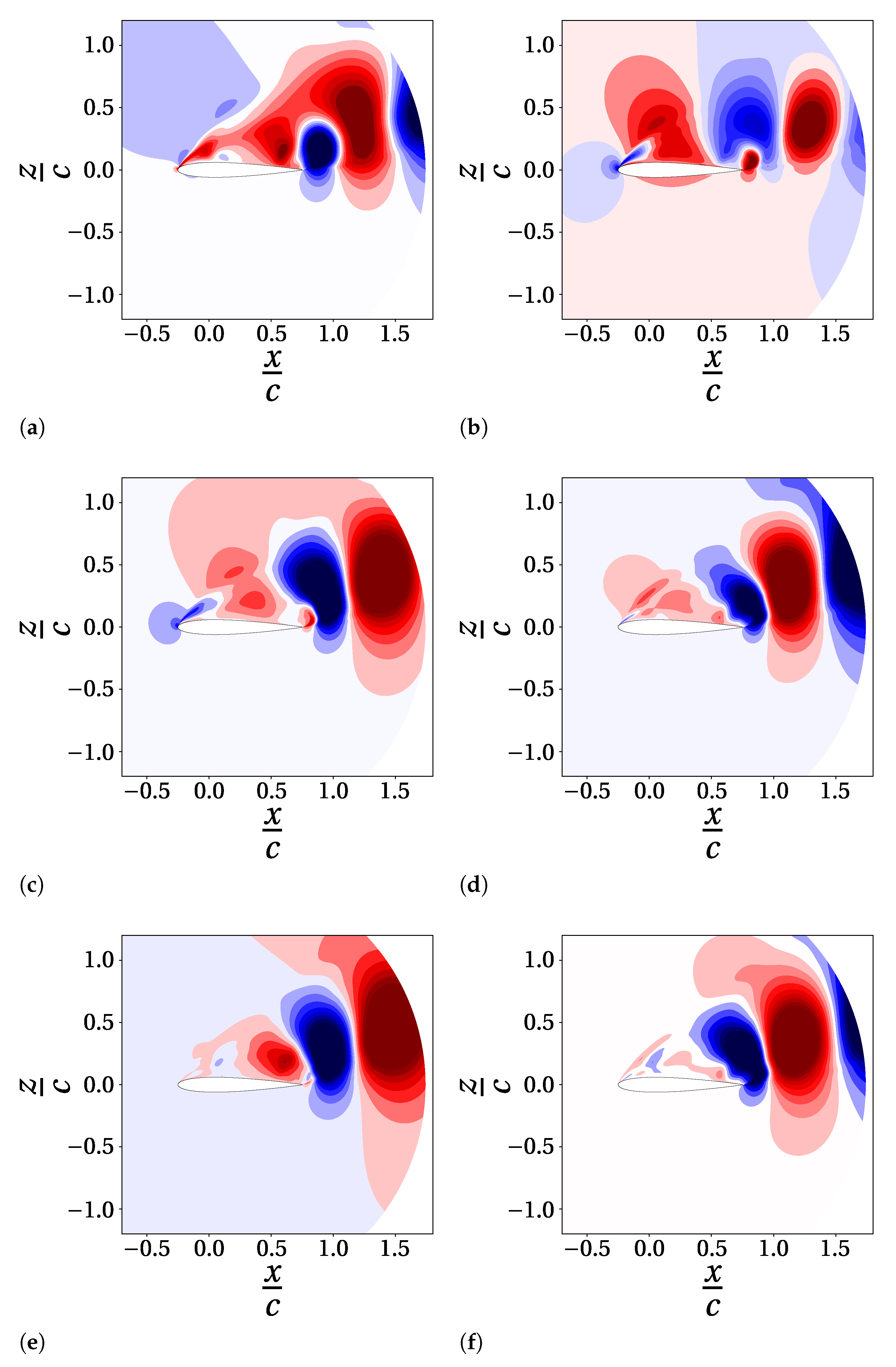
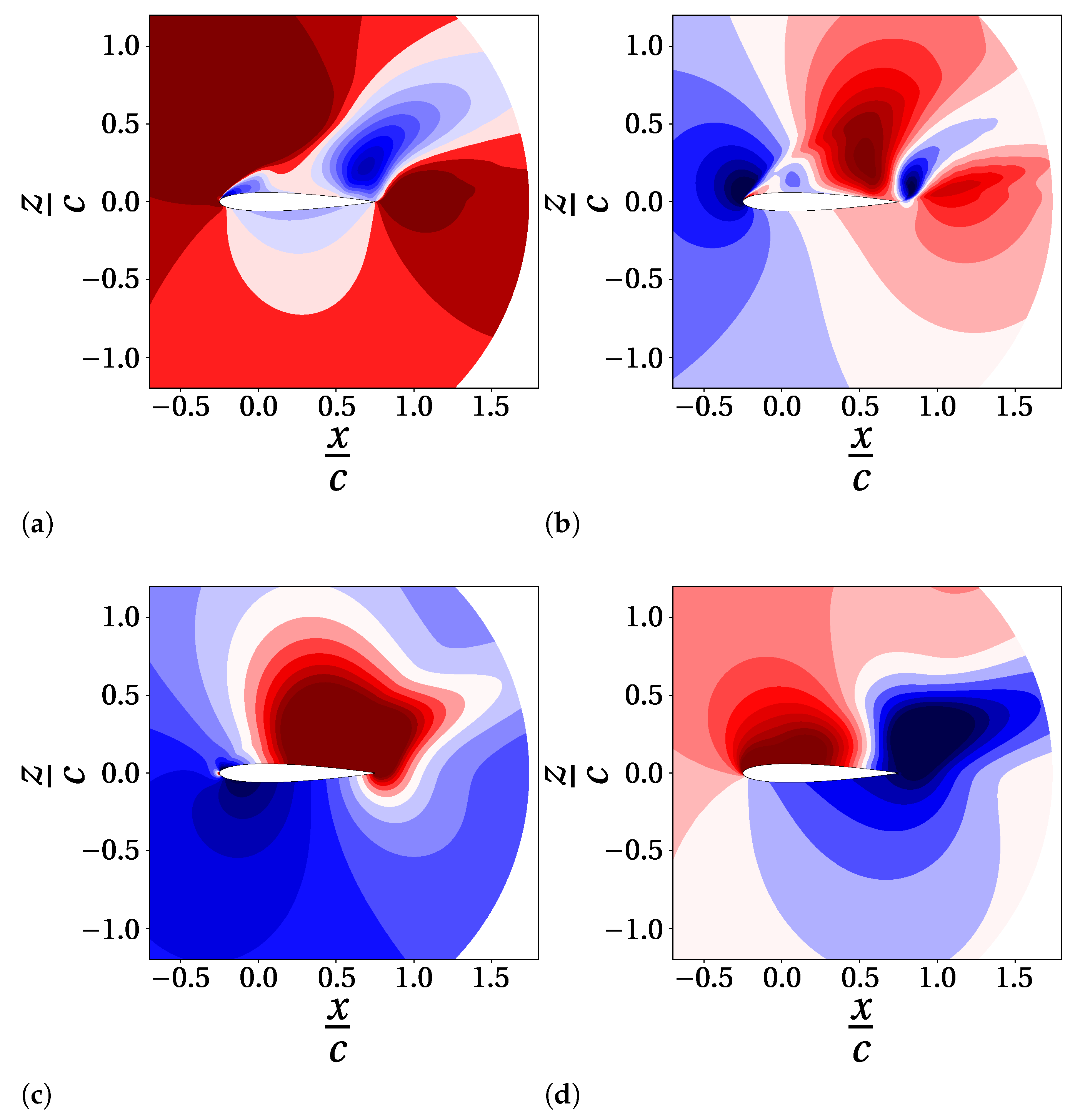
Table 1.
Flow conditions employed for simulations.
| Parameter | Symbol | Exp. Setup [12] | Case Study Setup |
|---|---|---|---|
| Mean angle of attack [] | 10 | 13.18 | |
| Pitch amplitude [] | 15 | 9.55 | |
| Reduced frequency | k | 0.1 | 0.135 |
| Pitching angular frequency [rad/s] | 18.67 | 275 | |
| Free stream velocity [m/s] | 14 | 152.73 | |
| Reynolds number | 1.35·105 | 1.57·106 |
Publisher’s Note: MDPI stays neutral with regard to jurisdictional claims in published maps and institutional affiliations. |
© 2021 by the authors. Licensee MDPI, Basel, Switzerland. This article is an open access article distributed under the terms and conditions of the Creative Commons Attribution (CC BY) license (http://creativecommons.org/licenses/by/4.0/).
Share and Cite
MDPI and ACS Style
Avanzi, F.; De Vanna, F.; Ruan, Y.; Benini, E. Design-Assisted of Pitching Aerofoils through Enhanced Identification of Coherent Flow Structures. Designs 2021, 5, 11. https://0-doi-org.brum.beds.ac.uk/10.3390/designs5010011
AMA Style
Avanzi F, De Vanna F, Ruan Y, Benini E. Design-Assisted of Pitching Aerofoils through Enhanced Identification of Coherent Flow Structures. Designs. 2021; 5(1):11. https://0-doi-org.brum.beds.ac.uk/10.3390/designs5010011
Chicago/Turabian StyleAvanzi, Filippo, Francesco De Vanna, Yin Ruan, and Ernesto Benini. 2021. "Design-Assisted of Pitching Aerofoils through Enhanced Identification of Coherent Flow Structures" Designs 5, no. 1: 11. https://0-doi-org.brum.beds.ac.uk/10.3390/designs5010011