Finding Multiple Equilibria for Raiffa–Kalai–Smorodinsky and Nash Bargaining Equilibria in Electricity Markets: A Bilateral Contract Model

Abstract

In a deregulated market, energy can be exchanged like a commodity and the market agents including generators, distributors, and the end consumers can trade energy independently settling the price, volume, and the supply terms. Bilateral contracts (BCs) have been applied to hedge against price volatility in the electricity spot market. This work introduces a model to find all solutions for the equilibria implementing the Raiffa–Kalai–Smorodinski (RKS) and the Nash Bargaining Solution (NBS) approaches in an electricity market based on BCs. It is based on creating “holes” around an existing equilibrium within the feasibility set, yielding a new (smaller) feasibility set at each iteration. This research has two players: a generation company (GC) and an electricity supplier company (ESC), aiming to achieve the highest profit for each of them. The results present all possible RKS and NBS, in addition to showing all assigned energies for a case study at different time frames. The multiple equilibria solutions allow the ESC and the GC to apply different strategies knowing that they can still achieve an optimal solution.

1. Introduction

The deregulated energy sector permits the actors to interconnect in optimal trading strategies by bilateral contracts (BCs) or the spot market. Electricity acquired by a BC can be resold on the spot market and electricity bought in the spot market can be used to accomplish BC obligations [1,2]. BCs in a deregulated market secure delivery of a certain amount of electricity at agreed upon prices while the spot market can have very volatile prices. Nevertheless, negotiation procedures present a main defiance to optimize the agents’ revenues given the possible buying and selling decision alternatives.

BCs are often used to reduce uncertainty and volatility risks of spot prices. High demand, for instance, results in a higher increase in the price of the electricity. Once the spot market prices have uncertainties, they can then have higher or lower prices than the forecasted ones, and the bilateral contracts then become an essential technique to support and mitigate risks.

This type of contract is negotiated based on the expected long-run price averages. Even though the contract can be applied to avoid risk, spot bidding may also allow the opportunity for higher profits to the players. High prices in the spot market favor the generation company (GC) to increase sales in this market reducing deliveries under BC. Concurrently, it is beneficial for the electricity supply company (ESC) to reduce purchase from the spot market increasing the contract deliveries [3]. The participating actors then need to administer the mix of the spot market transactions and the BCs seeking profit maximization.

1.1. Literature Review

Previous works analyzed the relation among BCs and ESCs as well as policies to deal with price risk [4,5,6]. They = applied the concept of efficient frontier as a tool to identify the preferred contract portfolio while also introducing methodologies to implement bidding strategies for electricity producers. Moreover, policies for market generation bidding, where the mean-variance criteria and uncertainty tools are implemented, have been developed in addition to binary expansion approaches [7,8,9,10].

Multiple equilibria solutions have already been studied in fields like game theory and microeconomics [11,12,13,14]. The problem of the tragedy of the commons has yielded multiple equilibria in a Markov model where every individual has the incentive to consume a resource at the expense of every other individual without excluding anyone from consuming. It results in overconsumption, under investment, and, ultimately, depletion of the resource. The authors in [12] reconsider the claim that one can solve, or at least mitigate, the tragedy of the commons with a play in nonlinear strategies.

Multiple Nash equilibria have also been analyzed applying machine learning to a multi-area network resembling the Scandinavian power system using the Nikaido–Isoda function [13]. The authors aim to find multiple Nash equilibria by the Gröbner basis methodology proposing a machine learning framework to train agents to replicate the single player results. Finally, the pure Nash equilibria in a pool-based electricity market with stochastic demand has also been studied in [14]. The set of all Nash equilibria is obtained along with the market clearing prices and assigned energies by the independent system operator (ISO).

In particular, for the electricity market, there are works regarding not only Nash equilibrium bidding strategies in a bilateral market for one time period, but also numerical solutions to Nash–Cournot equilibria in coupled constraints [15,16,17,18]. The work in [15] shows an analysis of the Nash equilibrium presented in [16], where the required conditions for Nash equilibrium bidding strategy based on a generic cost matrix and the loads willingness to pay vector are developed. Nevertheless, [15] shows that, depending on the assumptions, it is possible that the previously shown Nash equilibria model considered in [16] is inconsistent with the definition of Nash equilibrium. The works in [17,18] obtain numerical solutions to Nash–Cournot equilibria based on a relaxation algorithm and the Nikaido–Isoda function for electricity markets presenting a case for the IEEE 30-bus system.

Long-term Nash equilibria in electricity markets and the computation of all Nash equilibria in a multiplayer game have also been studied [19,20]. A methodology has already been developed to find plausible long-term Nash equilibria in a pool-based electricity market applying an iterative market Nash equilibrium model where the companies decide upon their offer strategies [19]. Moreover, the computation of all Nash equilibria in a multiplayer game in electricity markets has been obtained applying polynomial equations and the payoff matrix for the players [20]. In the latter work, the authors decompose the game converting the Nash equilibrium to a polynomial system of equations, obtaining all the solutions to the system of equations besides verifying if the obtained solutions satisfy the inequality constraints.

Studies where equilibria of electricity markets are evaluated, taking into account peer-to-peer energy exchanges or the storage of energy by the operators, have also been analyzed [21,22]. A network of prosumers has been considered having price differentiation in their preferences and considering two cases where a centralized market design was used as a benchmark or a distributed peer-to-peer market design is developed [21]. Discussions where other solutions for the peer-to-peer market design may exist and works related to the electricity storage have already been presented as a generalized Nash equilibrium for the problem, illustrating the approach for a three-node network and the IEEE 14-bus network [21,22]. The problem of electricity market equilibria with storage modeling was also analyzed in [22]. It is considered that the spot market trading of electricity includes different players like storage operators, producers, and consumers, where storage devices allow for shifting proceed electricity from one time period to a later one.

Relevant works have also been published regarding market equilibrium models applied to electricity markets [23,24]. The formulation of the electricity market applying equilibrium models as well as the distinction of these models related to the economics and commercial aspects of the problem have been addressed [23]. The implementation of electricity market equilibrium methods to assess not only the economic benefits of transmission expansions for market environments, and forward and spot markets, but short-term power system security has also been taken into account considering techniques to compute the electricity market equilibrium problems [24].

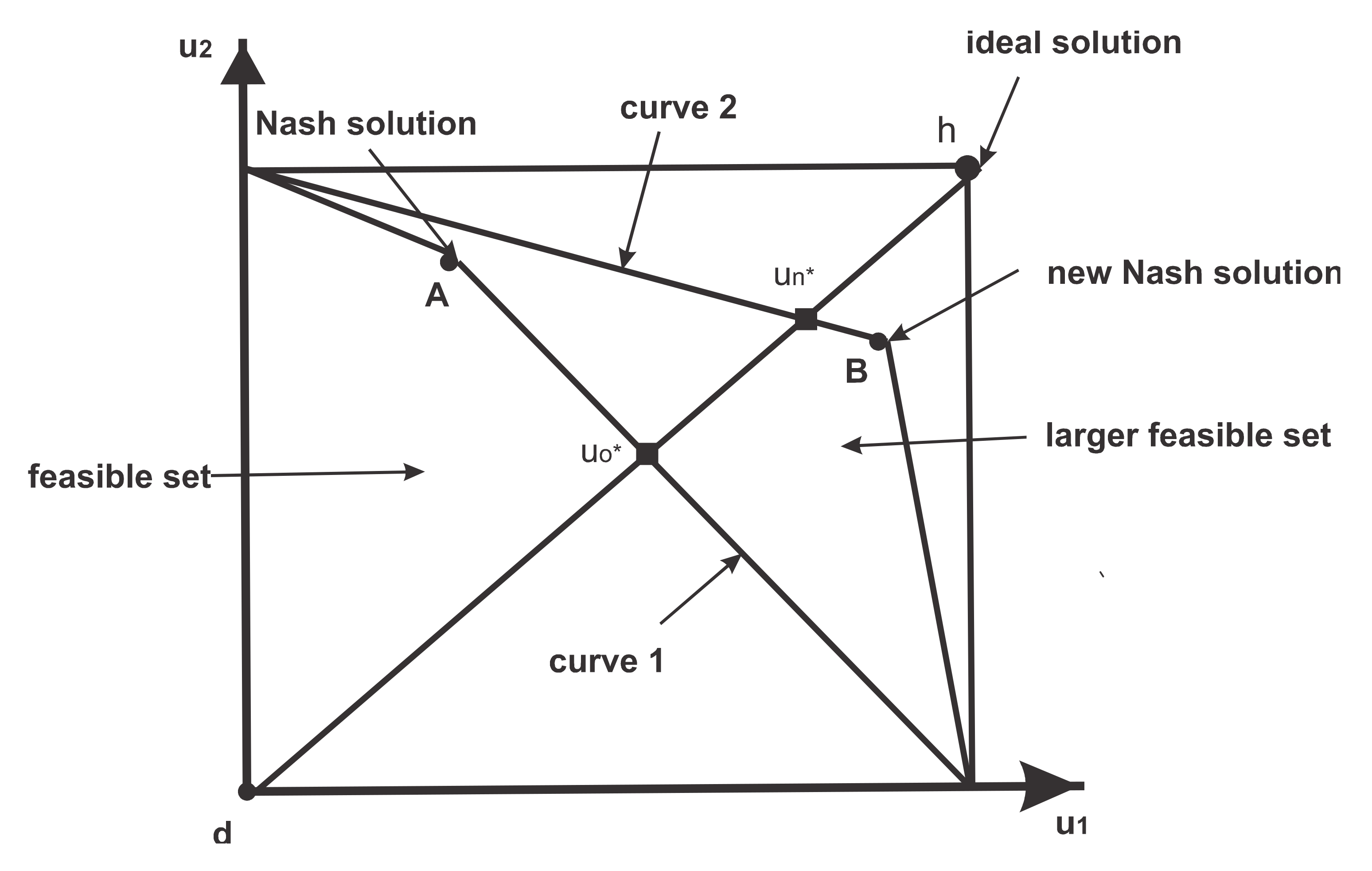
Apart from the previously mentioned works on Nash equilibrium, there are very few works dealing with bargaining solutions in electricity markets, other than the seminal paper [2] by Palamarchuk. He was the first to propose a different approach achieving a deal uniformly advantageous for both actors, the ESC and the BC. Moreover, it implements the Nash bargaining solution (NBS) to attain the relative concession to be made by both actors. Extending the work of Palamarchuk, another work has shown that a better outcome can be obtained implementing the Raiffa–Kalai–Smorodinsky (RKS) bargaining solution [25].

In this respect, one of the first works to show the connections between the NBS and the RKS is [26], where both approaches are compared for the supply chain contract negotiation problem, indicating that the RKS outperforms the NBS. In addition, Ruusunen [27] presents barter contracts in energy exchange between independent power companies, using a game-theoretic approach based on the NBS. An automated negotiation procedure for peer-to-peer electricity trading is developed in [28], based on the well-known Rubinstein alternating offers protocol. It constructs a Pareto frontier where both NBS and RKS are represented. Another bargaining model for the economic dispatch problem with demand response is shown in [29], using the RKS. The authors formulate a wholesale price negotiation problem between the generation company and multiple utility companies. Since the negotiation problem between the generation company and multiple utility companies is a bargaining problem, the RBS is applied to achieve the optimal bargaining outcome. A similar framework using the RKS is proposed in [30] in a smart grid, for an electricity market, which consists of a generation company, multiple electric utility companies, and consumers.

1.2. Main Contributions

The models proposed in this work aim to find a compromise solution, instead of finding a traditional non-cooperative equilibrium (Nash), as shown in most of the previously described works [1,3,4,5,6,7,8,10,11,12,13,14,15,16,17,18,19,20,21,22,23,24]. This research extends the findings of [25], showing that multiple solutions can be obtained when applying the NBS and the RKS for different values of the contract volume. To the best of our knowledge, there has been no other work showing all possible bargaining solutions in an electricity market context, describing the advantages for the players regarding the issue of knowing these different solutions within a timeframe. The advantage of being able to discern between various solutions lies in the possibility of buying or selling more energy in the spot market and using BC contracts depending on the prices of the market, as will be explained in the “Case Study” section. Therefore, the research gap relies on the fact that multiple solutions for the NBS and the RKS bargaining problems have not been analyzed yet in relation to electricity markets composed of both spot market and BC contracts.

The main contributions of this work can be considered the following ones:

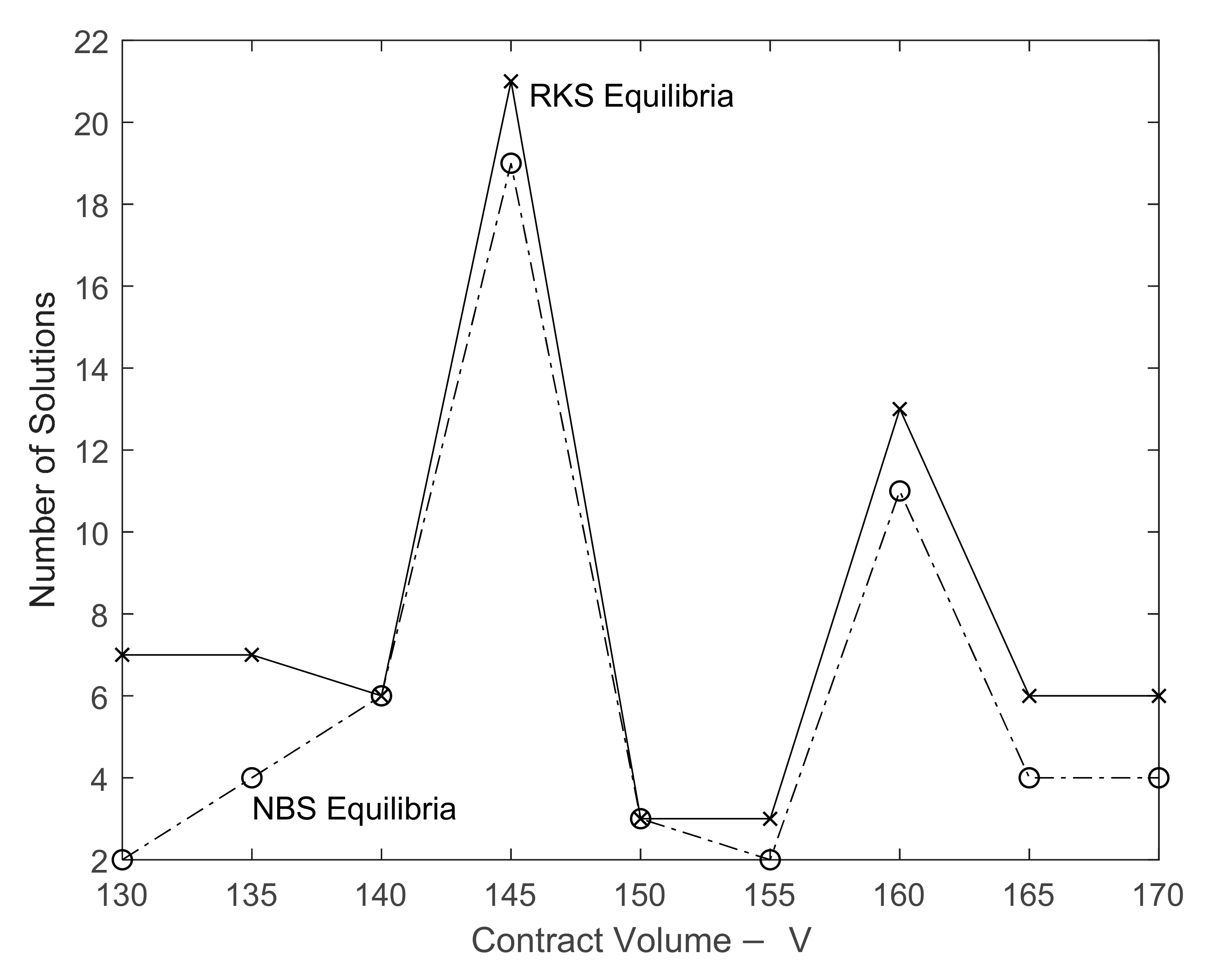
• the obtention of all multiple solutions when implementing the Nash bargaining (NB) and the Raiffa–Kalai–Smorodinsky (RKS) methods for an energy BC problem varying the values of the contract volumes for different time frames;
• comparisons of the solutions obtained when applying the NBS and the RKS methods for the considered BC problem in the electricity market; and
• description of the flexibilities the players can have to achieve the optimal solution in any of the NBS or the RKS applied approaches due to the existence of the multiple equilibria.

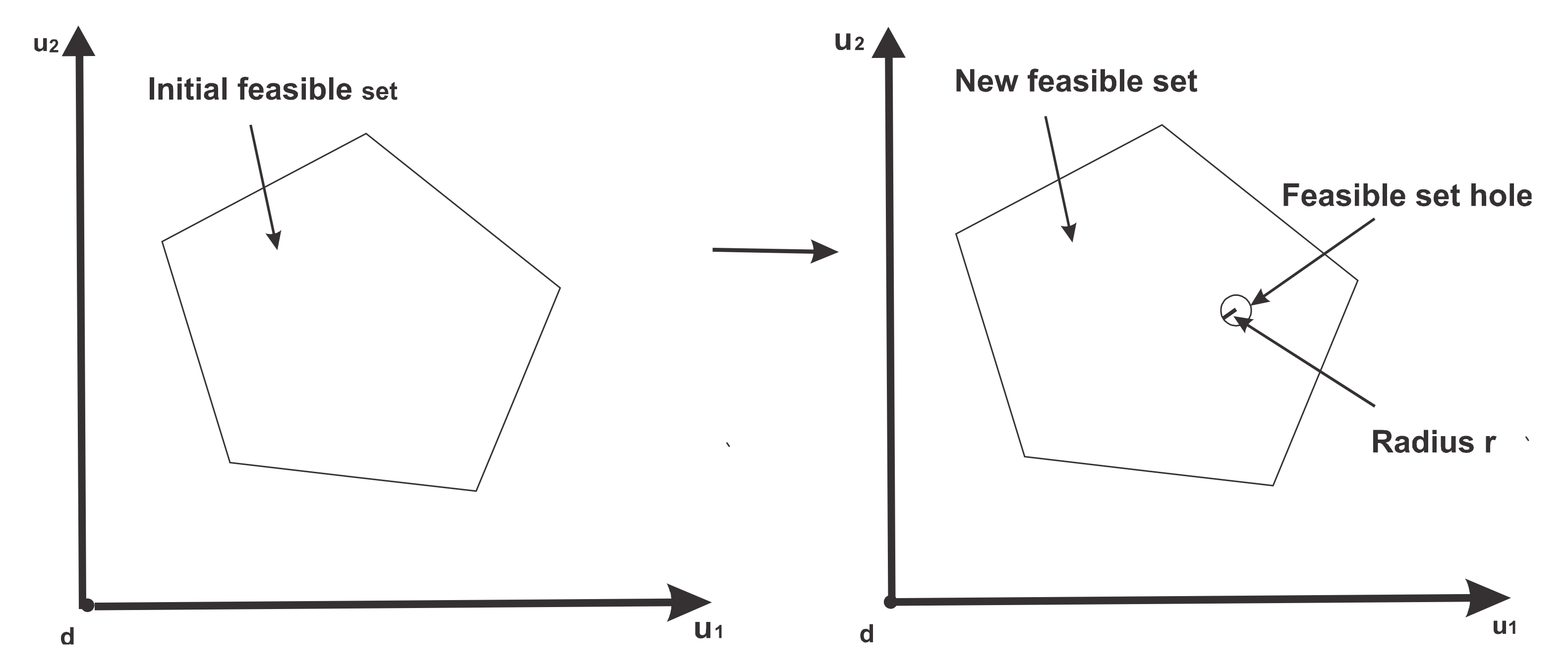
This paper implements the technique of creating a “hole” related to the already achieved solution in the feasible set (resulting in new feasible sets) to obtain all the optimal solutions [14]. The game assumes the existence of two players, an ESC and a GC, aiming to acquire a compromise approach implementing either the NBS or the RKS equilibrium. The input dataset includes the spot price scenarios and the demand for the end customers besides the production cost functions, the electricity generation limits, and the deliveries under the BCs. The methodology is implemented for different values of contract volumes in different time frames showing the total number of optimal solutions for the RKS and the NBS equilibria found. Therefore, the main innovation of this paper is the implementation of a model to obtain all the NBS and RKS equilibria for a BC problem in an electricity market. No other paper at this time, to our knowledge, has tried to achieve these results.

The paper is organized as follows. The background for the developed RKS and NBS problems is presented in Section 2 besides the analytical models applied for the bilateral contracts. Additionally, the methodology to obtain all optimal solutions is presented. The results when implementing the developed approach is shown in Section 3 obtaining the multiple equilibria for NBS and the RKS procedures. The conclusions are stated in Section 4.

2. Materials and Methods

The proposed model to obtain the multiple solutions for the NBS and the RKS is explained in the next subsections as well as the implemented compromise approach among the players. The BC model applied is also presented.

2.1. Multiple Equilibria Raiffa–Kalai–Smorodinsky and Nash Bargaining Solutions

In order to achieve either a RKS or a NBS in a cooperative game, the players aim to find an agreement favorable for all players. A structure to reach a solution for a bargaining problem was proposed by Nash where a feasible solution was attained as the result. A bargaining result is an equilibrium allocation satisfying the players giving them no grounds to negotiate any further.

The structure proposed by Nash included the axioms called symmetry (SYM), weak Pareto optimality (WPO), scale invariance (SI), and independence of irrelevant alternatives (IIA) [16]. Afterwards, the IIA axiom was substituted with a monotonicity axiom, yielding another structure where the solution was directed to ideal parties payoff related to the maximum likely payment that one actor could attain independently, this being called the RKS solution [31,32]. This concept was a critique of the Nash approach as the NBS could give a worse result even if it had a larger feasible set.

When analyzing Figure 1, one can observe the RKS and the NBS. The obtained NBS when the viable region limited by Curve 1 is represented by point A. When the feasible set is represented by Curve 2, the new NBS solution is given by point B, making player 2 worse off, even though Curve 2 has a larger feasible set than Curve 1. For the RKS approach, the obtained solution achieved when the feasible set is limited by Curve 1 is represented by point $u_0^{*}$; whereas, if the viable region is given by Curve 2, point $u_n^{*}$ represents the new solution, both players will better off if the RKS technique is implemented (Figure 1). Thus, the RKS bargaining solution is a Pareto optimal point in the line from d to the ideal solution, h [31,32].

Finally, a bigger viable region having the same ideal result represented by point h, in Figure 1, achieves a bargaining result better (or no worse) for all actors when implementing the RKS approach. Therefore, the RKS bargaining result is a Pareto optimal point where both actors obtain an equal proportion of their potential utility benefits estimated by [28,29]:

$$\frac{u_{n1}^{*}-d_1}{u_{n2}^{*}-d_2}=\frac{h_1-d_1}{h_2-d_2}$$

(1)

Further analysis can be made to find all the RKS and the NBS equilibria for the BC problem in electricity markets. This work proposes then to find all RKS and NBS equilibria where two players are considered, a GC and an ESC. The applied methodology is represented by Figure 2, where an initial feasible set is considered.

Whenever a solution is obtained, either for the RKS or the NBS problem, a “hole” of radius r related to that solution is made in the feasible set, resulting in a new feasible set. A new solution, taking into account a new reduced feasible set, is obtained. The procedure continues until the newly obtained solution, either applying the RKS or the NBS approaches, results in a new value for the objective function which is worse than the initial one when adding an extra constraint related to the hole. Certainly, the radius r in the hypersphere hole has to be very small and the new result must not belong to the border of the hypersphere hole, otherwise another new solution could be missed [14].

2.2. Bilateral Contract Scheduling

In this work, scheduling refers to the quantity of electricity being conveyed at each interval t during the contract period [2]. The parties, either the GC or the ESC, schedule the electricity deliveries to maximize their profits having forecasted the electricity prices in the spot market. Therefore, the electricity prices in the spot market are random variables [33].

In order to compare our results with previous ones [2,25] we define:

Type I: The buyer (ESC) aims to maximize its predicted profit, called S₁, determining the electricity quantity to be conveyed by the BC, at each time interval t. The supplier (GC) must assure the electricity to be dispatched in agreement with the buyer’s demands.

Type II: The supplier (GC) aims to maximize its predicted profit, called S₂, determining the electricity quantity to be sold respecting the contract at each time interval t. The buyer (ESC) has to accept the required electricity in agreement with the GC maximizing the GC predicted profit.

The following equations are then applied to solve contract Types I and II [2,25].

For the Type I contract, ESC’s profit (S₁) is evaluated by:

$$\underset{x_k^t,x_s^t,x_{ss}^t}{\max }{S}_1=E\left\{{\displaystyle \sum }_{t=1}^N\left[p_d^t(x_k^t+x_s^t)-p_s^{~t}{x}_s^{~t}+p_s^{~t}{x}_{ss}^t\right]-J\right\}$$

(2)

where E is the mathematical expectation symbol. Furthermore, J is the contract value, being a constant in this research, since the actors agree on a contract price in their BC. Moreover, $p_d^t$ and $p_s^{~t}$ represent the electricity price for the final consumers in the retail market at period t and the discrete level of the spot market price, respectively. Finally, $x_k^t,x_s^t,\mathrm{and}{x}_{ss}^t$ represent the quantity of electricity delivered under the BC and sold to end consumers, the quantity of electricity bought by the ESC in the spot market, and the quantity of electricity received by the ESC under the BC and sold in the spot market all at period t, respectively.

The aim to maximize the profit means to maximize the predicted sales revenue, R₁, in the spot and the retail markets:

$$\underset{x_k^t,x_s^t,x_{ss}^t}{\max }{R}_1=E\left\{{\displaystyle \sum }_{t=1}^N\left[p_d^t(x_k^t+x_s^t)-p_s^{~t}{x}_s^{~t}+p_s^{~t}{x}_{ss}^t\right]\right\}$$

(3)

subject to:

(a) the total contract volume:

$${\displaystyle \sum }_{t=1}^N\left(x_k^t+x_{ss}^t\right)=V$$

(4)

(b) the sales to end consumers:

$$\left(x_k^t+x_s^t\right)=x_d^t,t=1,\dots ,N$$

(5)

(c) the delivery quantity by the contract at time intervals:

$$x_{min}^t\le \left(x_k^t+x_{ss}^t\right)\le x_{max}^t,t=1,\dots ,N$$

(6)

(d) the non-negativity of variables:

$$x_k^t\ge 0,x_s^t\ge 0,x_{ss}^t\ge 0,t=1,\dots ,N$$

(7)

The ESC solves the problem (3)–(7) to schedule the electricity deliveries x^t, t = 1, …, N for the contract interval, it then takes it to the GC. The GC must agree to the supply electricity according to the schedule proposed by the ESC.

Regarding the contract of Type II, the GC maximizes its profit, S₂, concurrently trading in the spot and in the BC markets. The GC’s production cost function, $C_k^t\left(x_g^t\right)$, is given as a function of the electricity generation, $x_g^t$, and it is evaluated by the optimal unit commitment [3].

Regarding the contract of Type II, GC’s profit (S₂) can be given as:

$$\underset{x_c^t,x_{gs}^t,x_{gss}^t}{\max }{S}_2^{ }=E\left[{\displaystyle \sum }_{t=1}^N\left(p_s^{~t}{x}_{gss}^t-p_s^{~t}{x}_{gs}^t-C^t\left(x_c^t+x_{gss}^t+J\right)\right)\right]$$

(8)

where $p_s^{~t}$ represents the discrete level of the spot market price. Furthermore, $x_{gss}^t,x_{gs,}^t\mathrm{and}{x}_c^t$ represent the quantity of electricity produced by the GC and sold in the spot market, the quantity of electricity bought by the GC in the spot market being dispatched under the BC, and the quantity of electricity produced by the generation company (GC) and delivered under the BC all at period t, respectively.

Since J is constant, (8) is equivalent to:

$$\underset{x_c^t,x_{gs}^t,x_{gss}^t}{\max }{R}_2^{ }=E\left[{\displaystyle \sum }_{t=1}^N\left(p_s^{~t}{x}_{gss}^t-p_s^{~t}{x}_{gs}^t-C^t\left(x_c^t+x_{gss}^t\right)\right)\right]$$

(9)

subject to:

(a) the electricity generation at each interval:

$$x_{gmin}^t\le \left(x_c^t+x_{gss}^t\right)\le x_{gmax}^t,t=1,\dots ,N$$

(10)

(b) the delivery amount under the contract at individual intervals:

$$\left(x_c^t+x_{gs}^t\right)=x^t,t=1,\dots ,N$$

(11)

(c) the non-negativity of variables:

$$x_c^t\ge 0, x_{gs}^t\ge 0, x_{gss}^t\ge 0,t=1,\dots ,N$$

(12)

The Type I and II problems are solved applying a stochastic dynamic programming approach where an increment in the electricity distributed at a period means a decrement at the others [2,25]. Once (3)–(7) and (9)–(12) are solved, the maximum profits are evaluated and the compromise approach is applied achieving either the RKS or the NBS.

2.3. Raiffa–Kalai–Smorodinsky and Nash Bargaining Solutions for Bilateral Contract Scheduling

The advantage that a player has over the other one, by obeying the consigned schedule, can be mitigated implementing a compromise approach for BC scheduling. The implementation allows to determine the electricity deliveries achieving relative equal benefits to parties. Therefore, the actors, the Gc and the ESC, can schedule deliveries jointly or by a neutral third player.

When solving the compromise approach, the GC and the ESC schedule their deliveries separately. If the ESC schedules deliveries x^t, t = 1, …, N independently, it solves the problem (3)–(7) obtaining its maximum profit, $S_1^{*}$. Similarly, if the GC schedules the deliveries x^t, t = 1, …, N separately, it will not pursue the dispatch schedule given by the ESC. The compromise approach replaces constraint (11) in problem (9)–(12), with the following ones:

$${\displaystyle \sum }_{t=1}^N\left(x_c^t+x_{gs}^t\right)=V$$

(13)

and the quantity dispatched under the BC at the times t must obey:

$$x_{min}^t\le x_c^t+x_{gs}^t\le x_{max}^t,t=1,\dots ,N$$

(14)

In order to solve the RKS bargaining problem, the objective function aims to maximize the revenues of the parties being represented by [25]:

$$\begin{gathered} \max (R_1+R_2)= \\ \max \left\{{\displaystyle \sum }_{t=1}^N\left[{\left(p\right.}_d^t\left(x_k^t+x_s^t\right)-p_s^{~t}{x}_s^t+p_s^{~t}{x}_{ss}^t\right)\left]+ {\displaystyle \sum }_{t=1}^N\right[p_s^{~t}{x}_{gss}^t-p_s^{~t}{x}_{gs}^t-C^t\left(x_c^t+x_{gss}^t\right)]\right\} \end{gathered}$$

(15)

Adding the constraint related to the RKS solution:

$$\frac{E\left\{{\sum }_{t=1}^N\left[{\left(p\right.}_d^t\left(x_k^t+x_s^t\right)-p_s^{~t}{x}_s^t+p_s^{~t}{x}_{ss}^t\right)]\right\}-J^0}{E\left\{{\sum }_{t=1}^N\left[p_s^{~t}{x}_{gss}^t-p_s^{~t}{x}_{gs}^t-C^t\left(x_c^t+x_{gss}^t\right)\right]\right\}+J^0}=\frac{S_1^{*}}{S_2^{*}}$$

(16)

where $J^0$ represents the contract value given by the solution of the Types I and II contract problems, being given by $J^0=\frac{1}{2}\left(R_1^{*}+\left|R_2^{*}\right|\right)$.

The following conditions represented by (17)–(23) must also be satisfied:

$$E\left\{\sum _{t=1}^N\left[p_d^t\left(x_k^t+x_s^t\right)-p_s^{~t}{x}_s^t+p_s^{~t}{x}_{ss}^t\right]\right\}\ge \left|E\left\{{\displaystyle \sum }_{t=1}^N\left[p_s^{~t}{x}_{gss}^t-p_s^{~t}{x}_{gs}^t-C^t\left(x_c^t{x}_{gss}^t\right)\right]\right\}\right|$$

(17)

subject to:

(a) total contract volume:

$${\displaystyle \sum }_{t=1}^N\left(x_k^t+x_{ss}^t\right)=V$$

(18)

(b) sales to end consumers:

$$\left(x_k^t+x_s^t\right)=x_d^t,t=1,\dots ,N$$

(19)

(c) electricity generation at each interval:

$$x_{gmin}^t\le \left(x_c^t+x_{gss}^t\right)\le x_{gmax}^t,t=1,\dots ,N$$

(20)

(d) quantity of deliveries under contract at certain periods:

$$x_k^t+x_{ss}^t=x_c^t+x_{gs}^t,t=1,\dots ,N$$

(21)

$$x_{min}^t\le x_k^t+x_{ss}^t\le x_{max}^t,t=1,\dots ,N$$

(22)

(e) non-negativity of variables:

$$x_k^t\ge 0, x_s^t\ge 0, x_{ss}^t\ge 0, x_c^t\ge 0, x_{gs}^t\ge 0, x_{gss}^t\ge 0,t=1,\dots ,N$$

(23)

The number of the equilibria methodology implementing the NBS is compared with the results implementing the RKS just described. When implementing NBS, the objective function aims to minimize the concessions of each actor in the game, given by k ([2,25]):

$$k=\frac{\left(S_1^{*}-E\left\{{{\displaystyle \sum }}_{t=1}^N\left[p_d^t\left(x_k^t+x_s^t\right)-p_s^{~t}{x}_s^t+p_s^{~t}{x}_{ss}^t\right]\right\}+\frac{1}{2}\left(R_1^{*}+\left|R_2^{*}\right|\right)\right)}{S_1^{*}}$$

(24)

Furthermore, k is equal to:

$$k=\frac{\left(S_2^{*}+\left|E\left\{{{\displaystyle \sum }}_{t=1}^N\left[p_s^{~t}{x}_{gss}^t-p_s^{~t}{x}_{gs}^t-C^t\left(x_c^t{x}_{gss}^t\right)\right]\right\}\right|-\frac{1}{2}\left(R_1^{*}+\left|R_2^{*}\right|\right)\right)}{S_2^{*}}$$

(25)

Finally, once having obtained one of the solutions for the RKS and the NBS, solving Equations (15)–(23) and Equations (17)–(25), respectively, a hole of radius r centered in the obtained solution must be added to the feasible set, given by:

$${\displaystyle \sum }_{t=1}^3{(x_k^{e t}-x_k^{* t})}^2+ {(x_s^{e t}-x_s^{* t})}^2+ {(x_{ss}^{e t}-x_{ss}^{* t})}^2+{(x_c^{e t}-x_c^{* t})}^2+{(x_{gs}^{e t}-x_{gs}^{* t})}^2+{(x_{gss}^{e t}-x_{gss}^{* t})}^2 \ge r^2$$

(26)

where an optimal solution is given by the set ($x_k^{*t},x_s^{*t},x_{ss}^{*t,},x_c^{*t},x_{gs}^{*t},x_{gss}^{*t})$and the new one is given by $\left(x_k^{et},x_s^{e t},x_{ss}^{et,},x_c^{et},x_{gs}^{et},x_{gss}^{et}\right).$ The radius r in Equation (26) has to be small enough in order to not miss any result within the hypersphere hole, and the result must not belong to the border of the hypersphere hole [14]. Therefore, whenever a new optimal solution is found, where the objective function has a value equal to the previous one, a new constraint given by Equation (26) is added to the problem.

The following flowchart (i)–(v) summarizes the implementation of obtaining multiple equilibria for the RKS and the NBS.

(i)

Introduce the input data set of the model: spot price forecasts, electricity consumption by end customers, limits of electricity delivery, production cost functions, electricity generation limits. See

Table 1. Input data set for bilateral contract (BC) scheduling for the electricity supplier company (ESC).

Time Intervals	${\mathit{t}}_1$			${\mathit{t}}_2$			${\mathit{t}}_3$
Spot price forecasts obtained by ESC
spot price scenarios,$p_{sj}^t$ US$/MWh	10.0	10.4	10.8	11.0	11.2	11.8	11.0	11.4	11.8
probabilities of scenarios, ${\epsilon }_j^t$	0.1	0.8	0.1	0.3	0.5	0.2	0.2	0.4	0.4
electricity price for final consumers, US$/MWh	16			16			16
Constraints for the optimization problem
electricity consumption by final consumers, MWh	$x_d^1$			$x_d^2$			$x_d^3$
	9.8			11.4			14.5
limits on electricity dispatched under BC, MWh	$x_{min}^1$		$x_{max}^1$	$x_{min}^2$		$x_{max}^2$	$x_{min}^3$		$x_{max}^3$
	8		60	5		68	6		62

and

Table 2. Input data for BC scheduling for the generation company (GC).

Time Intervals	${\mathit{t}}_1$				${\mathit{t}}_2$				${\mathit{t}}_3$
Spot price forecasts made by GC
spot price scenarios,$p_{sj}^t$, US$/MWh	10.8	11.2		11.6	11.0	11.6		12.0	11.0	11.8		12.4
probabilities of scenarios, ${\epsilon }_j^t$	0.2	0.6		0.2	0.25	0.5		0.25	0.1	0.6		0.3
production cost functions, $C_k^t\left(x_g^t\right),$ US$	$8.4+1.4x_g^1+0.4\left(x_g^1\right)$2				$10.4+1.52x_g^2+0.44\left(x_g^2\right)$2				$11.2+1.4x_g^3+0.32\left(x_g^3\right)$2
Constraints for the optimization problem
electricity generation limits, MWh	$x_{gmin}^1$		$x_{gmax}^1$		$x_{gmin}^2$		$x_{gmax}^2$		$x_{gmin}^3$		$x_{gmax}^3$
	14.0		50.0		15.0		60.0		16.0		65.0
electricity dispatched under BC, MWh	15				68				62

[2,23].

(ii)

Solve the problem independently for the ESC and the GC for each given value of the contract volume, V. See Equations (3)–(7) and (9)–(12).

(iii)

Solve the problem for the compromise approach. Obtain the results for the RKS and the NBS equilibria. See Equations (15)–(23) and (17)–(25). If the problem is solved for the first time, store the objective function value.

(iv)

If the obtained optimal solution is the first one, store its value. Make a hole in the feasible set applying Equation (26) and return to step (iii). Otherwise, store the new value of the objective function. Compare the new value of the objective function with the previous one.

(v)

If the value of the objective function did not change, make a hole in the feasible set and return to step (iii). See Equation (26). Otherwise, store the new value of the objective function, as well as the number of obtained optimal solutions, return to step (ii) and repeat steps (ii)–(v) for different values of the contract values, V.

3. Case Study: Numerical Results for Multiple Equilibria-RKS and NBS

The dataset applied in this research by the parties ESC and GC, in order to compare the solutions of this work with previous researchers, is given in Table 1 and Table 2 [2,25]. It was assumed that the contract periods consist of three equal time intervals. This section shows the obtained results for the GC and the ESC in detail, then, it shows the number of optimal solutions when applying the RKS and the Nash approaches.

3.1. Revenues and Concessions Implementing the RKS and the NBS Methodologies

The obtained results by the ESC and the GC are presented in

Table 3. Compromise solution applying Raiffa–Kalai–Smorodinsky (RKS) and Nash bargaining solution (NBS), V = 145 MWh.

	ESC	GC	Negotiation Area
Contract Type I	US$ 1807.90	-US$ 1524.80	US$ 283.10
Contract Type II	US$ 1750.40	-US$ 1493.30	US$ 266.10
Compromise approach (RKS equilibrium)	US$ 1807.90	-US$ 1524.82	US$ 283.08
Compromise approach (NBS equilibrium)	US$ 1788.80	-US$ 1512.40	US$ 276.40
		RKS equilibrium	NBS equilibrium
Contract value (J)		US$ 1666.36	US$ 1650.60
ESC and GC profits (identical)		US$ 141.54	US$ 138.18
ESC and GC concessions (identical)		55.01%	56.08%

and

Table 4. Compromise method, RKS and NBS equilibria, depending on the value of the contract volume.

	Contract Volume
	V = 130		V = 135		V = 140
	RKS	NBS	RKS	NBS	RKS	NBS
Contract value (J)	1497.24	1485.10	1555.69	1537.8	1612.36	1603.60
Number of solutions	7	2	7	4	6	6
Compromise approach
ESC and GC profits	146.02	143.43	144.97	141.15	143.54	141.67
ESC and GC concessions	56.77%	57.54%	55.67%	56.83%	52.88%	53.49%
	Contract Volume
	V = 145		V = 150		V = 155
	RKS	NBS	RKS	NBS	RKS	NBS
Contract value (J)	1666.36	1650.60	1720.36	1706.35	1774.35	1762.10
Number of solutions	21	19	3	3	3	2
Compromise approach
ESC and GC profits	141.54	138.18	139.54	136.55	137.54	134.92
ESC and GC concessions	55.01%	56.08%	54.56%	55.54%	54.09%	54.97%
	Contract volume
	V = 160		V = 165		V = 170
	RKS	NBS	RKS	NBS	RKS	NBS
Contract value (J)	1828.36	1823.10	1720.36	1706.35	1774.35	1762.10
Number of solutions	13	11	6	4	6	4
Compromise approach
ESC and GC profits	135.34	134.42	133.54	129.73	131.54	128.49
ESC and GC concessions	51.94%	52.27%	46.33%	47.86%	47.07%	48.29%

. In particular, Table 4 shows the results for values of the contract volume from V = 130 MWh to V = 170 MWh. With independent scheduling, as in contract type I, and solving problems (3)–(7), the ESC obtains the maximum revenue, $R_1^{*}$, equal to $1807.9.

When the GC applies its independent scheduling (as in contract type II), it solves problems (9)–(12), and, for V = 145 MWh, the GC has total expenses $\left|R_2^{*}\right|$ that amount to $1493.3. Therefore, Table 4 gives the detailed results for the profits, concessions and contract values, J, when V = 145 MWh. A similar table could be obtained for the other values of the contract volumes used in this research, nevertheless, a summary of the obtained results is given in Table 4.

The relative concessions made by the ESC and the GC are shorter also when implementing the RKS bargaining solution. These concessions show how much of the maximum profit the players have to surrender to obtain the equilibrium. Finally, quite interestingly, the minimum relative concessions are obtained when V = 165, both for the RKS and the NBS approaches, being equal to 46.33% and 48.86%, respectively.

The total number of solutions obtained for the RKS and the NBS problems is given in Table 4. The results were then obtained for the compromise approach for the RKS solving Equations (15)–(23) and the solutions for the NBS were attained solving Equations (17)–(25), and they agreed with previous solutions [25]. Analyzing Table 4, when applying RKS and NBS, the contract values obtained for the BC, J, are always higher for the RKS case than when applying the NBS.

3.2. Number of Solutions Varying the Contract Volumes for the RKS and the NBS Problems

The results obtained for the multiple equilibria for the RKS and the NBS bargaining problems are also shown in Table 4. The maximum number of solutions for the RKS case is obtained when V = 145, being a total of 21 solutions. There are three other cases where the number of solutions for the RKS problem is quite high, being equal to 13 (V = 160) and 7 (V = 130 and V = 135), giving the players higher flexibility to achieve their maximum profits depending on the contract values (V).

When analyzing the NBS given in Table 4, the maximum number of solutions is obtained when V = 145, being equal to 19 solutions. Like the RKS bargaining problem, there are two other cases where the number of solutions for the NBS is large, given by 11 (V = 160) and 6 (for V = 140). These solutions show again the players’ flexibility to achieve minimum concessions for the NBS compromise approach.

When analyzing Figure 3, one can see how the number of solutions varies depending on the contract volumes. For this particular work and the dataset used, the RKS methodology always has a higher number of equilibria than the NBS for the same contract volume, V. Moreover, it is interesting to note that the results showing the RKS and the NBS graphs have similarities, like the two main peaks and valleys. Nevertheless, with caution it can be concluded that the RKS approach would not only obtain a higher number of solutions than the NBS, but also have the similarities observed on Figure 3. This is an important issue since they are different types of equilibria.

Finally, the different solutions obtained for the RKS and the NBS are shown in detail in

Table 5. Multiple solutions for the RKS equilibria, V = 165.

	Values of ESC Variables			Values of GC Variables
Time Intervals	$x_k^t$	$x_s^t$	$x_{ss}^t$	$x_c^t$	$x_{gs}^t$	$x_{gss}^t$
	Solution 1
t1	1.10	9.30	8.98	8.70	2.10	5.52
t2	33.90	58.70	53.02	8.40	10.80	11.02
t3	5.60	4.20	5.39	26.60	57.20	50.98
	Solution 2
t1	1.10	9.30	8.98	8.70	2.10	5.52
t2	29.44	59.12	49.48	3.63	10.20	11.51
t3	10.37	4.80	4.89	31.37	57.80	50.49
	Solution 3
t1	5.56	8.88	12.52	4.24	2.52	1.98
t2	31.40	59.70	47.88	8.74	9.02	11.90
t3	5.26	5.98	4.51	26.26	58.98	50.10
	Solution 4
t1	3.60	8.30	14.12	6.20	3.10	0.38
t2	34.18	61.01	48.23	0.70	6.73	12.57
t3	13.30	8.27	3.83	34.30	61.27	49.43
	Solution 5
t1	0.82	6.99	13.77	8.98	4.41	0.73
t2	32.25	63.18	49.73	3.20	1.77	13.67
t3	10.80	13.23	2.74	31.80	66.23	48.33
	Solution 6
t1	2.75	4.82	12.27	7.05	6.58	2.23
t2	29.21	61.25	48.30	9.02	0.19	12.57
t3	4.98	14.81	3.84	25.98	67.81	49.43

and

Table 6. Multiple solutions for the NBS equilibria, V = 140.

	Values of ESC Variables			Values of GC Variables
Time Intervals	$x_k^t$	$x_s^t$	$x_{ss}^t$	$x_c^t$	$x_{gs}^t$	$x_{gss}^t$
	Solution 1
t1	5.2	6.1	6.5	4.6	5.3	8
t2	14.6	61.9	45.7	4.9	10.6	8.2
t3	9.1	4.4	8.2	14.9	57.4	44
	Solution 2
t1	1.3	6.4	1.1	8.5	5	13.4
t2	18.6	61.6	51.1	4.7	12.3	8.3
t3	9.3	2.7	8.1	15.2	55.7	43.9
	Solution 3
t1	3.7	1.7	4.7	6.1	9.7	9.8
t2	16.1	66.3	47.5	5.4	8.8	7.8
t3	8.6	6.2	8.6	14.4	59.2	44.4
	Solution 4
t1	7	7.1	4.3	2.8	4.3	10.2
t2	12.8	60.9	47.8	5.2	13.2	8.1
t3	8.8	1.8	8.3	14.6	54.8	44
	Solution 5
t1	2.1	10.1	1.4	7.7	1.3	13.1
t2	17.8	57.9	50.8	5.9	9.3	7.6
t3	8.1	5.7	8.8	13.9	58.7	44.6
	Solution 6
t1	2.9	9.1	10.8	6.9	2.3	3.7
t2	17	58.9	41.4	1.2	10.4	10.6
t3	12.8	4.6	5.8	18.6	57.6	41.6

for contract volumes equal to V = 165 MWh and V = 140 MWh, respectively.

3.3. Analysis for the Time Intervals When Solving the RKS and the NBS Problems

When applying the RKS methodology for V = 165 MWh, the concessions made by the players are equal to 46.33% and 6 different solutions can achieve this concession. See Table 5. Let us understand its importance supposing that the ESC has forecasted a “higher” price in the spot market at the interval time t₁. Comparing, for instance, solutions 1 and 3, the ESC would prefer a solution where it would buy a lower amount of electricity in the spot market at the interval time t₁ (lower values of $x_s^t$), but it would sell a higher amount of electricity in the spot market (higher values of $x_{ss}^t$). Therefore, analyzing the values of $x_s^t$ and $x_{ss}^t$ for solutions 1 and 3, the ESC would choose solution 3, since it buys a lower quantity of electricity in the spot market at t₁ (the value of $x_s^t$ decreases from 9.30 to 8.88 or about 4.5%), and the quantity of electricity sold to the spot market is much higher at t₁ for solution 3 than for solution 1 (the value of $x_{ss}^t$ increases from 8.98 to 12.52, about 39.4%).

A similar analysis when applying the NBS methodology for V = 140 can be made where the players achieved concession is about to 47.86% and 6 different solutions can obtain this concession. See Table 6. Let us once again understand its relevance supposing that the GC had forecasted a “higher” price in the spot market at the interval time t₁. If one compares solutions 2 and 3, for instance, the GC would choose a solution where it buys a lower amount of electricity from the spot market at interval time t₁ (lower values of $x_{gs}^t$), but sells a higher amount to the same market (spot market), where the value of $x_{gss}^t$ increases from 9.8 (solution 3) to 13.4 (solution 2), about 26.3%. Hence, solution 2 should be selected.

These detailed analyses emphasize the importance of obtaining the multiple solutions for the studied problem. Certainly, other problems where different types of equilibria can be achieved can have the same patterns of this research giving the players higher flexibility to obtain solutions the equilibrium.

All the results presented were obtained on a laptop having a processor Intel Core i7 at 2.59 MHz and 32 Gb of RAM. The evaluations were made in Matlab and the processing time was about one minute and a half to obtain one solution for any of the applied approaches, the RKS and the NBS ones. Therefore, for the problems where the number of solutions increase, like 21 or 19 solutions, the running time is about 40 min.

4. Conclusions

This paper has presented a method to achieve multiple equilibria for a BC problem once implementing either the RKS or the NBS. The evaluations show all the multiple solutions for the RKS and the NBS applied approaches if one changes the contract volume values from V = 130 MWh to V = 170 MWh. The maximum number of solutions for the RKS and the NBS is obtained when V = 145 being equal to 21 and 19, respectively.

When applying either the RKS or the NBS, the lowest number of optimal solutions is equal to 3 and 2, respectively for V = 155, for example. These results of multiple equilibria are quite important since a compromise approach can be achieved applying different strategies, considering, for instance, the forecasted amount of electricity for the spot market. When a higher price of electricity is forecasted on the spot market for any time interval, either the ESC or the GC will aim to apply a strategy where they buy less electricity in the spot market, but they sell more energy to that same market. Therefore, this research contributes to the study of this problem, since it allows the players to choose a strategy depending, for instance, on the forecasting of the electricity prices.

The developed model can be improved if one includes, for example, forecasting or other factors like water storage and weather uncertainties. Moreover, the consequences of the developed RKS methodology regarding the matching of producers and consumers participating in the energy market will be taken into account [34]. Finally, the problem of peer-to-peer trading among players allowing small and flexible actors to enter the markets is also an interesting one and it can be studied in future works [35,36].

References

1. Dahlgren, R.; Liu, C.-C.; Lawarree, J. Risk assessment in energy trading. IEEE Trans. Power Syst. 2003, 18, 503–511. [Google Scholar] [CrossRef]
2. Palamarchuk, S. Dynamic programming approach to the bilateral contract scheduling. IET Gener. Transm. Distrib. 2010, 4, 211. [Google Scholar] [CrossRef]
3. Xia, X.; Shang, N.; Fang, J.; Jiang, W.; Liu, J.; Liu, L.; Ding, Y. Management of Bilateral Contracts for Gencos Considering the Risk in Spot Market. Energy Procedia 2019, 159, 298–303. [Google Scholar] [CrossRef]
4. Bjorgan, R.; Liu, C.-C.; Lawarree, J. Financial risk management in a competitive electricity market. IEEE Trans. Power Syst. 1999, 14, 1285–1291. [Google Scholar] [CrossRef]
5. Gountis, V.P.; Bakirtzis, A.G. Bidding Strategies for Electricity Producers in a Competitive Electricity Marketplace. IEEE Trans. Power Syst. 2004, 19, 356–365. [Google Scholar] [CrossRef]
6. Conejo, A.; Nogales, F.; Arroyo, J. Price-taker bidding strategy under price uncertainty. IEEE Trans. Power Syst. 2002, 17, 1081–1088. [Google Scholar] [CrossRef]
7. Ni, E.; Luh, P.; Rourke, S. Optimal Integrated Generation Bidding and Scheduling with Risk Management Under a Deregulated Power Market. IEEE Trans. Power Syst. 2004, 19, 600–609. [Google Scholar] [CrossRef]
8. Pereira, M.; Granville, S.; Fampa, M.; Dix, R.; Barroso, L. Strategic Bidding under Uncertainty: A Binary Expansion Approach. IEEE Trans. Power Syst. 2005, 20, 180–188. [Google Scholar] [CrossRef]
9. Ruusunen, J.; Ehtamo, H.; Hamalainen, R.P. Dynamic cooperative electricity exchange in a power pool. IEEE Trans. Syst. Man Cybern. 1991, 21, 758–766. [Google Scholar] [CrossRef]
10. Bai, X.; Shahidehpour, S.; Ramesh, V.; Yu, E. Transmission analysis by Nash game method. IEEE Trans. Power Syst. 1997, 12, 1046–1052. [Google Scholar] [CrossRef]
11. McKelvey, R.D.; McLennan, A. Computation of Equilibria in Finite Games. In Handbook of Computational Economics; Elsevier: Amsterdam, The Netherlands, 1996; Volume 1, pp. 87–142. [Google Scholar]
12. Wirl, F. Do multiple Nash equilibria in Markov strategies mitigate the tragedy of the commons? J. Econ. Dyn. Control. 2007, 31, 3723–3740. [Google Scholar] [CrossRef]
13. Löschenbrand, M. Finding multiple Nash equilibria via machine learning-supported Gröbner bases. Eur. J. Oper. Res. 2020, 284, 1178–1189. [Google Scholar] [CrossRef]
14. Pozo, D.; Contreras, J. Finding Multiple Nash Equilibria in Pool-Based Markets: A Stochastic EPEC Approach. IEEE Trans. Power Syst. 2011, 26, 1744–1752. [Google Scholar] [CrossRef]
15. Son, Y.S.; Baldick, R.; Siddiqi, S. Reanalysis of “Nash equilibrium strategies in a bilateral electricity market. IEEE Trans. Power Syst. 2004, 19, 1243–1244. [Google Scholar] [CrossRef]
16. Song, H.; Liu, C.-C.; Lawarrée, J. Nash equilibrium bidding strategies in a bilateral electricity market. IEEE Trans. Power Syst. 2002, 17, 73–79. [Google Scholar] [CrossRef]
17. Contreras, J.; Klusch, M.; Krawczyk, J. Numerical Solutions to Nash–Cournot Equilibria in Coupled Constraint Electricity Markets. IEEE Trans. Power Syst. 2004, 19, 195–206. [Google Scholar] [CrossRef] [Green Version]
18. Hobbs, B.F. Linear complementary models of Nash-Cournot competition in bilateral and POOLCO power markets. IEEE Trans. Power Syst. 2001, 16, 194–202. [Google Scholar] [CrossRef]
19. Pozo, D.; Contreras, J.; Caballero, Á.; De Andrés, A. Long-term Nash equilibria in electricity markets. Electr. Power Syst. Res. 2011, 81, 329–339. [Google Scholar] [CrossRef]
20. Yang, Y.; Zhang, Y.; Li, F.; Chen, H. Computing All Nash Equilibria of Multiplayer Games in Electricity Markets by Solving Polynomial Equations. IEEE Trans. Power Syst. 2011, 27, 81–91. [Google Scholar] [CrossRef]
21. Le Cadre, H.; Jacquot, P.; Wan, C.; Alasseur, C. Peer-to-peer electricity market analysis: From variational to Generalized Nash Equilibrium. Eur. J. Oper. Res. 2020, 282, 753–771. [Google Scholar] [CrossRef] [Green Version]
22. Grübel, J.; Kleinert, T.; Krebs, V.; Orlinskaya, G.; Schewe, L.; Schmidt, M.; Thürauf, J. On electricity market equilibria with storage: Modelling, uniqueness, and a distributed ADMM. Comput. Oper. Res. 2020, 114, 104783. [Google Scholar] [CrossRef]
23. Baldick, R. Computing the Electricity Market Equilibrium: Uses of Market Equilibrium Models; The University of Texas: Austin, TX, USA, 2007. [Google Scholar]
24. Zhang, X.P. Restructured Electric Power Systems, 1st ed.; Wiley-IEEE Press: Hoboken, NJ, USA, 2010. [Google Scholar]
25. Garcia, R.; Contreras, J.; Barbosa, M.D.L.; Toledo, F.D.S.; Da Cunha, P.V.A. Raiffa-Kalai-Smorodinsky Bargaining Solution for Bilateral Contracts in Electricity Markets. Energies 2020, 13, 2397. [Google Scholar] [CrossRef]
26. Feng, Q.; Li, Y.; Shanthikumar, J.G. Negotiations in Competitive Supply Chains: The Kalai-Smorodinsky Bargaining Solution. Available online: https://papers.ssrn.com/sol3/papers.cfm?abstract_id=3447674 (accessed on 1 December 2020).
27. Ruusunen, J. Barter contracts in intertemporal energy exchange. Eur. J. Oper. Res. 1994, 75, 589–599. [Google Scholar] [CrossRef]
28. Etukudor, C.; Couraud, B.; Robu, V.; Früh, W.-G.; Flynn, D.; Okereke, C. Automated Negotiation for Peer-to-Peer Electricity Trading in Local Energy Markets. Energies 2020, 13, 920. [Google Scholar] [CrossRef] [Green Version]
29. Ma, K.; Wang, C.; Yang, J.; Yang, Q.; Yuan, Y. Economic Dispatch with Demand Response in Smart Grid: Bargaining Model and Solutions. Energies 2017, 10, 1193. [Google Scholar] [CrossRef] [Green Version]
30. Yang, J.; Dai, Y.; Ma, K.; Liu, H.; Liu, Z. A pricing strategy based on potential game and bargaining theory in smart grid. IET Gener. Transm. Distrib. 2020. [Google Scholar] [CrossRef]
31. Hooker, J. Optimization Models for Fairness; Monash University FIT Seminar: Clayton, Australia, 2014. [Google Scholar]
32. Maschler, M.; Solan, E.; Zamir, S. Game Theory; Cambridge University Press: New York, NY, USA, 2013. [Google Scholar]
33. Bjorgan, R.; Song, H.; Liu, C.-C.; Dahlgren, R. Pricing flexible electricity contracts. IEEE Trans. Power Syst. 2000, 15, 477–482. [Google Scholar] [CrossRef]
34. Sioshansi, F.P. Consumer, Prosumer, Prosumager: How Service Innovations Will Disrupt the Utility Business Model, 1st ed.; Academic Press Elsevier Inc.: Cambridge, MA, USA, 2019. [Google Scholar]
35. Einav, L.; Farronato, C.; Levin, J. Peer-to-peer markets. Annu. Rev. Econ. 2016, 8, 615–635. [Google Scholar] [CrossRef] [Green Version]
36. Le Cadre, H.; Mezghani, I.; Papavasiliou, A. A game-theoretic analysis of transmission-distribution system operator coordination. Eur. J. Oper. Res. 2019, 274, 317–339. [Google Scholar] [CrossRef]
Figure 1. Raiffa–Kalai–Smorodinsky and Nash bargaining solutions [26].
Designs 05 00003 g001
Figure 2. Representation of the approach to find the multiple equilibria.
Designs 05 00003 g002
Figure 3. Results for the number of solutions when applying the NBS and the RKS equilibrium approaches.
Designs 05 00003 g003