
Medium-Term Regional Electricity Load Forecasting through Machine Learning and Deep Learning


COMPLECCiTY Lab, Department of Building, Civil and Environmental Engineering (BCEE), Gina Cody School of Engineering and Computer Science, Concordia University, 1455 Boulevard de Maisonneuve, Montréal, QC H3G 1M8, Canada
*
Author to whom correspondence should be addressed.
Designs 2021, 5(2), 27; https://0-doi-org.brum.beds.ac.uk/10.3390/designs5020027
Submission received: 1 February 2021
/
Revised: 30 March 2021
/
Accepted: 2 April 2021
/
Published: 6 April 2021
(This article belongs to the Section Civil Engineering Design)
Abstract
:Due to severe climate change impact on electricity consumption, as well as new trends in smart grids (such as the use of renewable resources and the advent of prosumers and energy commons), medium-term and long-term electricity load forecasting has become a crucial need. Such forecasts are necessary to support the plans and decisions related to the capacity evaluation of centralized and decentralized power generation systems, demand response strategies, and controlling the operation. To address this problem, the main objective of this study is to develop and compare precise district level models for predicting the electrical load demand based on machine learning techniques including support vector machine (SVM) and Random Forest (RF), and deep learning methods such as non-linear auto-regressive exogenous (NARX) neural network and recurrent neural networks (Long Short-Term Memory—LSTM). A dataset including nine years of historical load demand for Bruce County, Ontario, Canada, fused with the climatic information (temperature and wind speed) are used to train the models after completing the preprocessing and cleaning stages. The results show that by employing deep learning, the model could predict the load demand more accurately than SVM and RF, with an R-Squared of about 0.93–0.96 and Mean Absolute Percentage Error (MAPE) of about 4–10%. The model can be used not only by the municipalities as well as utility companies and power distributors in the management and expansion of electricity grids; but also by the households to make decisions on the adoption of home- and district-scale renewable energy technologies.
1. Introduction
Environmental emissions caused by human activities and the burning of fossil fuels to generate energy in past decades have led to a severe global climate change crisis [1]. The global warming crisis has been a driver of change in urban energy consumption behavior and has caused significant concerns for power producers and utility sections all around the world [2]. A study on the impact of climatic factors on UK office heating and cooling consumption, as an example, predicts an increase in the annual cooling consumption by 2–4 kWh/m2 by 2030 [3]. Several other important factors, such as urbanism and industrialism, have also had a crucial impact on energy consumption behavior and demand. The increasing trends in energy demand call for reliable and robust forecasting that could help to develop effective long- and medium-term strategies and control energy usage in the building sector. Efficient utilization of energy; fault detection, and diagnostics through identifying unexpected patterns of building energy consumption; and developing reliable energy budget forecasts when dealing with a growing population are among other benefits of electric power demand forecasting.
This has made medium- and long-term energy forecasting a crucial issue to manage and plan the resources and also a vital component of the feasibility studies for building new power generation units [4]. Load forecasting is principally the science of predicting future load for a specific look-ahead period, and it is classified into three main categories. (1) Long-term forecasting, which is applied to predict loads for as far as 50 years ahead to facilitate expansion planning. (2) Medium-term forecasting, which is exploited to predict weekly, monthly, and yearly loads to carry-out efficient operational planning. (3) Short-term load prediction, which is used to forecast electrical loads for up to a week ahead to minimize daily running/distribution and dispatching costs [5].
The increasing integration of renewable energy resources in power grids and the intermittent nature of such resources have created new challenges as well as additional needs for load prediction at higher resolutions and better accuracy. Short- and medium-term supply-demand balance is an essential need for the operation and management of the modern grid. Adding to the equation, the energy storage limitations/challenges at a district level make the load demand prediction an extremely crucial need, yet a challenging task. Forecasting energy production and consumption are usually based upon meteorological data such as temperature, humidity and wind speed, and past power measurements. Apart from statistical methods such as ARIMA [6] being used for load forecasting (in any of the three look-ahead ranges), Machine Learning (ML) techniques have gained popularity due to their effectiveness, accuracy, and flexibility. Particularly, during recent years, the availability of data (due to digitalization), as well as affordability of required computational resources, have made ML techniques an inevitable choice in this regard.
Several machine learning and deep learning techniques have been developed and utilized in the past few years to predict the future load accurately. The newer algorithms rely on more complex mathematics to obtain higher levels of accuracy than their simpler counterparts. This research aims to investigate the suitability of such techniques in determining the required hourly energy consumption in a medium-term approach and explains/compares the concept of ML and deep learning with each other to propose an aid in the building of a sustainable strategy for electrical generation units and utilities. Historical electrical load, temperature, and wind speed are used to train the model while the forecasted load demand is expected as the models’ output. Four models are examined, each of which is representative of one data mining method: Random Forest (RF) as a representative of ensemble learning; Support Vector Machines (SVM) as a representative of ML, and Recurrent Neural Network (RNN) and non-linear auto-regressive exogenous (NARX) Neural Network to represent deep learning algorithms. While the comparison between these four techniques cannot be generalized to a comparison among data mining methods they represent, we selected these techniques to have representatives ranging from the simplest to the most complex.
The present paper reports the results of a thorough investigation on proper model selection for medium-term electrical load forecasting. The novelty of the proposed approach rests upon the systematic selection of a proper model based on the data behavior and setting the related parameters to achieve the maximum possible accuracy in load forecasting for district level, with an acceptable computational effort. The rest of this paper is structured into five sections. Section 2 presents the topic and a literature review on the load forecasting types and different kinds of techniques for electricity consumption prediction. In Section 3, the methodology of the research is described. Section 4 presents a case study. The results, including the performance evaluation and comparison of all techniques, are explained in this section. In Section 5, the optimization of hyperparameters to improve each technique’s accuracy is reported. Finally, a summary of the paper and suggestions for future work is provided in Section 6 as the conclusion.
2. Previous Works
At a high level, the application of ML in electricity demand analysis in the literature is divided into unsupervised learning methods, mostly to provide descriptive analytics or as pre-processing steps; and supervised learning, generally for predictive modeling. While the applications of unsupervised methods such as clustering (to group together households/neighborhoods with similar demand behavior) or anomaly detection (with aims such as fault detection, dynamic pricing, etc.) are widely reported in the literature, the focus of the present paper is predictive modeling, hence we limited our models to supervised learning algorithms. Among supervised ML techniques, Support Vector Machine (SVM) has demonstrated consistent performance in solving both linear and non-linear problems. Hence it has emerged as a top candidate in both research and industry deployment. In the field of forecasting energy demand, Li et al. (2010) used SVM (among three other ML techniques) to forecast annual residential energy demand for 59 buildings in China. While both SVM and General Regression Neural Network showed superiority on their training sample; when evaluated on the test sample, SVM provided the highest accuracy (with an error in the range of around 2%) compared to other competitors (with errors ranged between 5% and 14.5%) [7].
In 2013, Jain et al. explored the effects of temporal (daily, hourly, 10-min frequencies) and spatial (entire building, floor level, and individual unit) granularity on the predictability of SVM. They observed that the model was most capable of forecasting the energy demand of residential floors on an hourly scale (compared to the other granularities) [8]. Ruiz-Abellón et al. (2018) used regression tree methods (bagging, random forest, conditional forest, and boosting) because of the flexibility of the model to predict the short-term electrical consumption of a university campus in Spain. In addition to historical load data as a dependent variable, they used calendar variables and temperatures as indicators. Their results show the effectiveness of the random forest method with a short computational time [9].
In 2017, Ahmad et al. [10] compared Random Forest (RF) with Artificial Neural Networks (ANN) to forecast the hourly HVAC energy consumption of a building in Madrid. Their results show that although the Root Mean Square Error (RMSE) of the ANN is lower than the random forest method, both models can effectively forecast the hourly load demand. In another study, Wang et al. (2018) adopted the random forest method to predict the hourly energy consumption of two educational buildings in North Central Florida. They studied the impact of using different predictor parameters on the final forecasting results. They also compared the performance of the random forest model with Regression Tree (RT) and Support Vector Regression (SVR) techniques. Their results, based on a performance index that combines coefficient of determination (R2), RMSE, and MAPE (Mean Absolute Percentage Error), indicate that the random forest performance was 14–25% and 5–5.5% better than RT and SVR, respectively [11]. In 2020, Khan et al. proposed hybrid machine learning methods [12,13,14] to forecast the energy demand. They developed a hybrid algorithm based on three machine learning techniques, i.e., random forest, extreme gradient boosting, and categorical boosting for energy demand forecasting. The main focus was on the application of feature engineering at the preprocessing stage, to enhance the model’s performance. Their results show that the hybrid model can increase the R2 to 0.9212, which is more accurate results compared to the existing models.
Lahouar et al. (2015) developed a model for short-term load forecasting, capable of predicting time-series for the next 24 h of electrical consumption. They tested the results of their proposed model through an actual observed historical dataset with an average error of about 2.3%. In their research, the selection of training and test inputs through if-then rules allowed adjustment of the input data in line with the market specificity or country culture [15]. Several studies have tried to forecast residential household loads using shallow and deep ANNs. Neto et al., e.g., compared the results of a simple data-driven ANN model for forecasting building energy consumption with the results of simulation-based on physical principles by EnergyPlus. Their results show that both data-driven and simulation-based models act well in the prediction of the energy demand of the building [16]. In order to deal with the challenge of non-linearity of building historical load data, Biswas et al. (2016) developed an ANN algorithm to make a robust calculation with big and dynamic data. They developed and validated their results on a testbed house, designed to serve as realistic test facilities. Their model was based on Levenberg–Marquardt, and OWO Newton algorithm and could achieve an R2 within the range of 0.87–0.91 [17]. The 2012 Global Energy Forecasting Competition, in one of its two tracks, hierarchical load forecasting, attracted hundreds of participants from different countries [18]. The competition featured hourly loads for a US utility with 20 zones, spanning 4.5 years. A majority of methods in this track were using regression; with a few other statistical methods; ANN; and RF. Tao’s Vanilla Benchmark, a multiple linear regression technique, which is one of the most frequently cited methods for short-term load forecasting, as well as backcasting, was first presented in that competition. Based on a weighted RMSE, the top performers had a WRMSE ranging between 68,150 and 87,826 kW across all categories [18].
Furthermore, to improve the performance of regular ANN in handling time-series data, some studies have considered the use of particular kinds of neural networks such as Non-linear Autoregressive Exogenous (NARX) and Convolutional Neural Networks (CNN). Bendaoud and Farah (2020) proposed a new form of CNNN for short-term load (one-day ahead) forecast using a two-dimensional input layer (including the previous states’ consumptions in one layer, and climatic and contextual inputs in another layer). They applied their model to a case study in Algeria and reported MAPE and RMSE of 3.16% and 270.60 (MW) errors, respectively [19]. In 2018, Thokala, et al. compared SVR and NARX neural network methods. They trained their models with actual data of three real commercial buildings and then tested with different time horizons. Their results showed that the SVR outperformed the NARX neural network model [20]. In another study by Koschwitz et al. (2018), the accuracy of NARX RNN is assessed with different depths and is compared with SVM for heating and cooling load prediction of the non-residential buildings for all seasons. Comparing the mean absolute error and mean square error of each model shows that NARX RNN has better accuracy than the SVR [21]. In 2018, Agrawal et al. used Long Short-Term Memory (LSTM)-RNN on the data from ISO New England, an electrical transmission company [22]. The years analyzed were from 2004 to 2015, where the last five years (2011–2015) were predicted on a rolling basis. The data and the model, both had an hourly resolution. Testing the model revealed that including weather parameters such as dry bulb temperature and dew point temperature significantly reduced the performance of the model because then the weather parameters would have to be predicted for four years into the future. For the five years prediction, the overall MAPE was 6.54, with a confidence interval of 2.25%. The authors, however, did not provide a cross-comparison with simpler machine learning methods, commonly used for load prediction. In one of the most recent works reported by Lee et al. in 2021, the researchers investigated the accuracy of a developed deep neural network (DNN) for heating energy consumption prediction. They compared the outputs of the DNN model with the results of a simulation model from EnergyPlus. The DNN results show an acceptable accuracy based on the ASHRAE standard; however, they have not evaluated the impact of using other deep learning models, such as LSTM and NARX, that are designed to predict time-series information [23].
In addition to the works cited, several other researchers have also focused on load forecasting at the building scale, using machine learning and deep learning methods [24,25,26]. However, fewer studies have examined the ability of data mining techniques for rural regions and district load forecasting. In 2018, Ahmad et al. proposed a precise medium-term and long-term district level prediction using ANNs and multivariate linear regression based on environmental and historical data. Their results show that those models could increase the forecasting accuracy, compared to prior forecasting models, by considering sufficient forecasting periods (i.e., medium- and long-term), in the smart grid environment [4]. However, they did not consider other types of neural networks like recurrent neural network and their ability to learn time series data. Typical ANN is not strong in connecting the prior information to the current step. This will be problematic since the model requires remembering specific patterns from the past (e.g., power failures or load anomalies) while remembering some others. In case the gap between the previous information and the current step is not considerable (as is expected to be the case for consumption datasets after cleansing and removing statistical anomalies), then special kinds of RNNs should be able to not forget those prior steps. In this paper, LSTM will be examined as one of these methods and will be used to forecast the hourly load within the horizon of one year, to fill the existing gap in the literature of medium- and long-term load prediction. In order to provide a reference point to evaluate the performance of the proposed RNN, we compare it against two of the strongest machine learning (and ensemble learning) models, (i.e., SVM and RF, respectively).
3. Materials and Methods
Figure 1 illustrates the high-level method of the current study. The data preprocessing consists of four primary steps: feature selection, outlier detection, replacing the missing values, and normalization. The available raw data includes several attributes, especially in the climatic data that are logically unrelated to load consumption. Therefore, firstly the feature selection was applied to reduce the size of the raw data. Secondly, missing values were replaced by the average of their immediately preceding and succeeding one hours’ values. Thirdly, the negative demand values were removed from the database as inconsistencies. These could not be justified as surplus production by prosumers, given their considerably high magnitudes, the swinging values compared to the preceding and succeeding records, and the contextual information we collected from Bruce County prosumers. Such sudden changes in values could only be justified as an error in data collection, hence were filtered-out from the dataset. As for the large magnitude load demand values, while they may appear to be statistical outliers, none were removed from the dataset, since they are consistent data points that occur frequently around the same time on many years, near the end of spring. They may not be merely related to weather effects, rather appear to be related to the chosen municipality’s common behavior. The last step was to normalize the data to bring the values of all features into the common scale. Cleansed data was then used to train the models, as will be explained in the following.
3.1. Random Forest (RF)
Decision Trees (DT) have been, for a long time, a popular machine learning technique in load forecasting performance evaluation and prediction, due to their simplicity of training/use as well as interpretability of results. A decision tree has a flowchart-like structure and the electrical load can be predicted after calculating the result of varied tests (i.e., historic load data, along with the buildings’ physical and contextual characteristics) from the root node to the leaf node. All nodes stem from the root node are named decision nodes that contain true or false criteria for making a particular decision on classifying buildings’ various characteristics. Finally, each branch terminates at a leaf node, which represents the end decision (e.g., whether the example data fits in low or high energy demand class) [27]. Several methods are developed to resolve the limitations and shortcomings of the conventional decision trees and improve their performance for classification tasks. One of the most powerful techniques in this regard is the formation of an ensemble of trees, labeled as a forest, followed by a vote to identify the most popular class. A random forest (RF) is an ensemble model for classification and prediction, established by training multiple decision tree sets with some modifications. At each node, the erection of new nodes is repeated until the stopping criteria are met [10]. In this study, for splitting the nodes, the least-square residuals criterion is selected, which minimizes the squared distance between the averages of values in the node with regards to the actual value [28]:
where nt is the number of instances in node t, and ki is the average of the instances in each node.
For training the Random Forest model in this study to forecast the electrical load, bootstrap resampling was applied to each tree to generate a random training set. After that, a tree was created for each bootstrap sample. In this regard, the best split among randomly selected input variables was chosen, and also the fully grown tree reached the point where the stopping criteria were met. For splitting the nodes, the least-square residuals criterion was chosen. Finally, the above-mentioned processes were repeated to grow c ensembles of such trees. Accordingly, the temperature was determined as the most important feature for the electrical load prediction.
3.2. Support Vector Machine (SVM)
Support Vector Machines are a supervised learning technique that can be used for both classification and regression [29]. In this study, involving electricity demand time series, the support vector regression (SVR) version of SVM is implemented. The name comes from the support vectors that are trained samples that reside on the ε-tube bounding decision surface, schematically shown in Figure 2. The residual values found in the ε-tube do not influence predicted values; i.e., residuals whose y values are larger than ε are penalized in the optimization process.
Given a training data set of size N , the hourly demand forecast is modeled by the function Y. The relationship between the input variable X (previous years’ consumption and climatic information), and the output prediction Y is approximated by SVR as
where is the nonlinear kernel function that implicitly maps the input space X to a lower-dimensional space where classes are differentiated to the largest extent. The kernel function takes inputs as vectors in the original feature space (i.e., former years’ consumptions, and climatic information), and outputs the dot product of the transformed vectors in a new space. This ensures efficient computation, particularly when dealing with high-dimensional/complex spaces and non-linear cases [5]. Coefficient V and the bias b are determined by minimizing the primal objective function given as follows:
where ω is the weight vector that is minimized to ensure generalization. Parameter C controls the degree to which upper and lower bound terms and capture residuals whose magnitudes are beyond the allowable tolerance ε. The optimization problem must meet the following constraints:
The kernel used in this study for our dataset is the scalar (dot) product.
where and are the norm (magnitude) of vectors x and y, and is the angle between the two vectors.
3.3. Deep Learning
A conventional multilayer perceptron ANN with a single hidden layer typically sets up non-linear models to understand and learn the connection between input and output values [30]. The model consists of individual neurons (nodes), and the response of node in layer can be calculated via Equation (11) [31]:
where is the number of neurons, is the weight parameter between neuron in layer , is output from node in layer, is the bias of node in layer and is the activation function to transform the neuron value into valid and meaningful response values for new analysis.
After achieving all outputs, the model calculates the cost function, i.e., the error between the predicted () and recorded () energy consumption, for a single training example as below:
In the next step, the neural network starts to minimize the error by backpropagation and adjusting the weights. The process repeats until the cost function will be minimized.
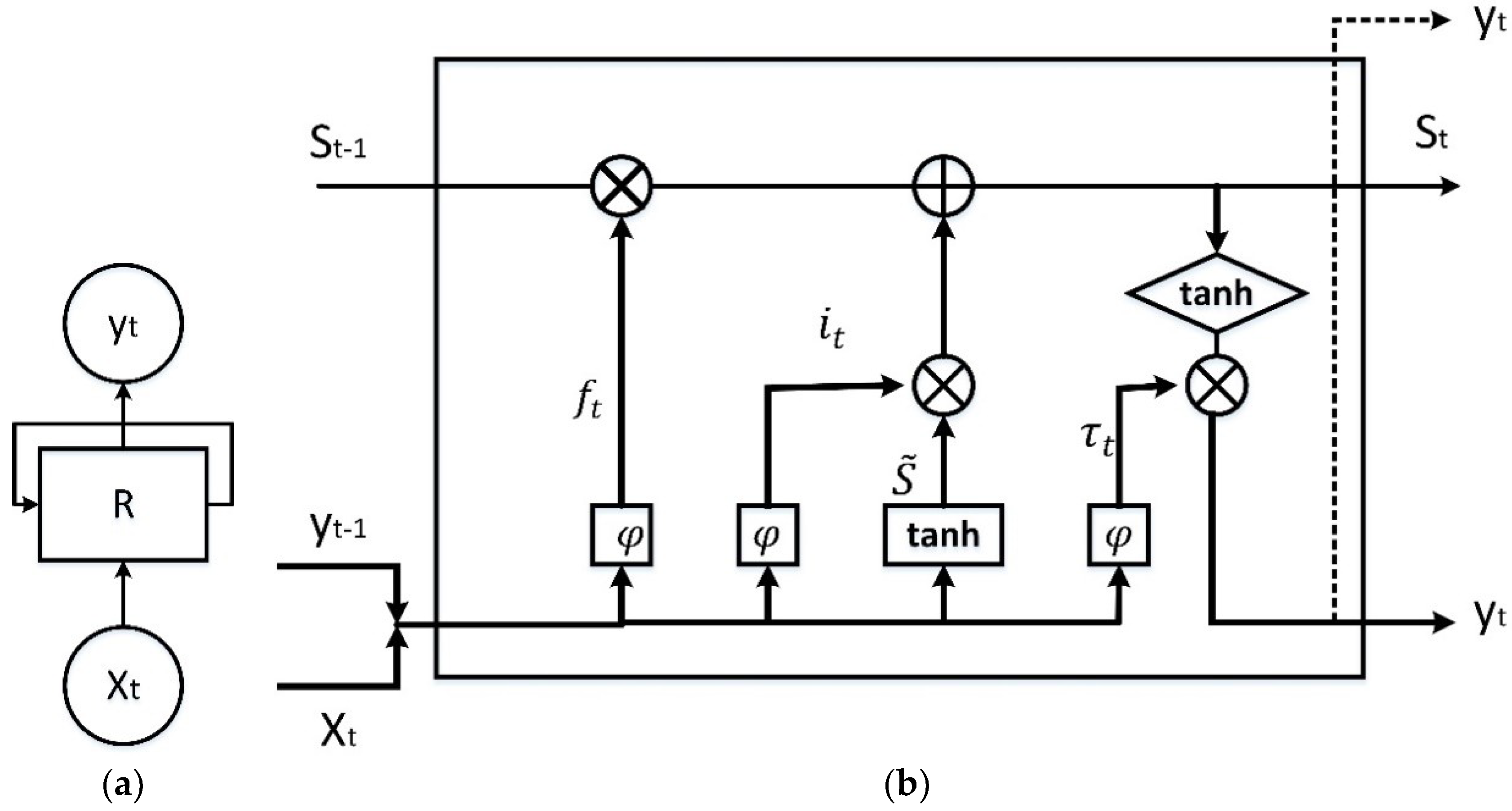
Recurrent neural network (RNN) is one of the classes of deep ANNs that is widely used in training models for time-dependent data. As shown in Figure 3a, unlike conventional multilayer perceptron, RNN uses a network of feedback loops to recall the value from the prior time step. This makes RNN a proper tool to deal with time-series applications such as character and speech recognition [32], image captioning, etc.
Although RNNs could work well in theory in recognition and prediction of long-term dependencies, in practice, several problems have been identified and reported in applying them to carry out tasks, including a long span between relevant information of input and the related output point [33,34]. For instance, RNN has challenges for accurate long-term electrical load forecasting as the machine trains with vast amounts of time series data to predict a long future period. Long short term memory (LSTM) was proposed as a solution to this issue [35]. LSTMs can recall the information for a long period of time and are broadly used in a wide range of tasks. Although the structure of the repeating modules in RNN is straightforward and typically consists of a single “” layer, LSTM modules have a more complex composition, consisting of various kinds of gates to let the information through, or be forgotten [26]. A schematic illustration of one LSTM module is provided in Figure 3b.
In long-term electrical load forecasting, sometimes, the model needs to forget about the sudden changes in power consumption because of power failure or natural disaster a long time ago. Therefore, there should be a layer in the LSTM model for forgetting the past data that is not required to be passed to the next module. The “forget layer” in the initial step is responsible for deciding what types of information could be passed on and what information should be rejected by using a binary function. Using and as inputs, and with the help of an activation function (), it generates numbers between 0 and 1 as output. Simply, 0 means forget the new information, and 1 means the information can be added to the cell state of the previous module (St-1). The output ( is calculated as
where and are weight and bias parameters, respectively, and is the output of the prior LSTM module.
The next stage consists of two steps; first, specifying the value that should be updated () and then creating a vector of new candidates’ values () through a function [24].
These values are then used to adjust the prior cell state to as below:
Eventually, the output () can be evaluated based on the calculated cell state that is specified based on a sigmoid function to find out the parts of the cell state that go to output (), and a function that generates the values between −1 and 1:
In every neural network, the weights should be optimized in each layer, over the training iterations. In the training process, we used “Adam” and “RMSprop” optimizers rather than the conventional gradient descent algorithm, which is time-consuming and resource-intensive [36].
Nonlinear autoregressive exogenous (NARX) neural network is another class of ANN that is proper for dealing with time-series data, and has shown good performance in the literature, for predicting electricity load. NARX can be mathematically expressed by the below equation [37]:
where and are output and input of the network, respectively, at time step n; and are input and output memory orders, respectively; and k represents the delay term. Based on Equation (16), the general NARX method could be evaluated by the following equation [38]:
The independent variables have different ranges of values, and to remove the dimensionality issue and make the training process faster, we employed a min-max scaler normalization:
We applied a regularization technique, called "dropout", to prevent the overfitting of the neural network. With this method, during the training process, the model randomly selects some neurons and temporarily removes their contribution to the activation and updating weights of downstream and upstream layers (in the forward pass and backpropagation, respectively). This avoids overfitting by removing overdependence on the neighbor layers throughout the network [39].
To evaluate the performance of prediction models, we considered root mean square error (RMSE), coefficient of determination (R2) and mean absolute percentage error (MAPE) to find out the goodness of the fit. RMSE is a simple technique to evaluate a model’s error:
where is the predicted value and is the actual (observed) value. The mean absolute percentage error is also calculated as below:
R2, on the other hand, is a statistical measure of how the fitted regression line is near the actual data and is determined as
where is the average of observed values. The R2 value is between zero and one, and the closer values to 1 show a better fit.
4. Results
4.1. Case Study
In this research, Bruce County, a small rural region located in the southwest of Ontario, Canada, is selected as the case study. This region has a total area of 4079 km2 and a population of 68,147 as of 2016 [40]. There are different energy sources used by power generation units in the Ontario province. Although most of the energy comes from nuclear power, other sources such as solar, wind, hydropower, and fossil fuels are also used in Ontario as a source of energy [41]. The initial dataset is created by concatenating the hourly weather data retrieved from the open-source environmental and natural resources database, provided by the government of Canada [42] and the hourly electricity consumption dataset of Bruce County, recorded from 2010 to 2019 and prepared by the Independent Electricity System Operator (IESO) which is also publicly available for download [43]. IESO is the Smart Metering Entity of Ontario, responsible for the implementation and operation of the province’s meter data. The weather dataset had several attributes; however, based on the most used features in literature [4,36,44] as well as testing the significance of their contribution to the prediction (through trial and error), the most important ones; i.e., temperature and wind speed, are selected in this case study as independent variables.
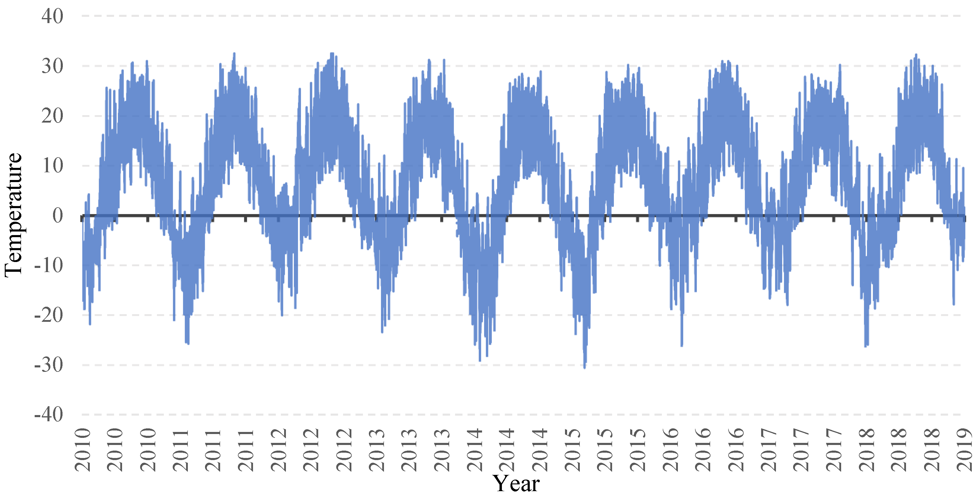
Figure 4 shows variations in the temperature for Bruce County during the entire ten years period. As seen, the temperature has a regular seasonal behavior with the maximum ranging from 28.2 °C to 32.5 °C in summer, and the minimum within the range of −20.1 °C to −30.6 °C in winter of various years. The electricity consumption behavior, especially in residential buildings, is strongly correlated with the exterior temperature. The wind also has some impact on the load demand, especially in winter, which can be due to the wind chill effect.
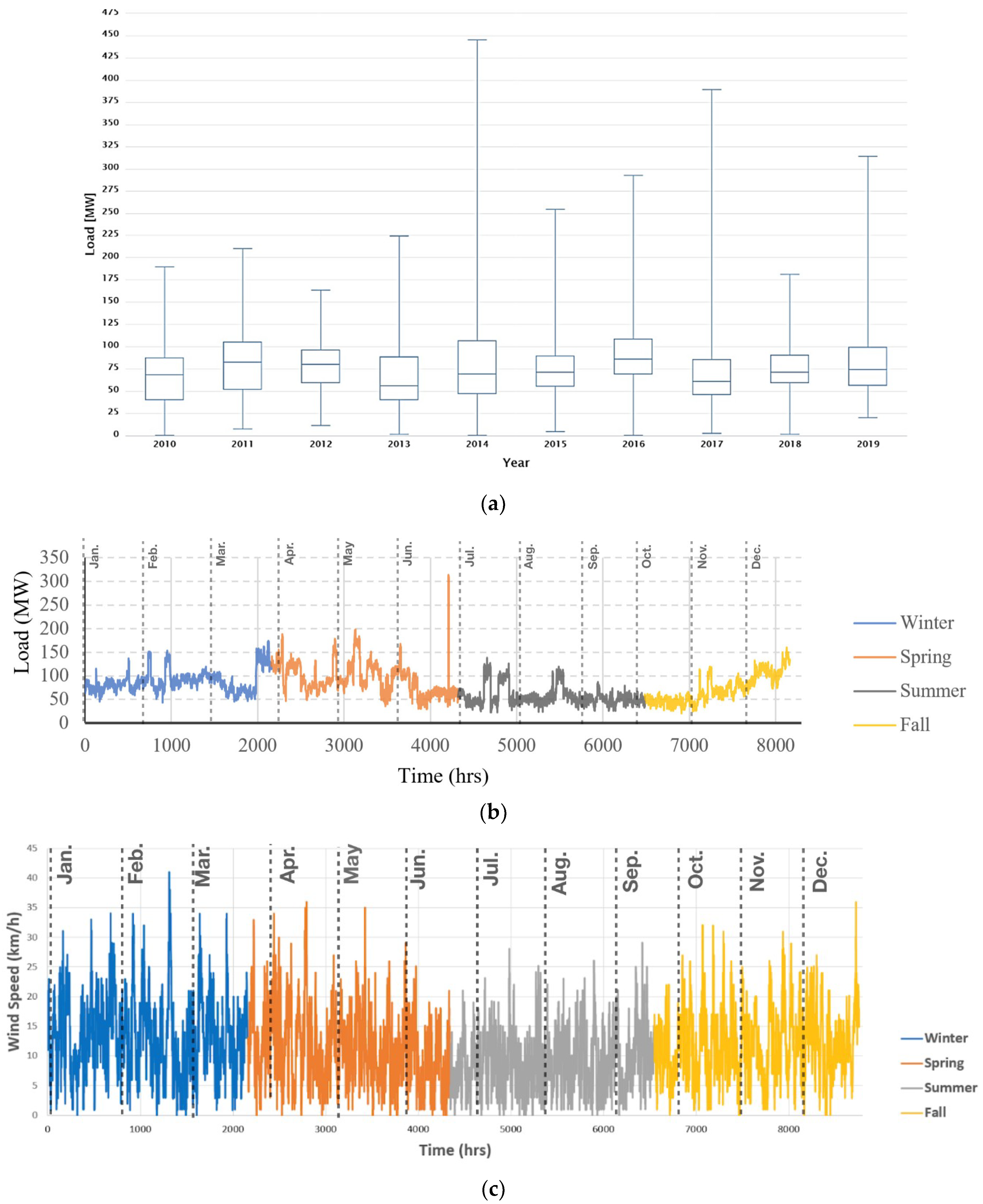
Figure 5 shows the electricity load of Bruce County. In Figure 5a, a box plot of the annual historical electrical load is presented. A peak demand with an excessively large value is observed at the end of June. As mentioned earlier, this peak is frequently repeating in other years too, around the same time. Since the aim of our prediction model is to cover such peaks, this value is not filtered out as a statistical outlier. Moreover, to better highlight the seasonality throughout a year, Figure 5b displays the hourly electricity demand in a sample year (2019, as the most recent year). As seen, the records have a broad fluctuation. It could also be observed that the electricity demand generally decreases in summers, which, given the cold climate of Bruce, can be explained by the reduction in heating demand during the months of June through August. Figure 5c,d show the hourly wind speed and temperature for the year 2019 sample, respectively. The negative correlation between temperature and electricity consumption in winter can be observed in Figure 5.
4.2. Implementation
The whole dataset consists of ten years of historical data (2010–2019). We used ten-fold validation for training our predictors; where in each fold, nine years of data were considered as training and one year as a test set. Here we explain one of the folds, i.e., using 2010–2018 as the training set and 2019 as the test set, as an example, to highlight the procedure details. For the nine other folds, similar steps were followed. For each year, the later years (and in cases, a combination of later and prior years) were used to re-create the model and then predict that years’ consumption. While this will introduce the backcasting into the predictive modeling procedure and can impose limitations to the model; given the constraints with data availability, such methods of testing have not been uncommon for working with electricity consumption time series data set [15]. The analytics of the results are presented at the end of this section. 2010–2018 as a training set has 78,840 data points and 291 missing values in electricity load, which have been replaced by the average of nearest loads preceding and succeeding them. There have been no missing values in the test set, i.e., 2019. After cleansing and preprocessing the weather and load data, we trained the three models introduced earlier. Each model was fine-tuned, and their parameters were optimized to maximize the accuracy (and minimize the error). Estimating the best values for hyperparameters of machine learning (and deep learning) models is always a challenge. As there is no closed solution to find these values, we followed a trial-and-error approach to identify optimal values for such parameters in each training task.
The RF regression entails several hyperparameters that control the model accuracy. The first is the evaluation criterion for RF. Since the data is of numerical nature, we used the least-squares method that minimizes the squared distance between the averages of values in the node with regards to the actual value. The next two are the maximum tree size and depth. The tree size was tested with different values ranging between 50 and 200, with increments of 50. The increase in the size improved the accuracy up to a certain level and then declined it. The tree size at 200 was inferior to 150; hence 150 was selected as the optimal size. The depth was tested with values of 10, 20, 25, and 30, and we did not go beyond 30 to prevent overfitting. Table 1 shows the selected optimal settings for the hyperparameters. Pre-pruning was also applied, with settings expressed in this table.
Support Vector Regression contains several hyperparameters that dictate whether the model will overfit or overgeneralize the data. Various values for misclassification tolerance, C, were used similarly to Cheng et al. [45]. Additionally, the kernel type and the number of max iterations considerably influence the computational time. After several attempts, the most optimal settings for SVR were obtained shown in Table 2. The C parameter was iterated using the values of 0, 0.01, 0.1, and 1, and the best performance, i.e., 0, was chosen. A “C” value of 0 means the strictest boundaries were set. After examining a wide range of kernel functions, we selected the dot kernel. For the other kernel types tested (i.e., radial, polynomial, neural, ANOVA, Epanechnikov, Gaussian combination, and multi-quadric), the performance was far less satisfactory (due to considerably higher values of RMSE).
Keras library with TensorFlow backend is used as an open-source neural network library to build the LSTM layers. Moreover, the GridSearchCV package from the Scikit-learn library was used to find the best hyperparameters for the LSTM, and the results are listed in Table 3. Mean squared error (MSE) was used to score each hyperparameter. The network has 20 neurons in the input layer (the size of the feature space); and one neuron in the output layer (the load forecast). The results of GridSearch show that the best optimizer is Adam, while the premier batch size and number of epochs are 32 and 10, respectively. Considering a greater number of values and types for each hyperparameter tremendously increases the optimization time and computational cost. As mentioned in the methodology section, to avert the overfitting issue, some of the neurons should be dropped out in each layer. In this study, 20 percent of the neurons were dropped out in each layer. For the NARX network, the only two parameters that required manual input were the number of hidden layers and the delay. They were set to 10 and 168, respectively.
5. Discussion
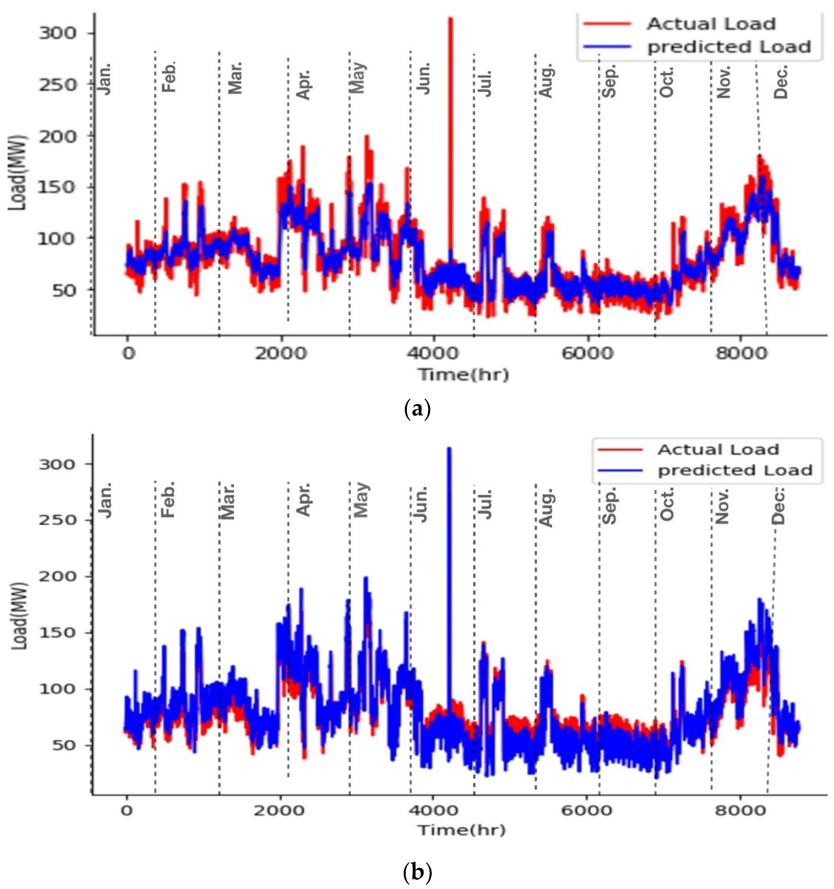
Figure 6 demonstrates the actual versus predicted loads of the three models, for 2019 as an example. As mentioned in the methodology, coefficient of determination (R2) and RMSE were used for evaluating the models’ performance. Results of the optimal RF showed an R2 of 0.871, RMSE of 11.925 MW, and MAPE of 10.25% for forecasting the electricity load of 2019 in Bruce County, both of which are within an acceptable range when compared with the literature [4]. It can be seen, however, from Figure 6a that the model consistently struggled to predict peak load demands, often underestimating the lows and overestimate the high peaks. Loads closer to the mean are associated with lower error values. Using the same training and test datasets, the optimal SVR model obtained an R2, RMSE, and MAPE of 0.877, 12.308 MW, and 14.11%, respectively (for predicting 2019). As seen in Figure 6b, while SVM was able to predict the large center peak, noticeable inaccuracies, as in RF, occur when attempting to predict peak load demands closer to the mean. The LSTM model could accurately predict even the peak load demands, with an R2 of 0.93, the RMSE of about 8.3MW, and the MAPE of 10.21%. Last but not least, the NARX neural network RMSE for forecasting a year ahead (2019) load demand is 5.81 while the R2 and MAPE are 0.96 and 4.2%, respectively.
To overcome the issue of bias in testing and evaluating the performance of all three models, a 10-fold validation was performed. Table 4 reports the average, standard deviation, and range of the evaluation metrics, achieved from the cross-validation. As seen in this table, the accuracy ranges achieved from SVM and LSTM models are very close and slightly higher than the RF models. The exact same observation can be reported on the prediction models’ errors. The NARX model, however, has a better performance in terms of the mean and standard deviation of determination coefficient and root mean square error.
As seen, it is clear that NARX has performed better than LSTM, SVM, and RF from all various viewpoints; i.e., accuracy, error, time, and pattern. While all four models could acceptably predict the overall load demand, the main difficulty was the prediction of peaks. RF’s predicted loads consistently failed to match the maxima and minima (peaks) of the load demand, while SVM failed at times to predict the minima, and at other intervals the maxima. LSTM predictions, however, had considerably better conformance with the peaks, with mismatches mainly occurring for minimum peaks. Nonetheless, the NARX model had a considerably lower mismatch, even when compared with LSTM. Given the higher sensitivity of most smart grid applications to the maxima, such a mismatch can be of a lower level of significance from an application point of view. Another critical factor was the computational time involved. Table 4 shows the training time for one fold of each model, using an Intel(R) Core i7 (7th Gen)—7500U CPU @ 2.7GHz, RAM 16 GB, platform running Windows 10 Pro 64bits. The results indicate that the RF method is involved in a much shorter training time than other methods. However, between SVM and LSTM that both showed strong prediction ability and less error than the RF; the LSTM model converges about three times faster than the SVM model. Since in practice, the models are not meant to be deployed in real-time and the training will not be repeated on a large frequency; the computation time will not be the most critical criteria for model selection. Overall, the NARX model could be selected as the proper model with the least error and acceptable computational time.
Validation with the Literature
In 2020, Jung et al. used various machine learning models to forecast regional electrical load in Seoul with a time horizon of one month [46]. They used 12 years (2005–2017) monthly electric load data of 25 districts in Seoul as a training set. In addition to weather data such as temperature and humidity, calendar and population datasets were deployed as input variables. The average MAPE of all districts for Multiple Linear Regression (MLR), RF, Extreme Gradient Boost (XGB), and DNN model were 11.90, 8.00, 6.86, and 6.46, respectively, for two years predicted (2017–2018). Although the time horizon (and accordingly the lookback period) that is in Seung-Min et al. publication is one month and considerably smaller than one year used in the present study, the results of our research (especially the LSTM and NARX neural network) are superior in terms of the accuracy of forecasting.
6. Conclusions
Growth of smart girds and moving towards decentralized and intermittent energy production, together with the emergence of prosumers who at the same time with consuming electricity can produce energy, have made the prediction of electricity demand at urban (regional/district) scale more critical as well as challenging. While digitalization offers sensing technologies that provide real-time visibility of the grid status with high refresh rates; still balancing the highly stochastic supply-demand fluctuations at a district- and region-scale remains an urgent need. As data becomes more widely available, and computational power becomes more efficient and affordable, machine learning techniques become feasible for addressing such problems. Previous efforts in this regard are proven to be effective in demand prediction for energy utility companies whose short- and long-term energy planning rely on predicting sophisticated patterns. In this paper, we focused on various techniques of machine learning, ensemble learning, and deep learning to predict electricity demand with an hourly resolution at a regional scale. RF, SVM, LSTM, and NARX neural network were four techniques considered, ranging from computationally simplistic to complex, respectively. As demonstrated in our experiment, all four models showed viability in prediction, and they can precisely forecast the trends to various degrees. The noise available in the historical data (such as negative values for electricity consumption) was handled in the preprocessing stage. Some fluctuations in demand, which statistically appear as noise, were not removed from the training data, as they were frequently repeated through various years, hence were considered to reflect the nature of the electrical consumption of the region. The LSTM model was parametrically optimized to inhibit the one-time sudden changes (due to unexpected environmental extremes or sudden power failures) in the learning process while keeping the seasonality effects. It was shown by this study that the complexity of LSTM modules, and most importantly, having different layers for forgetting and passing new information, could successfully distinguish between the two different behavior. Therefore, while the seasonal extremes could be successfully predicted by our deep learning model, the model was not distracted by the ad hoc fluctuations.
The novelty of our reported method has roots in (i) developing tuned recurrent neural network (long short-term memory) for district-level load prediction; (ii) development of the Non-linear Autoregressive Exogenous model to evaluate the impact of the recurrent dynamic network on the accuracy of predicting the unexpected behavior of the load demand; and (iii) benchmarking and cross-comparison of various tuned models based on accuracy and computational cost, to support decision making for the selection of a proper model to be fed by urban big data and make predictions at the scale of a district. The main contributions of this study include firstly, showing the feasibility of using machine learning techniques for predicting the energy demand of a municipality for the medium term on an hourly basis. Secondly, we determined the LSTM and NARX neural network as the superior algorithms compared to SVM and RF. Our results showed that RF and SVM are not the best choices when there is sensitivity on predicting peak electrical consumption, especially when the reason for load forecasting is control and energy management of an energy system. Our LSTM and NARX models, however, properly predicted the trends for both peak and off-peak values, with maximum accuracy and minimum error. The adaptability of LSTM and NARX appears to be the key in predicting the time-series of load demand for Bruce County. NARX neural network proved the most accurate prediction with R2 of 0.96 and RMSE of 5.81 MW for a window size of 168 h. This was superior to the R2 values of 0.93, 0.871, and 0.877 and RMSE values of 8.3 MW, 11.925 MW, and 12.31 MW for LSTM, RF, and SVM, respectively. While our results indicate the superiority of NARX over the machine learning tools examined; in the future, the experiment can be repeated with other publicly available datasets (such as the Global Energy Forecasting Competition) before generalizing the findings into other similar cases.
This study had some limitations too. Firstly, the windowing size (i.e., selection of the analysis period) played a significant role in computation time. The analysis window sizes above a week would take beyond one day to complete the calculations for the SVR computation. Hence, we limited the models’ resolution to computationally affordable windows. On the other hand, our models were trained on the first nine (9) years and tested on the tenth year. The effect of cross-validation in terms of shuffling the training and test years must be investigated in the future, particularly to identify the impact of long-term effects (such as climate change) on the prediction accuracy. Moreover, future studies should investigate methods to improve the accuracy of computationally simpler models (such as RF and SVM). For example, splitting the energy demand data into the peak and off-peak demand times and training separate models for these cases is virtually expected to improve the accuracy. This can be specifically helpful for the cases lacking big data, where deep learning methods may not be as effective and accurate. Studying the sensitivity of methods’ accuracy to the data size and specifications can also be among the questions for future research. Furthermore, considering larger analysis window sizes, studying the effect of window size, and finding the optimal size is another vital aspect of our future studies. Combining more comprehensive pre-processing procedures, such as grouping sub-regions with similar behavior through clustering, and using the results in training the prediction models can also help to improve the accuracy, and should be investigated in the future. There are other types of methods developed for dealing with time-series data, such as the Elman method, and authors will try to compare the results of this study with the accuracy of these methods for predicting the load demand in future research.
Author Contributions
Conceptualization, M.N.-B.; methodology, M.N.-B., and N.S.; software, N.S., A.N., and M.K.; validation, M.N.-B., N.S., A.N., and M.K.; formal analysis, N.S., A.N., and M.K.; investigation, M.N.-B., N.S., A.N., and M.K.; resources, N.S., A.N., and M.K.; data curation, N.S., A.N., and M.K.; writing—original draft preparation, N.S., A.N., and M.K.; writing—review and editing, M.N.-B.; visualization, N.S., A.N., and M.K.; supervision, M.N.-B. All authors have read and agreed to the published version of the manuscript.
Funding
This research received support from the Fonds Québecois de la Recherche sur la Nature et les Technologies (FRQNT) through ‘Établissement de nouveaux chercheurs et de nouvelles chercheuses universitaires’ program.
Informed Consent Statement
Not applicable.
Data Availability Statement
Publicly available datasets were analyzed in this study. This data can be found here: [ https://www.ieso.ca/en/Power-Data/Data-Directory (accessed on 8 December 2020)] and [https://climate.weather.gc.ca/historical_data/search_historic_data_e.html (accessed on 20 June 2020)].
Conflicts of Interest
On behalf of all authors, the corresponding author states that there is no conflict of interest.
References
- Cook, J.; Nuccitelli, D.; Green, S.A.; Richardson, M.; Winkler, B.; Painting, R.; Way, R.; Jacobs, P.; Skuce, A. Quantifying the consensus on anthropogenic global warming in the scientific literature. Environ. Res. Lett. 2013, 8. [Google Scholar] [CrossRef] [Green Version]
- Braun, M.R.; Altan, H.; Beck, S.B.M. Using regression analysis to predict the future energy consumption of a supermarket in the UK. Appl. Energy 2014, 130, 305–313. [Google Scholar] [CrossRef] [Green Version]
- Jenkins, D.; Liu, Y.; Peacock, A.D. Climatic and internal factors affecting future UK office heating and cooling energy consumptions. Energy Build. 2008, 40, 874–881. [Google Scholar] [CrossRef]
- Ahmad, T.; Chen, H. Potential of three variant machine-learning models for forecasting district level medium-term and long-term energy demand in smart grid environment. Energy 2018, 160, 1008–1020. [Google Scholar] [CrossRef]
- Soliman, S.A.; Al-kandari, A.M. Electrical Load Forecasting. Modeling and Model Construction; Butterworth-Heinemann: Oxford, UK, 2010; ISBN 0123815444. [Google Scholar]
- Karthika, S.; Margaret, V.; Balaraman, K. Hybrid short term load forecasting using ARIMA-SVM. Innov. Power Adv. Comput. Technol. i-PACT 2017, 2017, 1–7. [Google Scholar] [CrossRef]
- Li, Q.; Ren, P.; Meng, Q. Prediction Model of Annual Energy Consumption of Residential Buildings. In Proceedings of the 2010 International Conference on Advances in Energy Engineering, ICAEE, Beijing, China, 19–20 June 2010; IEEE: New York, NY, USA, 2010; pp. 223–226. [Google Scholar]
- Jain, R.K.; Smith, K.M.; Culligan, P.J.; Taylor, J.E. Forecasting energy consumption of multi-family residential buildings using support vector regression: Investigating the impact of temporal and spatial monitoring granularity on performance accuracy. Appl. Energy 2014, 123, 168–178. [Google Scholar] [CrossRef]
- Ruiz-Abellón, M.D.C.; Gabaldón, A.; Guillamón, A. Load forecasting for a campus university using ensemble methods based on regression trees. Energies 2018, 11, 2038. [Google Scholar] [CrossRef] [Green Version]
- Ahmad, M.W.; Mourshed, M.; Rezgui, Y. Trees vs Neurons: Comparison between random forest and ANN for high-resolution prediction of building energy consumption. Energy Build. 2017, 147, 77–89. [Google Scholar] [CrossRef]
- Wang, Z.; Wang, Y.; Zeng, R.; Srinivasan, R.S.; Ahrentzen, S. Random Forest based hourly building energy prediction. Energy Build. 2018, 171, 11–25. [Google Scholar] [CrossRef]
- Khan, P.W.; Byun, Y.C.; Lee, S.J.; Kang, D.H.; Kang, J.Y.; Park, H.S. Machine learning-based approach to predict energy consumption of renewable and nonrenewable power sources. Energies 2020, 13, 4870. [Google Scholar] [CrossRef]
- Khan, P.W.; Byun, Y.-C. Genetic Algorithm Based Optimized Feature Engineering and Hybrid Machine Learning for Effective Energy Consumption Prediction. IEEE Access 2020, 8, 196274–196286. [Google Scholar] [CrossRef]
- Khan, P.W.; Byun, Y.C.; Lee, S.J.; Park, N. Machine learning based hybrid system for imputation and efficient energy demand forecasting. Energies 2020, 13, 2681. [Google Scholar] [CrossRef]
- Lahouar, A.; Ben Hadj Slama, J. Day-ahead load forecast using random forest and expert input selection. Energy Convers. Manag. 2015, 103, 1040–1051. [Google Scholar] [CrossRef]
- Neto, A.H.; Fiorelli, F.A.S. Comparison between detailed model simulation and artificial neural network for forecasting building energy consumption. Energy Build. 2008, 40, 2169–2176. [Google Scholar] [CrossRef]
- Biswas, M.A.R.; Robinson, M.D.; Fumo, N. Prediction of residential building energy consumption: A neural network approach. Energy 2016, 117, 84–92. [Google Scholar] [CrossRef]
- Hong, T.; Pinson, P.; Fan, S. Global energy forecasting competition 2012. Int. J. Forecast. 2014, 30, 357–363. [Google Scholar] [CrossRef]
- Bendaoud, N.M.M.; Farah, N. Using deep learning for short-term load forecasting. Neural Comput. Appl. 2020, 32, 15029–15041. [Google Scholar] [CrossRef]
- Thokala, N.K.; Bapna, A.; Chandra, M.G. A deployable electrical load forecasting solution for commercial buildings. In Proceedings of the 2018 IEEE International Conference on Industrial Technology (ICIT), Lyon, France, 20–22 February 2018; Volume 2018, pp. 1101–1106. [Google Scholar] [CrossRef]
- Koschwitz, D.; Frisch, J.; van Treeck, C. Data-driven heating and cooling load predictions for non-residential buildings based on support vector machine regression and NARX Recurrent Neural Network: A comparative study on district scale. Energy 2018, 165, 134–142. [Google Scholar] [CrossRef]
- Agrawal, R.K.; Muchahary, F.; Tripathi, M.M. Long term load forecasting with hourly predictions based on long-short-term-memory networks. In Proceedings of the 2018 IEEE Texas Power and Energy Conference (TPEC), College Station, TX, USA, 8–9 February 2018; Volume 2018, pp. 1–6. [Google Scholar] [CrossRef]
- Lee, S.; Cho, S.; Kim, S.-H.; Kim, J.; Chae, S.; Jeong, H.; Kim, T. Deep Neural Network Approach for Prediction of Heating Energy Consumption in Old Houses. Energies 2020, 14, 122. [Google Scholar] [CrossRef]
- Shi, H.; Xu, M.; Li, R. Deep Learning for Household Load Forecasting-A Novel Pooling Deep RNN. IEEE Trans. Smart Grid 2018, 9, 5271–5280. [Google Scholar] [CrossRef]
- Tarik Rashid, B.Q.; Huang, M.-T.K.; Gleeson, B. Auto-Regressive Recurrent Neural Network Approach for Electricity Load Forecasting. Int. J. Comput. Intell. 2006, 3, 1304–2386. Available online: https://www.researchgate.net/publication/287828870_Auto-regressive_recurrent_neural_network_approach_for_electricity_load_forecasting (accessed on 20 June 2020).
- Rahman, A.; Srikumar, V.; Smith, A.D. Predicting electricity consumption for commercial and residential buildings using deep recurrent neural networks. Appl. Energy 2018, 212, 372–385. [Google Scholar] [CrossRef]
- Warrior, K.P.; Shrenik, M.; Soni, N. Short-Term Electrical Load Forecasting Using Predictive Machine Learning Models. In Proceedings of the 2016 IEEE Annual India Conference, INDICON, Bangalore, India, 16–18 December 2016. [Google Scholar]
- Li, C.; Tao, Y.; Ao, W.; Yang, S.; Bai, Y. Improving forecasting accuracy of daily enterprise electricity consumption using a random forest based on ensemble empirical mode decomposition. Energy 2018, 165, 1220–1227. [Google Scholar] [CrossRef]
- Grolinger, K.; L’Heureux, A.; Capretz, M.A.M.; Seewald, L. Energy forecasting for event venues: Big data and prediction accuracy. Energy Build. 2016, 112, 222–233. [Google Scholar] [CrossRef] [Green Version]
- Du, K.L.; Swamy, M.N.S. Neural Networks in a Softcomputing Framework; Springer-Verlag: London, UK, 2006; ISBN 1846283027. [Google Scholar]
- Goodfellow, I.; Bengio, Y.; Courville, A. Deep Learning; MIT Press: Cambridge, MA, USA, 2016; Available online: http://www.deeplearningbook.org (accessed on 20 December 2020).
- Zhang, X.Y.; Yin, F.; Zhang, Y.M.; Liu, C.L.; Bengio, Y. Drawing and Recognizing Chinese Characters with Recurrent Neural Network. IEEE Trans. Pattern Anal. Mach. Intell. 2018, 40, 849–862. [Google Scholar] [CrossRef] [Green Version]
- Hochreiter, S. Untersuchungen zu Dynamischen Neuronalen Netzen. Diploma Thesis, Technische Universität München, München, Germany, 1991. [Google Scholar]
- Bengio, Y.; Simard, P.; Frasconi, P. Patrice Simard; Paolo Frasconi Learning Long-term Dependencies with Gradient Descent is Difficult. IEEE Trans. Neural Netw. 1994, 5, 157. [Google Scholar] [CrossRef]
- Hochreiter, S.; Schmidhuber, J. Long Short-Term Memory. Neural Comput. 1997, 9, 1735–1780. [Google Scholar] [CrossRef]
- Wen, L.; Zhou, K.; Yang, S.; Lu, X. Optimal load dispatch of community microgrid with deep learning based solar power and load forecasting. Energy 2019, 171, 1053–1065. [Google Scholar] [CrossRef]
- Menezes, J.M.P.; Barreto, G.A. Long-term time series prediction with the NARX network: An empirical evaluation. Neurocomputing 2008, 71, 3335–3343. [Google Scholar] [CrossRef]
- Ardalani-Farsa, M.; Zolfaghari, S. Chaotic time series prediction with residual analysis method using hybrid Elman-NARX neural networks. Neurocomputing 2010, 73, 2540–2553. [Google Scholar] [CrossRef]
- Srivastava, N.; Hinton, G.; Krizhevsky, A.; Sutskever, I.; Salakhutdinov, R. Dropout: A Simple Way to Prevent Neural Networks from Overfitting. J. Mach. Learn. Res. 2014, 15, 1929–1958. [Google Scholar]
- Census Profile, 2016 Census—Bruce, County [Census Division], Ontario and Newfoundland and Labrador [Province], (n.d.). Available online: https://www12.statcan.gc.ca/census-recensement/2016/dp-pd/prof/details/page.cfm?Lang=E&Geo1=CD&Code1=3541&Geo2=PR&Code2=10&Data=Count&SearchText=Bruce&SearchType=Begins&SearchPR=01&B1=All&TABID=1 (accessed on 10 August 2020).
- Data Directory, (n.d.). Available online: http://www.ieso.ca/en/ (accessed on 28 April 2020).
- Historical Data—Climate—Environment and Climate Change Canada, (n.d.). Available online: https://climate.weather.gc.ca/historical_data/search_historic_data_e.html (accessed on 20 June 2020).
- Data Directory, (n.d.). Available online: https://www.ieso.ca/en/Power-Data/Data-Directory (accessed on 8 December 2020).
- Gurubel, K.J.; Osuna-Enciso, V.; Cardenas, J.J.; Coronado-Mendoza, A.; Perez-Cisneros, M.A.; Sanchez, E.N. Neural forecasting and optimal sizing for hybrid renewable energy systems with grid-connected storage system. J. Renew. Sustain. Energy 2016, 8. [Google Scholar] [CrossRef]
- Cheng, Y.; Xu, C.; Mashima, D.; Thing, V.L.L.; Wu, Y. PowerLSTM: Power Demand Forecasting Using Long Short-Term Memory Neural Network. In Proceedings of the Advanced Data Mining and Applications: 13th International Conference, Singapore, 5–6 November 2017; Springer: Berlin/Heidelberg, Germany, 2017. Available online: https://0-link-springer-com.brum.beds.ac.uk/chapter/10.1007/978-3-319-69179-4_51 (accessed on 5 April 2020).
- Jung, S.M.; Park, S.; Jung, S.W.; Hwang, E. Monthly electric load forecasting using transfer learning for smart cities. Sustainability 2020, 12, 6364. [Google Scholar] [CrossRef]
Figure 1.
High-level methodology of this study.
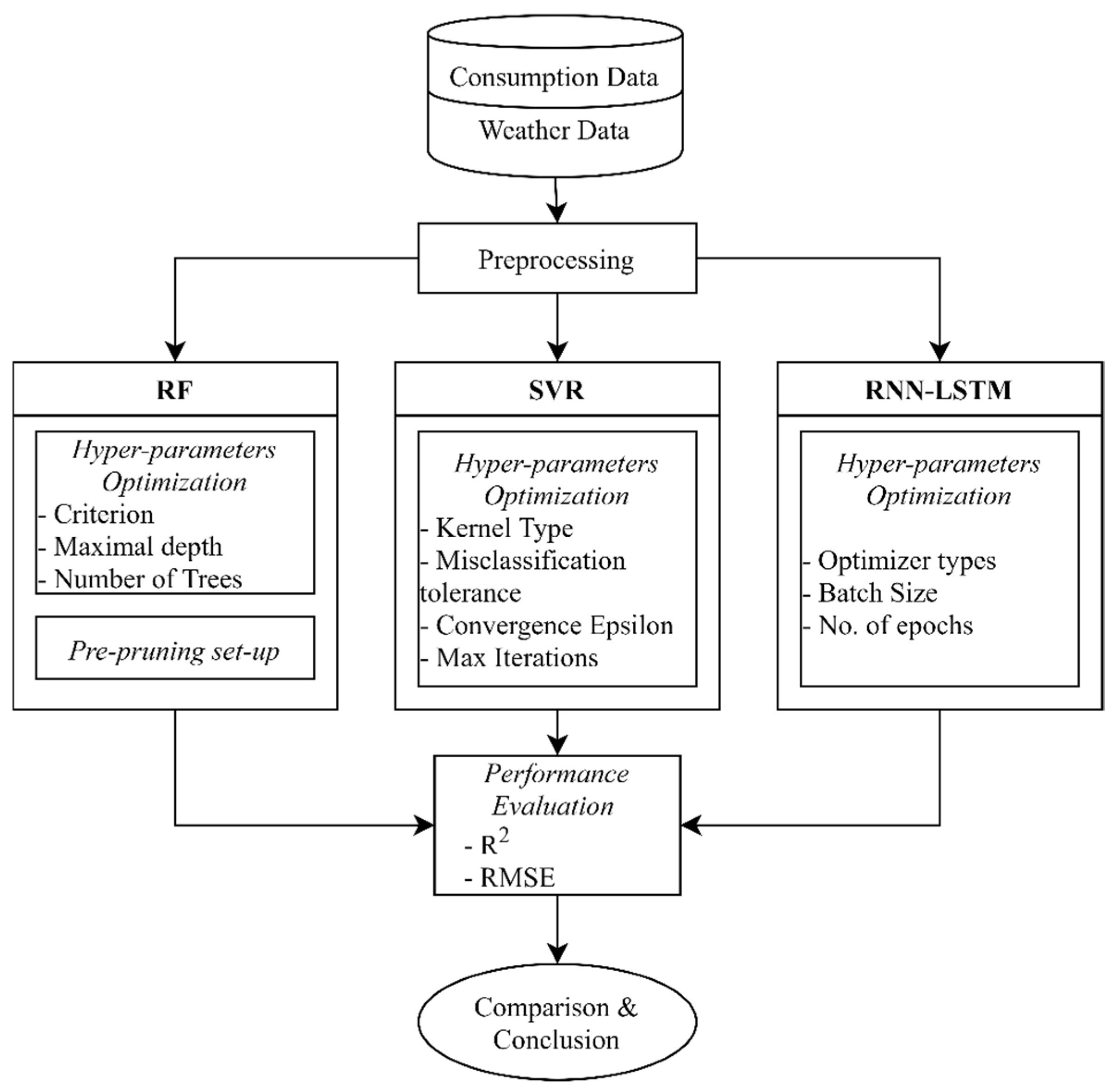
Figure 2.
Visualization of Support Vector Regression (SVR) parameters (regenerated based on [29]).
Figure 2.
Visualization of Support Vector Regression (SVR) parameters (regenerated based on [29]).
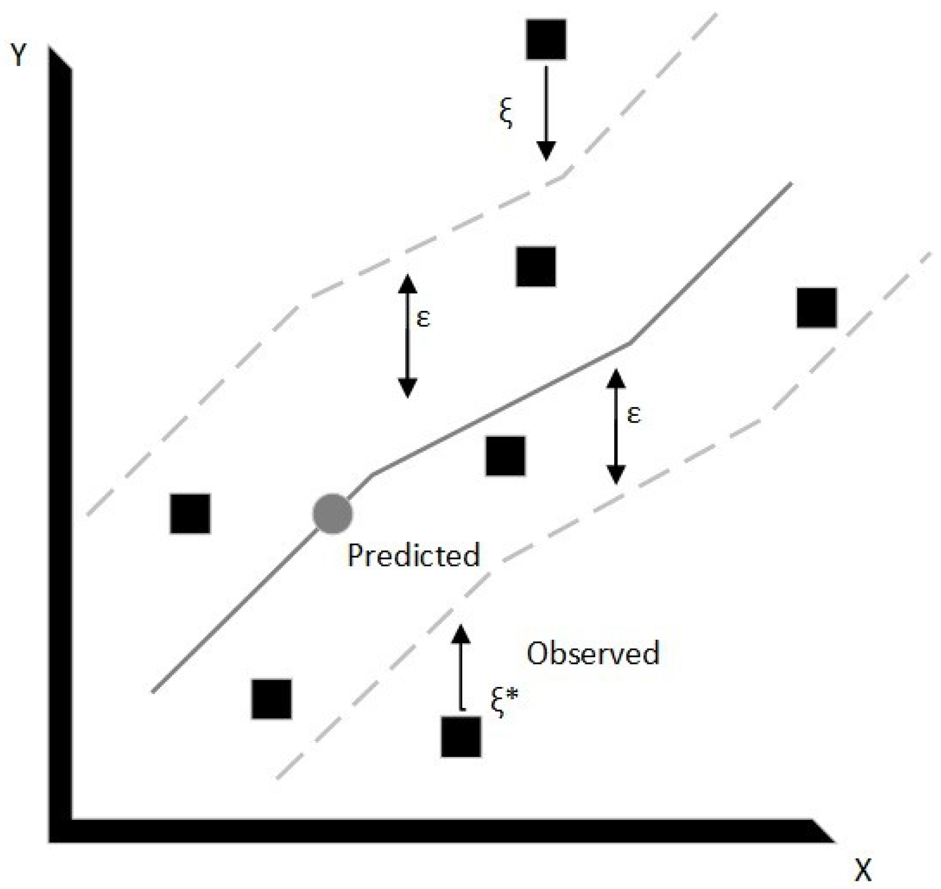
Figure 3.
Schematic view of the recurrent neural networks (RNN) model—Long Short-Term Memory (LSTM) Method. (a) RNN loop; (b) inside of the LSTM module (regenerated from [24]).
Figure 3.
Schematic view of the recurrent neural networks (RNN) model—Long Short-Term Memory (LSTM) Method. (a) RNN loop; (b) inside of the LSTM module (regenerated from [24]).

Figure 4.
Temperature trend in training set data.

Figure 5.
(a) Electrical consumption load trend in 10 years (from 2010 until the end of 2019); (b) Hourly electrical consumption load in a sample year (2019); (c) Hourly wind speed in a sample year (2019); (d) Hourly Temperature in a sample year (2019).
Figure 5.
(a) Electrical consumption load trend in 10 years (from 2010 until the end of 2019); (b) Hourly electrical consumption load in a sample year (2019); (c) Hourly wind speed in a sample year (2019); (d) Hourly Temperature in a sample year (2019).

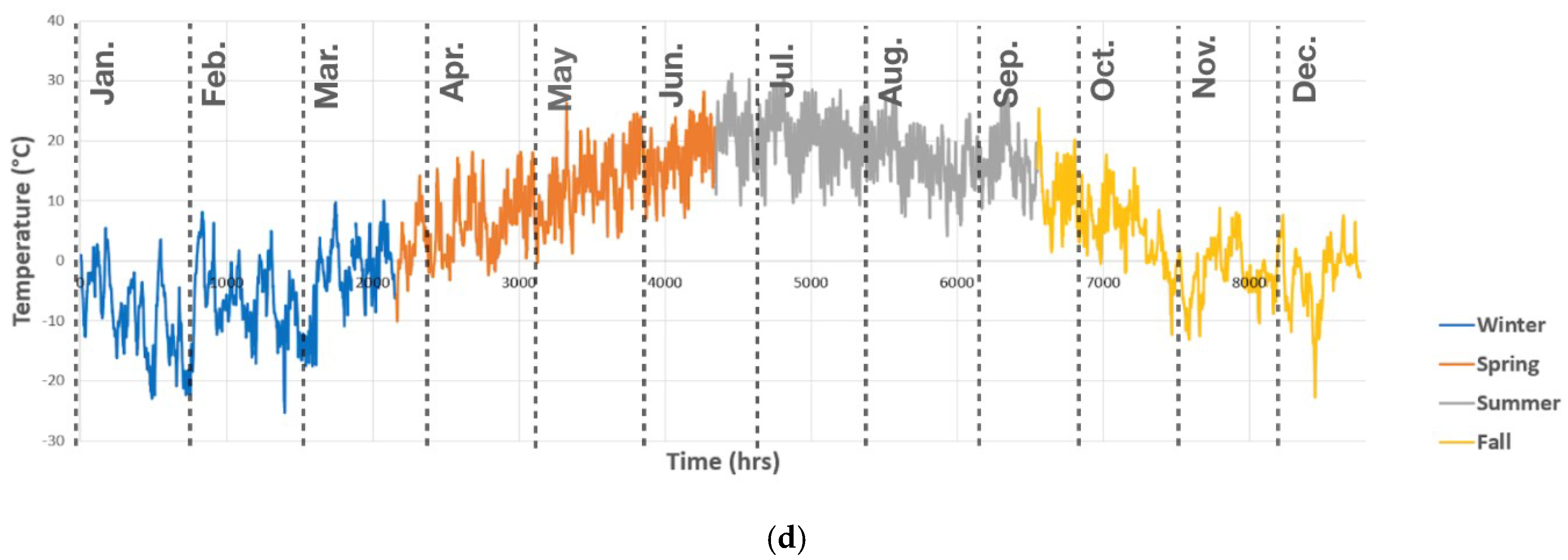
Figure 6.
Comparison of prediction models, forecasted load vs. observed data (for 2019). (a) RF regression model; (b) SVR model; (c) LSTM model; (d) Non-linear auto-regressive exogenous (NARX) model.
Figure 6.
Comparison of prediction models, forecasted load vs. observed data (for 2019). (a) RF regression model; (b) SVR model; (c) LSTM model; (d) Non-linear auto-regressive exogenous (NARX) model.


Table 1.
Hyperparameters of Random Forest (RF) model that considered for optimization.
| Parameters | Setting | |
|---|---|---|
| Criterion | Least Squares | |
| Maximal depth | 30 | |
| Number of Trees | 150 | |
| Pre-pruning parameters | Minimal gain | 0.01 |
| Minimal leaf size | 2 | |
| Minimal size for split | 4 | |
| Number of pre-pruning alternatives | 3 |
Table 2.
Hyperparameters of the Support Vector Machine (SVM) model that considered for optimization.
Table 2.
Hyperparameters of the Support Vector Machine (SVM) model that considered for optimization.
| Parameters | Setting |
|---|---|
| Kernel Type | dot |
| Misclassification tolerance, C | 0 |
| Convergence Epsilon, ε | 0.001 |
| Max Iterations | 10,000 |
Table 3.
Hyperparameters of LSTM model that considered for optimization.
| Parameters | Values/Types |
|---|---|
| No. hidden layers | 3 |
| No. neurons per hidden layer | 50 |
| Activation function | Hyperbolic tangent (tanh) |
| Optimizer types | {Adam, RMSprop} |
| Batch Size | {20,25,32} |
| No. of epochs | {5,10,15,20} |
Table 4.
Statistics of the evaluation metrics (accuracy and error) for each model based on 10-fold cross-validation.
Table 4.
Statistics of the evaluation metrics (accuracy and error) for each model based on 10-fold cross-validation.
| Model | RMSE | R2 | Computation Time (min) | ||
|---|---|---|---|---|---|
| Mean ± SD | Range | Mean ± SD | Range | ||
| LSTM | 9.569 ± 3.050 | [7.16,15.00] | 0.921 ± 0.0341 | [0.85,0.95] | 93 |
| NARX | 6.987 ± 1.433 | [5.52,9.75] | 0.953 ± 0.0142 | [0.93,0.98] | 16 |
| SVM | 11.878 ± 2.447 | [7.89,15.22] | 0.886 ± 0.0345 | [0.84,0.94] | 244 |
| RF | 13.028 ± 3.483 | [10.05,21.49] | 0.853 ± 0.0489 | [0.78,0.91] | 50 |
Publisher’s Note: MDPI stays neutral with regard to jurisdictional claims in published maps and institutional affiliations. |
© 2021 by the authors. Licensee MDPI, Basel, Switzerland. This article is an open access article distributed under the terms and conditions of the Creative Commons Attribution (CC BY) license (https://creativecommons.org/licenses/by/4.0/).
Share and Cite
MDPI and ACS Style
Shirzadi, N.; Nizami, A.; Khazen, M.; Nik-Bakht, M. Medium-Term Regional Electricity Load Forecasting through Machine Learning and Deep Learning. Designs 2021, 5, 27. https://0-doi-org.brum.beds.ac.uk/10.3390/designs5020027
AMA Style
Shirzadi N, Nizami A, Khazen M, Nik-Bakht M. Medium-Term Regional Electricity Load Forecasting through Machine Learning and Deep Learning. Designs. 2021; 5(2):27. https://0-doi-org.brum.beds.ac.uk/10.3390/designs5020027
Chicago/Turabian StyleShirzadi, Navid, Ameer Nizami, Mohammadali Khazen, and Mazdak Nik-Bakht. 2021. "Medium-Term Regional Electricity Load Forecasting through Machine Learning and Deep Learning" Designs 5, no. 2: 27. https://0-doi-org.brum.beds.ac.uk/10.3390/designs5020027