An Improved Extended Kalman Filter for Radar Tracking of Satellite Trajectories

Abstract

Nonlinear state estimation problem is an important and complex topic, especially for real-time applications with a highly nonlinear environment. This scenario concerns most aerospace applications, including satellite trajectories, whose high standards demand methods with matching performances. A very well-known framework to deal with state estimation is the Kalman Filters algorithms, whose success in engineering applications is mostly due to the Extended Kalman Filter (EKF). Despite its popularity, the EKF presents several limitations, such as exhibiting poor convergence, erratic behaviors or even inadequate linearization when applied to highly nonlinear systems. To address those limitations, this paper suggests an improved Extended Kalman Filter (iEKF), where a new Jacobian matrix expansion point is recommended and a Frobenius norm of the cross-covariance matrix is suggested as a correction factor for the a priori estimates. The core idea is to maintain the EKF structure and simplicity but improve its accuracy. In this paper, two case studies are presented to endorse the proposed iEKF. In both case studies, the classic EKF and iEKF are implemented, and the obtained results are compared to show the performance improvement of the state estimation by the iEKF.

1. Introduction

Nonlinear state estimation is a desirable and required tool in several engineering applications, especially in aerospace, where it is crucial for tasks such as surveillance, guidance, navigation, attitude control, obstacle avoidance and target tracking [1,2,3,4,5,6]. The problem consists of estimating the state vector (which contains all relevant information to describe the system of the moving target) based on noisy measurements, imperfect models, inaccurate data acquisition systems and environmental perturbations that are unwanted and, in most cases, also unknown [7]. Wrong estimates can lead to wrong information about the states and, consequently, wrong control feedback. Therefore, the development of methods that can provide reliable state estimates is extremely important.

The concern for optimal filtering methods began in the early 1940s, with Wiener and Kolmogorov [8,9]. They solved the estimation problem for stochastic processes based on the linear least square. Wiener developed the solution for continuous-time, and Kolmogorov developed the solution for discrete-time. Nowadays, this filter is known as the Wiener filter and is still important; however, it is restricted to stationary signals only. In 1960, Rudolf Kalman continued Wiener’s research for a more generic nonstationary process, resulting in the Kalman Filter (KF) [10]. The main difference between these two filters is that the Wiener filter was developed in the frequency domain and is mainly used for signal estimation, whereas the Kalman Filter was developed in the time domain and is mainly used for state estimation.

The KF has a form of feedback control, which means, first, the filter estimates the process state at a specific time and then obtains feedback in the form of noisy measurements. It can be defined as an optimal online recursive data-processing algorithm.

In the past decades, the KFs were the most widely used tool to deal with nonlinear state estimation, mostly because of the Extended Kalman Filter (EKF), which was initially developed for the Apollo Mission [11,12]. The EKF is based on the assumption that a local linearization of the system may be a sufficient description of nonlinearities; therefore, the linearized model is used instead of the original nonlinear function [13,14,15,16]. Such approximations are extremely easy to apply, which explains the popularity of the filter. However, when dealing with highly nonlinear systems, the EKF estimates suffer serious problems, such as unstable and quickly divergent behaviors, poor linearization and/or erratic behaviors [17,18,19,20].

Afterwards, a large number of strategies and variations were developed [2,21,22,23,24,25,26,27,28,29,30,31], for example, the unscented, cubature, ensemble Kalman Filters, infinity norm filter or even the particle filter. The key problem with these nonlinear filtering methods is to balance the computational complexity with the desired estimation accuracy. Most of those methods require intensive calculations, which also means more computational time, and consequently a significant limitation for crucial time applications. Some methods (e.g., infinity norm filter) require more tuning to get acceptable performance, and this is not ideal for nonlinear systems performing in time-critical environments. This is one of the reasons why this filter is not as popular as the Kalman Filter. Another reason is, while in Kalman Filtering, different approaches lead to the same (or similar) equations, with the infinity norm filtering, different approaches lead to widely different equations [31].

Acknowledging that EKF is one of the most popular algorithms to deal with radar tracking and to address its limitations, this paper proposes an improved Extended Kalman Filter (iEKF) with an adaptive structure. A new a priori covariance matrix calculation is proposed, as well as a new Jacobian expansion point. For the covariance matrix, we suggest a Frobenius norm of the cross-covariance matrix as a correction factor for the a priori estimate. Regarding the Jacobian expansion point, we suggest an average between the linearization point and the filtered state to obtain a point closer to the true state. By choosing a more adequate point and a more reliable covariance, it is possible to ensure better stability and precision. The initial results were presented in Reference [32], where the proposed method was validated in a ballistic missile radar tracking problem. In this current manuscript, the techniques are updated, and new case studies are analyzed. In this paper, the iEKF is validated on a satellite orbit estimation and a Hohmann Transfer, where the position and velocity of the satellite are estimated. The root mean square estimation error (RMSE) was used to compare straightforwardly both filters, EKF and iEKF. The iEKF RMSE is considerably smaller than the EKF RMSE, which suggests that the iEKF algorithm copes better with nonlinear systems when compared to the classic EKF.

This paper is organized as follows: In the next section, the problem statement is briefly summarized. The EKF and the iEKF are described in the subsequent sections. Section 4 presents the simulations and results, where the filters’ performances are compared and evaluated. This is followed by conclusions and future work in Section 5.

2. Problem Statement

The main objective of the nonlinear state estimation problem in the context of radar tracking is to accurately estimate the state of a moving target based on a sequence of noisy measurements.

This paper adopts a state-space approach with discrete-time formulation, simply because it is more convenient for real-time applications, such as radar tracking [33,34].

A general stochastic state-space representation of a nonlinear time-discrete model has the following form:

$$x_k=f\left(x_{k-1},u_{k-1}\right)+w_{k-1}$$

(1)

$$y_k=h\left(x_k\right)+v_k$$

(2)

where Equation (1) is responsible for describing the evolution of the system states with time; Equation (2) is responsible for relating the state of the system with the measurements; $x_k\in {ℝ}^n$ represents the state vector at the time-step $k$, which can be defined as a set of variables that provide the complete status of the system at that time; $y_k\in {ℝ}^m$ is the measurement vector at the time-step $k$; $f\left(.\right)$ is a general nonlinear function of the dynamic model; $h\left(.\right)$ is a general function of the measurement model; $u_k\in {ℝ}^r$ is the control inputs vector; and $w_k$ and $v_k$ are white zero-mean uncorrelated process and measurement noise, whose covariance matrix $Q_k$ and $R_k$ are given, respectively, by the following:

$$w_k\sim N\left(0,Q_k\right) \mathrm{with} E\left[w_k{w}_j^T\right]=Q_k{\delta }_k$$

(3)

$$v_k\sim N\left(0,R_k\right) \mathrm{with} E\left[v_k{v}_j^T\right]=R_k{\delta }_k$$

(4)

$$E\left[v_k{w}_j^T\right]=0$$

(5)

where ${\delta }_k$ is the Kronecker delta function: if $k=j$, then ${\delta }_k=1$; if $k\ne j$, then ${\delta }_k=0$ [34]; $E$ is the statistical moment of a variable.

The functions $f\left(.\right)$ and $h\left(.\right)$ from Equations (1) and (2) depend on the time-step $k$, but for notational convenience, this dependence is not explicitly denoted.

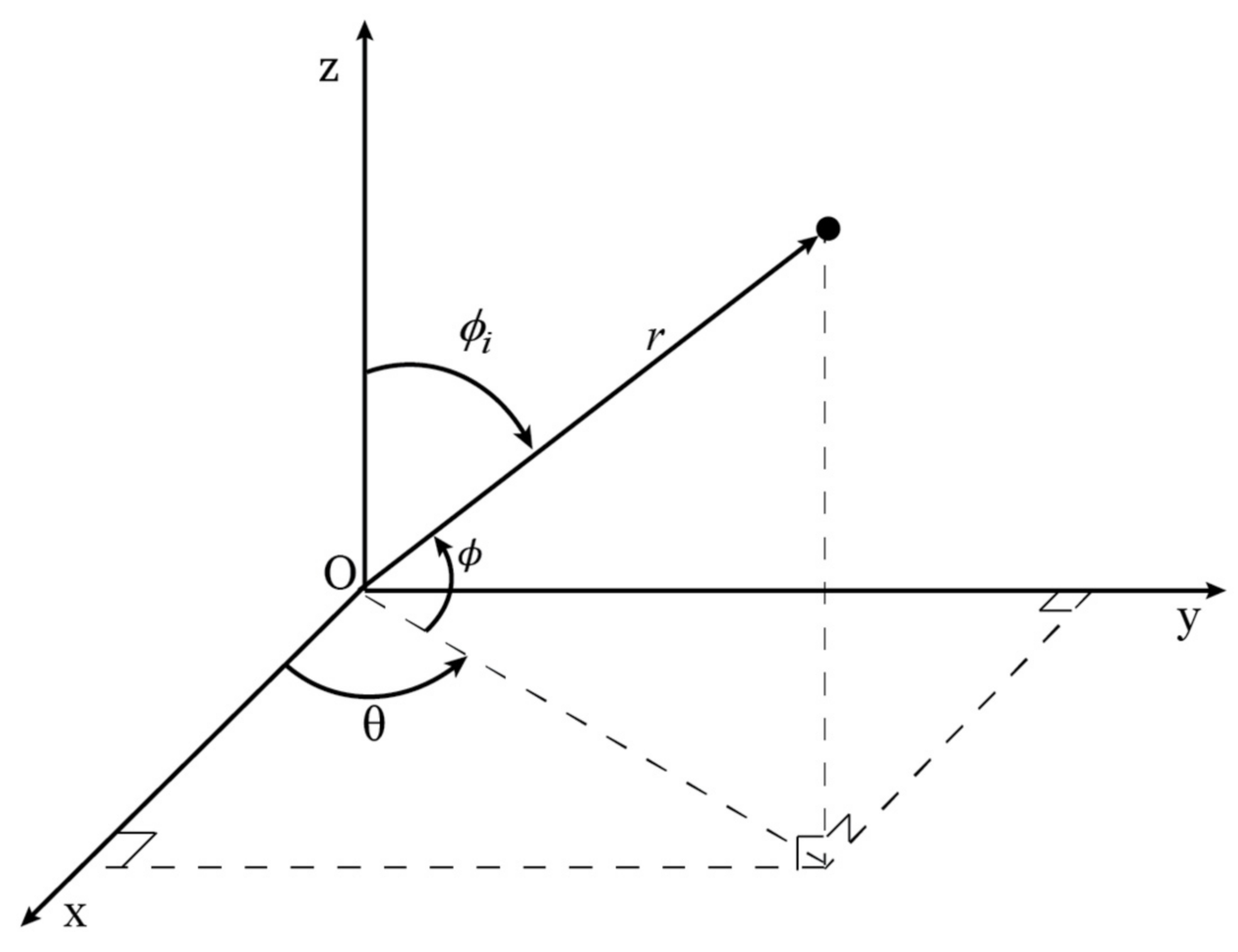
The study cases presented in this paper assume that the radar has a fixed position, and the sensor provides the following measurements: target range ($r$), azimuth angle ($\theta$) and elevation angle ($\varphi$), as shown in Figure 1. Regarding these coordinates, $r$ represents the radial distance between the radar and the aerospace vehicle (target), $\theta$ represents the angle measured from X-axis in XY plane of an inertial rectangular coordinate system to the projection of $r$ onto XY plane and, lastly, $\varphi$ represents the angle measured from the projection of $r$ onto XY plane to the vector $r$.

Therefore, Equation (2) can be expressed in the following form:

$$y_k=\left(\begin{array}{c}{r}_k+v_{1,k}\\ {\theta }_k+v_{2,k}\\ {\varphi }_k+v_{3,k}\end{array}\right)=\left(\begin{array}{c}\sqrt{x_k^2+y_k^2+z_k^2}+v_{1,k}\\ {\tan }^{-1}\left(\frac{y_k}{x_k}\right)+v_{2,k}\\ {\sin }^{-1}\left(\frac{z_k}{r_k}\right)+v_{3,k}\end{array}\right)$$

(6)

where $v_{1,k}$, $v_{2,k}$ and $v_{3,k}$ represent the white Gaussian noise of each coordinate $\left(r,\theta ,\varphi \right)$ respectively, on the time-step $k$. The coordinates $\left(x,y,z\right)$ represent the target position on the X-axis, Y-axis, and Z-axis respectively, which form the state vector, and they are given by the following:

$$x_k=r_k\cos {\theta }_k\cos {\varphi }_k$$

(7)

$$y_k=r_k\sin {\theta }_k\cos {\varphi }_k$$

(8)

$$z_k=r_k\sin {\varphi }_k$$

(9)

The derivatives of Equations (7)–(9) are defined by the following:

$$\frac{d{x}_k}{dt}=\cos \left({\theta }_k\right)\cos \left({\varphi }_k\right)-r_k\sin \left({\theta }_k\right)\cos \left({\varphi }_k\right)-r_k\cos \left({\theta }_k\right)\sin \left({\varphi }_k\right)$$

(10)

$$\frac{d{y}_k}{dt}=\sin \left({\theta }_k\right)\cos \left({\varphi }_k\right)+r_k\cos \left({\theta }_k\right)\cos \left({\varphi }_k\right)-r_k\sin \left({\theta }_k\right)\sin \left({\varphi }_k\right)$$

(11)

$$\frac{d{z}_k}{dt}=\sin \left({\varphi }_k\right)+r_k\cos \left({\varphi }_k\right)$$

(12)

3. Nonlinear Kalman Filters

Most of the real-world systems are inherently nonlinear, and this is one of the greatest challenges in controllers’ and observers’ designs. A majority of solutions are only approximate solutions that try to cope with the existence of nonlinearities, namely the nonlinear Kalman Filters.

The KF solution can diverge due to one or more of the following reasons [3,35]:

• Modeling errors because the algorithm assumes models that are only an approximation.
• Incorrect a priori statistics, for example, the a priori covariance matrix.
• Incorrect initial conditions.
• Disturbances that are so large that the linearization becomes inadequate to describe the system accurately enough.
• Errors in computation.

3.1. Extended Kalman Filter

The EKF is a recursive process with the ability to linearize the nonlinear model by using first-order Taylor series expansion, meaning that it has the ability to linearize around the current mean and covariance.

The EKF is based on the assumption that a local linearization of the system may be a sufficient description of the nonlinearity. Thus, the linearized model is used instead of the original nonlinear functions [2,3,7,14].

The aforementioned transformation is given by the following:

$${\mathbf{x}}_k={\tilde{x}}_k+A_k\left(x_{k-1}-{\hat{x}}_{k-1}\right)+w_{k-1}$$

(13)

$$y_k\approx {\tilde{y}}_k+H_k\left(x_k-{\tilde{x}}_k\right)+v_k$$

(14)

where $x_k,y_k$ are, respectively, the actual state and measurement vectors; and ${\tilde{x}}_k,{\tilde{y}}_k$ are the approximate state and measurement vectors, as given by the following:

$${\tilde{x}}_k=f\left({\hat{x}}_{k-1},u_k,0\right)$$

(15)

$${\tilde{y}}_k=h\left({\tilde{x}}_k,0\right)$$

(16)

where ${\hat{x}}_k$ is the a posteriori estimate of the state at the step $k$, and it is obtained by the measurement update equation (Equation (22)); and $A_k$ is the Jacobian matrix of partial derivatives of $f\left(\cdot \right)$ with respect to $x$, and it is defined as follows:

$$A_k={\left.\frac{\partial f\left(x,u\right)}{\partial x}\right|}_{\begin{array}{l}x={\hat{x}}_{k-1}\\ u=u_{k-1}\end{array}}$$

(17)

where $H_k$ is the Jacobian matrix of partial derivatives of $h\left(\cdot \right)$ with respect to $x$, and it is defined by the following:

$$H_k={\left.\frac{\partial h\left(x\right)}{\partial x}\right|}_{x={\tilde{x}}_k}$$

(18)

It is worth mentioning that linearization is a very sensitive and important step, first because it is very susceptible to errors, and second because it allows the filter to get the best benefit from all the available a priori information.

The EKF algorithm can be presented as follows:

• Initialization:

It is assumed that ${\hat{x}}_0=x_0$ and ${\mathrm{P}}_0={\mathrm{P}}_{initial}$.

• Time update equations—Prediction Step:

The prediction of the state vector, ${\hat{x}}_k^{-}$, is given by the following:

$${\hat{x}}_k^{-}=f\left({\hat{x}}_{k-1},u_{k-1}\right)$$

(19)

The a priori covariance matrix, $P_k^{-}$, is computed as follows:

$$P_k^{-}=A_k{P}_{k-1}{A}_k^T+Q_{k-1}$$

(20)

• Measurement update equations—Correction Step:

The filter gain, $K_k$, is computed as follows:

$$K_k=P_k^{-}{H}_k^T{\left(H_k^T{P}_k^{-}{H}_k^T+R_k\right)}^{-1}$$

(21)

The state estimation, ${\hat{x}}_k$, is calculated by the following:

$${\hat{x}}_k={\hat{x}}_k^{-}+K_k\left(y_k-h\left({\hat{x}}_k^{-},0\right)\right)$$

(22)

The a posteriori covariance, $P_k$, is given by the following:

$$P_k=\left(I-K_k{H}_k\right)P_k^{-}$$

(23)

Exploiting the assumption that all transformations are quasi-linear, we see that the EKF simply linearizes all nonlinear transformations and substitutes the Jacobian matrices for the linear transformations. It is important to mention that the choice of reasonably good initial assumptions is essential for the EKF convergence.

3.2. Improved Extended Kalman Filter

It is very well-known that an ill-conditioned covariance matrix computation or an inadequate linearization point is enough to hinder the filter operation or indeed cause a divergent behavior. To address those limitations, we propose a new Jacobian matrix expansion point and a new a priori covariance matrix computation. The core idea is to maintain the EKF structure and simplicity but improve the overall performance with simple yet effective concepts.

3.2.1. Jacobian Matrix Expansion Point

The Jacobian matrices are a very sensitive and error-prone process with a significant impact on the overall filter performance. In fact, a well-chosen point will allow the filter to cope better with real-world requirements. In contrast, an unsuited Jacobian matrix calculation point may result in an ill-conditioned performance, resulting in the instability and divergence of the filter.

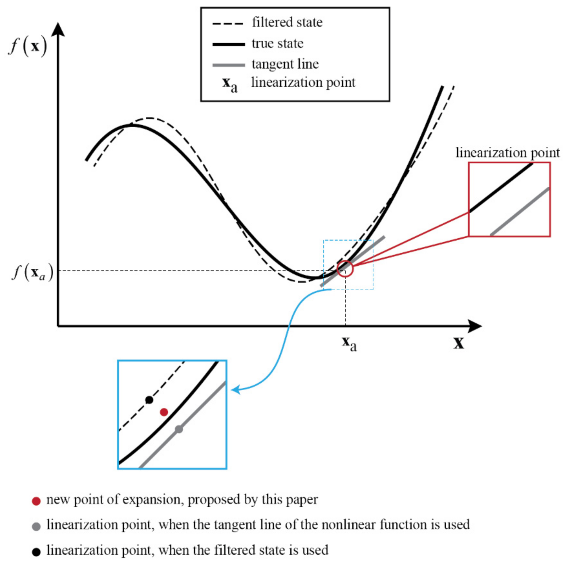
According to the mathematical analysis theory, the ith-order Jacobian matrix aims to transform ith-order errors of a nonlinear variable space to linearized function space. In this procedure, the Jacobian matrix is calculated regarding the expansion point. However, in applications with large disturbance, this point is inadequate to describe the system accurately (Figure 2). The EKF uses the filtered state as an expansion point to obtain the Jacobian matrices, but the same issue arises, especially when facing highly nonlinear environments, where estimates may be inaccurate. Consequently, it may lead to high-order truncation error and less precision on the results. Thus, the solution proposed in this paper is to use the point between the linearization point and the filtered state to obtain a point closer to the true state, as represented in Figure 2. This solution enhances the filter precision over time.

The main objective is to obtain the point that is closest to the true state, represented by the full black line in Figure 2. Therefore, the Jacobian matrices defined with the new expansion point are given by the following:

$$A_k={\left.\frac{\partial f\left(x,u\right)}{\partial x}\right|}_{\begin{array}{l}x=\frac{\left({\hat{x}}_{k-1}+x_{k-1}^{linear}\right)}{2}\\ u=u_{{}_{k-1}}\end{array}}$$

(24)

$$H_k={\left.\frac{\partial h\left(x\right)}{\partial x}\right|}_{x=\frac{\left({\tilde{x}}_k+h\left({\tilde{x}}_k,0\right)\right)}{2}}$$

(25)

where ${\hat{x}}_{k-1}$ is the a posteriori state vector given by the measurement update equation (Equation (33)), and $x_k^{linear}$ is given by $x_k^{linear}={\tilde{x}}_k+A_k\left(x_{k-1}-{\hat{x}}_{k-1}\right)+w_{k-1}$.

3.2.2. A Priori Covariance Matrix

Regarding the a priori covariance matrix, this is another significant aspect, because an ill-conditioned matrix can cause numerical instability, particularly during online implementation. It plays a crucial role in achieving good and fast convergence of the state estimates. The concern with this matrix shall start with $P_0$, because a very inadequate start can lead to a wrong end.

The covariance matrix reflects the confidence in the results; this means that, if it is very low, the filter will rely mostly on the estimates. On the other hand, if it is very high, the filter will rely mostly on the measurements.

This paper proposes the Frobenius norm of the cross-covariance matrix as a correction factor for the a priori estimate. The norm of a matrix has the ability to quantify the existing system errors and perturbations; in this case, it will behave as a correction factor:

$$P_{k-1}^{-}=\frac{P_{k-1}}{{‖P_{xy}‖}_F}$$

(26)

where ${‖.‖}_F$ represents the Frobenius norm, and $P_{xy}$ represents the cross-covariance between the state vector and the measurement vector, as given by the following:

$$P_{xy}=E\left[e_{xx}{e}_{yy}^T\right]$$

(27)

with

$$e_{xx}=\left[x_{k-1}-{\hat{x}}_k^{-}\right]$$

(28)

$$e_{yy}=\left[y_k-h\left({\hat{x}}_k^{-}\right)\right]$$

(29)

where $e_{xx}$ and $e_{yy}$ are the residuals of the dynamic and measurement models, respectively.

If the state and measurement vector have the same dimension, then it will occur a perfect matrix normalization. If not, it will occur an extension of the normalization without affecting the results.

3.2.3. Improved Extended Kalman Filter Algorithm

The iEKF algorithm can be presented as follows:

• Initialization:

It is assumed that ${\hat{x}}_0=x_0$ and ${\mathrm{P}}_0={\mathrm{P}}_{initial}$.

• Time update equations—Prediction Step:

The prediction of the state vector, ${\hat{x}}_k^{-}$, is given by the following:

$${\hat{x}}_k^{-}=f\left({\hat{x}}_{k-1},u_{k-1}\right)$$

(30)

The a priori covariance matrix, $P_k^{-}$, is computed as follows:

$$P_k^{-}=P_{k-1}{\left(P_{xy}\right)}^{-1}$$

(31)

• Measurement update equations—Correction Step:

The filter gain, $K_k$, is computed as follows:

$$K_k=P_k^{-}{H}_k^T{\left(H_k^T{P}_k^{-}{H}_k^T+R_k\right)}^{-1}$$

(32)

The state estimation, ${\hat{x}}_k$, is calculated by the following:

$${\hat{x}}_k={\hat{x}}_k^{-}+K_k\left(y_k-h\left({\hat{x}}_k^{-},0\right)\right)$$

(33)

The a posteriori (estimated) covariance, $P_k$, is given by the following:

$$P_k=\left(I-K_k{H}_k\right)P_k^{-}$$

(34)

It is important to note that, even though the measurement update equations have the same expressions as the EKF, those results will not be equal, because the Jacobian matrix point is different, so the values of $A_k$ and $H_k$ will differ, and this has a direct impact on all measurement update equations. The same happens for the a priori covariance matrix that will directly influence the Kalman gain, and the update of the covariance matrix given by Equations (32) and (33), respectively.

4. Simulations and Discussions

The main objective of this section is to apply the proposed iEKF techniques to real-time aerospace systems problems, namely the estimation of satellite orbits and orbits transferences.

In both cases, it is assumed a ground-based radar that provides range, azimuth and elevation observations of the artificial satellite. The radar is positioned in the following coordinates:

$$la{t}_{radar}=38.7755°$$

(35)

$$lon{g}_{radar}=-9.1353°$$

(36)

$$h_{radar}=45 \mathrm{m}$$

(37)

where $la{t}_{radar}$ represents the radar latitude, $lon{g}_{radar}$ represents its longitude and $h_{radar}$ represents its height.

In the next sections, the EKF and iEKF are both implemented, and the results are compared.

4.1. Case 1: Satellite Orbit Estimation

State estimation of an artificial satellite requires measurements that provide information about the satellite’s position and velocity. This paper considers discrete measurements, given by Equation (6).

The equations of motion for a satellite in the Earth’s gravitational field can be expressed in spherical coordinates [36] as follows:

$$\ddot{r}=r{\dot{\theta }}^2{\sin }^2{\varphi }_i+r{\dot{\varphi }}_i^2-\frac{{\mu }_{Earth}}{r^2}+\frac{3}{2}{\mu }_{Earth}\cdot J_2\cdot r_{Earth}\cdot \frac{3{\cos }^2\varphi -1}{r^4}+u_r$$

(38)

$$\ddot{\theta }=\frac{-2\dot{r}\dot{\theta }}{r}-2\dot{\theta }{\dot{\varphi }}_i\cot {\varphi }_i+\frac{u_{\theta }}{r\sin {\varphi }_i}$$

(39)

$${\ddot{\varphi }}_i=\frac{-2\dot{r}{\dot{\varphi }}_i}{r}+{\dot{\theta }}^2\sin {\varphi }_i\cos {\varphi }_i+3{\mu }_{Earth}\cdot J_2\cdot \frac{r_{Earth}^2}{r^5}\cdot \cos {\varphi }_i\sin {\varphi }_i+\frac{u_{\varphi }}{r}$$

(40)

where ${\mu }_{Earth}$ represents the Earth’s gravitational parameter; $r$ represents the radial distance of the space vehicle from the center of the Earth; $\theta$ represents the angle measured from the X-axis in the XY-plane of an inertial rectangular coordinate system to the projection of $r$ onto the XY-plane; ${\varphi }_i$ represents the angle between the Z-axis and the vector $r$ as represented in Figure 3; $u_r,u_{\theta },u_{\varphi }$ represent the thrust acceleration components in the ${\stackrel{⌢}{i}}_r,{\stackrel{⌢}{i}}_{\theta },{\stackrel{⌢}{i}}_{\varphi }$ directions, respectively; $r_{Earth}$ represents the Earth’s radius; and $J_2$ the second zonal harmonic.

The universal parameters are given by the following:

$$r_{Earth}=6378\times {10}^3 \mathrm{m}$$

(41)

$$G_{Earth}=6.67\times {10}^{-11}{ \mathrm{Nm}}^2{/\mathrm{kg}}^2$$

(42)

$$M_{Earth}=5.97\times {10}^{24} \mathrm{kg}$$

(43)

$${\mu }_{Earth}=G_{Earth}·M_{Earth}$$

(44)

$$J_2=1.0826\times {10}^{-3}$$

(45)

with $M_{Earth}$ representing the Earth’s mass, and $G_{Earth}$ its gravitational constant.

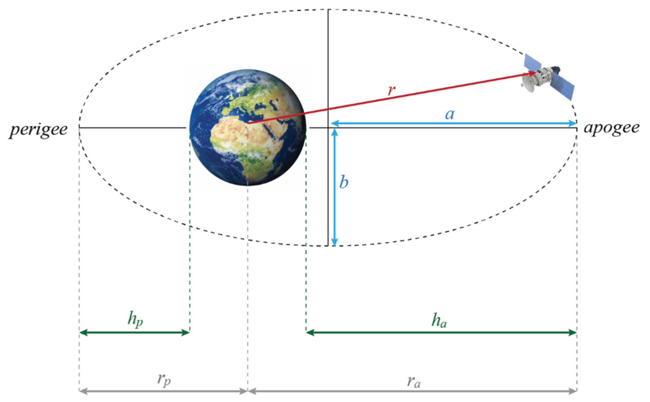
The satellite orbit follows an elliptical trajectory, as shown in Figure 4.

In Figure 4, $h_p$ represents the distance between the Earth surface and the perigee, $h_a$ represents the distance between the Earth surface and the apogee, $r_p$ represents the distance between the center of the Earth and the perigee, $r_a$ represents the distance between the center of the Earth and the apogee, $a$ represents the semi major-axis of the orbit and $b$ represents the semi minor-axis of the same orbit.

The orbital elements considered for this case are represented in

Table 1. Orbital elements for case 1: satellite orbit.

Parameter	Symbol	Value
Perigee Height	$h_p$	$200 \mathrm{km}$
Apogee Height	$h_a$	$400 \mathrm{km}$
Perigee Radius	$r_p$	$6578 \mathrm{km}$
Apogee Radius	$r_a$	$6778 \mathrm{km}$
Semi Major-Axis	$a$	$6678 \mathrm{km}$
Orbit Eccentricity	$e$	$0.01497$
Orbit Inclination	$i$	$10° \mathrm{deg}$
Orbit Period	$T$	$5433.74693 \mathrm{s}\approx 90.56 \min$

.

The Equations (38)–(40) are used to simulate the reference orbit that eventually will be tracked by the radar. The orbit is generated with the 4th-order Runge–Kutta (RK4) algorithm [37,38,39,40] (in Python), and it is initialized with the following:

$$\begin{array}{c}\left[\begin{array}{cccccc}r& \dot{r}& \theta & \dot{\theta }& \varphi & \dot{\varphi }\end{array}\right]=\\ \left[\begin{array}{cccccc}6.5780e+06& -1.2976e-01& 1.1563e-03& 1.1563e-03& 1.3963e+00& 0.0000e+00\end{array}\right]\end{array}$$

(46)

The results are represented in Figure 5.

The radar measurements of this orbit are given by Equation (6), and the error standard deviations were considered to be as follows:

$$\begin{array}{ccc}{\sigma }_r=3.16228& {\sigma }_{\theta }=1.41421& {\sigma }_{\varphi }=1.41421\end{array}$$

(47)

$$\begin{array}{cc}{\sigma }_w=9.48683& {\sigma }_v=9.48683\end{array}$$

(48)

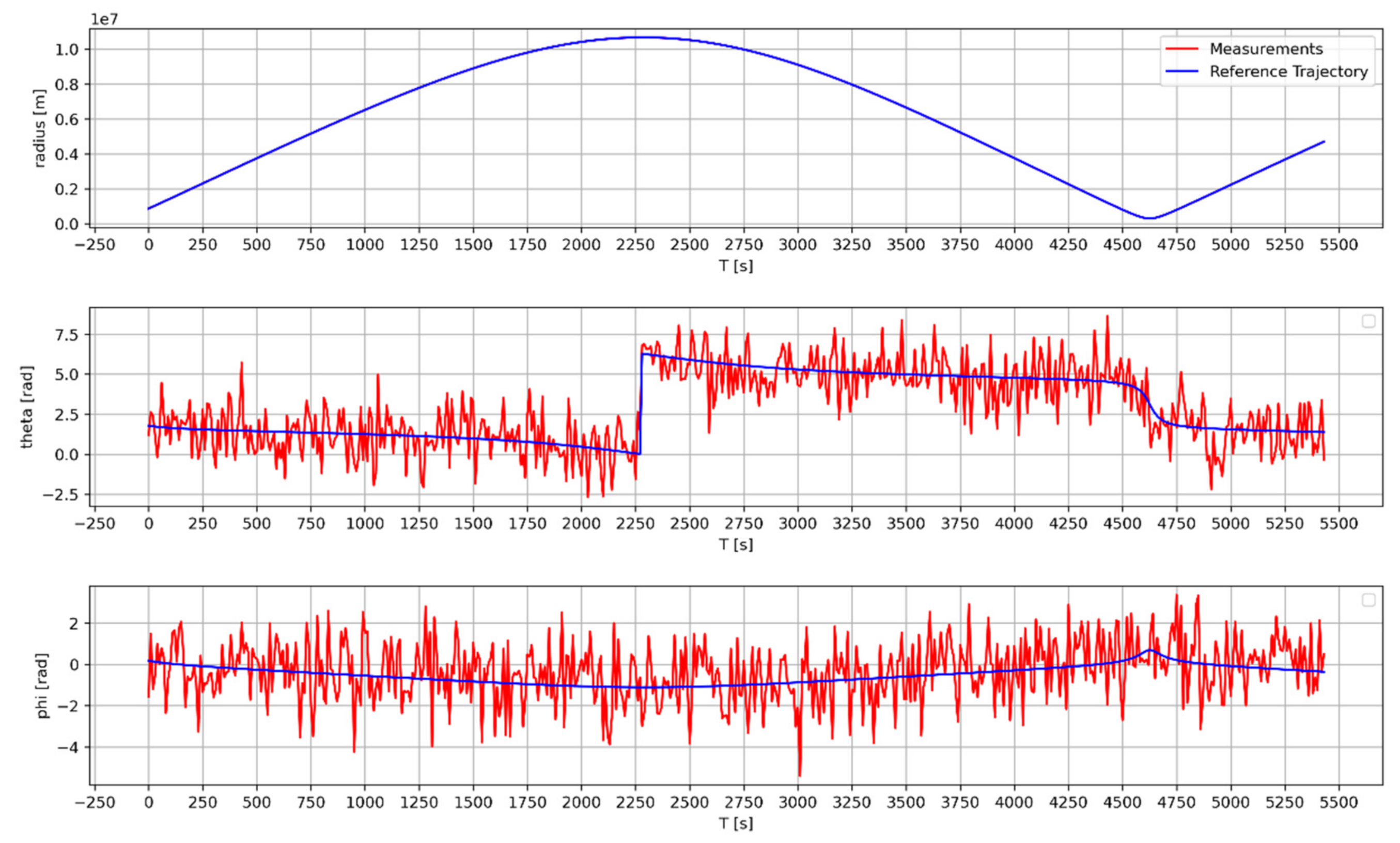
The measurement results are represented in Figure 6. The measurement $r$ coordinate (Figure 6) has noise as measurement $\theta$ and $\varphi$ coordinate, but since the range of this coordinate is very large, the difference between the reference and measurement is not visible in the figure.

The state vector is composed of the satellite Cartesian coordinates, so it is given by the following:

$$x_k=\left[\begin{array}{ccc}{x}_k& y_k& z_k\end{array}\right]$$

(49)

To initialize both filters, EKF and iEKF, we assumed the following initial conditions for ${\hat{x}}_0=\left[\begin{array}{ccc}{x}_0& y_0& z_0\end{array}\right]$ and $P_0$:

$${\hat{x}}_0=\left[\begin{array}{ccc}5279547.34311& 6106.35685& 3923823.98409\end{array}\right]$$

(50)

$$P_0=\left[\begin{array}{ccc}10.99037& 10.99037& 10.99037\\ 10.99037& 10.99037& 10.99037\\ 10.99037& 10.99037& 10.99037\end{array}\right]$$

(51)

It is noteworthy that, as occurs with the previous parameters, the values considered for the state ${\hat{x}}_0$ and $P_0$ have a high impact on the quality of the results. Therefore, it is important to make the best assumption possible.

The Jacobian matrices were calculated by the following:

$$A_k=\left[\begin{array}{ccc}\frac{\partial r_k}{\partial x}& \frac{\partial r_k}{\partial y}& \frac{\partial r_k}{\partial z}\\ \frac{\partial {\theta }_k}{\partial x}& \frac{\partial {\theta }_k}{\partial y}& \frac{\partial {\theta }_k}{\partial z}\\ \frac{\partial {\varphi }_k}{\partial x}& \frac{\partial {\varphi }_k}{\partial y}& \frac{\partial {\varphi }_k}{\partial z}\end{array}\right] \mathrm{and} H_k=\left[\begin{array}{ccc}\frac{\partial x_k}{\partial r}& \frac{\partial x_k}{\partial \theta }& \frac{\partial x_k}{\partial \varphi }\\ \frac{\partial y_k}{\partial r}& \frac{\partial y_k}{\partial \theta }& \frac{\partial y_k}{\partial \varphi }\\ \frac{\partial z_k}{\partial r}& \frac{\partial z_k}{\partial \theta }& \frac{\partial z_k}{\partial \varphi }\end{array}\right]$$

(52)

where the target range ($r_k$), the azimuth angle (${\theta }_k$) and the elevation angle (${\varphi }_k$) are given by Equation (6), as represented in Figure 1. The coordinates $x,y,z$ are given by Equations (7)–(9), respectively.

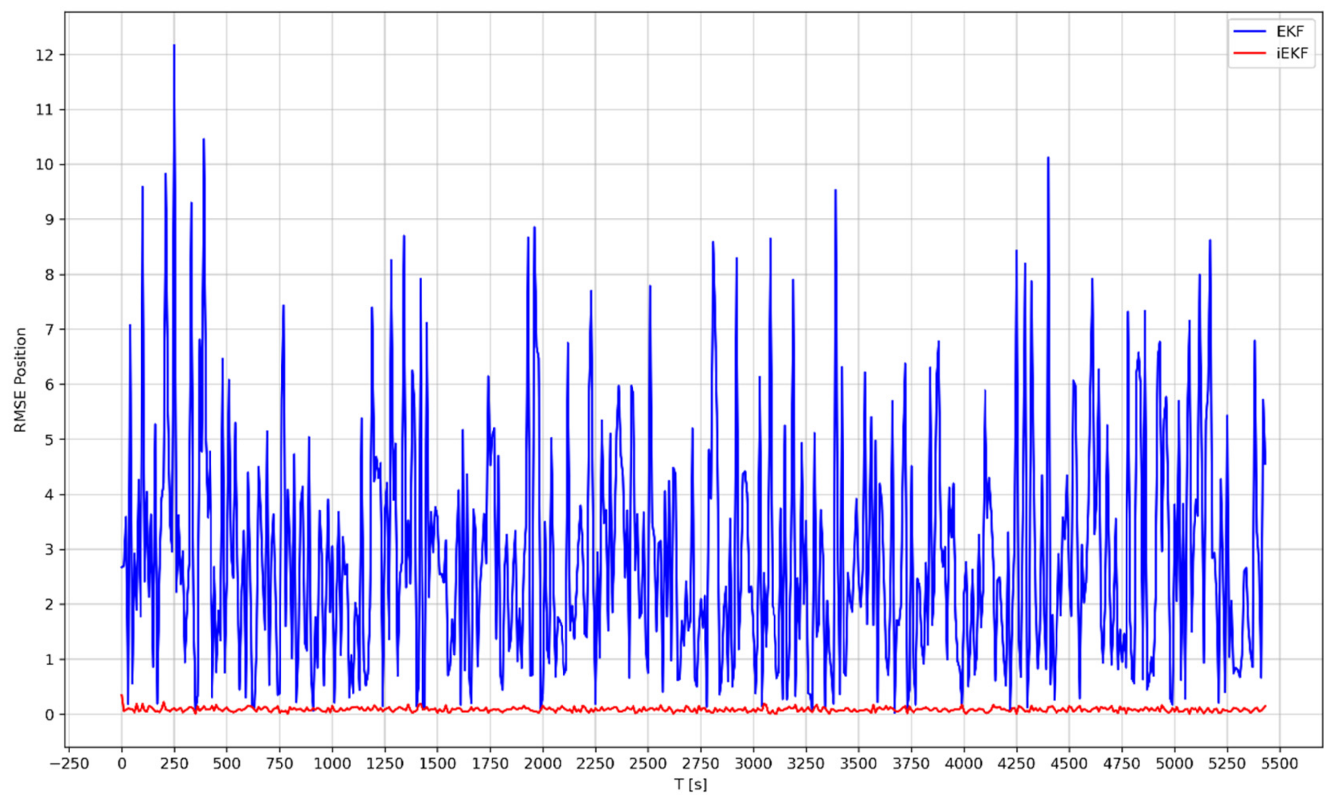
To compare the performance of each filter straightforwardly, we used the performance index RMSE (for the position and velocity), which is defined as the root mean square estimation error and is given by the following:

$$RMS{E}_{position}={\left(\frac{{\displaystyle \sum _{k=1}^{T_s}\left[{\left(x_k-{\hat{x}}_k\right)}^2+{\left(y_k-{\hat{y}}_k\right)}^2+{\left(z_k-{\hat{z}}_k\right)}^2\right]}}{T_s}\right)}^{\raisebox{1ex}{$1$}\!\left/ \!\raisebox{-1ex}{$2$}\right.}$$

(53)

$$RMS{E}_{velocity}={\left(\frac{{\displaystyle \sum _{k=1}^{T_s}\left[{\left(v_k-{\hat{v}}_k\right)}^2\right]}}{T_s}\right)}^{\raisebox{1ex}{$1$}\!\left/ \!\raisebox{-1ex}{$2$}\right.}$$

(54)

where $T_s$ is the total time steps used during the simulation, $v_k$ is the reference velocity, $v_k=\sqrt{{\dot{x}}_k^2+{\dot{y}}_k^2+{\dot{z}}_k^2}$; and ${\hat{v}}_k$ is the estimated velocity, ${\hat{v}}_k=\sqrt{{\hat{\dot{x}}}_k^2+{\hat{\dot{y}}}_k^2+{\hat{\dot{z}}}_k^2}$.

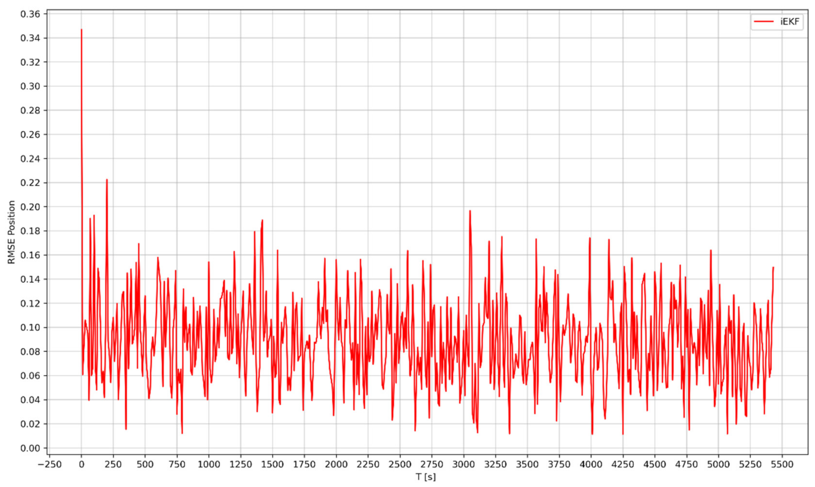
Figure 7, Figure 8, Figure 9 and Figure 10 illustrate a comparison between the EKF RMSE (blue line) and iEKF RMSE (red line) for the position and velocity. It is observable that by changing the Jacobian matrix point and the a priori covariance matrix, it is possible to obtain more accurate results. The new iEKF presents an error of less than 0.22 m for the position except the first point while the EKF presents an error of less than 12 m, which is quite a significant difference. The first spike of Figure 8 is the initialization point. It is higher than the others, which indicate that the (assumed) initial condition was not the most appropriate, but the algorithm rapidly overcomes it.

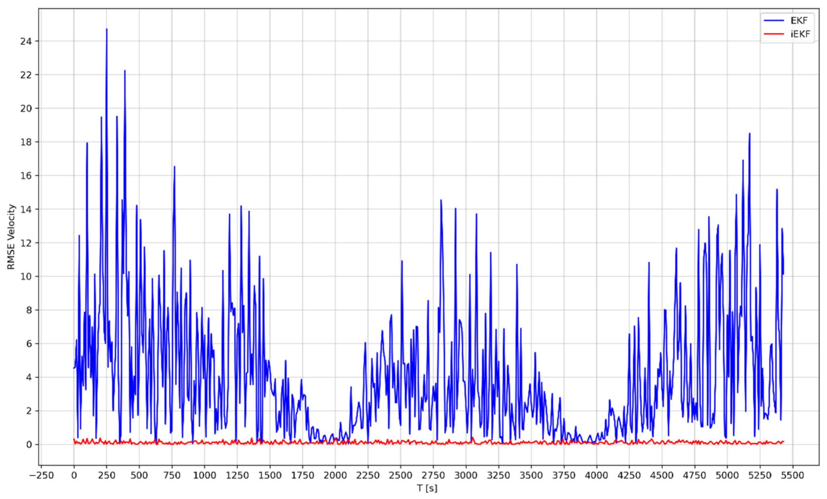
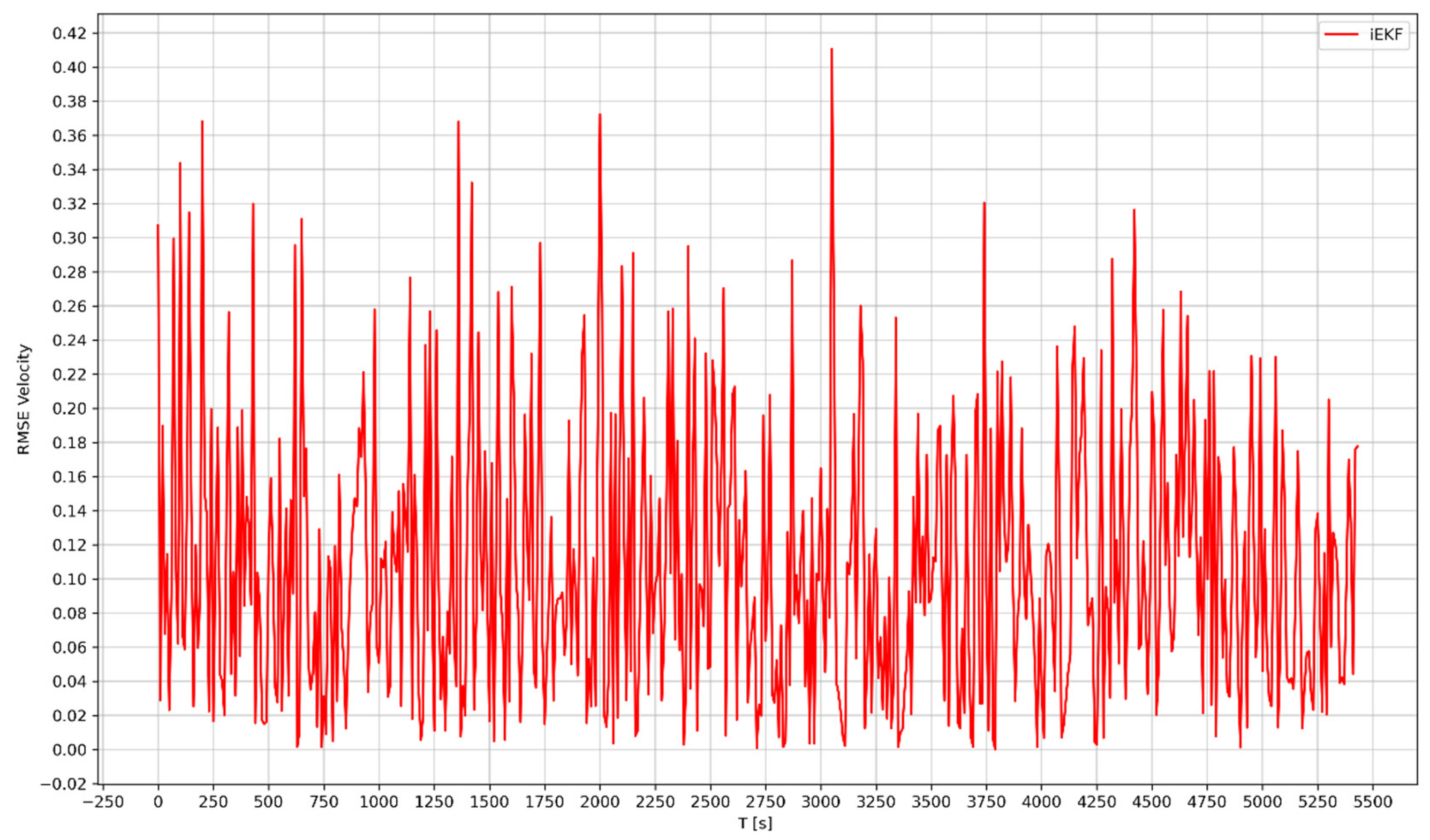
Regarding the velocity, the iEKF presents an error of less than 0.42 m/s and the EKF an error of less than 25 m/s, approximately.

By observing the graphics spikes (Figure 7 and Figure 9), it is possible to verify that the EKF holds an unstable behavior, that is, the error oscillations are higher than the iEKF. This is a very well-known behavior of EKF when dealing with highly nonlinear systems. On the other hand, iEKF maintains a more stable behavior (i.e., smaller error oscillation) (Figure 8 and Figure 10).

The spikes from Figure 8 and Figure 10 are, in general, more stable than the ones in Figure 7 and Figure 9, which means that the iEKF algorithm copes better with the nonlinearities of the system when compared with the EKF.

For the same computational time and complexity, the iEKF produces an overall superior result than the EKF.

4.2. Case 2: Orbital Maneuvers

A satellite orbit is selected beforehand depending on the mission objectives. This orbit may or may not be achievable directly from the launch. Therefore, orbital maneuvers are often required [41,42]. They are executed using onboard thrusters, typically but not always, in a sequence of short-duration bursts. However, in this paper, it is assumed that these bursts cause instantaneous change on the satellite velocity vector.

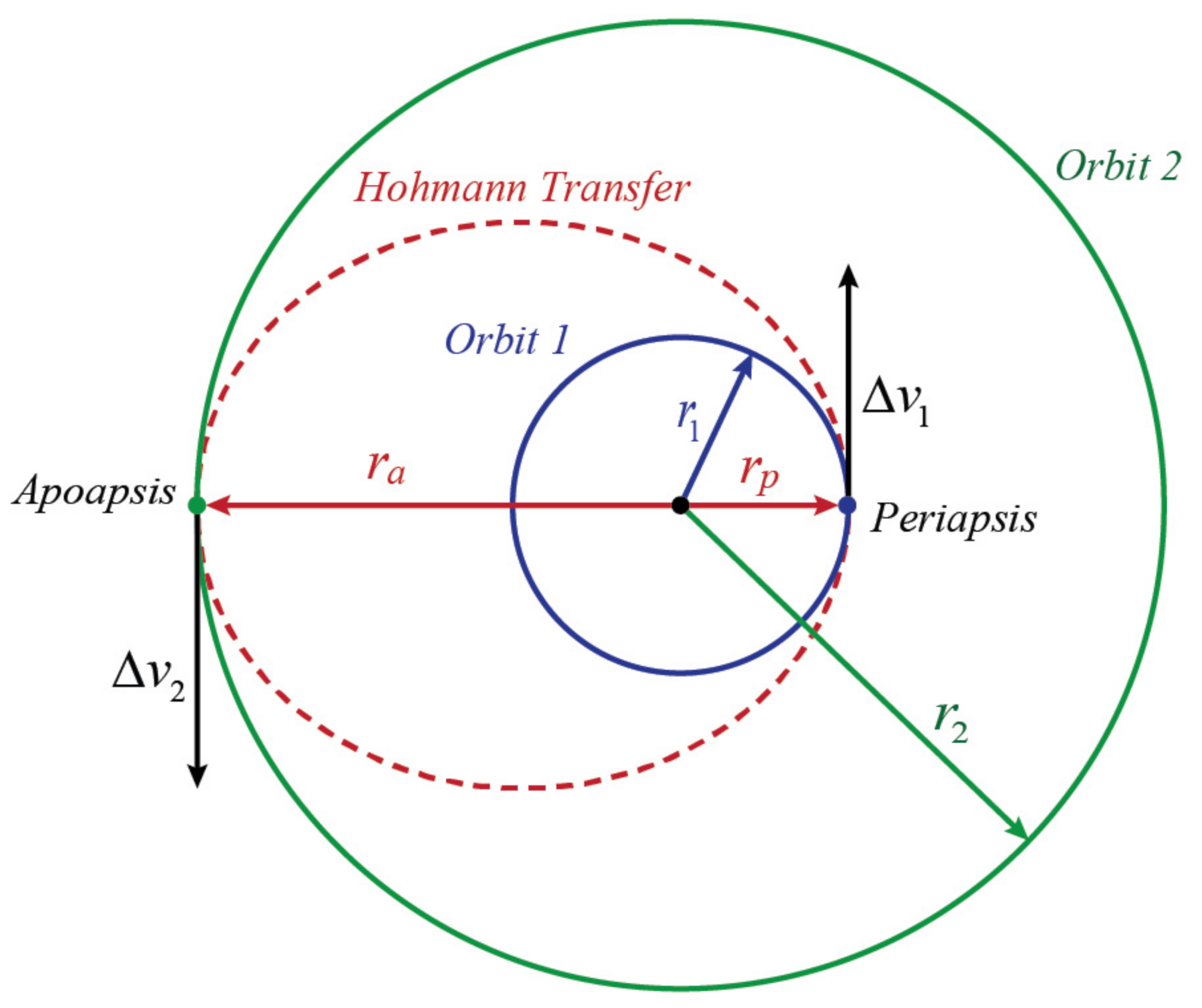
It is considered a Hohmann Transfer (HT), which is the most energy-efficient two impulse maneuvre transfer between two coplanar circular orbits sharing a common focus.

The HT consists of an elliptical transfer orbit between two circular orbits, as represented in Figure 11. The periapsis and apoapsis of the transfer ellipse are the radii of the inner and outer circles, respectively. The transfer ellipse can occur in either direction, from the inner to the outer orbit, or vice versa.

In Figure 11 $r_1=r_p$; $r_1$ represents the radius of orbit 1, and $r_p$ represents the distance between the center of the Earth and the perigee of the transfer orbit; $r_2=r_a$; $r_2$ represents the radius of orbit 2 and $r_a$ represents the distance between the center of the Earth and the apogee of the transfer orbit; $\Delta v_1$ represents the velocity change that is required to shift from orbit 1 to Hohmann Transfer orbit; and $\Delta v_2$ represents the velocity change that is required to move from the transfer orbit to orbit 2.

The semi major-axis of the transfer orbit is given by the following:

$$a_{trans}=\frac{r_1+r_2}{2}$$

(55)

In this case, $r_2>r_1$, so the first transfer occurs at the periapsis of the transfer orbit with a velocity change of $\Delta v_1$. The second transfer occurs at apoapsis, with a velocity change of $\Delta v_2$. If this second velocity change does not occur, the satellite will remain in the transfer orbit.

The velocity changes at each transfer point are given by the following:

$$\Delta v_1=\sqrt{{\mu }_{Earth}\left(\frac{2}{r_1}-\frac{1}{a_{trans}}\right)}-\sqrt{\frac{{\mu }_{Earth}}{r_1}}$$

(56)

$$\Delta v_2=\sqrt{\frac{{\mu }_{Earth}}{r_2}}-\sqrt{{\mu }_{Earth}\left(\frac{2}{r_2}-\frac{1}{a_{trans}}\right)}$$

(57)

The orbital elements considered for this case are represented in

Table 2. Orbital elements for case 2: Hohmann Transfer.

Parameter	Symbol	Value
Initial Orbit—Orbit 1
Radius	$r_1$	$3102.607 \mathrm{km}$
Orbit Eccentricity	$e$	$0$
Orbit Inclination	$i$	$0° \mathrm{deg}$
Transfer Orbit
Perigee Radius	$r_p$	$\mathrm{11,878} \mathrm{km}$
Apogee Radius	$r_a$	$\mathrm{15,878} \mathrm{km}$
Semi Major-Axis	$a$	$\mathrm{13,878} \mathrm{km}$
Orbit Eccentricity	$e$	$0.14411$
Orbit Inclination	$i$	$0° \mathrm{deg}$
Orbit Period	$T$	$\mathrm{19,921.56635} \mathrm{s}\approx 332.03 \min$
Final Orbit—Orbit 2
Radius	$r_2$	$\mathrm{11,878} \mathrm{km}$
Orbit Eccentricity	$e$	$0$
Orbit Inclination	$i$	$0° \mathrm{deg}$

.

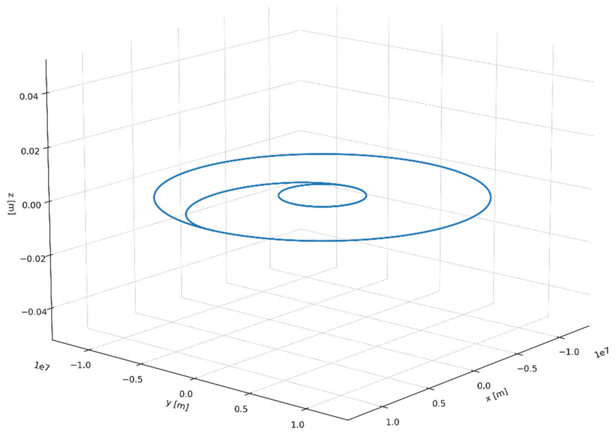
As in the previous study case, these trajectories are generated with the 4th-order Runge–Kutta (RK4) algorithm (in Python), and they are initialized with the following values:

Orbit 1:

$$\begin{array}{l}\left[\begin{array}{cccccc}r& \dot{r}& \theta & \dot{\theta }& \varphi & \dot{\varphi }\end{array}\right]=\\ \left[\begin{array}{cccccc}3.10736e+06& 4.78084e+02& 3.65140e-03& 3.65140e-03& 1.65737& -4.36388e-05\end{array}\right]\end{array}$$

Transfer Orbit:

$$\begin{array}{l}\left[\begin{array}{cccccc}r& \dot{r}& \theta & \dot{\theta }& \varphi & \dot{\varphi }\end{array}\right]=\\ \left[\begin{array}{cccccc}1.18780e+07& -1.48829e-01& 3.15396e-04& 3.15396e-04& 1.48353& 0\end{array}\right]\end{array}$$

Orbit 2:

$$\begin{array}{l}\left[\begin{array}{cccccc}r& \dot{r}& \theta & \dot{\theta }& \varphi & \dot{\varphi }\end{array}\right]=\\ \left[\begin{array}{cccccc}1.18773e+07& -4.88696e+01& 4.87456e-04& 4.87456e-04& 1.48361& 1.18892e-06\end{array}\right]\end{array}$$

The results are represented in Figure 12.

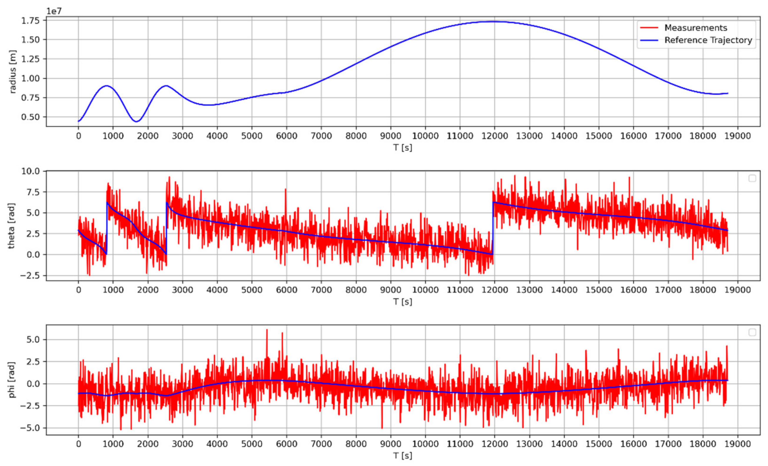
The radar tracks this orbit, and its measurements are given by Equation (6). The error standard deviations were assumed to be as follows:

$$\begin{array}{ccc}{\sigma }_r=3.16228& {\sigma }_{\theta }=1.41421& {\sigma }_{\varphi }=1.41421\end{array}$$

(58)

$$\begin{array}{cc}{\sigma }_w=9.48683& {\sigma }_v=9.48683\end{array}$$

(59)

The tracking results are presented in Figure 13.

As mentioned before, the measurement $r$ coordinate has noise as measurement $\theta$ and $\varphi$ coordinate, but since the range of this coordinate is very large, the difference between the reference and measurement is not visible in the figure.

The state vector is given by Equation (46). To initialize the filters, EKF and iEKF, we considered the following initial conditions for ${\hat{x}}_0=\left[\begin{array}{ccc}{x}_0& y_0& z_0\end{array}\right]$ and $P_0$:

$${\widehat{x}}_0=\left[\begin{array}{ccc}3.10261e+06& -1.33527e-01& -3.96816e-01\end{array}\right]$$

(60)

$$P_0=\left[\begin{array}{ccc}11.37031& 11.37031& 11.37031\\ 11.37031& 11.37031& 11.37031\\ 11.37031& 11.37031& 11.37031\end{array}\right]$$

(61)

The Jacobian matrices are given by Equation (47).

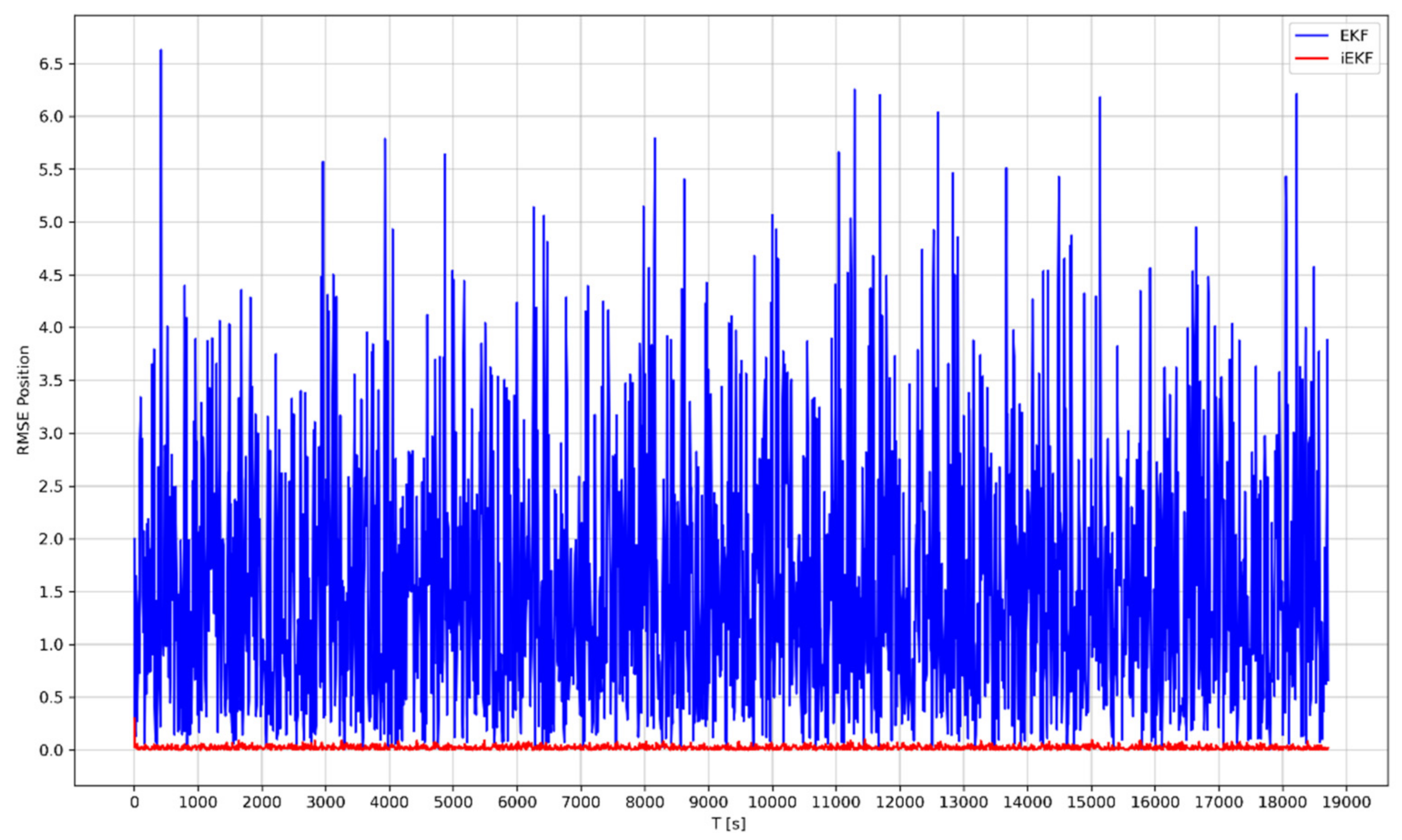
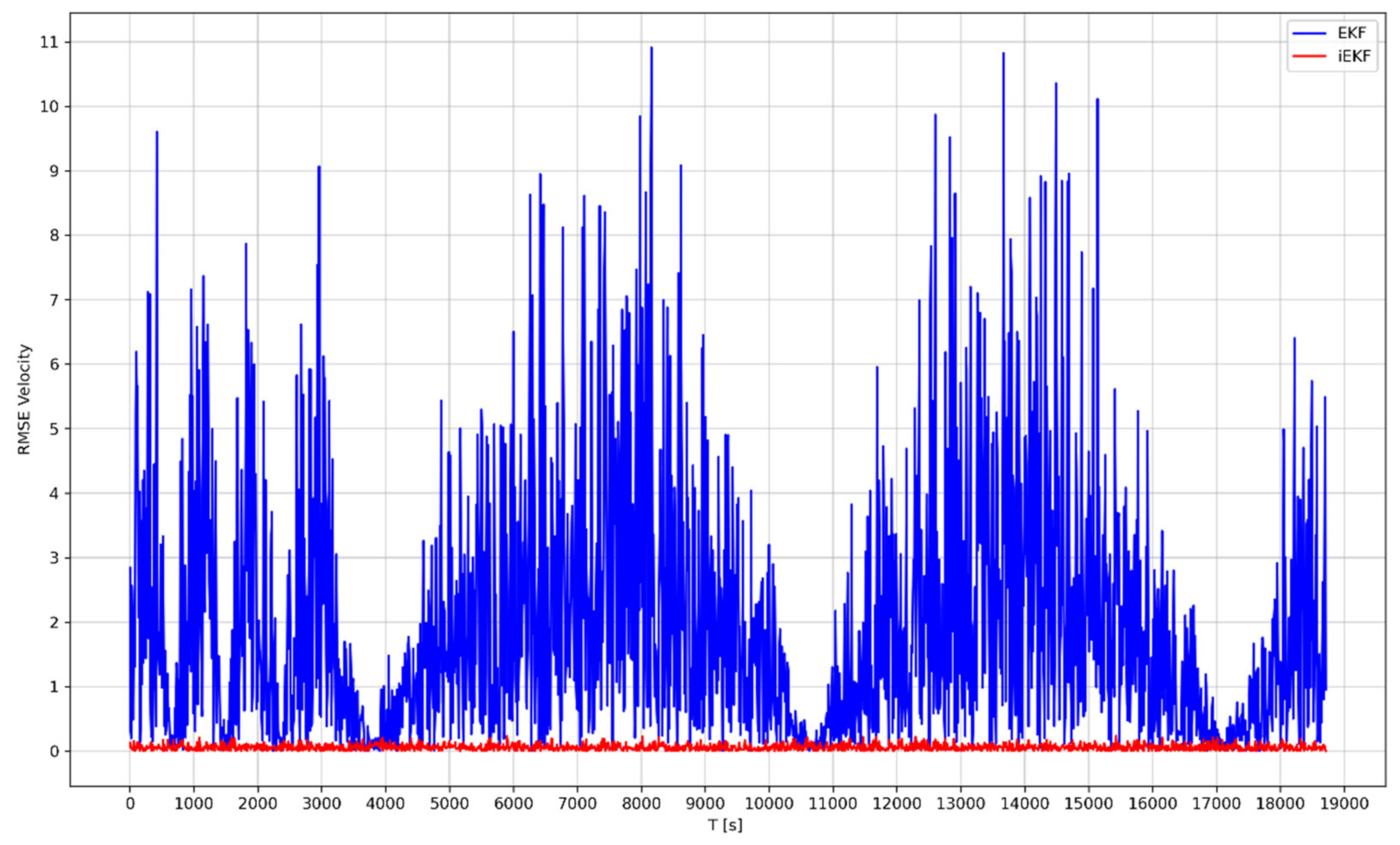
Figure 14, Figure 15, Figure 16 and Figure 17 illustrate the contrast between the EKF RMSE (blue line) and iEKF RMSE (red line) for the position and velocity.

Figure 14 and Figure 15 show that EKF RMSE for the position is less than 7 m, whereas the iEKF error is less than 0.10 m, except for the first point, which is the initial point.

The first spike of Figure 15 represents the initialization point. It is higher than the others, indicating that the (assumed) initial condition was not the most appropriate, but the algorithm rapidly overcomes it. All the other spikes are stable, which means that the iEKF algorithm copes better with the nonlinearities of the system when compared with the EKF (Figure 14, Figure 15, Figure 16 and Figure 17).

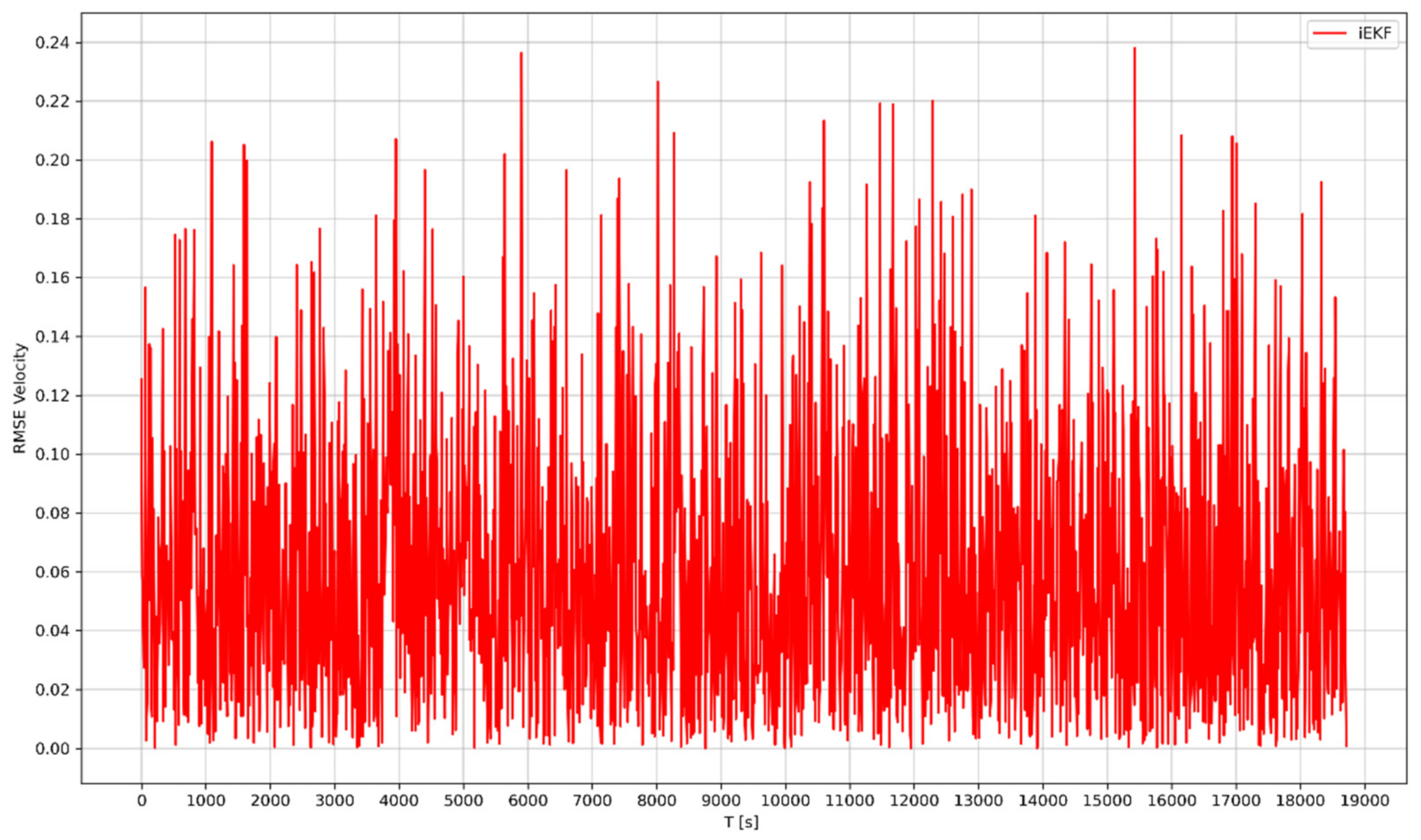
Regarding the velocity, in Figure 16 and Figure 17, the EKF presents an error of less than 11 m/s, and the iEKF presents an error of less than 0.24 m/s.

In Figure 17, it is possible to observe that the iEKF error is more stable than the EKF in Figure 16, meaning that the filter can adapt better to the nonlinearities of the model.

As it occurs in the previous study case, for the same computational time and complexity, the iEKF provides an overall superior result than the EKF.

Figure 7, Figure 8, Figure 9 and Figure 10 and Figure 14, Figure 15, Figure 16 and Figure 17 confirmed that the proposed method is more efficient in removing the ill effects of the measurement and modeling nonlinearities than the classic EKF.

5. Conclusions and Future Work

The Extended Kalman Filter (EKF) is the most widely used method to solve nonlinear state estimation in aerospace applications. However, when facing highly nonlinear models or even large initials condition errors, the EKF exhibits erratic behaviors, poor convergence and poor linearization. To address these limitations, this paper proposed an improved Extended Kalman Filter (iEKF) to solve nonlinear state estimation problem. In iEKF, it is suggested that a new Jacobian matrix calculation point and a new a priori covariance matrix computation be added to the classic EKF to improve its performance.

The proposed method was successfully validated in a realistic simulation of satellite orbit estimation and orbit transfer. The results suggest that the new modifications provide a considerably higher accuracy on the overall results, without adding complexity to the algorithm computation, when compared with the classic EKF. In summary, the iEKF is a promising method for non-linear state estimation for aerospace applications, especially radar tracking of satellite trajectories.

For future work, it is important to extend this research to other nonlinear systems with different noise conditions (for example, non-Gaussian priors). Although this simulation was realistic, it is also important to validate the method with real data of an online application.

References

- Bar-Shalom, Y.; Li, X.R.; Kirubarajan, T. Estimation with Applications to Tracking and Navigation: Theory, Algorithms and Software; John Wiley & Sons Inc.: New York, NY, USA, 2001; ISBN 978-0-471-41655-5. [Google Scholar]
- Coelho, M.; Bousson, K.; Ahmed, K. Survey of Nonlinear State Estimation in Aerospace Systems with Gaussian Priors. Adv. Aircr. Spacecr. Sci. 2020, 7, 495–516. [Google Scholar] [CrossRef]
- Raol, J.R.; Gopalratnam, G.; Twala, B. Nonlinear Filtering—Concepts and Engineering Application; CRC Press: Boca Raton, FL, USA; Taylor & Francis Group: Abingdon, UK, 2017; ISBN 978-1-4987-4517-8. [Google Scholar]
- Ristic, B.; Arulampalam, S.; Gordon, N. Beyond the Kalman Filter—Particle Filters for Tracking Applications; Artech House: Boston, MA, USA, 2004; ISBN 978-1-58053-631-8. [Google Scholar]
- Ahmed, M.; Subbarao, K. Target Tracking in 3-D Using Estimation Based Nonlinear Control Laws for UAVs. Aerospace 2016, 3, 5. [Google Scholar] [CrossRef]
- Atmeh, G.; Subbarao, K. Guidance, Navigation and Control of Unmanned Airships under Time-Varying Wind for Extended Surveillance. Aerospace 2016, 3, 8. [Google Scholar] [CrossRef] [Green Version]
- Chandra, K.P.B.; Gu, D.W. Nonlinear Filtering—Methods and Applications; Springer: Cham, Switzerland, 2019; ISBN 978-3-030-01797-2. [Google Scholar]
- Wiener, N. Extrapolation, Interpolation and Smoothing of Stationary Time Series with Engineering Applications; The MIT Press: Cambridge, MA, USA, 1949; ISBN 978-0-262-23002-5. [Google Scholar]
- Kolmogorov, A.N.; Doyle, W.L.; Selin, I. Interpolation and Extrapolation of Stationary Random Sequences; Doyle, W.; Selin, J., Translators; Bulletin of acad. Sci., Math. Series; USSR; Rand Corporation: Santa Monica, CA, USA, 1941; Volume 5, RM-3090-PR. [Google Scholar]
- Kalman, R.E. A New Approach to Linear Filtering and Prediction Problems. J. Basic Eng. 1960, 82, 35–45. [Google Scholar] [CrossRef] [Green Version]
- Grewal, M.S.; Andrews, A.P. Applications of Kalman Filtering in Aerospace: 1960 to the Present. IEEE Control Syst. Mag. 2010, 30, 69–78. [Google Scholar] [CrossRef]
- Schmidt, S.F. The Kalman Filter—Its Recognitions and Development for Aerospace Applications. J. Guid. Control Dyn. 1981, 4, 4–7. [Google Scholar] [CrossRef]
- Maybeck, P.S. Stochastic Models, Estimation and Control; Academic Press Inc.: New York, NY, USA, 1982; ISBN 0-12-480703-8. [Google Scholar]
- Welch, G.; Bishop, G. An Introduction to the Kalman Filter; University of North Carolina at Chapel Hill, Department of Computer Science: Chapel Hill, NC, USA, 2001. [Google Scholar]
- Kalman, R.E.; Bucy, R.S. New Results in Linear Filtering and Prediction Theory. J. Basic Eng. 1961, 83, 95–108. [Google Scholar] [CrossRef]
- Tanizaki, H. Nonlinear Filters: Estimation and Applications, 2nd ed.; Springer: Berlin, Germany, 1996; ISBN 978-3-662-03223-7. [Google Scholar]
- Pakki, B.C.K. Nonlinear State Estimation Algorithms and Their Applications. Ph.D. Thesis, University of Leicester, Leicester, UK, 2012. [Google Scholar]
- Julier, S.J.; Uhlmann, J.K. New Extension of the Kalman Filter to Nonlinear Systems. In Proceedings of the SPIE 3068, Signal Processing, Sensor Fusion, and Target Recognition VI, Orlando, FL, USA, 28 July 1997. [Google Scholar] [CrossRef]
- St-Pierre, M.; Gingras, D. Comparison between the unscented Kalman filter and the extended Kalman filter for the position estimation module of an integrated navigation information system. In Proceedings of the IEEE Intelligent Vehicles Symposium, Parma, Italy, 14–17 June 2004; pp. 831–835. [Google Scholar] [CrossRef]
- Zhang, X.C.; Guo, C.J. Cubature Kalman Filters: Derivation and Extension. Chin. Phys. B 2013, 22, 128401–128406. [Google Scholar] [CrossRef]
- Kulikov, Y.G.; Kulikova, M.V. The Accurate Continuous-Discrete Extended Kalman Filter for Radar Tracking. IEEE Trans Signal Process. 2016, 64, 948–958. [Google Scholar] [CrossRef]
- Kulikov, G.Y.; Kulikova, M.V. Accurate continuous–discrete unscented Kalman filtering for estimation of nonlinear continuous-time stochastic models in radar tracking. Signal Process. 2017, 139, 25–35. [Google Scholar] [CrossRef]
- Bordonaro, S.; Willett, P.; Bar-Shalom, Y.; Luginbuhl, T. Converted Measurement Sigma Point Kalman Filter for Bistatic Sonar and Radar Tracking. IEEE Trans. Aero Electron. Syst. 2019, 55, 147–159. [Google Scholar] [CrossRef]
- Ding, Z.; Balaji, B. Comparison of the unscented and cubature Kalman filters for radar tracking applications. In Proceedings of the IET International Conference on Radar Systems (Radar 2012), Glasgow, UK, 22–25 October 2012; pp. 1–5. [Google Scholar] [CrossRef]
- Kim, T.; Park, T.H. Extended Kalman Filter (EKF) Design for Vehicle Position Tracking Using Reliability Function of Radar and Lidar. Sensors 2020, 20, 4126. [Google Scholar] [CrossRef] [PubMed]
- Julier, S.; Uhlmann, J.K.; Durrant-Whyte, H.F. A New Method for the Nonlinear Transformation of Means and Covariances in Filters and Estimators. IEEE Trans. Automat Contr. 2000, 45, 477–482. [Google Scholar] [CrossRef] [Green Version]
- Arasaratnam, I.; Haykin, S. Cubature Kalman Filtering for Continuous-Discrete Systems: Theory and Simulations. IEEE Trans. Signal Process. 2010, 58, 4977–4993. [Google Scholar] [CrossRef]
- Huang, W.; Xie, H.; Shen, C.; Li, J. A Robust Strong Tracking Cubature Kalman Filter for Spacecraft Attitude Estimation with Quaternion Constraint. Acta Astron. 2016, 121, 153–163. [Google Scholar] [CrossRef]
- Gao, Z.; Mu, D.; Zhong, Y.; Gu, C.; Ren, C. Adaptively Random Weighted Cubature Kalman Filter for Nonlinear Systems. Math. Probl. Eng. 2019, 2019, 4160847. [Google Scholar] [CrossRef]
- Katzfuss, M.; Stroud, J.R.; Wikle, C.K. Understanding the Ensemble Kalman Filter. Am. Stat. 2016, 70, 350–357. [Google Scholar] [CrossRef]
- Simon, D. From here to infinity. Embed. Syst. Programm. 2001, 14, 20–32. [Google Scholar]
- Coelho, M.; Bousson, K.; Ahmed, K. An Improved Extended Kalman Filter for Nonlinear State Estimation. In Proceedings of the Aerospace Europe Conference, Bordeaux, France, 25–28 February 2020. [Google Scholar]
- Doumiati, M.; Charara, A.; Victorino, A.; Lechner, D. Vehicle Dynamics Estimation Using Kalman Filtering; John Wiley & Sons Inc.: Hoboken, NJ, USA, 2013; ISBN 9781118578988. [Google Scholar]
- Simon, D. Optimal State Estimation: Kalman, H∞ and Nonlinear Approaches; John Wiley & Sons, Inc.: Hoboken, NJ, USA, 2006; ISBN 978-0-471-70858-2. [Google Scholar]
- Zhao, Z.; Chen, H.; Chen, G.; Kwan, C.; Rong Li, X. Comparison of several ballistic target tracking filters. In Proceedings of the 2006 American Control Conference, Minneapolis, MN, USA, 14–16 July 2006. [Google Scholar] [CrossRef]
- Park, J.U.; Choi, K.H.; Lee, S. Orbital Rendezvous using two-step Sliding Mode Control. Aerosp. Sci. Technol. 1999, 3, 239–245. [Google Scholar] [CrossRef]
- Wambecq, A. Rational Runge-Kutta methods for solving systems of ordinary differential equations. Computing 1978, 20, 333–342. [Google Scholar] [CrossRef]
- Zingg, D.W.; Chisholm, T.T. Runge–Kutta methods for linear ordinary differential equations. Appl. Numer. Math 1999, 31, 227–238. [Google Scholar] [CrossRef]
- Son, E.; Lim, D.W.; Ahn, J.; Shin, M.; Chun, S. Comparison of Numerical Orbit Integration between Runge-Kutta and Adams-Bashforth-Moulton using GLObal NAvigation Satellite System Broadcast Ephemeris. J. Posit. Nav. Timing 2019, 8, 201–208. [Google Scholar] [CrossRef]
- Somodi, B.; Földváry, L. Application of numerical integration techniques for orbit determination of state-of-the-art LEO satellites. Period. Polytech. Civ. Eng. 2011, 55, 99–106. [Google Scholar] [CrossRef] [Green Version]
- Curtis, H.D. Orbital Mechanics for Engineering Students, 4th ed.; Butterworth-Heinemann—Elsevier: Oxford, UK, 2020; ISBN 978-0-08-102133-0. [Google Scholar]
- Ruiter, A.H.J.; Damaren, C.J.; Forbes, J.R. Spacecraft Dynamics, and Control—An Introduction; John Wiley & Sons Ltd.: West Sussex, UK, 2013; ISBN 978-1-11-840330-3. [Google Scholar]
Figure 1.
Radar tracking problem.
Figure 2.
Representation of the linearization point.
Figure 3.
Referential used on the satellite motion equations—spherical coordinate system.
Figure 4.
Orbital parameters of an elliptical trajectory.
Figure 5.
Three-dimensional representation of the reference satellite orbit obtain by RK4.
Figure 6.
Radar measurements of the satellite orbit.
Figure 7.
Case 1: comparison of the EKF RMSE and iEKF RMSE for the position.
Figure 8.
Case 1: iEKF RMSE for the position.
Figure 9.
Case 1: comparison of the EKF RMSE and iEKF RMSE for the velocity.
Figure 10.
Case 1: iEKF RMSE for the velocity.
Figure 11.
Hohmann Transfer representation.
Figure 12.
Three-dimensional representation of the Hohmann Transfer.
Figure 13.
Radar measurements of the orbit transfer.
Figure 14.
Case 2: comparison of the EKF RMSE and iEKF RMSE for the position.
Figure 15.
Case 2: iEKF RMSE for the position.
Figure 16.
Case 2: comparison of the EKF RMSE and iEKF RMSE for the velocity.
Figure 17.
Case 2: iEKF RMSE for the velocity.