An ALO Optimized Adaline Based Controller for an Isolated Wind Power Harnessing Unit
by
 ,
,
Amritha Kodakkal
1,†, 
Rajagopal Veramalla
2,†,
Narasimha Raju Kuthuri
1,† and
Surender Reddy Salkuti
3,*,† 1
Department of Electrical and Electronics Engineering, Koneru Lakshmaiah Education Foundation, Vaddeswaram, Guntur 522502, India
2
Department of Electrical and Electronics Engineering, Kakatiya Institute of Technology and Science, Warangal, Telangana 506015, India
3
Department of Railroad and Electrical Engineering, Woosong University, Daejeon 34606, Korea
*
Author to whom correspondence should be addressed.
†
These authors contributed equally to this work.
Designs 2021, 5(4), 65; https://0-doi-org.brum.beds.ac.uk/10.3390/designs5040065
Submission received: 19 August 2021
/
Revised: 2 October 2021
/
Accepted: 8 October 2021
/
Published: 11 October 2021
(This article belongs to the Section Electrical Engineering Design)
Abstract
:A power generating system should be able to generate and feed quality power to the loads which are connected to it. This paper suggests a very efficient controlling technique, supported by an effective optimization method, for the control of voltage and frequency of the electrical output of an isolated wind power harnessing unit. The wind power unit is modelled using MATLAB/SIMULINK. The Leaky least mean square algorithm with a step size is used by the proposed controller. The Least Mean Square (LMS) algorithm is of adaptive type, which works on the online modification of the weights. LMS algorithm tunes the filter coefficients such that the mean square value of the error is the least. This avoids the use of a low pass filter to clean the voltage and current signals which makes the algorithm simpler. An adaptive algorithm which is generally used in signal processing is applied in power system applications and the process is further simplified by using optimization techniques. That makes the proposed method very unique. Normalized LMS algorithm suffers from drift problem. The Leaky factor is included to solve the drift in the parameters which is considered as a disadvantage in the normalized LMS algorithm. The selection of suitable values of leaky factor and the step size will help in improving the speed of convergence, reducing the steady-state error and improving the stability of the system. In this study, the leaky factor, step size and controller gains are optimized by using optimization techniques. The optimization has made the process of controller tuning very easy, which otherwise was carried out by the trial-and-error method. Different techniques were used for the optimization and on result comparison, the Antlion algorithm is found to be the most effective. The controller efficiency is tested for loads that are linear and nonlinear and for varying wind speeds. It is found that the controller is very efficient in maintaining the system parameters under normal and faulty conditions. The simulated results are validated experimentally by using dSpace 1104. The laboratory results further confirm the efficiency of the proposed controller.
1. Introduction
The harnessing of wind power is a global need. The wind energy conversion industries have grown enormously in the recent past. Among the various renewable energy sources, wind power generating stations are found to be more advantageous with their eco-friendly nature, less amount carbon emissions and its cost-effectiveness.
World Energy council, in its report on ‘World Energy Scenarios Composing energy futures to 2050’, it is mentioned that the global energy demand will rise by 150%, to 53.6 billion MWh by 2050. IRENA-2018, in its report on ‘Global Energy Transformation-A Roadmap to 2050’, the emphasis is made on the increasing role of wind energy sector. According to the report, onshore and offshore wind would generate more than one-third (35%) of total electricity needs, becoming the prominent generation source by 2050.
The RECAI, based on the renewable energy investment and deployment opportunities, has placed India 4th in its index, whereas China, USA and France are ranked in the first three positions. The capital costs for wind energy harnessing are reducing with the development of technology, enabling all countries to invest in this area. This also helps the countries to expand their present capacity. According to the data of Indian Union Ministry of New and Renewable Energy (MNRE), the total installed renewable energy capacity in India has surpassed 90 GW as on 30 November 2020. The wind power segment is rated to add an additional 3000 MW with its capacity in the next fiscal.
In a wind power harnessing system, the energy of the wind is becoming converted to mechanical power and then this mechanical power is converted to electricity. It is a wind turbine that transforms the kinetic energy in the wind into mechanical energy. Gear train couples the wind turbine to a generator which converts the mechanical energy into electrical energy. The system is associated with a controller mainly to mitigate the disturbances during the loading of the generator and to maintain the system parameters in the limit. The wind energy conversion unit operation can have two approaches: The grid-connected approach helps to increase the capacity of the grid by supplementing the real power to the grid as per its demand. Standalone mode serves as an alternate source of energy in isolated places where it is not practical to extend the grid due to economic reasons.
There are many control technologies that are being used in the control of power flow in grid-connected or independent renewable energy sources. These control technologies help a power system that works on the renewable energy source to mitigate the harmonics and to avoid power fluctuations. These support the generating units to work more efficiently and make them more reliable. The control techniques can be of the conventional type or can be adaptive in nature. An adaptive algorithm adapts itself to changes that happen at the time of its run. It is based on the weight updation of the electrical signals and the error minimization. The least mean square algorithm became the most popular among adaptive algorithms, thanks to its ease of application and analysis. It was introduced mainly to simplify gradient vector calculations. The simplicity that it offers in the computation and the unbiased convergence to the optimum solution has made it very popular. Different versions of the Least Mean Square (LMS) algorithm are available. The literature survey shows that this method is predominantly used in signal processing to nullify the effect of the noise signals and to filter out the noises from the signals. Many noise signals which cannot be removed using traditional filters are easily removed by using this adaptive algorithm. It is found that the normalized LMS algorithm creates the drifting problem. Drifting is a situation where the weight updation in LMS goes unbounded, as a result of inadequate input values. A leaky factor that is introduced, solves the problem. A variable-weight, variable step, least mean square algorithm is an improved version, which helps to improve the convergence rate of the algorithm. By adjusting the values of the leaky factor and the step size, the convergence rate can be improved.
Many articles were reviewed in this work. The design, control, performance and testing of electrical generators are explained in [1]. The sources and effects of harmonics, measurement, analysis and compensation of the same and the recommended practices of the utilities in dealing with the same, are dealt in the reference [2]. The LMS algorithm is applied by many researchers in different applications. The general nature of the LMS algorithm with its derivation and advantages are given in [3]. Study and implementation of seventeen of the best known LMS algorithms and their comparison on the practical aspects based on the study is carried out in [4]. The LMS algorithm is applied to an isolated hydropower station for the regulation of voltage and frequency, then a leaky factor is introduced and a further modified version is used to control the behavior of a Synchronous Reluctance Generator and in active noise control [5,6,7,8,9]. A new model is introduced to tackle the issue of the low convergence rate of the leaky algorithm [10]. In this model, the sum of exponentials of the error with a leakage factor is used as the objective function. Different traditional and adaptive and Artificial Neural Network (ANN) based control techniques are reviewed [11,12]. Implementations of different versions of adaptive algorithms in different filters for power quality improvement are proposed in [13,14,15,16]. A comparative study on hybrid Machine Learning methods which are used to classify the power quality disturbances is carried out in [17]. A controller for extracting maximum power from the wind energy converting system is given in [18]. The reasons for the reduction in power system stability when renewable energy sources with power electronic converters are integrated with the grid and its effect on the flexibility of the power system, challenges and opportunities and the need for detailed stability studies to be carried out, to have a stable grid system in the future are reviewed [19,20,21,22]. Control of hybrid energy systems is discussed [23,24]. Different control techniques for filters for power quality improvement are studied and analyzed [25,26,27,28,29]. A wind power generating unit using ANN control used for a PMSG is proposed in [30]. Stability, Reactive power management, Reliability and Quality while integrating wind power systems to the Grid are discussed in [31,32,33,34,35]. Reference [36] defines and proposes measures to illustrate the variations of powers and power flows. It also presents methods to improve energy quality and highlights research directions on energy quality.
The reviewed literature in the LMS algorithm have not mentioned any method to determine the value of the leaky factor and is assumed to be calculated through trial-and-error methods. Reference [4] reviews different complex methods for the calculation of step size for different applications.
This paper uses optimization techniques to find the values of the step-size, leaky factor and the controller gains which avoid the lengthy process of experimenting with different numbers. Here three different optimization techniques are used and the results are compared. Particle Optimization algorithm, Whale Optimization and Antlion Optimization are techniques that are widely used for various applications. Here, these methods are implemented to find the controller gains, leaky factor and step size. From the comparison of the results obtained, the Antlion optimization technique is found to be the most efficient in minimizing the frequency error and the terminal voltage error and for maintaining constant values of voltage and frequency, and in retaining the best stability for the system.
2. Wind Energy Characteristics
The wind which is caused due to the uneven heating up of the surface of the earth is captured by the wind turbines and becomes converted to electrical energy. The power output delivered by the wind turbine depends on the wind speed and the turbine radius. It is impractical, rather impossible, to convert all the wind energy which strikes the wind turbine blade, to the output electrical energy, as the conversion of 100% input kinetic energy means that the output wind has zero kinetic energy, which is not possible Thanks to the development of technology, the efficiency of a wind turbine is improved to around 50%.
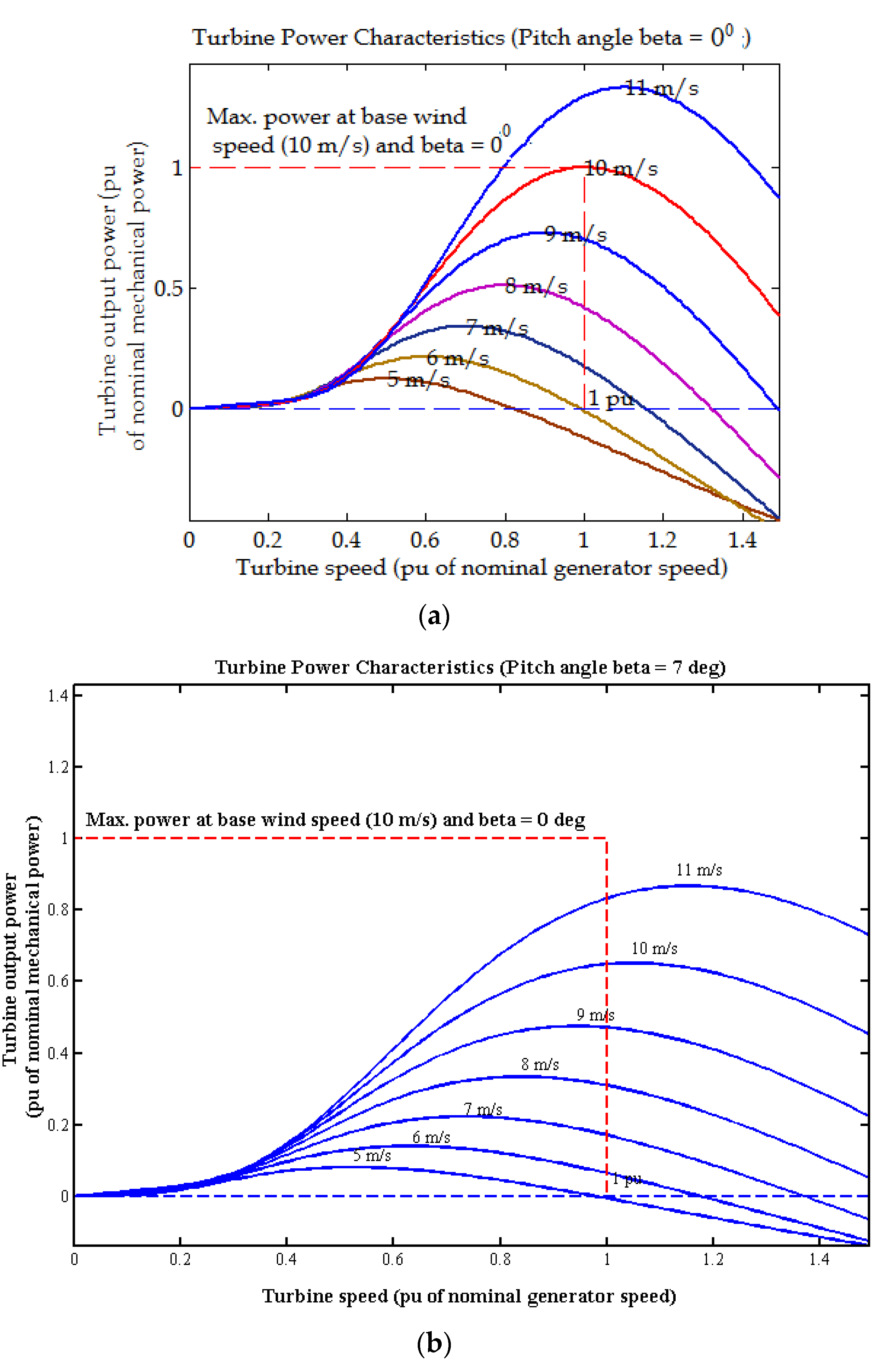
The turbine output varies with the speed of the turbine. The graph in Figure 1 is a direct catch from the wind turbine characteristics from Simulink. This shows how the turbine output varies with the speed of the turbine for different wind speeds. It also shows the effect of pitch angle in the turbine output. Pitch angle is the angle at which the turbine blade is aligned with respect to the plane of rotation, so that the generated power output is maximum, at a particular wind speed. Figure 1a shows the turbine characteristics when the pitch angle is zero. When the pitch angle is increased to 7°, the power output decreases, as shown in Figure 1b. Here, in the wind turbine under study, the maximum output is generated with zero pitch angle.
For low wind speeds, the generated output power is less. As the wind speed increases, the generated power increases. Corresponding to a particular value of wind speed, there is a maximum power that can be generated by the turbine. After this point, a further increase in turbine speed will cause a decrease in the generated power.
3. System Configuration
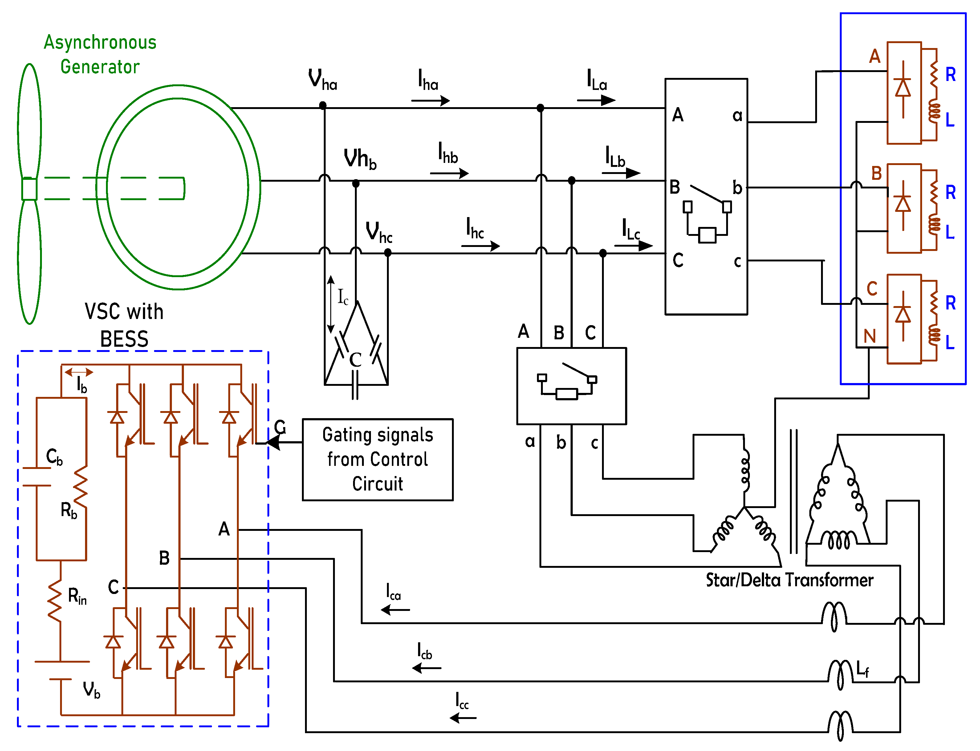
The wind energy harnessing unit under study uses an asynchronous generator with four poles, having a rating of 7.5 kW, 415 V and 50 Hz. An excitation capacitor that is delta connected and having a reactive power capability of 8 kVAr supplies the reactive power required for magnetization. A controller is configured which produces the triggering signals for the IGBTs which are the switching devices in the voltage source converter. A Star—Delta transformer of 7.5 kVA, links the controller with the generating unit and the load. The star-delta transformer helps to reduce the rating of various components of the controller and helps the battery energy storage system (BESS) to operate at a lower voltage level.
The neutral terminal of the load is connected to the transformer neutral. Any disturbance in the balanced operation of the load produces a current which flows through the neutral wire. The above arrangement provides a closed path for this unbalanced current through the transformer neutral, which helps the source current not to become affected. Thus, the source neutral current continues to be zero even during load unbalance because of the transformer. The schematic of the Wind power unit is given in Figure 2.
The battery energy storage system maintains a constant dc voltage at the bus and it helps to compensate for the uncertain effects of variable wind speed and any change in load. The BESS absorbs the excess amount of active power when the power handled by the load is less than the generated power. In a similar way, when the power required at the load is more than the generated power, the battery releases the stored energy to support the generator. This helps to keep the frequency constant. The ripples in the battery current are removed by connecting an inductor in series. Any fluctuations in the load or the wind speed will normally have an effect on the source current which is not desirable. These irregularities are taken care of by the controller by providing the necessary compensating current to the induction generator from the inverter. The inverter switching devices work based on the gating signals generated according to the error between the current reference values and the actual values sensed. The reference signals are produced based on the weight updation in the system. The weights are calculated in each phase and the average of it is combined with the frequency error signal to calculate the direct component of the reference current, whereas it is combined with the error produced in the terminal voltage, to produce the quadrature component of the reference current. This helps the PCC voltage and frequency to stay within the allowed limits even when there are changes in the consumer loads and also during the variation in wind speeds.
The dc-link potential is controlled by the battery voltage Vb. The value of Vb is related to the line to line voltage VLL as per the given equation
where ‘m’ is the modulation Index and is assumed as 1. A delta-connected excitation capacitor unit is connected to stream the reactive power required to generate the necessary phase voltage by the induction generator. An AC inductor is connected mainly to reduce the ripple.
4. The Control Technique
The control technique used is the least mean square which is the most popular in the Adaline algorithms. LMS technique is a novel adaptive algorithm that is centered on the method of steepest descent. This is an ANN-based technique that is found to be simple and robust. LMS algorithm involves easy computations avoiding complexity involving gradient calculations and matrix inversions. The algorithm performance is evaluated based on its capability to retain the frequency and the terminal voltage during the normal and also during the fault conditions. Many iterations are carried out to update the weight vector so that the mean square error is the minimum. The weight updation is carried out on every iteration based on which the controlling action is performed. A slightly modified version of the LMS algorithm is used here which includes an optimized step-size and an optimized value for the leaky factor in the determination of the weight. The Leakage factor is included to solve the drift in the parameters which is considered as a disadvantage in the normalized LMS algorithm. This drift is caused mainly due to the inadequate input sequence. This causes instability as the algorithm produces unbounded output for a bounded input. The leaky factor takes only a part of the weight to be appropriately added to find the new weight which helps in mitigating the drifting problem.
The step size is an inherent characteristic of the LMS algorithm and should be carefully chosen. A large value of step size is required for faster convergence, but it results in a large error and loss of stability. On the other hand, small step size reduces the error, improves the stability, but increases the convergence rate [4]. Thus, the value is selected such that it makes a balance between the accuracy and the rate of convergence.
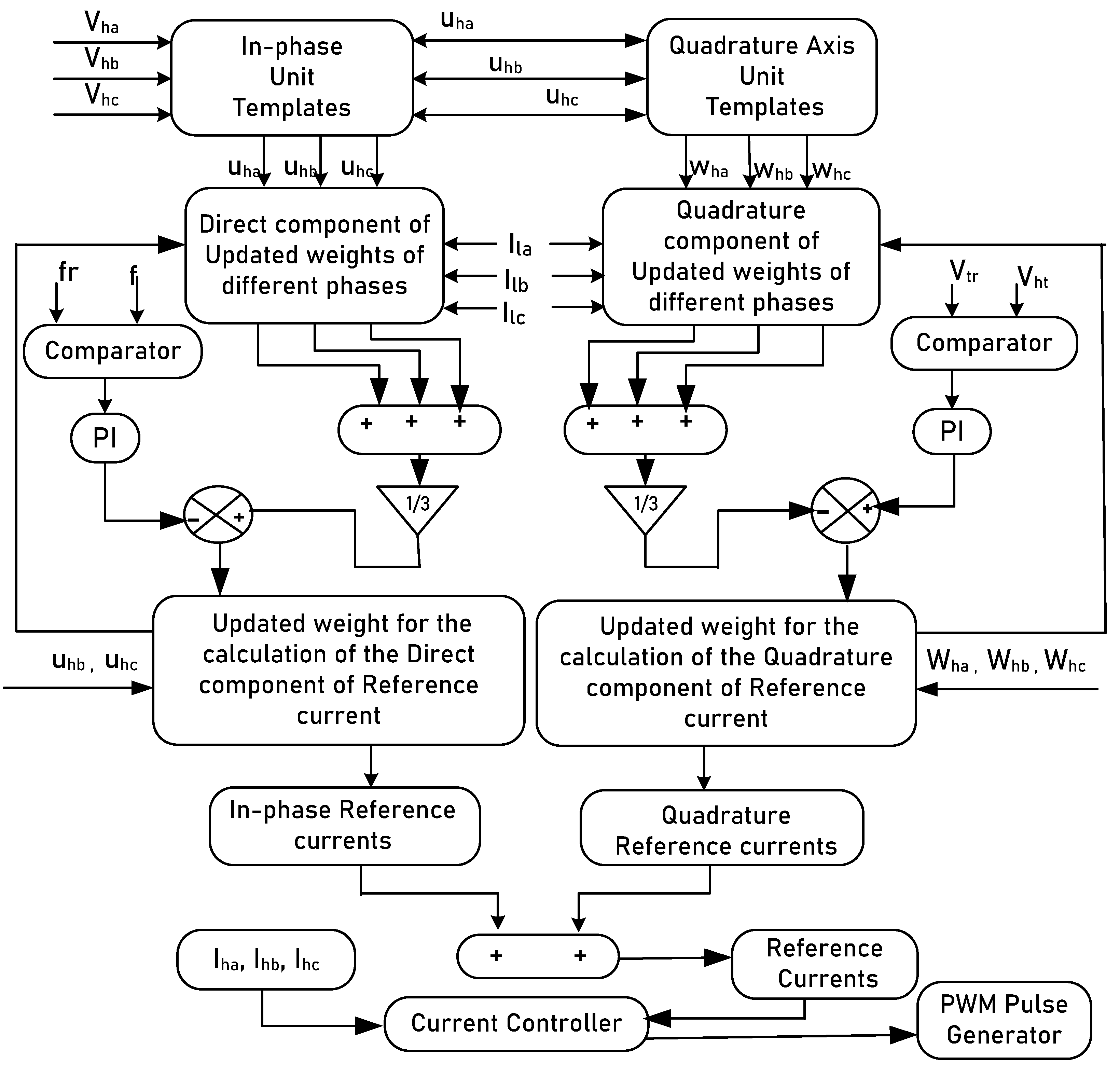
The flowchart which explains the controlling action through the Leaky LMS is given in Figure 3. The components of the reference currents are produced based on the online modification of the weights. The direct component of the reference current is calculated taking the frequency error into account and the calculations for the quadrature component are carried out taking the difference between the reference voltage and the terminal voltage into account.
4.1. Estimating the Direct Component of Reference Currents
The potential at PCC is calculated from voltages (, and ) as,
, and are the unit vectors which are in phase with phase voltages , and .These are expressed as,
The frequency of the alternating current is measured as factual and compared with the standard frequency fref and the error signal is duly modified with the Proportional Integral (PI) controller gains to generate the output signal.
The error of the frequency controller at the pth sampling instant is
At the pth sampling instant, the PI controller gives out an output which is given as,
Kpd is the gain of the proportional controller and Kid is the gain of the integral controller.
In the direct component calculation, the weights of the load currents in each of the three phases are estimated individually as,
μ is known as the step size or the convergence factor. The convergence rate and accuracy of estimation are decided by this value. The value of μ is selected such that it makes a compromise between the accuracy and convergence rate. The observed practical value of μ ranges between 0.05 and 0.5. β is the Leakage factor and its value is found to work in the best way when its value is less than 1.
The mean of the total weight is integrated with the modified frequency error or loss component of power, to acquire the modified weight.
The modified weight of the in-phase component of the reference is expressed as,
The direct component of the reference value of source currents are computed as,
4.2. Estimating the Reactive Power Component of Reference Currents
The unit vectors which are in quadrature with voltages , and are derived from the unit values , and as,
At every instant, the reference value of voltage is compared with the sensed value of the terminal voltage. The error at the pth sampling instant is given as,
where is the reference value of terminal voltage and is the value of the ac voltages measured at the source terminals at the pth instant.
In the quadrature component calculation, the weights of the load currents in each of the three phases are estimated individually as,
The modified weight of the quadrature component of the reference current is given by,
where is the output of the PI controller which measures the error between the terminal voltage and the standard value at the th instant and is given by,
The quadrature components of the reference currents are given by,
4.3. Estimating Reference Values of the Source Currents
The reference values of the harnessed currents are determined as:
The reference values of currents , and are compared with the measured values of the currents , and and an error value is generated. Taking this current error as input, the current controller produces the signals for the switching operation of IGBTs in the inverter.
5. Optimization Technique
There are many optimization techniques used for optimizing different parameter values. In this paper, values of the variables are optimized using three dominant meta-heuristic approaches—Particle Optimization algorithm (PSO), Whale Optimization (WOA) and Ant Lion Optimization (ALO). Seyedali Mirjalili developed Antlion Algorithm and Whale optimization algorithm. Particle swarm Optimization is introduced by Bruno and Victor as a powerful tool for the solution of engineering problems. The evolution, features and validation of these three techniques are clearly mentioned in [37,38,39]. Different optimization methods for power quality and transient stability are discussed in [40,41,42]. The optimized values of controller gains, leaky factor and the step size are determined by these techniques. The values obtained are substituted and observed in the output waveforms. The optimized values from ALO are found to be the most suitable and were giving excellent output waveforms which are shown in the results.
Particle Swam Optimization (PSO) is one of the most robust population-based techniques which is based on the intelligent movement of bird flocks. The basic concept of PSO lies in accelerating each particle towards its self-best position and global-best position obtained by it so far with a random weighted acceleration at each time step. The particle should be initialized with random position and velocity vectors. Then it searches for optima by updating generations. The fitness value is calculated in every iteration and each particle is updated by its personal best (pBest) and the global best (gBest) values. The particle updates its velocity and position in each iteration, based on the obtained values. Its simplicity in implementation, freedom from derivatives and reduction in a number of parameters have made it very popular and is considered an efficient global search algorithm.
The Whales Optimization Algorithm (WOA) is also a nature-inspired algorithm. This is a recently introduced one. It is based on the bubble-net hunting strategy of humpback whales. In fact, the incredible nature of the spiraling of humpback whales has taught scientists the ways to reduce the drag in the wind turbine blades. More study on the hunting mechanism of these whales resulted in developing WOA. The mathematical modelling is based on the shrinking encircling and spiral updating around the prey. The position of the search agent around the possible solution is updated in every iteration.
The Ant Lion algorithm is based on the hunting mechanism of antlions. Antlions dig pits to trap the ants. The ants which have a random walk around the pit become entrapped inside. The position and the fitness of the ants and the antlions are updated in each iteration. Once the antlion catches the prey, its fitness will be assigned to the antlion. This process continues till the best optimum value is obtained.
These three methods are proven to be very efficient in solving single as well as multi-objective functions. These were applied to the LMS Simulink model for 2 purposes. The proportional and integral controller gains were found out by using these 3 techniques. In addition, the same techniques were used to determine the values of the step size and the leaky factor. The results show that the Antlion algorithm gives the best results in terms of the convergence rates, the controller gains and the step-size and the leaky factor values. Substitution of these values in the simulated circuit proved that the values obtained by the Antlion optimizer work the best with this circuit.
5.1. Objective Function
The objective function is defined as a minimization problem for minimizing the steady-state errors of frequency and terminal voltage.
where,
5.2. Constraints
0 < Kp1 < 5; 0 < Ki1 < 5
0 < Kp2 < 4; 0 < Ki2 < 4
6. Results and Discussion
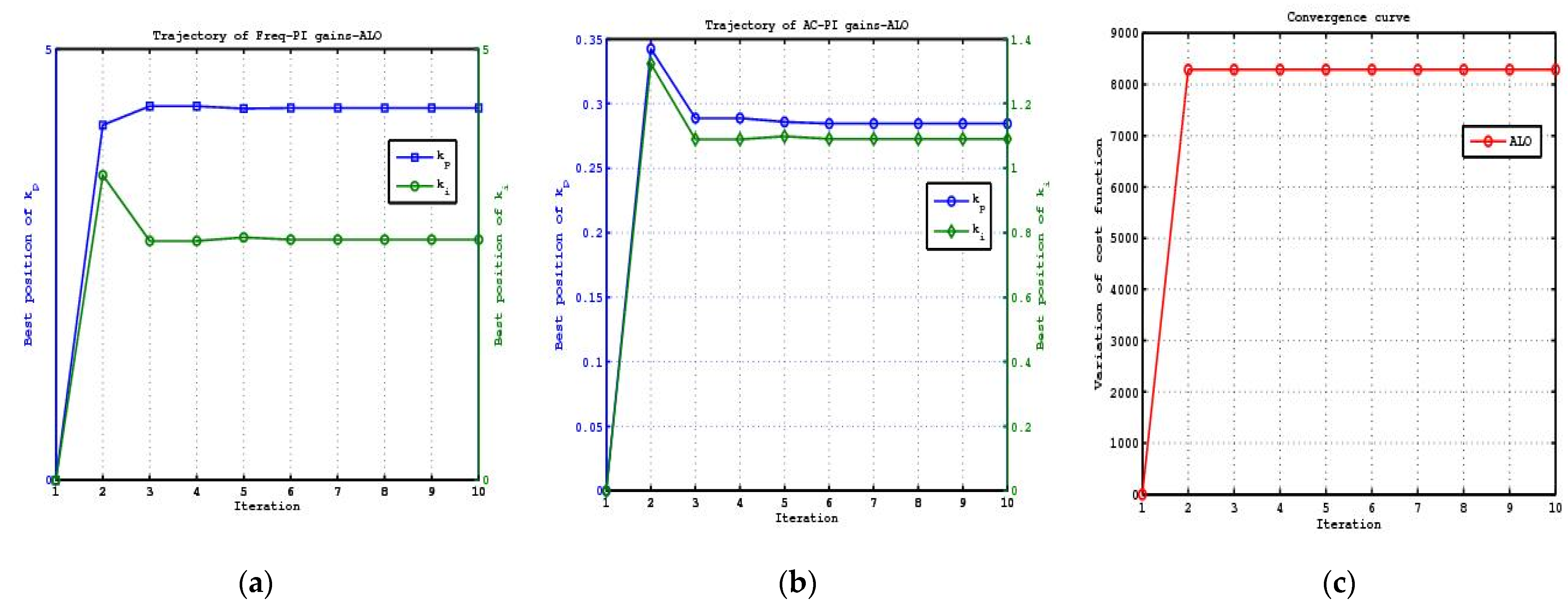
Figure 4, Figure 5 and Figure 6 show the results of the application of ALO, PSO and WOA to the circuit to find the frequency and AC gains for the control algorithm which is used to stabilize the system under study.
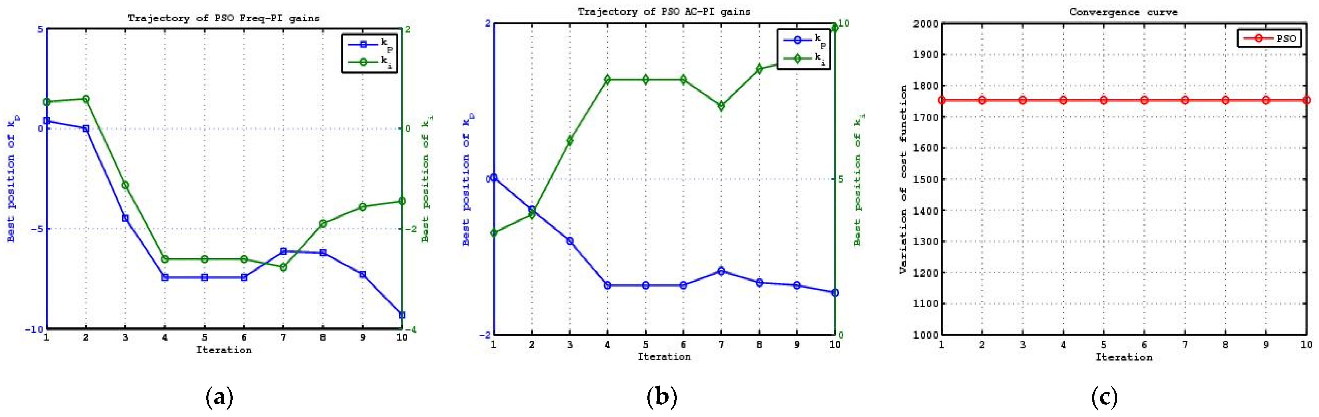
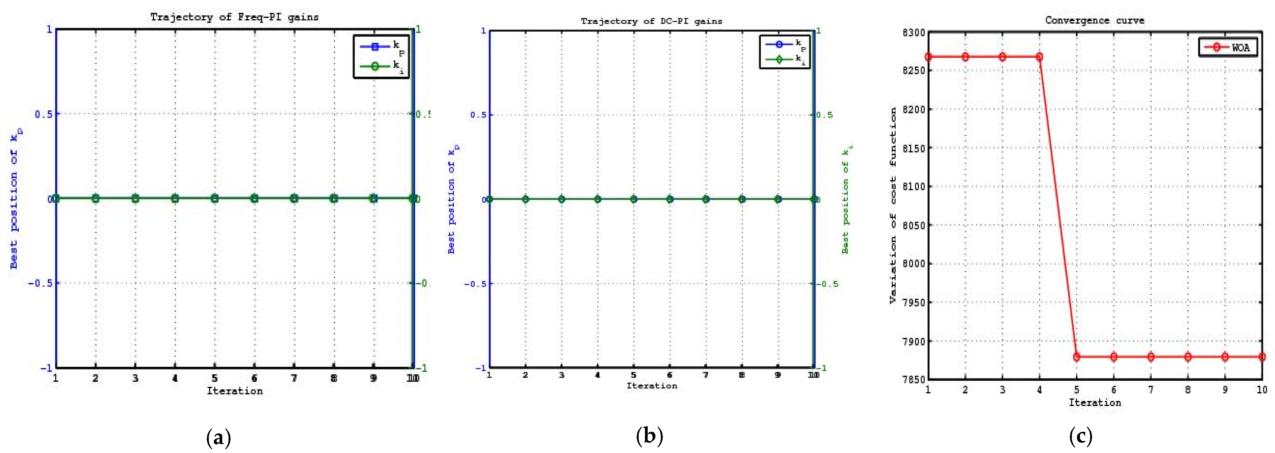
From the graphs shown, it is very clear that PSO and WOA have difficulty in converging to the final value. However, the results of ALO show that the rate of convergence is smooth and fast. The gains are becoming stabilized in the minimum number of iterations. The values of the gains obtained from ALO, when substituted to the Simulink model gave the best stability to the system during fault conditions and changes in the wind speeds.
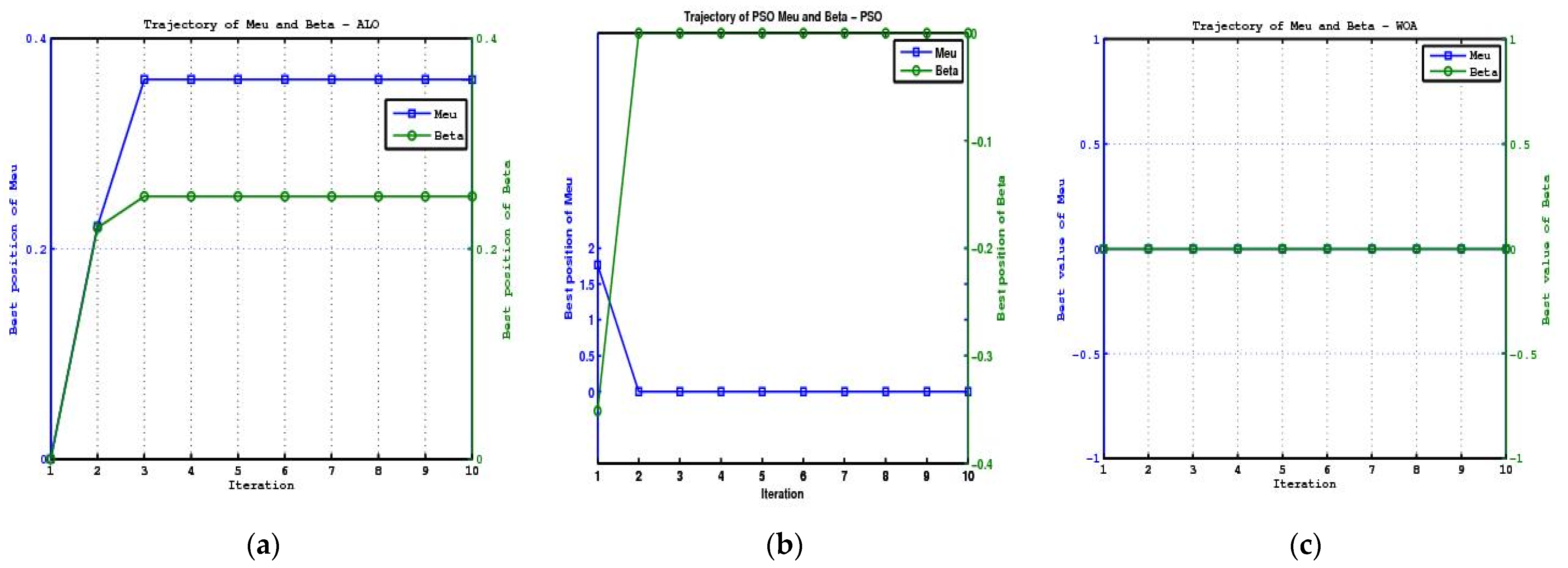
The optimization techniques when used to find the step-size and leaky factor gave a similar result. Figure 7 shows the results of the application of ALO, PSO and WOA to the circuit to find the step size and the leakage factor for the control algorithm which is used to stabilize the system under study. These values are directly substituted in the control algorithm to acquire the output and the values obtained from ALO are found to be the most suitable for the proposed controller.
The values are shown in the tabular form in Table 1 for the purpose of comparison.
The results show that the Antlion algorithm gives very good results in terms of the convergence rates, the controller gains and the step-size and the leaky factor values. Substitution of these values in the simulated circuit proved that the values obtained by the Antlion optimizer work the best with this circuit to give the best stability to the system during fault conditions and changes in the wind speeds.
7. Simulation Results
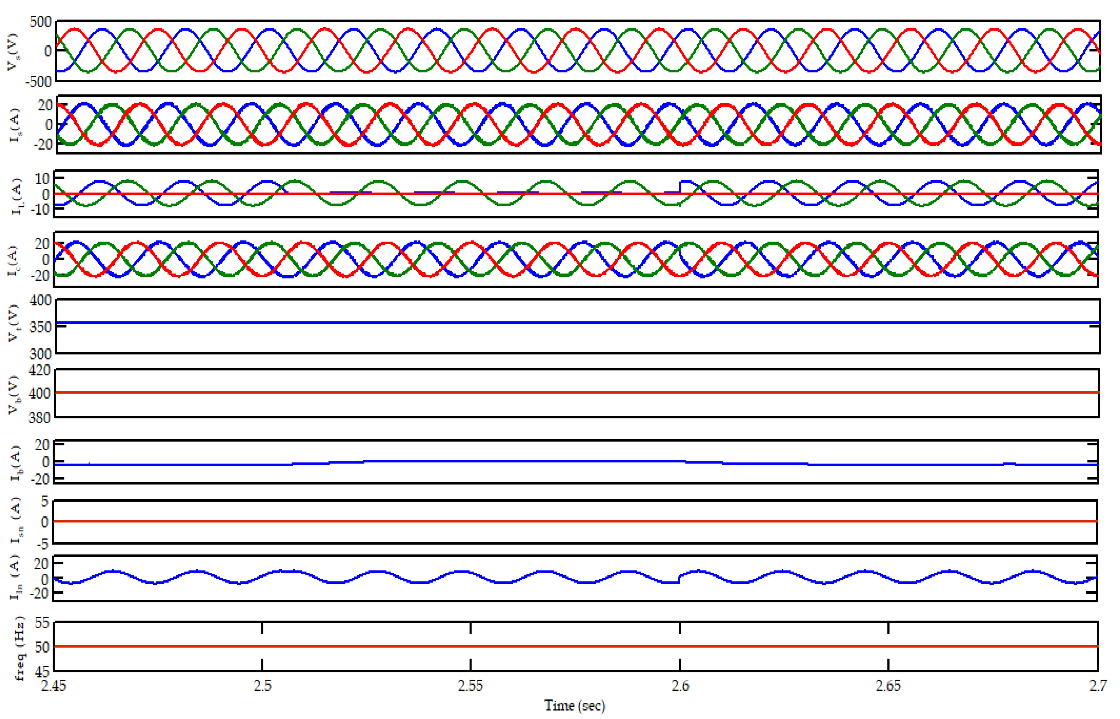
The Wind energy conversion unit is simulated using the Sim-Power System toolbox in MATLAB/SIMULINK(2009a version, Mathworks, Natick, MA, USA). The unit uses an induction generator for energy production. The harnessed voltage, source current, current at the load terminal, terminal voltage Vt and frequency were studied with different types of load conditions and wind speeds. The wind generator begins to develop an output voltage at 0.3 s. The load is connected to the system at 0.35 s. The controller is connected at 0.5 s. The controller action is tested for different loading conditions—linear and nonlinear. The controller is found working perfectly in regulating the voltage and frequency in the negligible time period in both cases. The load was disconnected in one of the phases at 2.5 s, creating an unbalance; then the same load was reconnected at 2.6 s. The controller action was very quick to regain the balance of the circuit. The source currents were unaffected during this time period due to the efficient operation of the controller in maintaining the voltage and frequency of the circuit.
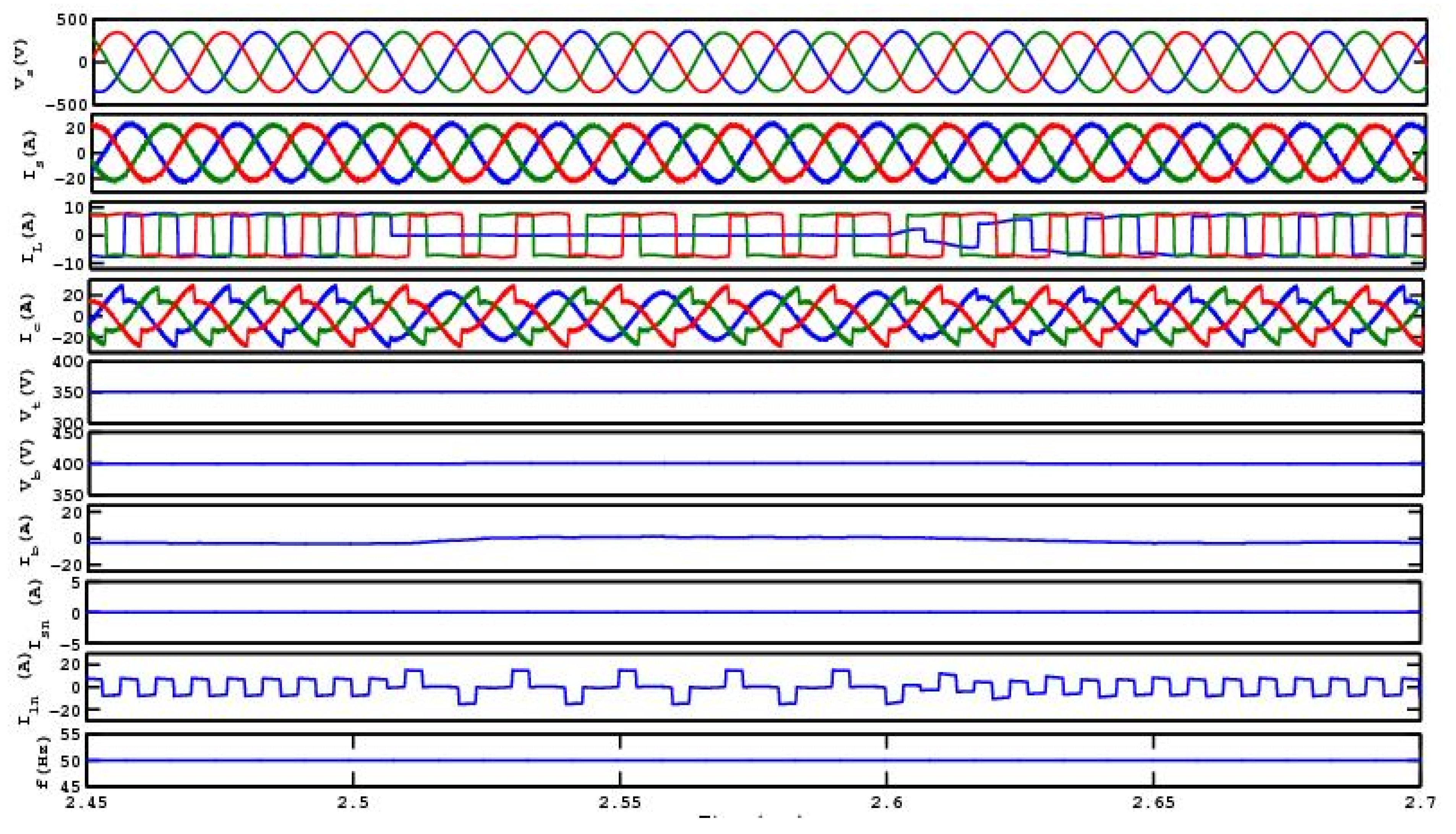
Figure 8 shows the characteristics of the source voltage, source current, load current, controller current, terminal voltage, DC link voltage, battery current, frequency, neutral line current of the generator and the load neutral current of the generator with linear loads when the wind speed is constant.
The graphs show the variations in the above-mentioned quantities when the load is removed in one phase at 2.5 s. It is found that the controller very effectively maintains the source currents at a constant level, during normal and faulted load conditions. From the graph, it is clear that the current in the battery is positive when the load was disconnected, which indicates that the battery is charging. The extra power which was not used by the disconnected load is absorbed by the battery. Thus, the battery helps to maintain the voltage and frequency constant in case of any fault condition. The load unbalances cause a neutral current to flow. Since the load neutral is connected to the transformer neutral point, the current caused by the unbalance circulates in between the load neutral and the transformer neutral. The source neutral current is found to be unaffected and this happens due to the presence of the Star-Delta Transformer.
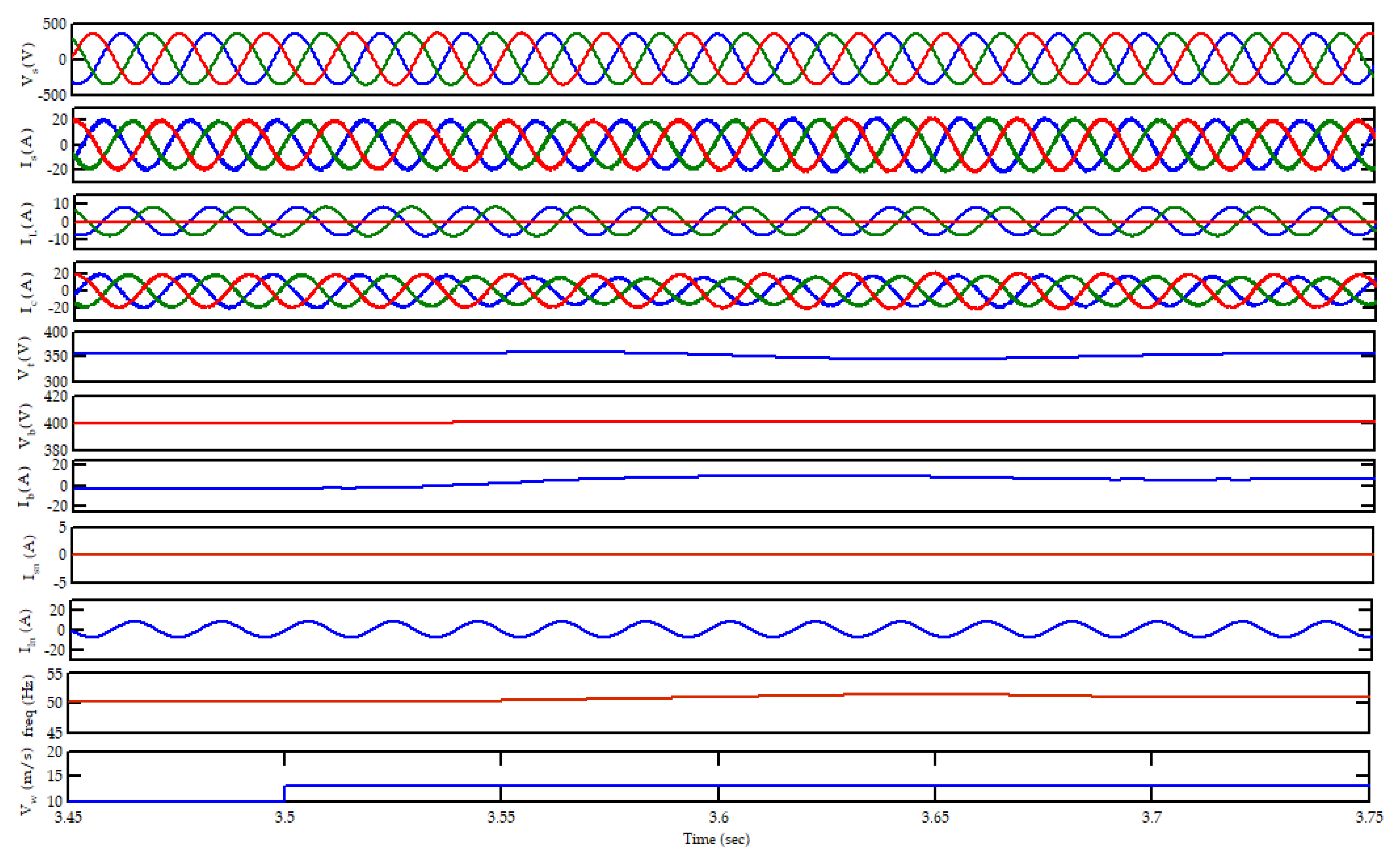
Figure 9 shows the characteristics of the source quantities and load quantities, controller current, terminal voltage, DC link voltage, battery current, frequency, neutral line current of the generator and the load neutral current of the generator with nonlinear loads when the wind speed is constant.
Figure 10 shows voltage and current at the source side for a linear load, when the wind speed changes. Wind speed changes from 10 m/s to 13 m/s at 3.5 s. After a moment of instability, the system comes back to its normal operation. Frequency and the PCC voltage come to their standard value. When the wind speed increases, the reactive power absorbed by the system increases, which causes the terminal voltage to drop. The frequency increases. The controller acts quickly to mitigate these variations. All the variations are suppressed and the stability is maintained by the controller. The terminal voltage and the frequency are brought back to their standard values very quickly by the controller. The battery current increases as the battery will try to absorb the extra power generated. The source neutral current remains zero, as the load neutral current completes its path through the transformer neutral.
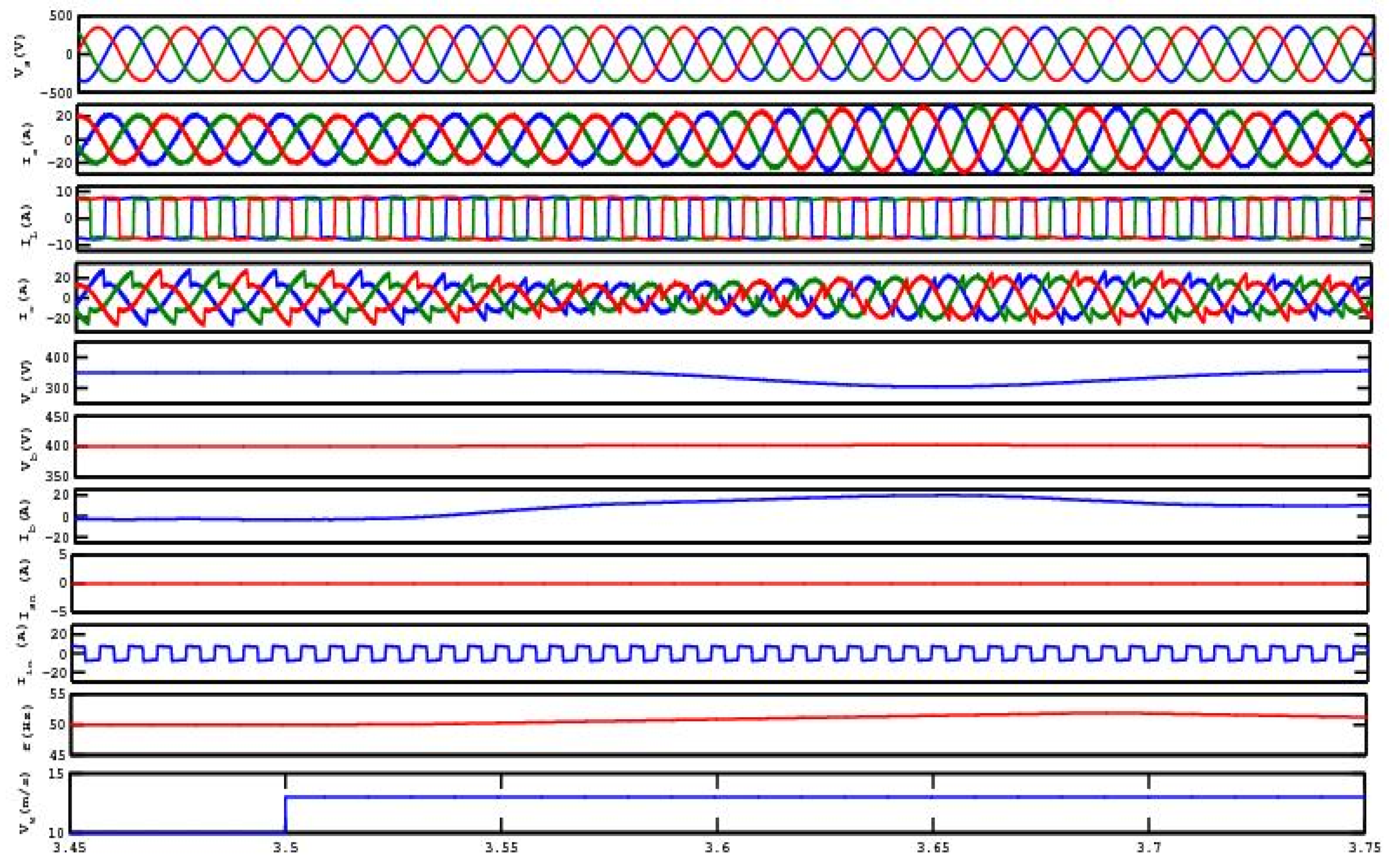
Figure 11 shows the effect of wind speed change in the operation of the wind power unit when it supplies to a nonlinear load.
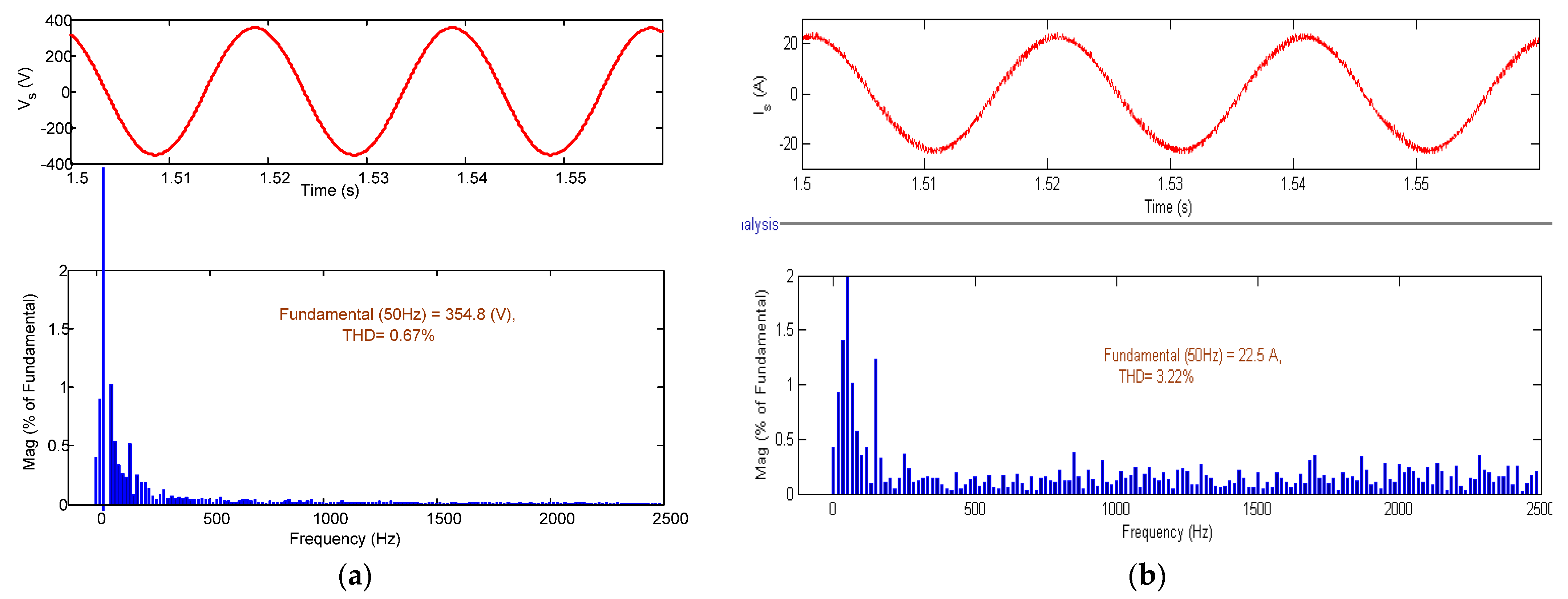
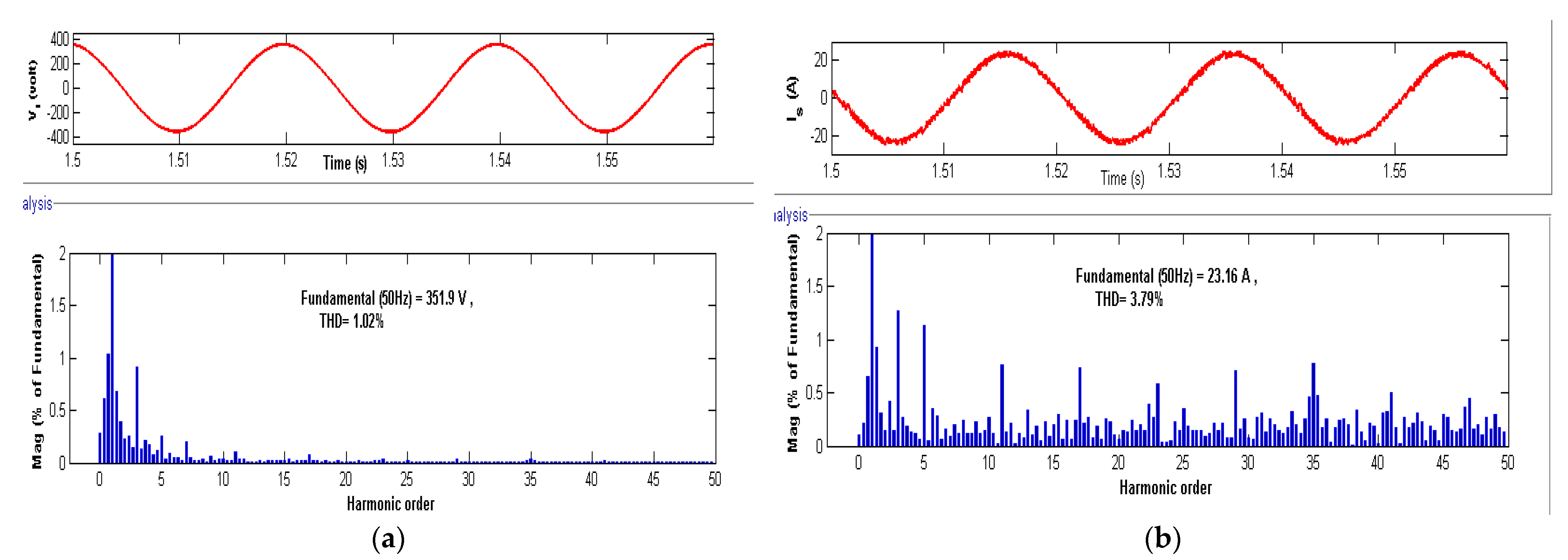
The Total Harmonic Distortion (THD) values of the voltage and current of source with nonlinear load are shown in Figure 12a,b. THD values are plotted against the frequency here. The total harmonic content in the source voltage is found to be 0.67%. For the source current, THD is found to be 3.22%. These values are well within the range specified by IEEE 519 standards. Figure 13a,b show the THD plotted against the harmonic order.
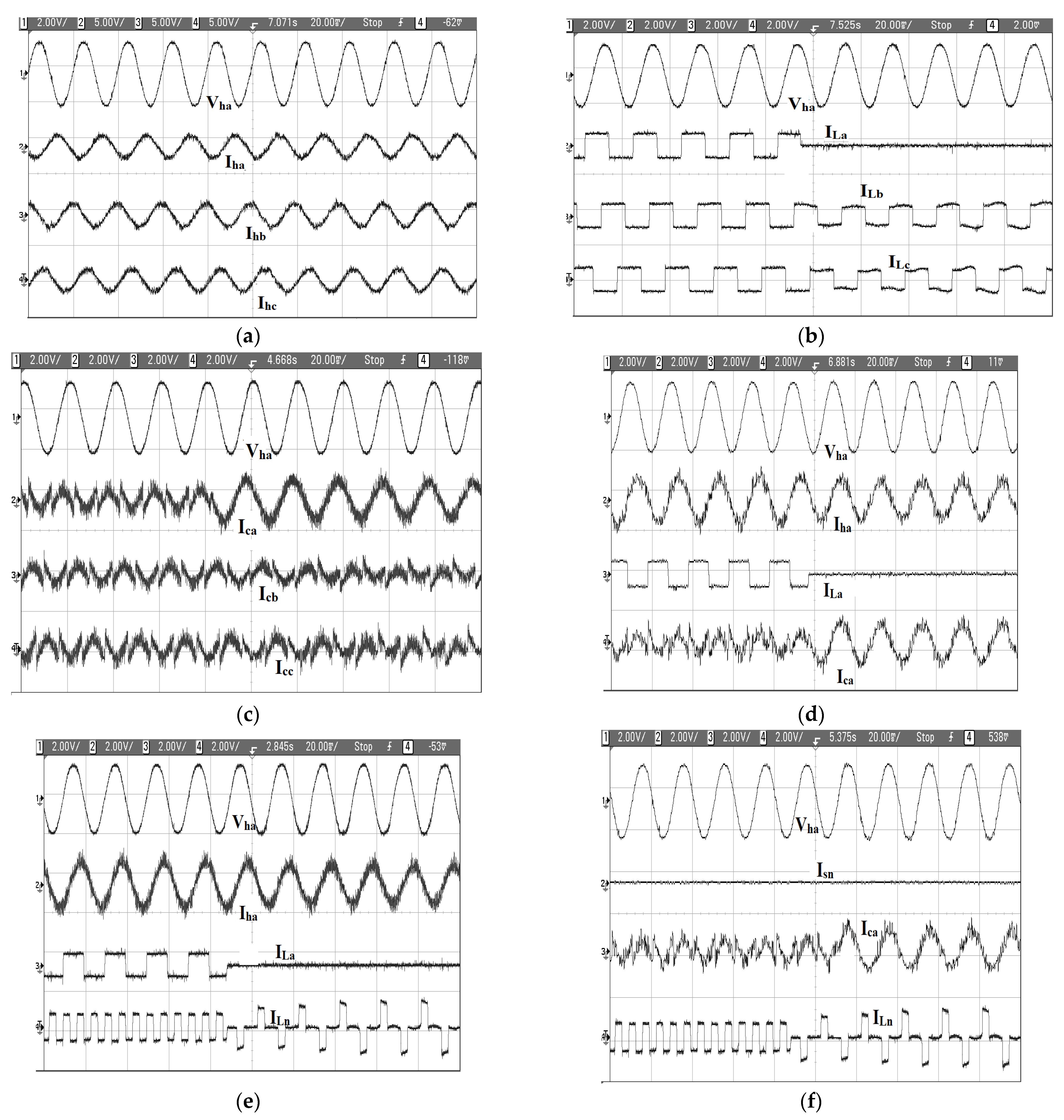
8. Hardware Results
Figure 14a–f shows the experimental results of the proposed control algorithm as validated in the laboratory setup dSpace 1104. Figure 14a shows the source voltage and the source currents in each phase under normal operation. Figure 14b shows the waveforms under a disturbance. Phase a becomes disconnected whereas the other two phases are undisturbed. Figure 14c displays the compensating currents in each phase during the load disconnection. Figure 14d shows the source current, load current and compensating current during the load disconnection. The compensating current adjusts itself such that the source current does not become affected and it maintains the same waveform as under the normal operation. In Figure 14e, the source current, load current and the load neutral current is included. The changes in load neutral current during the load disconnection are shown. Figure 14f displays the source neutral current, compensating current and the load neutral current along with the voltage waveform. It is seen that the source neutral current is maintained zero even when the load neutral current becomes disturbed, during the load disconnection.
9. Conclusions
The study suggests the Leaky LMS algorithm as the controller for a standalone wind energy unit. LMS algorithm works on the online modification of weight. It works on finding the filter coefficients such that the least mean square value of the error signal is produced, which avoids the use of a filter to squeeze out the harmonics. This makes the system simpler and economical. An adaptive algorithm that is generally used in signal processing is applied in power system applications and the process is further simplified by using optimization techniques. That makes the proposed method very unique. Normalized LMS algorithm suffers from drift problem. The leaky factor helps to avoid the drift problem of the normal LMS algorithm and a convergence factor decides the rate of convergence and stability. The selection of these factors is very important as the efficiency of the system depends on these parameters. The proposed algorithm selects the parameters by adopting optimization techniques. The optimization has made the process of controller tuning very easy, which otherwise was carried out by the trial-and-error method. On comparing the results obtained by different optimization techniques, it is found that the Antlion algorithm works most effectively with this system. The controller efficiency is tested for loads that are linear and nonlinear and for varying wind speeds. It is found that the controller is very efficient in maintaining the system parameters under normal and faulty conditions. An unbalance was created and the variation in system parameters during the period of unbalance and after reconnecting the same are studied. The control algorithm is tested for a change in wind speed also. The results show that the controller with LLMS in association with the Antlion Optimization algorithm is very efficient and quick in maintaining the stability of the system under normal operation when there is a fault, and even when there is a change in wind speed. the Total Harmonic Distortion in source voltage and source current are very well under the limits specified by the IEEE standards under all these conditions. The simulated results are validated by doing the testing in a laboratory set up by using dSpace 1104. The results verify the efficiency of the proposed controller algorithm.
Author Contributions
Conceptualization, A.K. and R.V.; methodology, A.K. and N.R.K.; software, R.V. and S.R.S.; validation, A.K., R.V., N.R.K. and S.R.S.; formal analysis, A.K.; investigation, R.V.; resources, N.R.K. and S.R.S.; data curation, A.K.; writing—original draft preparation, A.K. and N.R.K.; writing—review and editing, R.V. and S.R.S.; visualization, A.K.; supervision, R.V. and N.R.K.; project administration, R.V. and S.R.S.; funding acquisition, R.V. and S.R.S. All authors have read and agreed to the published version of the manuscript.
Funding
This research work was funded by WOOSONG UNIVERSITY’s Academic Research Funding—2021.
Institutional Review Board Statement
Not applicable.
Informed Consent Statement
Not applicable.
Data Availability Statement
Not applicable.
Conflicts of Interest
The authors declare no conflict of interest.
References
- Boldia, I. Variable Speed Generator: The Electrical Generator Handbook; Taylor & Francis: New York, NY, USA, 2006. [Google Scholar]
- IEEE Std. IEEE Recommended Practices and Requirement for Harmonic Control on Electric Power System; IEEE Standards Association: Piscataway, NJ, USA, 1993; p. 141. [Google Scholar]
- Sergio, P.; Diniz, R. The least-mean-square (LMS) algorithm. In Part of The Springer International Series in Engineering and Computer Science Book Series; Springer: Berlin/Heidelberg, Germany, 2020; Volume 399. [Google Scholar]
- Bismor, D.; Czyz, K.; Ogonowski, Z. Review and comparison of variable step-size LMS algorithms. Int. J. Acoust. Vib. 2015, 21, 24–39. [Google Scholar] [CrossRef]
- Singh, B.; Rajagopal, V. A neural-network-based integrated electronic load controller for isolated asynchronous generators in small hydro generation. IEEE Trans. Ind. Electron. 2011, 58, 4264–4274. [Google Scholar] [CrossRef]
- Kamenetsky, M.; Widrow, B. A Variable Leaky LMS Adaptive Algorithm; IEEE: Piscataway, NJ, USA, 2014; pp. 125–128. [Google Scholar]
- Nayar, P.; Singh, B.; Mishra, S.; Niwas, R. A New Control Algorithm for Power Quality Improvement in a Stand-alone Synchronous Reluctance Generator with Energy Storage. Electr. Power Compon. Syst. 2016, 44, 2198–2211. [Google Scholar] [CrossRef]
- Mustafa, R.; Muad, A.M.; Jelani, S.H. A Nd Ahmad Nur Alifa Abdul Razap. Multiple Iteration of Weight Updates for Least Mean Square Adaptive Filter in Active Noise Control Application. In Proceedings of the MATEC Web of Conferences, Elazığ, Turkey, 12–14 May 2016. [Google Scholar] [CrossRef]
- Ram, M.R.; Madhav, K.V.; Hari, K.E.; Reddy, K.N.; Reddy, K.A. A Novel Approach for Motion Artifact Reduction in PPG Signals Based on AS-LMS Adaptive Filter. IEEE Trans. Instrum. Meas. 2012, 5, 1445–1457. [Google Scholar] [CrossRef]
- Gwadabe, T.R.; Salman, M.S.; Abuhilal, H. A Modified Leaky-LMS Algorithm. Int. J. Comput. Electr. Eng. 2014, 6, 222–225. [Google Scholar] [CrossRef] [Green Version]
- Chawda, G.S.; Shaik, A.G.; Mahela, O.P.; Padmanaban, S. Comprehensive Review of Distributed FACTS Control Algorithms for Power Quality Enhancement in Utility Grid with Renewable Energy Penetration. IEEE Power Energy Soc. 2020, 8, 107614–107634. [Google Scholar] [CrossRef]
- Bhattacharya, A.; Chakraborty, C. Predictive and adaptive ANN (adaline) based harmonic compensation for shunt active power filter. In Proceedings of the IEEE Region 10 and the Third international Conference on Industrial and Information Systems, Indian Institute of Technology, Kharagpur, India, 8–10 December 2008. [Google Scholar]
- Singh, B.; Solankib, J. An Implementation of an Adaptive Control Algorithm for a Three-Phase Shunt Active Filter. IEEE Trans. Ind. Electron. 2009, 56, 2811–2820. [Google Scholar] [CrossRef]
- Singh, B.; Arya, S.R.; Chandra, A.; Al-Haddad, K. Implementation of Adaptive Filter in Distribution Static Compensator. IEEE Trans. Ind. Appl. 2014, 50, 3026–3036. [Google Scholar] [CrossRef]
- Garanayak, P.; Panda, G. Harmonic Elimination and Reactive Power Compensation with a Novel Control Algorithm based Active Power Filter. J. Power Electron. 2015, 15, 1619–1627. [Google Scholar] [CrossRef]
- Elmetwaly, A.H.; Eldesouky, A.A.; Sallam, A.A. An Adaptive D-FACTS for Power Quality Enhancement in an Isolated Microgrid. IEEE Access 2020, 8, 57923–57942. [Google Scholar] [CrossRef]
- Bravo-Rodríguez, J.C.; Torres, F.J.; Borrás, M.D. Hybrid Machine Learning Models for Classifying Power Quality Disturbances: A Comparative Study. Energies 2020, 13, 2761. [Google Scholar] [CrossRef]
- García-Sánchez, T.; Mishra, A.K.; Hurtado-Pérez, E.; Puché-Panadero, R.; Bravo-Rodríguez, A.-F.-G.; Francisco, J.T.; Borrás, M.D. A Controller for Optimum Electrical Power Extraction from a Small Grid-Interconnected Wind Turbine. Energies 2020, 13, 5809. [Google Scholar] [CrossRef]
- Meegahapola, L.; Sguarezi, A.; Bryant, J.S.; Gu, M.; Conde, D.E.R.; Cunha, R.B.A. Power System Stability with Power-Electronic Converter Interfaced Renewable Power Generation: Present Issues and Future Trends. Energies 2020, 13, 3441. [Google Scholar] [CrossRef]
- Ghaffarzadeh, H.; Mehrizi-Sani, A. Review of Control Techniques for Wind Energy Systems. Energies 2020, 13, 6666. [Google Scholar] [CrossRef]
- Sawant, M.; Thakare, S.; Rao, A.P.; Feijóo-Lorenzo, A.E.; Bokde, N.D. A Review on State-of-the-Art Reviews in Wind-Turbine- and Wind-Farm-Related Topics. Energies 2020, 13, 2041. [Google Scholar]
- Mladenov, V.; Chobanov, V.; Georgiev, A. Impact of Renewable Energy Sources on Power System Flexibility Requirements. Energies 2021, 14, 2813. [Google Scholar] [CrossRef]
- Gajewski, P.; Pieńkowski, K. Control of the Hybrid Renewable Energy System with Wind Turbine, Photovoltaic Panels and Battery Energy Storage. Energies 2021, 14, 1595. [Google Scholar] [CrossRef]
- Allani, M.Y.; Riahi, J.; Vergura, S.; Mami, A. FPGA-Based Controller for a Hybrid Grid-Connected PV/Wind/Battery Power System with AC Load. Energies 2021, 14, 2108. [Google Scholar] [CrossRef]
- Kumar, K.; Vanukuru, P.B. Development of control techniques for SAPF for power quality enhancement. J. Adv. Res. Dyn. Control. Syst. 2018, 10, 1900–1907. [Google Scholar]
- Keerthi, N.; Pandian, A. Study on the control techniques for the SAPFs: A comprehensive analysis. Int. J. Emerg. Trends Eng. Res. 2019, 7, 628–633. [Google Scholar]
- Venkateswarlu, M.; Pakkiraiah, B. Power quality improvement of AC distribution system using 3 phase PV integrated UPQC with advanced control strategy. Int. J. Eng. Adv. Technol. 2019, 8, 819–827. [Google Scholar]
- Swapna, S.P.; Rajasekhar, G.G.; Vijay, M.T.; Sai, C.M. Power quality and custom power improvement using UPQC. Int. J. Eng. Technol. UAE 2018, 7, 41–43. [Google Scholar] [CrossRef] [Green Version]
- Guru, P.S.; Srikanth, K.S.; Rajanna, B.V. Advanced active power filter performance for grid integrated hybrid renewable power generation systems. Indones. J. Electr. Eng. Comput. Sci. 2018, 11, 60–73. [Google Scholar]
- Praveenkumar, B.; Srikanth, K.S.; Kiran, K.M.; Raja, S.G.G. ANN control based variable speed PMSG-based wind energy conversion system. Int. J. Eng. Technol. UAE 2018, 7, 526–531. [Google Scholar] [CrossRef] [Green Version]
- Bodha, V.R.; Srujana, A.; Kuthuri, N.R. Predictive back-to-back SCHVC for renewable wind power system for scrutinizing quality and reliability. Energy Sources Part A Recovery Util. Environ. Eff. 2019, 41, 3058–3075. [Google Scholar] [CrossRef]
- Sridevi, J.; Rani, V.U.; Rao, B.L. Integration of renewable dgs to radial distribution system for loss reduction and voltage profile improvement. In Proceedings of the IEEE International Conference on Electrical, Control and Instrumentation Engineering, ICACIE 2019, Kuala Lumpur, Malaysia, 25 November 2019. [Google Scholar]
- Sharath, B.V.; Burthi, L.R. A new STATCOM based reactive power management in grid connected DFIG based wind farm. Int. J. Innov. Technol. Explor. Eng. 2019, 8, 293–299. [Google Scholar]
- Bodha, V.R.; Kuthuri, N.R.; Srujana, A. Stabilization of the alternative current in wind based power plant using multi order harmonic remover based on synthesized multilayer power converter. Int. J. Innov. Technol. Explor. Eng. 2019, 8, 1935–1944. [Google Scholar]
- Abas, N.; Dilshad, S.; Khalid, A.; Saleem, M.S. Nasrullah Khan Power Quality Improvement Using Dynamic Voltage Restorer Filter. IEEE Access 2020, 8, 164325–164339. [Google Scholar] [CrossRef]
- Zhang, X.; Yan, Z. Energy Quality: A Definition. IEEE Open Access J. Power Energy 2020, 7, 430–440. [Google Scholar] [CrossRef]
- Mirjalili, S. The Ant Lion Optimizer. Adv. Eng. Softw. 2015, 83, 80–98. [Google Scholar] [CrossRef]
- de Almeida, B.S.G.; Leite, V.C. Particle swarm optimization: A powerful technique for solving engineering problems. In Swarm Intelligence-Recent Advances, New Perspectives and Applications; Intech Open: London, UK, 2019. [Google Scholar]
- Mirjalili, S. The Whale Optimization Algorithm. Adv. Eng. Softw. 2016, 95, 51–67. [Google Scholar] [CrossRef]
- Bastos, A.F.; Santoso, S. Optimization Techniques for Mining Power Quality Data and Processing Unbalanced Datasets in Machine Learning Applications. Energies 2021, 14, 463. [Google Scholar] [CrossRef]
- Vadi, S.; Padmanaban, S.; Bayindir, R.; Blaabjerg, F.; Mihet-Popa, L. A Review on Optimization and Control Methods Used to Provide Transient Stability in Microgrids. Energies 2019, 12, 3582. [Google Scholar] [CrossRef] [Green Version]
- Jumani, T.A.; Mustafa, M.W.; Hamadneh, N.N.; Atawneh, S.H.; Rasid, M.M.; Mirjat, N.H.; Bhayo, M.A.; Khan, I. Computational Intelligence-Based Optimization Methods for Power Quality and Dynamic Response Enhancement of ac Microgrids. Energies 2020, 3, 4063. [Google Scholar] [CrossRef]
Figure 1.
(a) Turbine output power Vs turbine speed when the pitch angle is zero-degree. (b) Turbine output power Vs turbine speed when the pitch angle is 7 degrees.
Figure 1.
(a) Turbine output power Vs turbine speed when the pitch angle is zero-degree. (b) Turbine output power Vs turbine speed when the pitch angle is 7 degrees.

Figure 2.
Schematic diagram of the Wind Power Harnessing Unit under study. Vha, Vhb and Vhc: Source voltages (harnessed voltages); Iha, Ihb, and Ihc: Source currents in phase a, phase b and phase c respectively; ILa, ILb, ILc: Load currents in phase a, phase b and phase c respectively; Ica, Icb, Icc: Compensating currents, Ic: Current through the excitation capacitor, Ib: Battery current; Vb: Battery voltage, Rin: Internal resistance of the battery, Cb: Battery Capacitance, Rb: Resistance of the capacitor, Lf: Filtering inductor.

Figure 3.
Control Algorithm.

Figure 4.
(a) Trajectory of frequency PI gain; (b) Trajectory of AC PI gain; (c) Convergence curve using Antlion algorithm(ALO).
Figure 4.
(a) Trajectory of frequency PI gain; (b) Trajectory of AC PI gain; (c) Convergence curve using Antlion algorithm(ALO).

Figure 5.
(a) Trajectory of frequency PI gain; (b) Trajectory of AC PI gain; (c) Convergence curve using Particle Swam Optimization (PSO).
Figure 5.
(a) Trajectory of frequency PI gain; (b) Trajectory of AC PI gain; (c) Convergence curve using Particle Swam Optimization (PSO).

Figure 6.
(a) Trajectory of frequency PI gain; (b) Trajectory of AC PI gain; (c) Convergence curve using Whale Optimization Algorithm (WOA).
Figure 6.
(a) Trajectory of frequency PI gain; (b) Trajectory of AC PI gain; (c) Convergence curve using Whale Optimization Algorithm (WOA).

Figure 7.
(a) Trajectory step size and leaky factor using ALO, (b) Trajectory step size and leaky factor using PSO and (c) Trajectory step size and leaky factor using WOA algorithm.
Figure 7.
(a) Trajectory step size and leaky factor using ALO, (b) Trajectory step size and leaky factor using PSO and (c) Trajectory step size and leaky factor using WOA algorithm.

Figure 8.
Performance of the Wind power unit with linear load at constant wind speed.

Figure 9.
Performance of the Wind power unit with nonlinear load at constant wind speed.

Figure 10.
Performance of the Wind power unit with nonlinear load when the wind speed changes from 11 m/s to 13 m/s.
Figure 10.
Performance of the Wind power unit with nonlinear load when the wind speed changes from 11 m/s to 13 m/s.

Figure 11.
Performance of the Wind power unit with the nonlinear load when the wind speed changes from 11 m/s to 13 m/s.
Figure 11.
Performance of the Wind power unit with the nonlinear load when the wind speed changes from 11 m/s to 13 m/s.

Figure 12.
(a) Total Harmonic Distortion (THD) in source voltage (b) THD in source current w.r.t frequency.
Figure 12.
(a) Total Harmonic Distortion (THD) in source voltage (b) THD in source current w.r.t frequency.

Figure 13.
(a) THD in source voltage (b) THD in source current plotted against the harmonics.

Figure 14.
(a) source voltage and source currents in 3 phases under normal conditions (b) Source voltage and load currents in 3 phases when phase ‘a’ is disconnected (c) Source voltage and compensating currents in 3 phases when phase ‘a’ is disconnected (d) Source voltage, source current, load current and compensating current when phase ‘a’ is disconnected (e) Source voltage, source current, load current and load neutral current when phase ‘a’ is disconnected (f) Source voltage, source neutral current, compensating current and load neutral current when phase ‘a’ is disconnected.


Table 1.
P and I gain values, step-size and the Leaky factor as obtained from various optimization techniques.
Table 1.
P and I gain values, step-size and the Leaky factor as obtained from various optimization techniques.
| Frequency PI Gains | AC PI Gains | Convergence of Cost Function | Step-Size μ | Leaky Factor β | Suitability of the Optimization Algorithm | |||
|---|---|---|---|---|---|---|---|---|
| Algorithm | Kp | Ki | Kp | Ki | ||||
| ALO | 4.3173 | 2.7903 | 0.28459 | 1.0907 | 8272.9343 | 0.24979 | 0.36096 | The Best suited for the system |
| PSO | 1.1388 | −0.8312 | 2.8596 | 0.64372 | 1753.6756 | 1.7625 | −0.8053 | Not suitable |
| WOA | 1.0055 | 0 | 0 | 0.7579 | 7757.8788 | 0.18243 | 0.1671 | Not suitable |
Publisher’s Note: MDPI stays neutral with regard to jurisdictional claims in published maps and institutional affiliations. |
© 2021 by the authors. Licensee MDPI, Basel, Switzerland. This article is an open access article distributed under the terms and conditions of the Creative Commons Attribution (CC BY) license (https://creativecommons.org/licenses/by/4.0/).
Share and Cite
MDPI and ACS Style
Kodakkal, A.; Veramalla, R.; Kuthuri, N.R.; Salkuti, S.R. An ALO Optimized Adaline Based Controller for an Isolated Wind Power Harnessing Unit. Designs 2021, 5, 65. https://0-doi-org.brum.beds.ac.uk/10.3390/designs5040065
AMA Style
Kodakkal A, Veramalla R, Kuthuri NR, Salkuti SR. An ALO Optimized Adaline Based Controller for an Isolated Wind Power Harnessing Unit. Designs. 2021; 5(4):65. https://0-doi-org.brum.beds.ac.uk/10.3390/designs5040065
Chicago/Turabian StyleKodakkal, Amritha, Rajagopal Veramalla, Narasimha Raju Kuthuri, and Surender Reddy Salkuti. 2021. "An ALO Optimized Adaline Based Controller for an Isolated Wind Power Harnessing Unit" Designs 5, no. 4: 65. https://0-doi-org.brum.beds.ac.uk/10.3390/designs5040065