Impact of Pavement Surface Condition on Roadway Departure Crash Risk in Iowa


1
Civil, Construction and Environmental Engineering/Center for Transportation Research and Education, Iowa State University, Ames, IA 50010, USA
2
Industrial and Manufacturing Systems Engineering, Iowa State University, Ames, IA 50011, USA
*
Author to whom correspondence should be addressed.
Infrastructures 2018, 3(2), 14; https://0-doi-org.brum.beds.ac.uk/10.3390/infrastructures3020014
Submission received: 19 May 2018
/
Revised: 10 June 2018
/
Accepted: 12 June 2018
/
Published: 13 June 2018
(This article belongs to the Special Issue Sustainable Transportation Infrastructures)
Abstract
:Safety performance is a crucial component of highway network performance evaluation. Besides their devastating impact on roadway users, traffic crashes lead to substantial economic losses on both personal and societal levels. Due to the complexity of crash events and the unique conditions in each country and state, empirical local calibration for the correlation between attributes of interest and the safety performance is always recommended. Limited studies have established a procedure to analyze the impact of pavement condition on traffic safety in a risk analysis scheme. This study presents a thorough analysis of some roadway departure crashes which occurred in Iowa between 2006 and 2016. All crash records were mapped onto one-mile segments with known traffic volume (i.e., AADT), posted speed limits (SL), skid numbers (SN), ride qualities (IRI), and rut depths (RD) in a geographic information system (GIS) database. The crash records were correlated to the pavement surface condition (i.e., SN, IRI, and RD) using negative binomial regression models. Moreover, a novel risk analysis framework is introduced to perform crash risk assessment and evaluate the possible consequences for a given combination of events. The analysis shows a significant impact of pavement skid resistance on roadway-departure crashes under all accident conditions and severities. Risk analysis will facilitate coordination between the pavement management system and safety management system in the future, which will help with optimizing the overall highway network performance.
1. Introduction
Safety performance is a crucial component of a highway network performance evaluation. Besides their devastating impact on roadway users, traffic crashes lead to substantial economic losses on both personal and societal levels [1]. Due to the complexity of a traffic crash event, it is a challenging task to identify all the contributing factors, and even more challenging to quantify their level of impact on crash rates [2,3]. Some of these factors include driver behavior and human factors, traffic conditions, road geometrics, pavement surface condition, and traffic speed. Pavement surface condition can include multiple variables; however, the possible key contributors to traffic safety are pavement friction (i.e., skid resistance), roughness (i.e., ride quality), and rutting [4,5]. Maintaining pavement surface conditions at acceptable levels is part of pavement management activities; accordingly, previous studies have proposed incorporating the impact of pavement surface condition on traffic safety into pavement management systems (PMSs) [2,6].
Several studies have investigated the relationship between pavement surface friction and crash risk, and could quantify significant correlations between them. However, these correlations can be delusive and challenging to derive due to the highly varied and uncontrolled conditions during a crash event [7,8]. One of the most extensive efforts in this research area is the National Corporative Research Program (NCHRP) project 01-43 “Guide for Pavement Friction”. The project report was published in 2010 [9]. In the report, quantitative correlations between wet crash rates and pavement friction values could be found in more than 15 studies in the literature. The study focused on describing and illustrating the importance of friction in highway safety, as well as the principles of pavement friction characterization. Furthermore, the study presented valuable information on (a) the management of friction on existing highway pavements, and (b) the design of new highway surfaces with adequate friction. This information focuses on techniques for monitoring friction and crashes, and determining the need for remedial action. However, two components, friction and safety management, are still disconnected and not synchronized efficiently.
Pavement friction develops between the tire and the pavement due to the hysteresis and adhesion mechanisms at the tire-pavement interface [9,10]. The two mechanisms, strongly depend on the contact surface area between the tire and the pavement surface, which in turn depend on several factors including pavement texture, surface contamination (e.g., wet, dry, dusty), and tire rubber stiffness [11]. In 2009, Mayora and Piña [12] coupled crash data and skid resistance data, measured with a sideway-force coefficient routine investigation machine (SCRIM), to investigate the effect of pavement condition on safety, and to assess the effects of improving pavement friction on safety. It was found that under wet and dry conditions, crash rates decreased as skid resistance increased. To develop causal relationship between pavement condition indices and severity level of crashes occurring on two-lane horizontal curves in Texas, Buddhavarapu et al. [13] integrated crash and pavement surface condition databases. From the study, it was found that longitudinal skid measurements barely correlated with the injury severity of crashes occurring on curved portions of road. Interestingly, it was also reported that smoother sections were more vulnerable to severe crashes. Musey and Park [14] have conducted a comprehensive review of crash data to correlate pavement skid numbers and roadway curvature degree to crash rates and severity. It was found that greater injuries occurred on curves with higher degrees of curvature and lower skid numbers. In the study [14], the crash rates, normalized using the average annual daily traffic (AADT), showed a bell-curve when plotted against skid number. Therefore, the crash rates start increasing as the skid number increases, and peak at around 40, then start to decrease as skid number increases. The authors attributed this behavior to the increasing AADT values at sections with low skid numbers, which in turn had an inverse relation to the crash rates in their study.
Pavement friction enhancements and treatments were included in the United States Department of Transportation Federal Highway Administration (FHWA) Pooled Fund Study “Evaluation of Low-Cost Safety Improvements” (ELCSI–PFS). The study was established to conduct research on the effectiveness of the safety improvements identified by the (NCHRP) Report 500 guides [15,16]. In volumes 6 and 7 of the NCHRP report, strategies 15.1 A7 and 15.2 A7 included the use of skid-resistant pavements as a key strategy for reducing run-off-road crashes and crashes on horizontal curves [17]. In a similar manner, the FHWA “Low-Cost Treatments for Horizontal Curve Safety Guide” recommends “skid-resistive pavement surface treatments” as a low-cost treatment for reducing crashes at horizontal curves [17,18]. According to the FHWA, high friction surface treatments (HFSTs) are a highly cost-effective countermeasure that can be applied for one or more of the following situations: sharp curves, inadequate cross-slope design, wet conditions, polished roadway surfaces, and driving speeds in excess of the curve advisory speed [19].
More recently, the Virginia Department of Transportation (DOT) adopted some of the concepts developed by a research team at Virginia Tech Transportation Institute to modify their current safety performance functions [20,21,22,23]. In the reported studies, the research team has utilized a low-cost, continuous friction-measuring device, the Grip Tester, to acquire friction measurements for a single district. The friction data was then coupled with crash records to quantify the impact of friction measurements on crash rates. The data was used to contrast the effect of two friction treatments, i.e., conventional asphalt overlay and HFSTs, on network level crash rates. The result suggests significant crash reductions with comprehensive economic savings of $100 million or more when applying the HFSTs to a single district. Moreover, Geedipally et al. [24] conducted a study to develop a crash modification factor (CMF) for skid number for all crashes, wet-weather crashes, run-off-the-road crashes, and wet-weather run-off-the-road crashes. The study evaluation was conducted based on a horizontal curve database from a southern state in the United States. The findings confirmed that skid number was a significant variable, in addition to traditional variables such as traffic volume, curve radius, and cross-sectional width.
Pavement rutting is suspected of affecting traffic safety by forming a water film or a stagnant pool between the pavement surface and the tire. This water film will induce hydroplaning and cause loss of control, which can lead to a crash event [25,26,27]. Start et al. [25] presented a study to quantify the effects of pavement rutting on accident rates. The researchers analyzed rut depth, traffic volumes, and accident records maintained by the Wisconsin DOT for undivided rural highways. Accidents were classified to rut-related crashes if the prevailing conditions could be potentially associated with the occurrence of hydroplaning. The results indicated that rut-related accident rates began to increase at a significantly greater rate as rut depths exceeded 7.6 mm. More analytically-intensive approaches have been proposed to evaluate the impact of rutting on traffic safety [27,28,29]. Ong and Fwa [26] presented a paper that adopts an elaborate theoretical approach to simulate hydroplaning and the reduction of wet-pavement skid resistance as a function of wheel sliding speed. The findings conformed to the well-known experimentally derived NASA hydroplaning-speed equation. Despite the significant findings from simulations and analytical approaches, analyses of crash records and the PMS database do not always show strong correlations between hydroplaning and crash rates [4,30].
Researchers have also investigated the impact of ride quality on traffic safety [13,30,31]. Chan et al. [30] utilized the Tennessee PMS and the accident history database to investigate the relationship between accident frequency and pavement surface condition. The pavement condition metrics included rut depth (RD), ride quality expressed in terms of the international roughness index (IRI), and present serviceability index (PSI). Poisson regression was used to model the probability of an accident given the pavement and traffic condition. The models showed that for all accident types, higher IRI values will significantly increase the risk of an accident. In contrast, Buddhavarapu et al. [13] reported that smoother roads can lead to higher accident severity. Other studies have reported similar findings [2,32]. Tighe et al. [2] suggested that rougher roads can possibly lead to a higher level of vigilance, which can reduce the risk of accidents.
Despite the available literature investigating the impact of pavement condition—including surface skid resistance—on crash rates, each country and state has unique conditions, including traffic characteristics, drivers’ behavior, and weather conditions. Therefore, due to the complexity of crash events, empirical local calibration for correlations between attributes of interest and safety performance are always recommended. Moreover, there are few efforts, if any, to describe these safety correlations and functions in a risk analysis scheme. This study presents an effort to integrate elements of the pavement surface condition records, acquired from the PMS database, with the roadway departure crash records in the state of Iowa in the United States. Risk analysis is a combination of uncertainty and consequences. The consequences of traffic accidents can include casualties, vehicle damage, monetary costs, and even societal impacts. This paper focuses on establishing a framework for one part of the risk analysis, estimating the probability of crashes. Risk analysis will facilitate the integration between the PMS and safety management system in an effort to optimize the overall highway network performance.
2. Data Sources
2.1. Pavement Condition Data
The Iowa PMS database includes records for various pavement conditions and traffic information in a geographic information system (GIS) database, including traffic volume (AADT), speed limit (SL), skid resistance expressed in skid number (SN), ride quality expressed in IRI, and rut depth (RD). All the mentioned variables, besides the AADT, which is a major contributor to the model, were considered as possible explanatory variables of possible impact. The study included records for one mile segments acquired between 2006 and 2016. Each record had a unique combination of identifiers, including the acquisition year and the mile ID. The Iowa DOT collects friction measurements at the network level on a 2-year cycle for interstate segments, a 3–5 year cycle for primary non-interstate segments depending on the AADT, and annual monitoring for segments with low SNs. Other pavement condition data, including IRI and RD, are collected annually on the interstate, and biannually for primary non-interstate segments.
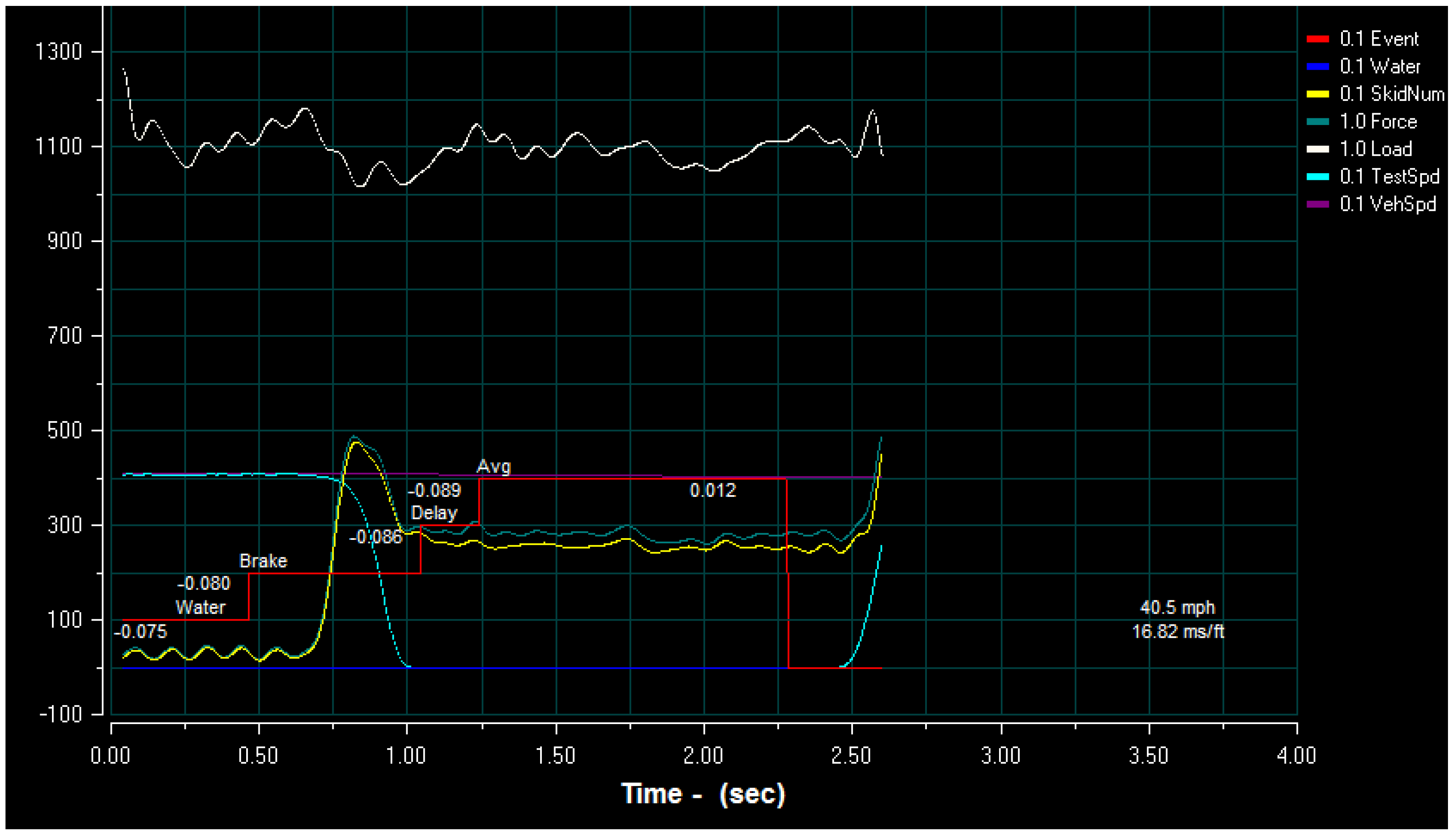
Pavement friction measurements are collected using a locked wheel skid trailer, and following the ASTM standard E274 [33]. The test device records the tractive force, defined as the horizontal force applied to the test tire at the tire-pavement contact patch, and the dynamic vertical load on the test wheel. The ratio of tractive force to the vertical load multiplied by 100 defines the skid number at a given testing condition, including the test speed. During the test, the trailer wheels are locked after applying water to the test surface. Figure 1 presents a typical screenshot of the locked wheel test output. In the figure, it can be seen that the SN (the yellow line in the figure) fluctuates around zero, when the tire rotates over the pavement surface without sliding. Then, as the rolling speed decreases, and the sliding speed increases accordingly, the SN increases to reach a peak value before dropping back to a fully-locked SN, where the rolling speed reaches zero.
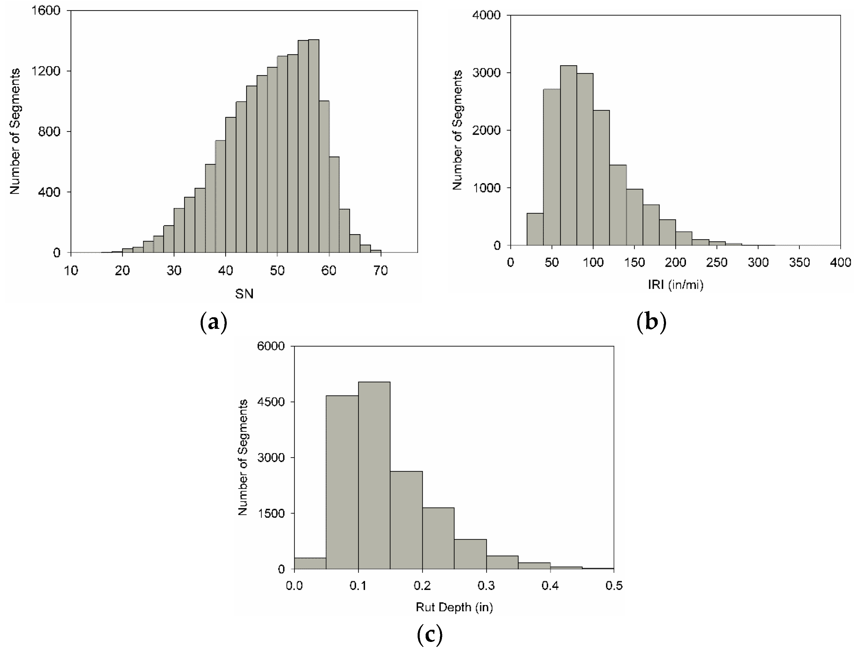
The IRI and RD were reported for the left and right wheel paths. The averages of the right and the left wheel paths were used to represent the segment IRI and RD values, which are used as explanatory variables in the study. The segments included in this study are one mile long. Only the segments with all pavement conditions, traffic volume, and speed limit records were included in the analysis, which eliminates segments with one or two missing pavement condition attributes. Figure 2a–c shows the histogram of SN, IRI, and RD values for the segments included in the study. Figure 2a shows that the SN distribution is slightly left-skewed, meaning that although the majority of the segments have relatively medium to high SNs, there are few segments with low SNs. Figure 2b,c shows that both IRI and RD values are right-skewed, indicating that more segments have lower IRI and RD values, indicating a good pavement condition.
2.2. Crash Records
Crash records for roadway departure crashes between 2006 and 2016 were acquired from the Iowa Traffic Safety Data Service (ITSDS). The records were linked with the condition data in a GIS database. Crash records that matched segments with condition data were merged to add crash attributes to the selected segments, which included 15,759 crash records. Crash records contained several attributes, including the severity of crash and the environmental surface condition (e.g., wet, dry, snow) during crash time. Figure 3a shows the percentage of crashes under each severity level for all crashes included in the study. The severity levels in the database were: (1) fatal crash, (2) crash with major injury, (3) crash with minor injury, (4) crash with possible/unknown injury, and (5) crash with property damage only. The environmental surface conditions found in the crash records are dry, wet, ice/frost, snow, slush, mud/dirt, standing water, sand, oil, and gravel. Due to the subjectivity in judging the surface conditions when it falls between ice/frost, snow, and slush, the three categories were combined together into adverse winter condition. The analysis included the three major environmental surface conditions: dry, wet, and adverse winter conditions. Figure 3b shows the distribution of crashes based on surface condition.
3. Methods
3.1. Crash Rate Models
Crash events are rare count events affected by multiple variables and conditions. The complexity of a crash event limits the ability of deriving a deterministic or quasi-deterministic model which can explain and predict a crash scenario and the sequence of events during the crash. As an alternative, researchers and practitioners have recommended using crash history data to establish the correlation between the expected number of crashes and the explanatory variables of interests [34]. Due to the discrete nature of count data, limited regression models are permissible to describe these correlations. A permissible regression model should allow for discrete and strictly positive observations. Amongst the permissible models are the Poisson and the Negative Binomial (NB) regression models. In Poisson regression, the fitted trend represents the mean number of events occurring within a given exposure period or extent. One limitation of the Poisson model is the assumption of equi-dispersion, where the expected number of events (Y) is equal to the variance given any set of explanatory variables. Alternatively, NB regression is a generalization of Poisson regression that allows for over-dispersed data, where the variance is equal to or greater than the expected value of the fitted model, which is a typical characteristic of crash count data [35].
In an NB regression model, the expected crash rate per unit exposure for a given road segment can be expressed as a function of the explanatory variables, as shown in Equation (1).
where is the expected crash rate on segment i, are the fitted regression coefficients, is the jth attribute of segment i, and n is the number of explanatory attributes included in the model. In addition to the fitted regression coefficients, a dispersion parameter is estimated and tested for significance. Typically, the exposure is expressed as the traffic volume (i.e., AADT) raised to a power multiplied by the segment length . In this study, all segments were 1 mile long, which drops the second term in Equation (1). Accordingly, Equation (1) can be simplified and expressed compactly in vector notation, as shown in Equation (2).
3.2. Risk Analysis
Although Equation (2) provides a good summary index that can be used as a comparison tool for the safety performance of a highway segment, it only represents the expected number of crashes. To perform a full scale analysis and to estimate the associated risks for a given road segment, a more elaborate analysis is required. Risk analysis can provide extra information about the distribution of severity levels, which gives an extra breadth into the analysis. To quantify the probability of having a specific number () of independent crashes, one can use the NB probability mass function (PMF) associated with the regression coefficients. Equation (3) is the PMF for observing crashes, given the total number of vehicles passing and the probability of crash for each vehicle passing:
Using a different parametrization, Equation (3) can be rewritten as a Gamma mixture of Poisson distributions, as shown in Equation (4). This parametrization only depends on the fitted NB regression coefficients, where and [36].
where is the gamma function and is the dispersion coefficient of the NB regression. Equation (4) estimates the probability of having a certain number of crashes regardless of the crash severity. To estimate impact of traffic crashes on the users and the agency, one can estimate the expected consequences of traffic crashes for a given segment. One common measure of risk is the probability of an event occurring multiplied by its consequences. Consequences can include the monetary value of losses due to a crash with a given severity, the societal impact, human injury, and travel delays. In this study, risk analysis will be limited to the distribution of severity level combinations.
Defining risk in a mathematical framework is necessary to generalize the computational process of risk assessment. The first element in the mathematical framework is the risk space (RS), in which all possible scenarios exist. The risk space can be divided into subspaces, namely risk surfaces (), where each surface represents the possible severity level combinations for crashes. A risk space is discrete and dense in the severity discrete space ,
where is the set of natural numbers, and the set of possible severities for the source of hazard , which is the possible severity levels for crash . In this study, the severity space reduces to because all crashes are independent and identically distributed for a given segment with the same possible severity levels , where . For no crash events, the risk surface reduces to the single event (i.e., no crash set; ).
Given that RS is a dense space, each point on the corresponds to one possible combination of severity levels:
where is the severity level of crash y and is the size of severity space . Equation (6) defines the risk surface as a tensor of rank and dimensionality . For example, for a given segment the risk surface corresponding to two crashes, , with 5 possible severity levels for each crash, is a second rank tensor, as shown in Equation (7).
The first element in the risk surface tensor shown in Equation (7) corresponds to the single scenario where the first crash occurs with severity level 1 (i.e., ), and the second with severity 1.
All risk surfaces can be projected into a probability subspace and a consequences subspace. The probability and consequences subspaces have the same size and dimensionality as the projected risk surface; therefore, the full probability and consequences spaces have the same size and dimensionality as the risk space. For each element in RS, there is a function that maps the severity combination into the consequences space, , where is an element of the consequence tensor. It should be mentioned that for y = 0, the consequences tensor collapses to a scaler of value zero, corresponding to zero consequences. Equation (8) defines the projection of the elements on the risk surface into the probability space.
where is the combination of severity levels for crashes. Given that the assumption that the severity level for each crash is independent of the segment condition and from the other crashes, Equation (8) can be rewritten as shown in Equation (9).
where is the probability of crash occurring with severity . The admissibility conditions for the risk space are defined in Equation (10). The admissibility conditions guarantee that the probability distribution for all possible scenarios in the risk space are a valid PMF. The first condition states that for a given number of crashes , the total probability of all possible severity combinations, elements of the severity space , should add to one. The second condition states that for a given risk space the total probability across all risk surfaces should add to one.
The probability distribution that a crash will occur at a severity level can be fitted using a parametric distributions. Alternatively, assuming independence of the severity level distribution from the segment condition, the simple empirical estimation defined in Equation (11) can be used to define the distribution.
where is the total number of crashes of severity , and is the total number of crashes.
To assess the impact of the explanatory variables on the crashes occurring under different environmental surface conditions, NB regression models can be derived for crashes that occurred on segments during a given environmental surface condition. Amongst the various environmental surface conditions in the crash records, the dry and wet conditions are the only conditions considered in the analysis. Crashes which occurred during the adverse winter conditions are far more complex, and the separate fitted models for such conditions can be misleading. To fit a conditional NB regression model, given the environmental surface condition (i.e., SC), only segments with crashes occurred under these conditions are included in the data set. Moreover, the NB distribution should be shifted, as shown in Equation (12), to exclude the segments that did not have crashes occur during the surface condition SC (i.e., ).
4. Results and Discussion
In this section, the numerical results from implementing the proposed methods in Section 3 are presented, along with the discussion. It should be noted that all the developed models serve as descriptive models rather than predictive ones. To construct predictive models for future uses, extensive data sets and carful revisions should be conducted to filter the data sets and carefully choose the proper models.
4.1. Visual Diagnostics
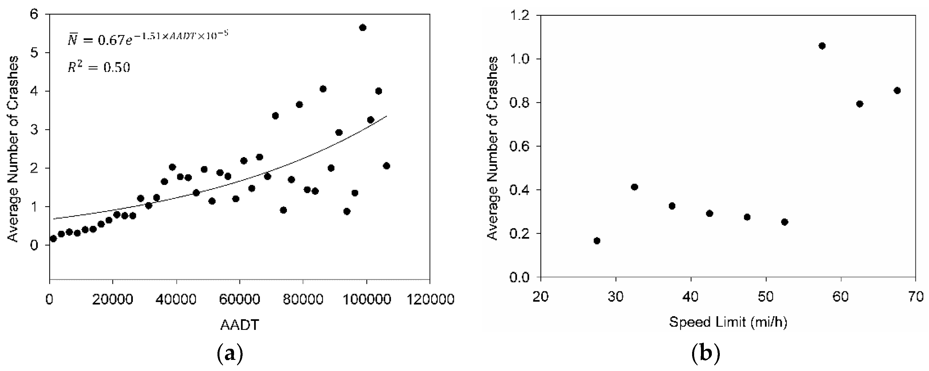
The first step in the analysis, i.e., before performing the regression analysis, is to diagnose the trends between the average number of crashes on each segment and the five explanatory variables, which included: AADT, SL, SN, IRI, and RD. To plot the empirical trend between AADT and the average number of crashes, the segments in the study were grouped based on AADT bins, which increased at 2500 increments. From Figure 4a, the average number of crashes for the segments within the bins increased as the AADT increased. Simple regression line shows that the correlation follows a power trend. The presented regression line is not statistically permissible due to the simple regression model assumptions in the NB model, however it is provided to facilitate the visual diagnostics. In Figure 4b, the speed limit (SL) ranged from 25 to 70 mi/h, with bin size 5 mi/h. From the figure, it can be seen that there is a jump in the average number of crashes after 55 mi/h. This can be an artifact due to the higher AADT on sections with SL > 55 mi/h.
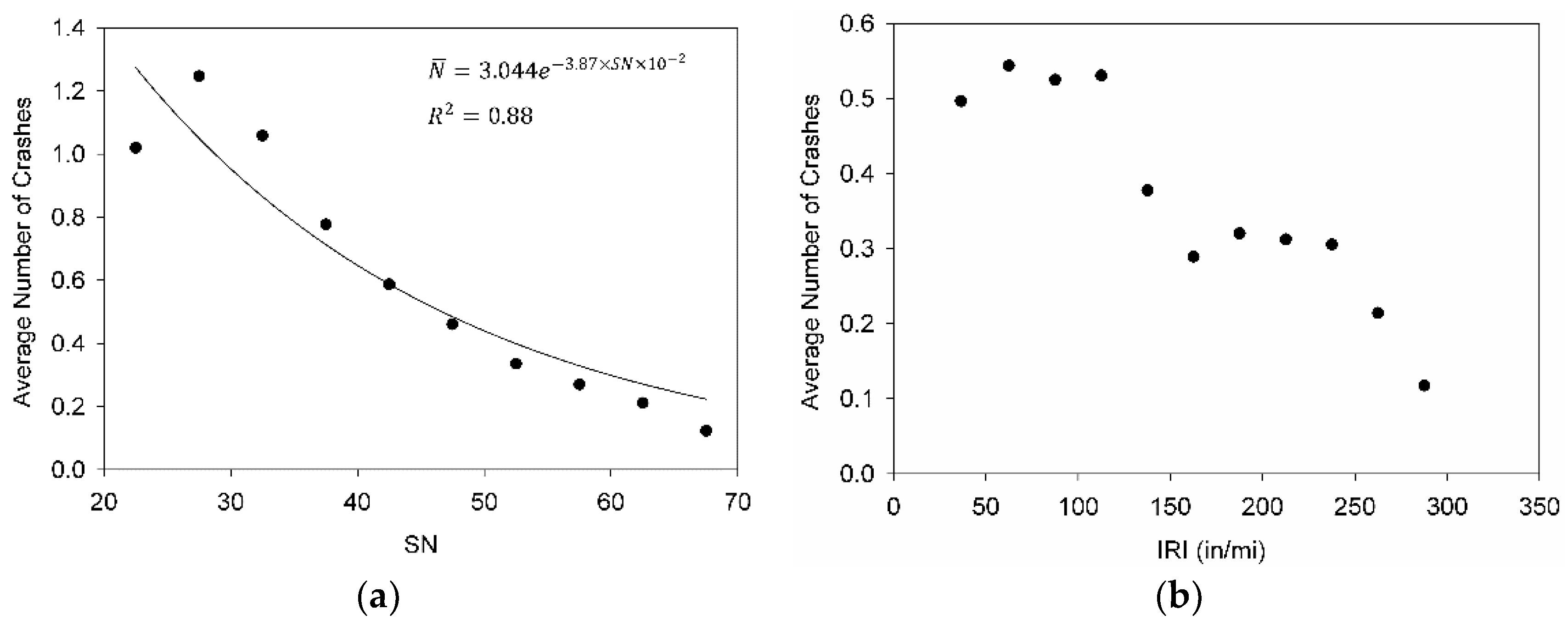
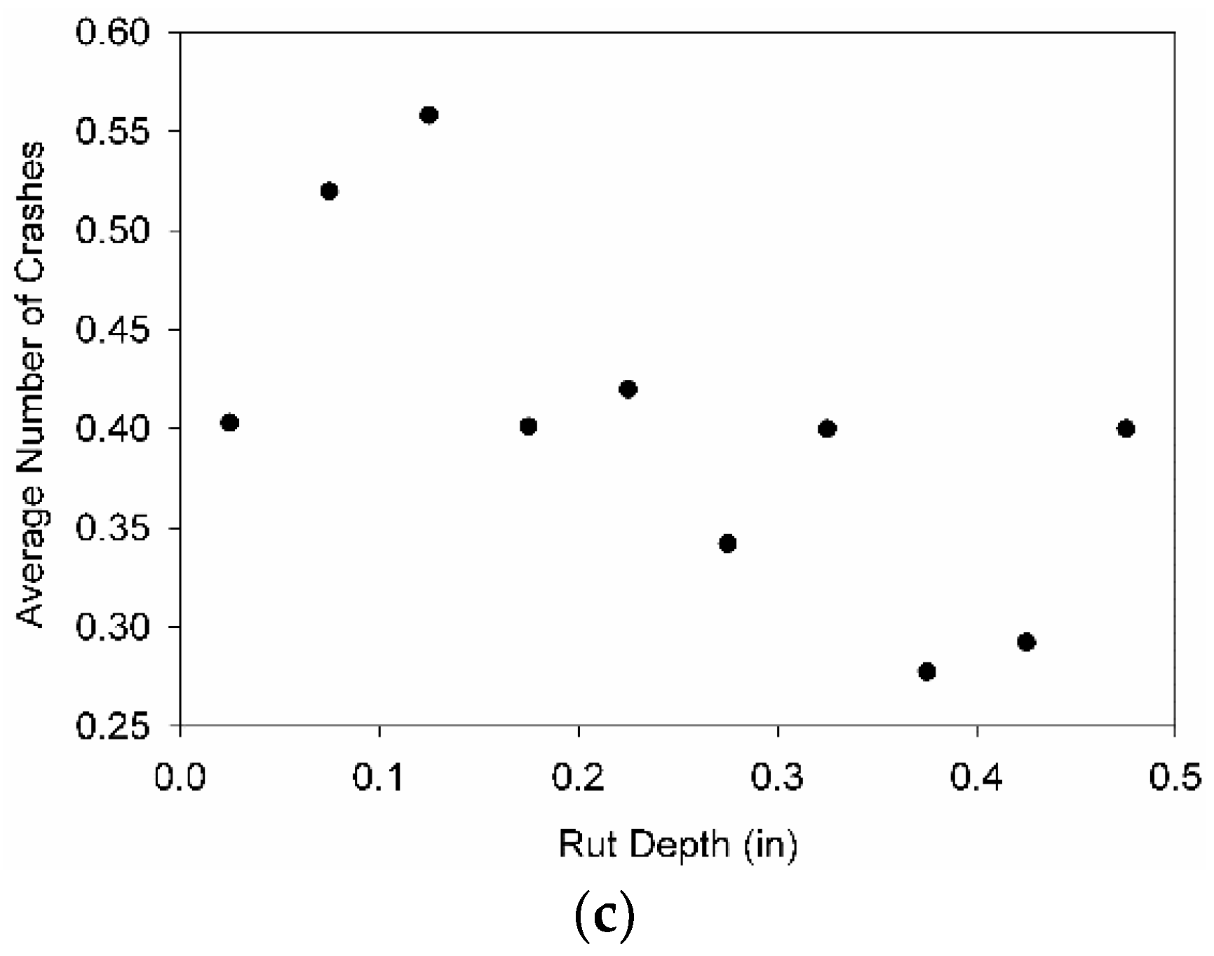
Figure 5a shows the trend between the average number of crashes and the SN for the corresponding segments. The SN values ranged between 20 and 70 with a bin size of 5. In Figure 5a, the average number of crashes follows a decaying trend as a function of the SN. Moreover, Figure 5b shows that generally, the average number of crashes decreased as the IRI value increased. Figure 5c does not reflect a clear trend between the average number of crashes and the RD. It should be mentioned that the trends shown in Figure 4 and Figure 5 do not necessarily reflect the type of correlation expected when performing the NB regression. These empirical trends do not incorporate the number of segments within each bin and the impact of other variables on the trend. For example, some sections with high AADT might have lower SN; therefore, the higher crash rate can be due to the high volume of traffic and not due to low SN. In contrast, NB regression can account for these interactions and the varying number of segments within explanatory variables bins.
4.2. Crash Rate Models
Table 1 summarizes the regression models fitted for various conditions in JMP Pro 12 [37]. All models were fitted using the five explanatory variables and the interaction between these variables and the posted speed limit. Moreover, a binary variable was introduced to capture the jump in the average number of crashes after 55 mi/h speed limit (Figure 4b). The explanatory variables were tested for significance using the Wald Chi-square test, where the null hypothesis is , for all j. Table 1 only includes the significant model terms, which have a p-value less than 0.05. For the three fitted models, the dispersion coefficient α was significantly greater than zero, indicating an over-dispersion in the data set, which requires a NB regression model. The dispersion coefficient is constant for all sections for each fitted model.
In Table 1, the general model was derived using the full crash record, including segments with no crashes and without distinction between severity levels and surface conditions. From the model, it can be noticed that in addition to the traffic volume (AADT), SN and IRI had a significant impact on the expected crash rate for all segments. The traffic volume (AADT) had a major impact on the expected crash rate; this can be attributed to the higher level of exposure, where the increased number of vehicles will increase the chance of a crash event occurring. Figure 6 shows that the expected crash rate dropped as the SN increases for various AADT, SL, and a fixed IRI = 90 in/mi. This reduction in expected crash rates is due to the reduction in probability of a skidding event. Moreover, Figure 6 shows that as the speed limit increases, the expected crash rate decayed at higher rate with increasing SN values. One possible explanation could be that segments with higher speed limits are more prone to a skidding event; therefore, higher skid resistance reduced the expected crash rate more significantly on segments with higher speed limits by reducing the probability of a skidding event. This interaction is captured in the regression coefficient . The general model also indicates that segments with higher IRI values had higher expected crash rates; this behavior amplifies for sections with higher speed limits, as concluded from the positive regression coefficient . The impact of IRI can be due to the reduced contact time between the tire and the pavement surface [31].
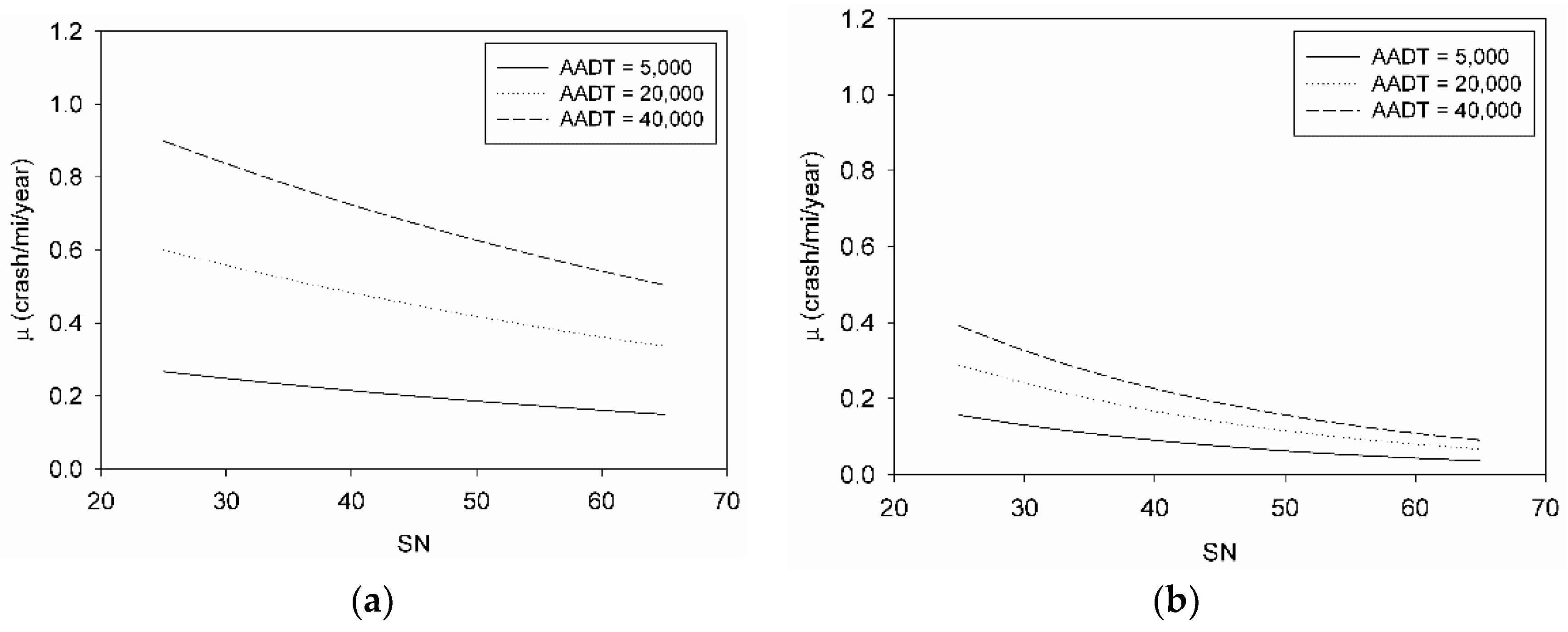
To contrast the impact of pavement surface condition on the traffic safety under various environmental surface conditions, NB regression models were derived for crashes occurring in dry and wet conditions. Figure 7 shows that these models included the SN as an explanatory variable, where the crash rate decreases as the SN increases. The higher dispersion coefficient for the wet model compared to the dry one indicates that the variability in the wet crash records increases on sections with higher crash rates. Furthermore, the wet model had a higher decay rate for increasing SN; however, the overall crash rates for the wet model are lower than those for dry conditions. This reduction of crash rates under wet conditions cannot be explained using the explanatory variables in the study. The sparseness in wet crash records reflects the complexity of wet crash events and the need for extensive investigations to understand the effects and contrast between varying environmental conditions.
4.3. Risk Analysis Results
To describe the risk level of roadway departure crashes for the segments included in the study, elaborate probabilistic analysis was conducted based on the framework introduced in Section 3.2. The first part of the risk analysis focuses on evaluating the PMF of the number of crashes occurring on a segment with given conditions. Figure 8a,b present the PMFs (excluding the ) for various SN values and two AADT levels, with fixed IRI, and SL. The PMFs in Figure 8a,b were estimated using the fitted parameters for the general model provided in Table 1. The columns colors do not reflect the probability magnitude; rather, they are provided to enhance the contrast between the columns in the figure. From the figures, for lower SNs, the PMF has a heavier tail, meaning that higher crash numbers are more likely. Figure 8b shows that the probability of having one crash increases as the SN decreases, and peaks around SN = 35, before starting to decrease as the SN decreases. This does not indicate that sections with lower skid numbers had a lower probability of having a crash; it indicates that sections with lower SN had a higher probability of having more than one crash, which shifts the PMF mean. Figure 9 shows that the total probability of having at least one crash as a function of SN and AADT (and fixed IRI and SL values) increases as the SN decreases.
Figure 10a,b presents the complete PMF for dry and wet models. The models were shifted NB models, which start at 1 crash as the lowest possible number of crashes. From the figures, it can be seen that as the skid number decreases the probability of having one crash decreases; however, the probability of having more crashes increases. Figure 10a,b indicates that for dry crashes, there is a higher probability of observing more than one crash on the same segment as compared to wet crashes. This does not reflect the probability of observing crashes given the environmental surface conditions on a segment. To derive a PMF for observing crashes given the environmental surface conditions on a segment, full records throughout the year should be used to include all the days that had wet surface conditions and dry surface conditions, and then contrast the odds of having crashes in a wet day versus a dry day.
The risk space defined in Equation (5) defines all possible crash risks under the assumption that the fitted model is the true model. However, due to the higher dimensionality of the risk surfaces at higher crash numbers, the discussion will be limited to the first three risk surfaces in a risk space. Given the general model with the following fixed segment conditions: SN = 30, AADT = 20,000, IRI = 90 in/mi, and SL = 65, the probability projection of the risk surface at is a scaler (i.e., zero rank tensor) corresponding to . Moreover, the probability projection of the risk surface at is a vector (i.e., first rank tensor) of probabilities as shown in Figure 11a. Considering the scenario of two crashes happening on the same mentioned segment, the probability projection of the risk surface is a second rank tensor represented in Figure 11b. The sum of probabilities in Figure 11a is 0.27, which equals the probability of observing exactly one crash a year on the given segment, under the assumption that crash frequency is truly captured in the general model, regardless of the severity level (). Similarly, the sum of probabilities in Figure 11b is 0.12, which is equal to the probability of observing exactly two crashes a year on the same given segment (). The assumed distribution of severity levels in this study can be oversimplified; however, distributions that are more sophisticated require a different type of analysis, which is outside the scope of this study.
5. Conclusions
This study presented a thorough analysis of selected roadway departure crashes in Iowa between 2006 and 2016. All crash records were mapped onto one-mile segments with known AADT, SL, SN, IRI, and RD in a GIS database. The crash records were correlated to the pavement surface condition (i.e., SN, IRI, and RD) using NB regression models. Moreover, a novel risk analysis framework was introduced to perform crash risk assessment and evaluate the possible consequences for a given combination of events. The key conclusions from the study are:
- Crash records are sparse in nature and require carful modeling using discrete count models, such as the negative binomial repression model.
- For the general crash model, which included all crash events under various severities and environmental surface conditions, higher skid resistance reduced the roadway departure crash rates. This impact is amplified on segments with higher speed limits, which reflects the importance of adequate skid resistance on higher speed segments.
- For the general model, rougher road segments had slightly higher crash rates. This impact is amplified on segments with higher speed limits.
- Higher skid resistance reduced the crash rates for both wet and dry crashes.
- Exploring the distribution of the count number of crashes for a given section, provides extra information that cannot be captured by examining the average crash rates solely.
- The risk analysis of traffic crashes provides a helpful tool for estimating the expected consequences in terms of human injury, social impact, and monetary value.
- There is a need for further investigation to understand the impact of weather condition on traffic crashes, and the interaction between the pavement surface condition and weather conditions.
Author Contributions
A.A. conceived the study, developed the crash models, and devised the risk models and their mathematical construct. I.N. processed and organized the data records in the GIS database. O.S. provided guidance on the safety analysis and guided the team through the study and the manuscript development. C.A.M. reviewed the risk analysis section and the proposed concepts.
Funding
This research received no external funding.
Conflicts of Interest
The authors declare no conflict of interest.
References
- Blincoe, L.J.; Miller, T.R.; Zaloshnja, E.; Lawrence, B.A. The Economic and Societal Impact of Motor Vehicle Crashes, 2010; Report No. DOT HS 812 013; National Highway Traffic Safety Administration: Washington, DC, USA, 2015.
- Tighe, S.; Li, N.; Falls, L.; Haas, R. Incorporating Road Safety into Pavement Management. Transp. Res. Rec. J. Transp. Res. Board 2000, 1699, 1–10. [Google Scholar] [CrossRef]
- Jung, S.; Jang, K.; Yoon, Y.; Kang, S. Contributing factors to vehicle to vehicle crash frequency and severity under rainfall. J. Saf. Res. 2014, 50, 1–10. [Google Scholar] [CrossRef] [PubMed]
- Hussein, N.A.; Hassan, R.A.; Evans, R. Assessing the Impacts of Pavement Surface Condition on the Performance of Signalized Intersections. In Proceedings of the 9th International Conference on Managing Pavement Assets, Washington, DC, USA, 18–21 May 2015. [Google Scholar]
- Vinayakamurthy, M. Effect of Pavement Condition on Accident Rate. Masters’ Thesis, Arizona State University, Tempe, AZ, USA, 2017. [Google Scholar]
- Cowe Falls, L.; Ibrahim, A. Development of a Safety Management System (SMS) for the Nova Scotia Department of Transportation and Public Works. In Proceedings of the 2000 Annual Conference and Exhibition of the Transportation Association of Canada, St. John, NB, Canada, 1–4 October 2000. [Google Scholar]
- Henry, J.J. Evaluation of Pavement Friction Characteristics; Transportation Research Board: Washington, DC, USA, 2000; Volume 291, ISBN 0309068746. [Google Scholar]
- Noyce, D.A.; Bahia, H.U.; Yambo, J.M.; Kim, G. Incorporating Road Safety into Pavement Management: Maximizing Asphalt Pavement Surface Friction for Road Safety Improvements; Midwest Regional University Transportation Center: Madison, WI, USA, 2005. [Google Scholar]
- Hall, J.W.; Smith, K.L.; Titus-Glover, L.; Wambold, J.C.; Yager, T.J.; Rado, Z. NCHRP Web-Only Document 108: Guide for Pavement Friction. National Cooperative Highway Research Program; Transportation Research Board National Academy: Washington, DC, USA, 2009. [Google Scholar]
- Persson, B.N.J. Theory of rubber friction and contact mechanics. J. Chem. Phys. 2001, 115, 3840–3861. [Google Scholar] [CrossRef] [Green Version]
- Persson, B.N.J. Contact mechanics for randomly rough surfaces. Surf. Sci. Rep. 2006, 61, 201–227. [Google Scholar] [CrossRef] [Green Version]
- Pardillo Mayora, J.M.; Jurado Piña, R. An assessment of the skid resistance effect on traffic safety under wet-pavement conditions. Accid. Anal. Prev. 2009, 41, 881–886. [Google Scholar] [CrossRef] [PubMed]
- Buddhavarapu, P.; Banerjee, A.; Prozzi, J.A. Influence of pavement condition on horizontal curve safety. Accid. Anal. Prev. 2013, 52, 9–18. [Google Scholar] [CrossRef] [PubMed]
- Musey, K.; Park, S. Pavement Skid Number and Horizontal Curve Safety. Procedia Eng. 2016, 145, 828–835. [Google Scholar] [CrossRef]
- Neuman, T.R.; Pfefer, R.; Slack, K.L.; Hardy, K.K.; Council, F.; McGee, H.; Prothe, L.; Eccles, K. A Guide for Addressing Run-Off-Road Collisions. In NCHRP Report 500: Guidance for Implementation of the AASHTO Strategic Highway Safety Plan; Transportation Research Board National Academy: Washington, DC, USA, 2003; Volume 6. [Google Scholar]
- Torbic, D.J.; Harwood, D.W.; Gilmore, D.K.; Pfefer, R.; Neuman, T.R.; Slack, K.L.; Hardy, K.K. A Guide for Reducing Collisions on Horizontal Curves. In NCHRP Report 500: Guidance for Implementation of the AASHTO Strategic Highway Safety Plan; Transportation Research Board National Academy: Washington, DC, USA, 2004; Volume 7. [Google Scholar]
- Merritt, D.K.; Lyon, C.A.; Persaud, B.N. Evaluation of Pavement Safety Performance; The National Academies of Sciences, Engineering, and Medicine: Washington, DC, USA, 2015. [Google Scholar]
- McGee, H.W.; Hanscom, F.R. Low-cost treatments for horizontal curve safety. In Proceedings of the ITE Annual Meeting and Exhibit Institute of Transportation Engineers, San Antonio, TX, USA, 9–12 August 2009. [Google Scholar]
- U.S. Department of Transportation Federal Highway Administration. Proven Safety Countermeasures, Enhanced Delineation and Friction for Horizontal Curves. Available online: https://safety.fhwa.dot.gov/provencountermeasures/enhanced_delineation/ (accessed on 4 April 2018).
- De Leon Izeppi, E.; Katicha, S.W.; Flintsch, G.W.; McCarthy, R.; McGhee, K.K. Continuous Friction Measurement Equipment as a Tool for Improving Crash Rate Prediction: A Pilot Study; Transportation Research Board: Washington, DC, USA, 2016. [Google Scholar]
- De León Izeppi, E.; Katicha, S.W.; Flintsch, G.W.; McGhee, K.K. Pioneering Use of Continuous Pavement Friction Measurements to Develop Safety Performance Functions, Improve Crash Count Prediction, and Evaluate Treatments for Virginia Roads. Transp. Res. Rec. J. Transp. Res. Board 2016, 2583, 81–90. [Google Scholar] [CrossRef]
- McCarthy, R.; Flintsch, G.W.; Katicha, S.W.; McGhee, K.K.; Medina-Flintsch, A. New approach for managing pavement friction and reducing road crashes. Transp. Res. Rec. J. Transp. Res. Board 2016, 23–32. [Google Scholar] [CrossRef]
- Najafi, S. Pavement Friction Management (PFM)—A Step toward Zero Fatalities. Ph.D. Thesis, Virginia Polytechnic Institute and State University, Blacksburg, VA, USA, 2016. [Google Scholar]
- Geedipally, S.R.; Pratt, M.P.; Lord, D. Effects of geometry and pavement friction on horizontal curve crash frequency. J. Transp. Saf. Secur. 2017, 1–22. [Google Scholar] [CrossRef]
- Start, M.; Kim, J.; Berg, W. Potential Safety Cost-Effectiveness of Treating Rutted Pavements. Transp. Res. Rec. J. Transp. Res. Board 1998, 1629, 208–213. [Google Scholar] [CrossRef]
- Ong, G.P.; Fwa, T.F. Wet-Pavement Hydroplaning Risk and Skid Resistance: Modeling. J. Transp. Eng. 2007, 133, 590–598. [Google Scholar] [CrossRef]
- Fwa, T.F.; Pasindu, H.R.; Ong, G.P. Critical Rut Depth for Pavement Maintenance Based on Vehicle Skidding and Hydroplaning Consideration. J. Transp. Eng. 2012, 138, 423–429. [Google Scholar] [CrossRef]
- Fwa, T.F.; Ong, G.P. Transverse Pavement Grooving against Hydroplaning. II: Design. J. Transp. Eng. 2006, 132, 449–457. [Google Scholar] [CrossRef]
- Ong, G.P.; Fwa, T.F. Transverse Pavement Grooving against Hydroplaning. I: Simulation Model. J. Transp. Eng. 2006, 132, 441–448. [Google Scholar] [CrossRef]
- Chan, C.Y.; Huang, B.; Yan, X.; Richards, S. Investigating effects of asphalt pavement conditions on traffic accidents in Tennessee based on the pavement management system (PMS). J. Adv. Transp. 2010, 44, 150–161. [Google Scholar] [CrossRef]
- Žuraulis, V.; Levulytė, L.; Sokolovskij, E. The impact of road roughness on the duration of contact between a vehicle wheel and road surface. Transport 2014, 29, 431–439. [Google Scholar] [CrossRef]
- Road Safety. Road Safety Annual Report, 1972; Catalogue Number T45-1/1972; Transport Canada: Ottawa, ON, Canada, 1973.
- ASTM International. ASTM E274/E274M-15 Standard Test Method for Skid Resistance of Paved Surfaces Using a Full-Scale Tire; ASTM International: West Conshohocken, PA, USA, 2015. [Google Scholar] [CrossRef]
- Salem, O.; AbouRizk, S.; Ariaratnam, S. Risk-based life-cycle costing of infrastructure rehabilitation and construction alternatives. J. Infrastruct. Syst. 2003, 9, 6–15. [Google Scholar] [CrossRef]
- American Association of State Highway and Transportation Officials (AASHTO). Highway Safety Manual; American Association of State Highway and Transportation Officials: Washington, DC, USA, 2010; ISBN 9781560514770 1560514779. [Google Scholar]
- Bradlow, E.T.; Hardie, B.G.S.; Fader, P.S. Bayesian inference for the negative binomial distribution via polynomial expansions. J. Comput. Graph. Stat. 2002, 11, 189–201. [Google Scholar] [CrossRef]
- JMP®, Version 12; SAS Institute Inc.: Cary, NC, USA, 1989–2007.
Figure 1.
A screenshot of the test output from a locked wheel trailer showing SN, rolling test tire speed, vehicle speed, and other test variables.
Figure 1.
A screenshot of the test output from a locked wheel trailer showing SN, rolling test tire speed, vehicle speed, and other test variables.

Figure 2.
The histogram for the pavement condition including (a) SN; (b) IRI; and (c) RD; for the segments included in the study.
Figure 2.
The histogram for the pavement condition including (a) SN; (b) IRI; and (c) RD; for the segments included in the study.

Figure 3.
The histogram of (a) the severity levels for the roadway departure crashes and (b) the weather-related surface condition during the crash events.
Figure 3.
The histogram of (a) the severity levels for the roadway departure crashes and (b) the weather-related surface condition during the crash events.
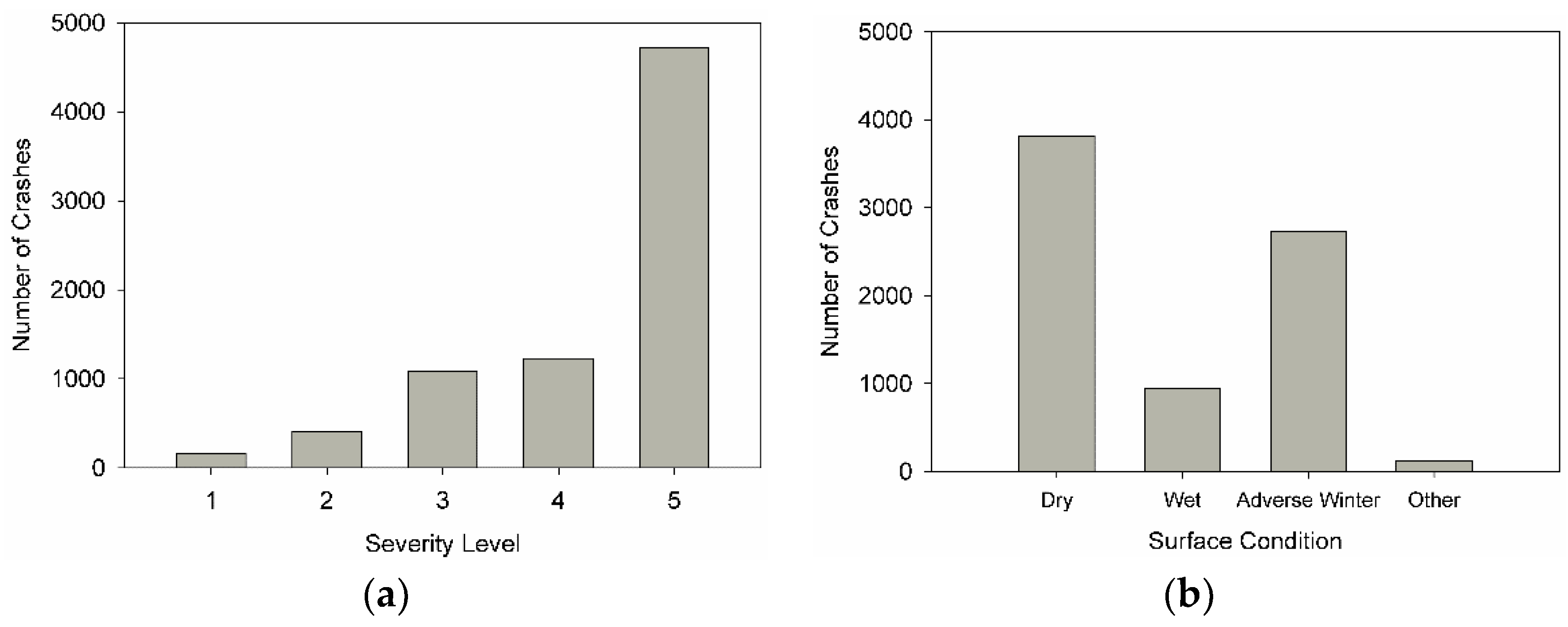
Figure 4.
The empirical trends between the average number of crashes and (a) The traffic volume expressed in AADT; and (b) the speed limit for all segments in the study.
Figure 4.
The empirical trends between the average number of crashes and (a) The traffic volume expressed in AADT; and (b) the speed limit for all segments in the study.

Figure 5.
The empirical trends between the average number of crashes and (a) SN; (b) IRI; and (c) RD.
Figure 5.
The empirical trends between the average number of crashes and (a) SN; (b) IRI; and (c) RD.


Figure 6.
Expected crash rates as a function of SN, AADT, and SL; as explained by the NB regression models.
Figure 6.
Expected crash rates as a function of SN, AADT, and SL; as explained by the NB regression models.
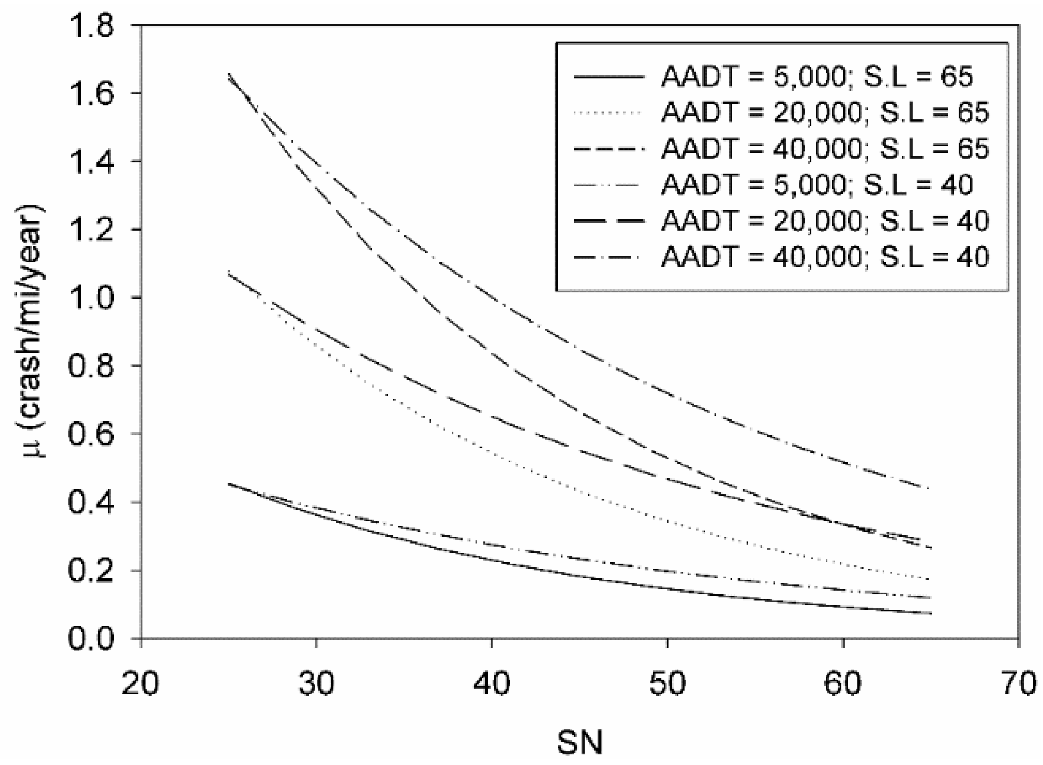
Figure 7.
Expected crash rates as a function of SN, AADT, and SL; as explained by the NB regression models for (a) dry and (b) wet environmental surface conditions.
Figure 7.
Expected crash rates as a function of SN, AADT, and SL; as explained by the NB regression models for (a) dry and (b) wet environmental surface conditions.

Figure 8.
Probability mass function using fitted general model parameters for varying SN; (a) 20,000 AADT and (b) 40,000 AADT; and fixed IRI and SL.
Figure 8.
Probability mass function using fitted general model parameters for varying SN; (a) 20,000 AADT and (b) 40,000 AADT; and fixed IRI and SL.
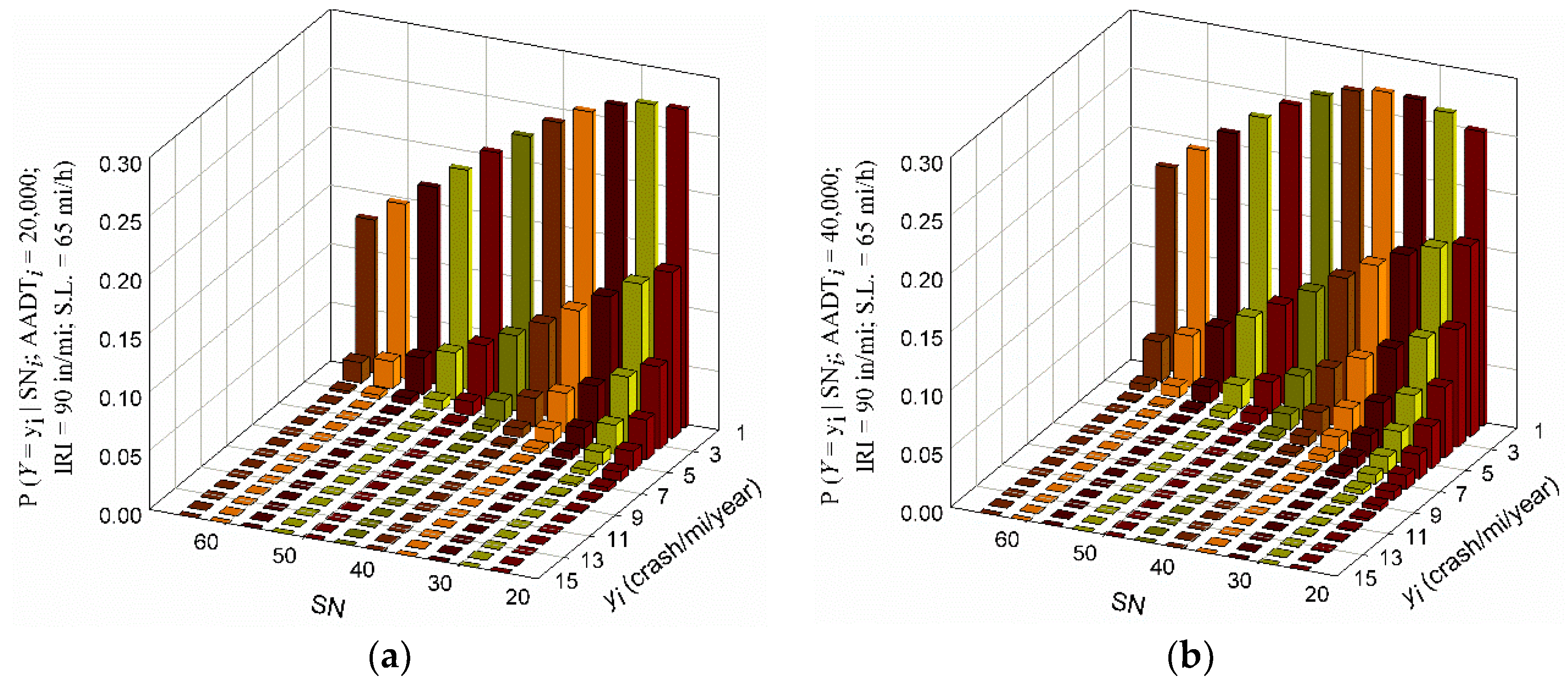
Figure 9.
Probability of having at least one crash as a function of SN and varying AADT for the fitted general model.
Figure 9.
Probability of having at least one crash as a function of SN and varying AADT for the fitted general model.
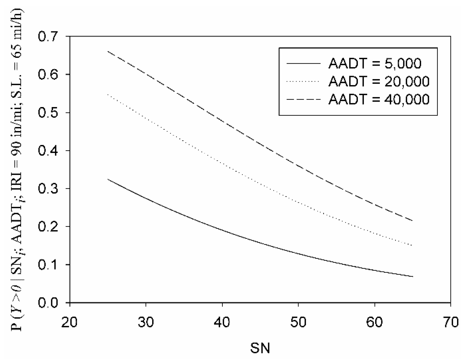
Figure 10.
Probability mass function under varying SN and fixed AADT for (a) dry and (b) wet fitted models.
Figure 10.
Probability mass function under varying SN and fixed AADT for (a) dry and (b) wet fitted models.
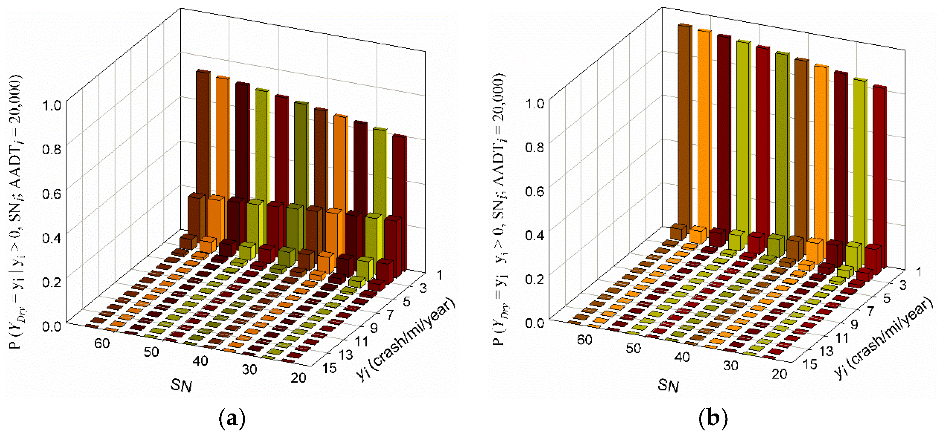
Figure 11.
Probability of having (a) one crash a year with various severity levels and (b) two crashes a year with various severity combinations.
Figure 11.
Probability of having (a) one crash a year with various severity levels and (b) two crashes a year with various severity combinations.


Table 1.
Statistical summary of all fitted NB regression models.
| Model Name | NB Regression Form | Explanatory Variables Statistical Summary | ||||
|---|---|---|---|---|---|---|
| Term | Estimate 2 | Std. Error | Wald Chi-Square | p-Value | ||
| General Model | 2.67 × 10⁻³ | 0.225 | 696.93 | <0.01 | ||
| 6.22 × 10⁻¹ | 0.019 | 1103.51 | <0.01 | |||
| −1.29 × 10⁻² | 0.002 | 43.62 | <0.01 | |||
| 1.57 × 10⁻³ | <0.001 | 19.34 | <0.01 | |||
| −5.06 × 10⁻⁴ | <0.001 | 5.32 | 0.02 | |||
| 1.44 × 10⁻⁴ | <0.001 | 14.64 | <0.01 | |||
| Dry Condition 1 | 2.67 × 10⁻³ | 0.593 | 99.87 | <0.01 | ||
| 5.83 × 10⁻¹ | 0.047 | 153.45 | <0.01 | |||
| −1.45 × 10⁻² | 0.005 | 8.40 | <0.01 | |||
| Wet Condition 1 | 9.18 × 10⁻³ | 1.497 | 9.82 | <0.01 | ||
| 4.41 × 10⁻¹ | 0.122 | 12.99 | <0.01 | |||
| −3.66 × 10⁻² | 0.013 | 7.56 | <0.01 | |||
1 The model was derived using the shifted NB distribution; 2 Std. Error: the standard error value of the fitted parameter βj.
© 2018 by the authors. Licensee MDPI, Basel, Switzerland. This article is an open access article distributed under the terms and conditions of the Creative Commons Attribution (CC BY) license (http://creativecommons.org/licenses/by/4.0/).
Share and Cite
MDPI and ACS Style
Alhasan, A.; Nlenanya, I.; Smadi, O.; MacKenzie, C.A. Impact of Pavement Surface Condition on Roadway Departure Crash Risk in Iowa. Infrastructures 2018, 3, 14. https://0-doi-org.brum.beds.ac.uk/10.3390/infrastructures3020014
AMA Style
Alhasan A, Nlenanya I, Smadi O, MacKenzie CA. Impact of Pavement Surface Condition on Roadway Departure Crash Risk in Iowa. Infrastructures. 2018; 3(2):14. https://0-doi-org.brum.beds.ac.uk/10.3390/infrastructures3020014
Chicago/Turabian StyleAlhasan, Ahmad, Inya Nlenanya, Omar Smadi, and Cameron A. MacKenzie. 2018. "Impact of Pavement Surface Condition on Roadway Departure Crash Risk in Iowa" Infrastructures 3, no. 2: 14. https://0-doi-org.brum.beds.ac.uk/10.3390/infrastructures3020014