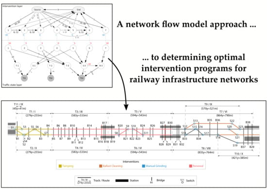
A Network Flow Model Approach to Determining Optimal Intervention Programs for Railway Infrastructure Networks

Abstract

The determination of the optimal interventions to execute on rail infrastructure networks is a challenging task, due to the many types of objects (e.g., bridges, tracks, and switches), how the objects work together to provide service, and the possible reductions in costs and service disruptions as obtained by grouping interventions. Although railway infrastructure managers are using computer systems to help them determine intervention programs, there are none that result in the highest net benefits while taking into consideration all of these aspects. This paper presents a network flow model approach that allows for determining the optimal intervention programs for railway infrastructure networks while taking into considerations different types of objects, how the objects work together to provide service, and object and object-traffic dependencies. The network flow models are formulated as mixed integer linear programs, where the optimal intervention program is found by using the simplex and branch and bound algorithms. The modelling approach is illustrated by using it to determine the optimal intervention program for a 2200 m multi-track railway line consisting of 11 track sections, 23 switches, and 39 bridges. It is shown that the proposed constrained network flow model can be used to determine the optimal intervention program within a reasonable amount of time, when compared to more traditional models and search algorithms.

1. Introduction

Railways are used to transport large numbers of passengers and large amounts of goods at specified speeds. As railway infrastructure networks deteriorate over time, interventions have to be executed in order to be able to provide an adequate level of service over time. When executed, these interventions cost owners a considerable amount of money and they normally result in disruptions to service. If they are not executed, failures will eventually occur, which will also result in intervention costs and disruptions to service. The determination of the optimal combination of interventions to execute in an upcoming planning period is challenging due to the need of considering all objects,

• the costs of the interventions for both the owner and the users of the network, which vary depending on the time of execution (e.g., night, day) and the possibility to group interventions together, and
• the benefits of the interventions in terms of risk reduction for both the owner and the user, i.e., the probability and consequence of failures.

Although railway infrastructure managers are using computer systems to help them determine intervention programs, there are none that result in the highest net benefits take into consideration all of these aspects. Most of these systems, and research done to support the development of these systems, have predominantly either, (1) considered only the costs and benefits of executing interventions on objects of one type, e.g., tracks; (2) neglected the variations in the costs and disruptions to the service of grouping interventions of different types; or (3) both. Without an appropriate model, railway managers are unable to determine the optimal intervention programs.

This paper proposes a network flow model approach that overcomes this problem as it allows determining optimal intervention programs for railway infrastructure networks while taking into consideration;

• different types of objects,
• how the objects work together to provide service,
• dependencies between objects, and
• object-traffic dependencies.

Using constrained network flow models as proposed in this paper overcomes this problem. They allow for the determination of the optimal intervention programs for railway infrastructure networks while taking into considerations different types of objects, how the objects work together to provide service, and object and object-traffic dependencies. The optimal intervention program is the one that has the maximum net benefit, i.e., the difference between the reductions in risks due to the execution of interventions minus the costs. The models consist of an intervention layer, which enables the selection of the interventions and consideration of the object dependencies, and a traffic state layer, which enables the modelling of how the network provides service and the object-traffic dependencies. To ensure the models work constraints are required. They include flow conservation constraints to ensure consistency in the model and side constraints, which ensure that the real world is realistically modelled. The side constraints include (1) source flow constraints to enable modelling the durations of interventions; (2) topological constraints to enable the introduction of topological dependencies; (3) exclusivity constraints to ensure that multiple interventions are not executed on the same object in the same time period; (4) organisational constraints to ensure that external limitations, e.g., budget are not exceeded; and (5) structural constraints to ensure that mandatory interventions are executed if required. The network flow models are formulated as mixed integer linear problems. They are solved while using the simplex method and the branch and bound algorithm.

The modelling approach is illustrated by using it to determine the optimal intervention program for a 2200 m multi-track railway line, which consists in addition to the 11 track sections of 23 switches and 39 bridges. The efficiency and effectiveness of the model are demonstrated by comparing the determination of this intervention program with the ones determined while using a reduced exhaustive search algorithm and an algorithm based on simplified decision rules. It is shown that the proposed constrained network flow model and search algorithm can be used to determine the optimal intervention program within a reasonable amount of time.

The remainder of this paper is structured as follows: Section 2 includes a literature review. Section 3 includes a description of the problem and its components. Section 4 includes a description of the constrained network flow models in both general terms and mathematically. Section 5 includes the example. Section 6 includes the comparisons of the optimal intervention programs determined while using the three different approaches. Section 7 includes a discussion and the conclusions of the work.

2. Literature Review

Research focused on the best ways to plan interventions has increased in recent years. The research can be grouped into three general categories. In category 1, researchers have focused on determining optimal intervention strategies, i.e., the determination of the optimal interventions to be executed on specific objects over their life cycles if there are no external constraints [1,2,3,4]. In category 2, researchers have focused on determining optimal intervention programs, i.e., the determination of the optimal interventions to execute on many objects taking into consideration the current state of the objects, the optimal intervention strategies of all objects, and external constraints, e.g., [5,6,7,8,9,10,11,12,13]. In category 3, researchers have focused on how to group interventions on objects once it is known the work that needs to be executed, e.g., [14,15,16]. Although categories 1 and 3 are interesting, they are not directly related to the work that is presented in this article, and are, therefore, not followed further.

The research conducted in category 2 can be further divided into research using a bottom-up approach, a top-down approach and using an integrated approach. Using the bottom-up approach, researchers determine the interventions to be executed for each object individually, i.e., without consideration of other objects or constraints on the development of intervention programs, and then modify these interventions to take into consideration reductions in cost and service disruptions of executing interventions on multiple objects of the same type simultaneously. Using the top-down approach, researchers determine where track occupancy schedules are required without detailed consideration of individual objects and then determine the interventions that should be executed on the objects within the affected area. Using an integrated approach, researchers directly determine the interventions to be executed on objects of different types while taking into consideration the possible reductions in costs and disruptions to service of executing multiple interventions simultaneously.

Of the researchers that have used a bottom-up approach, which is more common, most have focused on the determination of the optimal intervention programs for tracks, e.g., [5,6,7,8,9]. Caetano & Teixeira [6] determined optimal and near-optimal interventions to be executed for each object individually, before developing the intervention program for multiple adjoined railway segments while using penalty costs for moving away from the optimal point in time for the execution of interventions. The interventions to be executed were determined using a mixed integer linear program. Furuya & Madanat [8] incorporated economies of scale and capacity constraints in order to consider economical, functional, and stochastic dependencies between different objects in the network in order to determine the interventions to be executed with a two-stage approach. Zhao et al. [5] developed a genetic algorithm-based approach for synchronising the interventions of different components within a track section. They simplified the combinatorial complexity by using three standard combinations. Fecarotti & Andrews [7] developed intervention programs for an entire network by selecting the intervention strategy to follow for each object out of different strategies evaluated using Petri-Net simulations. Pargar [9] used a linear integer program to determine the optimal time point for executing interventions on different track components considering dependencies between different components through component and location specific setup costs, and between different track sections through a system dependent setup cost. An area of improvement on this research, however, is the consideration of the reduction in costs and service disruptions of executing interventions on multiple objects of different types (e.g., track, switches, level crossing, and bridges).

The researchers that have used a top-down approach have all focused on the grouping of interventions on different types of objects within time-free periods, which are determined by the models [10,11,12,13]. Den Hertog et al. [10], extended by Van Zante-De Fokkert et al. [13], used a maximum work zone length and a time of the day constraint to develop optimal intervention work zones for railway infrastructure networks in order to minimise the service disturbance and costs. In the second step, the work zones were assigned to particular nights when considering the possible combinations of work zones over the network. Jenema [11] developed a train-free period planning approach that is based on a linear integer program for minimising the required track capacity for executing interventions. They considered the trade-off between higher intervention costs and lower possession costs for a night execution compared with a day execution. Lethanh & Adey [12] assumed that managers of a railway line passing through different countries would need to agree on fixed windows of intervention time in the future without knowing which intervention that they would need to execute exactly, and used a real options approach to determine the optimal window for each rail manager.

The researchers that have used an integrated approach have all focused on directly estimating the owner costs of interventions and the user costs of service disruption while taking into consideration the reductions in costs and service disruptions by executing interventions simultaneously. For example, Burkhalter et al. [17] estimated the object level owner costs together with the network level user costs without the requirement of an iterative process or a multi-step model, by using faults to connect the owner costs of interventions with the user costs that are related to states of the network. An integer non-linear program was used to determine the optimal intervention program. Hajdin & Adey [18], extended by Eicher et al. [19] and Lethanh et al. [20], developed a network model for developing optimal intervention programs for road networks while taking into account cost variations by executing intervention on neighbouring objects, spatial constraints, and a budget limitation. Their network model searched for the path with the lowest cost along a network, and was formulated as an integer linear program. The approach that is presented in this paper, is based on this work. The approach to modelling enables the development of similar models that are capable of determining optimal intervention programs for railway infrastructure networks. The adaptations have also enabled the mathematical models to be linear, instead of non-linear, as the one presented in [17].

3. Problem Set-Up

3.1. Optimal Intervention Program

The optimal intervention program is the one that yields the maximum net benefit measured as the difference between the reduction in the risks and the intervention costs for both the owner and the users of the network (Equation (1)), and fulfils all constraints, e.g., budget and externally mandated interventions.

$$MaxZ=Benefit-Costs=\left(R_0-R_{IP}\right)-\left(C_{O,IP}+C_{U,IP}\right)$$

(1)

where

• R₀ represents the risks, i.e., the probability of failure multiplied by the consequences of failure, when no interventions are executed,
• R_IP represents the risks when all interventions in intervention program IP are executed,
• C_O,IP represents the owner costs of interventions in intervention program IP, and
• C_U,IP represents the user costs that are related to service disruptions due to interventions in intervention program IP.

Owner costs are estimated as the sum of fixed and variable costs (Equation (2)), where it is assumed that the magnitude of the fixed costs per intervention are dependent on the number, and type, of interventions executed together, i.e., in groups.

$$C_{O,IP}={\displaystyle \sum }_{g=1}^G{c}_{fix,g}+{\displaystyle \sum }_{i=1}^I{c}_{variable,i}$$

(2)

where

• c_fix,g represents the fixed owner costs summed over all intervention groups g, and
• c_variable,i represents the variable owner costs summed over all interventions i.

The user costs are estimated as the sum of service disruption costs that are associated with the traffic states, i.e., combination of open and closed routes during a specific time of the week, required during the execution of the interventions in intervention program IP (Equation (3)).

$$C_{U,IP}={\displaystyle \sum }_{ts=1}^{TS}\left(LLO{S}_{ts}\ast Duratio{n}_{ts}\ast VOT\right)$$

(3)

where

• LLOS_ts represents the total increased travel time per unit time due to traffic state ts,
• Duration_ts represents the length of time the traffic state ts is required, and
• VOT represents the value of travel time.

3.2. Topological Structure

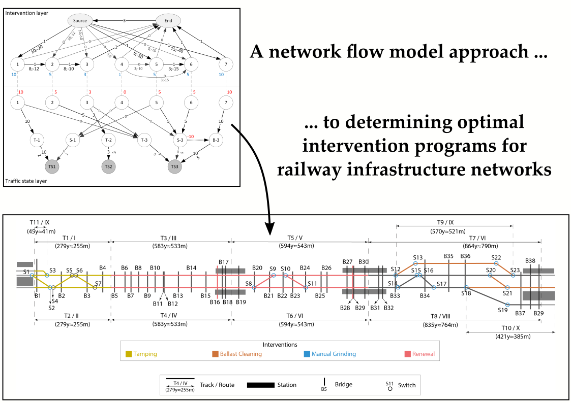
In the proposed model the network is composed of lines, which consist of all infrastructure objects between two stations (Figure 1). Each line is divided into routes, which are further divided into sections by the location of switches. Trains are able to change routes at switch location. Infrastructure objects are assigned to the route(s) where they enable the flow of traffic.

3.3. Intervention Types

Interventions are classified as shown in

Table 1. Intervention types.

Intervention Type	Intervention Is … Track Clearance Area	During the Intervention, … Track Occupancy Is Required	During the Intervention, Service Is …	Example Reasons
A	inside	extensive	affected	use of intervention trains for continuous track replacement
B	inside	local	affected	location of work, position of machines for switch replacements, bridge renewals, level crossing renewals
C	outside	none	affected	closing track for the replacement of power supply cables
D	inside	local	not affected	local track interventions that can be executed be executed between the passing of trains in the normal train schedule
E	outside	no	not affected	replacing the lighting in train stations

while using, (1) the extent of the required track occupancy, i.e., is it necessary to close the entire route, just the track section, or is no closure required, and (2) operational impact, i.e., is it necessary to close the track to service during the execution of an intervention.

3.4. Dependencies

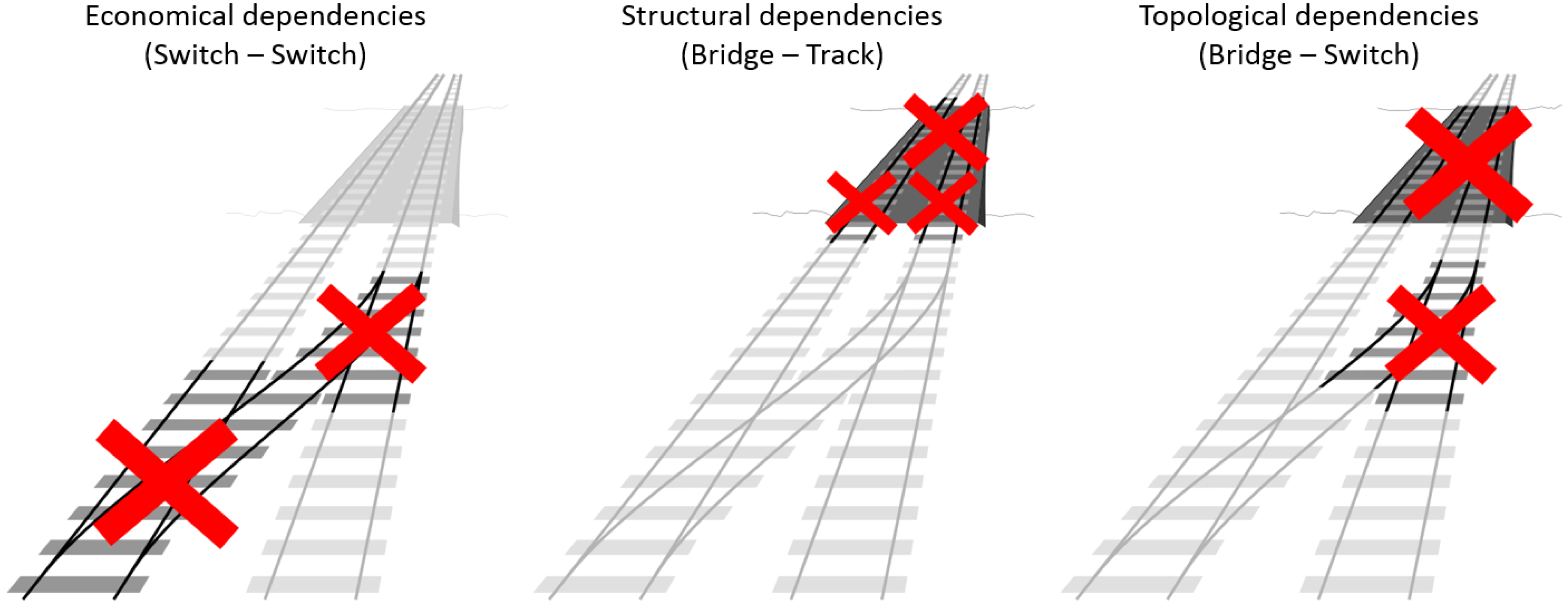
Four of the five types of dependencies, as identified in literature [8,21], are considered in the model (

Table 2. Dependencies.

Dependency	Refers to…	Example
Economical	the costs of executing an intervention being affected by the execution of other interventions	The costs for interventions on two different switches that lie close to each other are less if they are executed within the same shift than if they are executed at two different moments in time.
Structural	the ability of one object to function being physically affected by interventions on another object (also known as technical dependencies)	A rebuild of a bridge entails the rebuild of the carrying track infrastructure.
Topological	the ability of an object to provide service being dependent on other objects providing service (also known as performance oriented dependencies)	A switch cannot provide adequate service during a bridge intervention that requires a closure of the line. The overall duration of service disturbance can be reduced by a simultaneously execution of interventions on both objects.
Resource	the limits on used resources on multiple objects	The total intervention costs cannot surpass the available budget.

). Stochastic dependencies that exist when probabilities of object failures are correlated, e.g., due to common cause failures, are not considered. This paper considers risk on the object level. Stochastic dependencies, however, would require the risk estimation on the network level, which increases the combinatorial complexity significantly [22]. The economical, technical and topological dependencies are depicted in Figure 2.

4. Constrained Network Flow Models

4.1. Description

A constrained network flow model approach is proposed to determine the optimal intervention programs for railway infrastructure networks. Network models are often used to solve combinatorial optimisation problems [23,24]. In general, a network flow model is a representation of a real world situation that is depicted as a set of nodes that are connected by edges, where something flows from a source node, or source nodes, to a sink node, or sink nodes. The objective is often either, (1) to maximise the flow in the network or in parts of the network or, (2) to minimise the costs or distances of travel between multiple nodes in the network. In its simplest form, the flows in a network flow model are only constrained by the capacity constraints on each edge and by the flow conservation constraints on each node [23,25]. Some examples of well-known network flow problems are the assignment problem [26], shortest path [27], maximum flow problem [28], or minimum cost flow problem [25].

More complex network flow models are required to solve more complex problems. The job to machine problem, which transform the binary assignment of a job to a machine into the duration of the machine occupancy [25], or the maximum flow problem with gains along the network [29], require the relaxation of the flow conservation constraints in order to allow for gains and losses along the edges. Multi-commodity flow problems require independent flow conservation constraints for each commodity, while overall coupled constraints and the objective function couple the different commodities. In the traffic assignment problem, for example, the flow on each original-destination pair is represented by a separate commodity, which together share the capacity constraints of the edges [30]. A constrained shortest path problem introduces additional side constraints to the original shortest path problem, i.e., the shortest path with costs below a maximal budget [31].

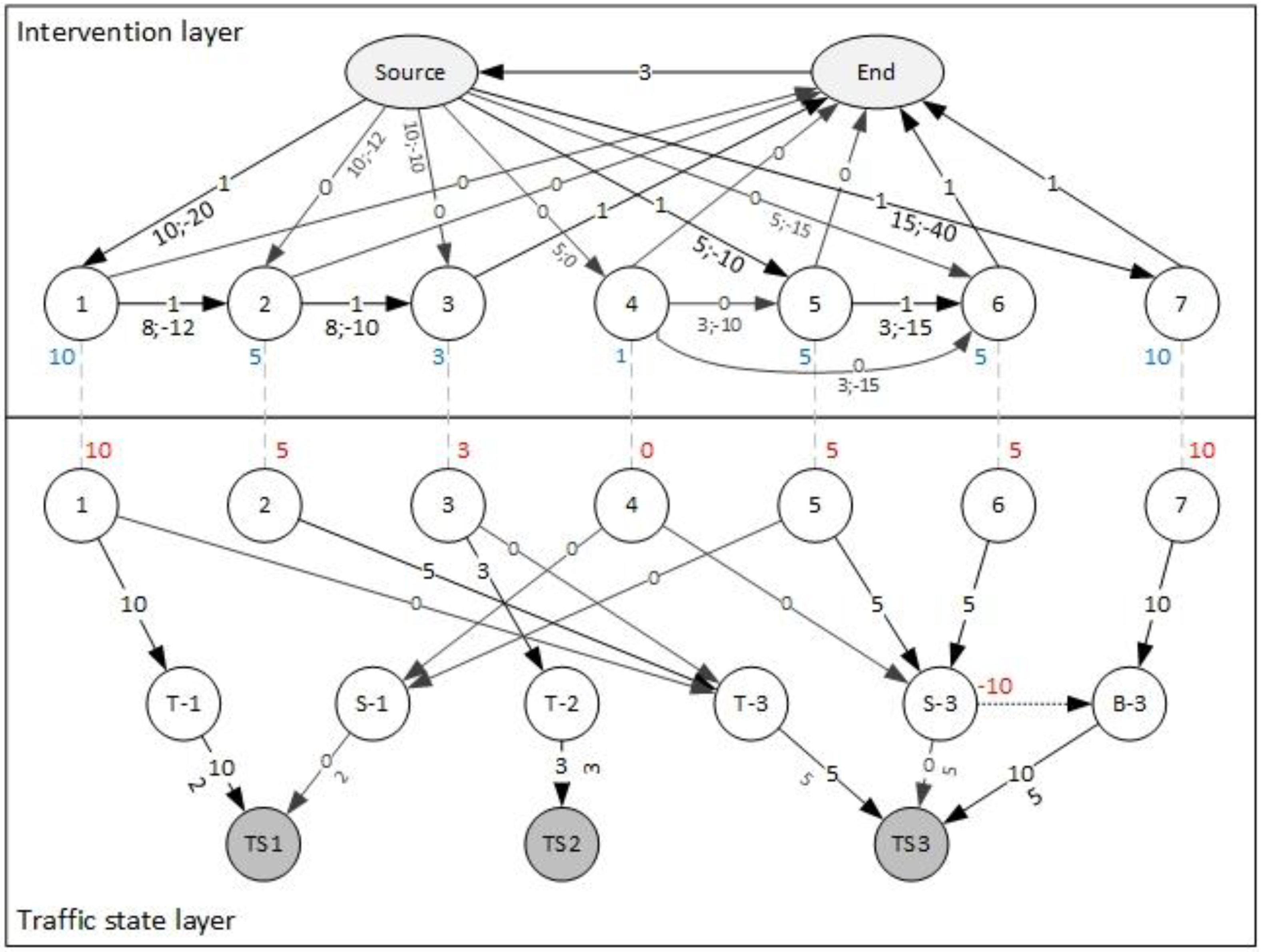
The constrained network flow approach that is proposed in this paper uses side constraints to take into consideration the structural, topological, and resource dependencies. The models consist of an intervention layer and a traffic state layer. The part of the network flow model within the intervention layer, is used to select the interventions to be executed and model the economical dependencies. It contains information on (1) the possible interventions; (2) the selected interventions; (3) the costs and benefits directly related to the interventions; and (4) the economical dependencies of the interventions.

The part of the network flow model within the traffic state layer is used to estimate the required duration of each traffic state and the service disruption to networks users when the selected interventions are executed, taking into consideration the topological dependencies. It contains information on (1) the possible traffic states; (2) the duration each traffic state is in place in order to execute the interventions; (3) the costs that are related to the traffic states; and (4) the topological dependencies of the interventions.

The model is illustrated in Figure 3 while using a small example consisting of seven possible interventions on objects that can be executed in one of three possible traffic states. Each numbered node in the intervention layer represents one particular intervention on one particular object. The numbers on the edges in the intervention layer represent the interventions that are included in the intervention program (for example, the 1 on the edge between the source node and node 1 means that there will be an intervention on object 1). The black numbers adjacent to the edges are the costs and benefits obtained by execution of the interventions. Costs are positive. Benefits are negative. (For example, the 10 on the edge between the source node and node 1 means that the intervention on object 1 will cost 10 monetary units (mu), and the −20 means that there will be 20 mu in benefits). The blue numbers below the nodes in the intervention layer indicate the duration of the interventions if they were selected (for example, the 10 below node 1, indicates that the intervention will take 10 time units (tus)).

The numbers on the edges in the traffic state layer indicate the amount of time a specific traffic configuration is to be in place (for example, the 10 on the edge between node 1 and node T − 1 in the traffic state layer means that intervention 1 when included in intervention group 1 will take 10 time units, and the 10 on the edge between node T − 1 and the node TS1 means that the execution of interventions in intervention group T − 1 will together require 10 tus). The red numbers above the nodes in the traffic state layer indicate the intervention duration required while taking into consideration whether they are selected and are shown as source flows in the traffic state layer. (For example, the blue number 1 under node 4 in the intervention layer indicates that this intervention would take 1 tu if selected, but since it is not selected, which can be seen by the 0 on the edge between the source node and node 4 in the intervention layer, this intervention requires 0 tus, which is indicated by the red 0). Each component of the model is explained in more detail in

Table 3. Meaning of components of the model in the intervention layer.

Node/Edge	Symbol	Represents	Example
An intervention node	$v^I$	a possible intervention on a specific object.
An edge from the source node to an intervention node	$e_{S,v}$	the inclusion of the intervention in the intervention program independent of other interventions, with full costs, i.e., both the fixed and variable parts, and full benefits.	$e_{S,3}$ represents the inclusion of intervention 3 independent of other interventions, with costs of 10 mus and benefits of −10 mus.
An edge from one intervention node to another	$e_{u,v}$	the inclusion of the intervention in the intervention program once another intervention has already been included, with only the variable part of the costs, and full benefits, i.e., it has been included only due to its “economical dependency”.	$e_{2,3}$ represents the inclusion of intervention 3 when intervention 2 has already been included, with costs of 8 mus (i.e., the variable part) and benefits of −10 mus.
An edge between an intervention node and an end node	$e_{v,E}$	nothing physical, but are used to enable the network flow model to function. As these edges do not contribute to the cost function, their cost values are 0.	An $e_{6,E}$ of 1 indicates that intervention 6 is included without the consideration of further economical dependant interventions.
The edge between the end and the source node	$e_{E,S}$	nothing physical, but is used to enable the network flow model to function. As this edge does not contribute to the cost function, its cost value is 0.	An $e_{E,S}$ of 3 indicates the inclusion of three economically independent groups.

and

Table 4. Meaning of components of the model in the traffic state layer.

Node/Edge	Symbol	Represents	Example
An intervention node	$v^{TS-i}$	a possible intervention on an object. Each intervention node in the traffic layer corresponds to one in the intervention layer.
A group node	$v^{TS-g}$	all interventions that are grouped together, i.e., can be executed by the same work team with the same traffic state.	Node S − 1 refers to the group of switch interventions executed in traffic state 1.
A traffic state node	$v^{TS-ts}$	a traffic state and acts as an end node within this layer.	Node TS1 refers to the end node of traffic state 1.
An edge between an intervention node and a group node	$e_{i,g}$	the amount of time required to execute an intervention which is included in an intervention group. As these durations do not contribute to the cost function, the cost values of these edges are 0.	An $e_{1,T-1}$ of 10 indicates that group T − 1, which refers to the track group in traffic state 1, is required for 10 time units to execute intervention 1.
An edge between a group node and a traffic state node	$e_{g,ts}$	the amount of time that a traffic state needs to be in place when executing the interventions belonging to the intervention group.	An $e_{T-1, TS1}$ of 10 indicates that group T − 1 requires traffic state 1 for 10 tus, with costs of 2 mus per tus.
An edge between two group nodes (dotted edge)	$e_{g1,g2}$	the number of time units that interventions in one intervention group can be executed simultaneously with interventions in another group.	An $e_{S-3,B-3}$ of 10 indicates that the total sum of the intervention durations for all intervention in group S − 3 can be reduced by 10 because they can be executed simultaneously with interventions in group B − 3.

.

The flow through the model, i.e., the interventions in the intervention layer and the time required to execute intervention in the traffic state layer, is subject to

• flow conservation constraints, which are imposed on each node,
• binary constraints, which are imposed on each edge in the intervention layer, except the edge between the end and source node ($e_{E,S}$), which indicates the number of economical independent groups of interventions, and
• side constraints, which are imposed by the physical structure of the model, which are explained in

  Table 5. Model constraints.

  Type	Ensure that…	Example
  Constraints on intervention nodes in the traffic state layer	the correct amounts of time required for each intervention is used.	The 5 tus required for intervention 2 are equal to those required for intervention 2, if intervention 1 is selected (i.e., 0 for $e_{S,2}$ and 1 for $e_{1,2}$).
  Constraints on intervention group nodes in the traffic state layer	the time in which interventions in multiple groups can be executed simultaneously is correctly accounted for. (dotted edges).	The −10 on the intervention group node S − 3 ensures that the amount of time that interventions in S − 3 ($e_{S-3}$) can be executed at the same time as those in B − 3 ($e_{,B-3}$) are removed from the model.
  Topological constraint	the flows on all edges between different group nodes (dotted edges) reaching another intervention group node are at most as high as the outflow on the edge to a traffic state node.	The flow on the edge S − 3 to B − 3 (i.e., 10 tus) is at most as high as the flow on the edge B − 3 to TS3 (i.e., 10 tus).
  Budget constraint	Ensures that the intervention costs do not surpass the available budget.	The sum of all intervention costs cannot surpass the budget of 50 mus.
  Structural constraint	Ensures that all mandatory interventions of structural dependent objects are selected when an initial intervention is selected.	Intervention 1 has to be executed when intervention 7 is executed due to structural dependencies.
  Exclusivity constraint	Ensures that at most one intervention per object is selected.	The sum of $e_{S,3}$ and $e_{2,3}$ is smaller or equal to 1.

  .

4.2. Mathematical Formulation

This section contains the mathematical formulation of the constrained network flow model to determine the optimal intervention programs on railway infrastructure networks.

4.2.1. Objective Function

The objective function is the maximisation of the sum product of the flow on each edge and the net benefit on each edge if an intervention was executed (Equation (4)).

$$MaxZ={\displaystyle \sum }_{u\in V^I}{\displaystyle \sum }_{v\in V^I}{\delta }_{u,v}·N{B}_{u,v}+{\displaystyle \sum }_{u\in V^{TS}}{\displaystyle \sum }_{v\in V^{TS}}{\gamma }_{u,v}·N{B}_{u,v}$$

(4)

where

• ${\delta }_{u,v}$ are binary variables that are 1 if the edge between the nodes u and v in the intervention layer is part of the optimal path and 0 otherwise, except when for ${\delta }_{u,v}$ is ${\delta }_{E,S}$, the edge connecting the end and start nodes. ${\delta }_{E,S}$ is equal to the number of economically independent selected interventions.
• ${\gamma }_{u,v}$ are non-negative variables that represent the time required for the intervention—traffic state combination represented by the edge between the nodes u and v in the traffic state layer,
• $N{B}_{u,v}$ is the net benefit associated with the intervention—traffic state edge between the nodes u and v, in the intervention—traffic state layer,
• $V^I$ is the set of nodes in the intervention, and
• $V^{TS}$ is the set of nodes in traffic state layer.

4.2.2. Flow Conservation Constraints

The flow conservation constraints, which are used to ensure that the interventions and their associated traffic configuration are appropriately represented, are given in Equations (5) and (6), for the nodes in the intervention layer and traffic state layer.

$${\displaystyle \sum }_{v\in V^I}{\delta }_{u,v}-{\displaystyle \sum }_{v\in V^I}{\delta }_{v,u}=0,\forall u\in V^I$$

(5)

$${\displaystyle \sum }_{v\in V^{TS}}{\gamma }_{u,v}-{\displaystyle \sum }_{v\in V^{TS}}{\gamma }_{v,u}=s_u,\forall u\in V^{TS}$$

(6)

where

• $s_u$ represent the amount of time saved when multiple interventions are executed simultaneously, which is indicated while using node u in the traffic state layer, i.e., source surplus of node u.

4.2.3. Traffic State Source Constraints

The traffic state source constraints, which are used to ensure that times allocated for the intervention-traffic state combinations (i.e., represented by the edges in the traffic-state layer), adequately consider that some interventions can be executed simultaneously with others, are shown in Equation (7).

$$s_u=\{\begin{array}{cc}{\displaystyle {\displaystyle \sum }_{v\in V^I}}{\delta }_{v,u}\ast d_{v,u},& \forall u=interventionnode\\ -{\displaystyle {\displaystyle \sum }_{v\in V^{TS}}}{\epsilon }_{u,v},& \forall u=groupnode\end{array}$$

(7)

where

• $d_{v,u}$ is the amount of time required to execute the intervention represented by node u taking into consideration its economical dependency with the intervention represented by node v and
• ${\epsilon }_{u,v}$ represents the topological dependency of the intervention represented by node u and the intervention represented by node v.

4.2.4. Topological Constraints

The topological constraints ensure that the amount of time required to execute the interventions while taking into consideration the traffic states to be used does not exceed the total allowed amount of time for the execution of the interventions (Equation (8)).

$${\epsilon }_{v,u}\le {\displaystyle \sum }_{w\in V^{TS}}{\gamma }_{u,w},\forall u\in V^{TS},v\in V^{TS}$$

(8)

4.2.5. Exclusivity Constraints

The exclusivity constraint (Equation (9)) ensures that only one intervention per object is selected.

$${\displaystyle \sum }_{u\in V^I}{\displaystyle \sum }_{v\in V_n^I}{\delta }_{u,v}\le 1,\forall n$$

(9)

where

• $V_n^I$ is the set of all nodes in the intervention layer $V^I$, where each node refers to an intervention on object n.

4.2.6. Budget Constraint

The budget constraint (Equation (10)) ensures that the cost of the interventions does not exceed the budget.

$${\displaystyle \sum }_{u\in V^I}{\displaystyle \sum }_{v\in V^I}{\delta }_{u,v}\ast c_{u,v}\le {\Omega }_{max}$$

(10)

where

• $c_{u,v}$ are the owner costs associated with the intervention represented by the edge between the nodes u and v, and
• ${\Omega }_{max}$ is the budget limitation.

4.2.7. Structural Constraint

Structural constraints ensure that the physically mandatory interventions are selected when necessary, e.g., the track on a bridge is replaced if the bridge is replaced (Equation (11)).

$${\displaystyle \sum }_{u\in V^I}{\delta }_{u,v}-{\displaystyle \sum }_{u\in V^I}{\delta }_{u,w}\le 0,\forall \left(v,w\right)\in SD$$

(11)

where SD is the set of structural dependent intervention pairs (v,w), where w is a mandatory intervention of v.

5. Example

5.1. Network

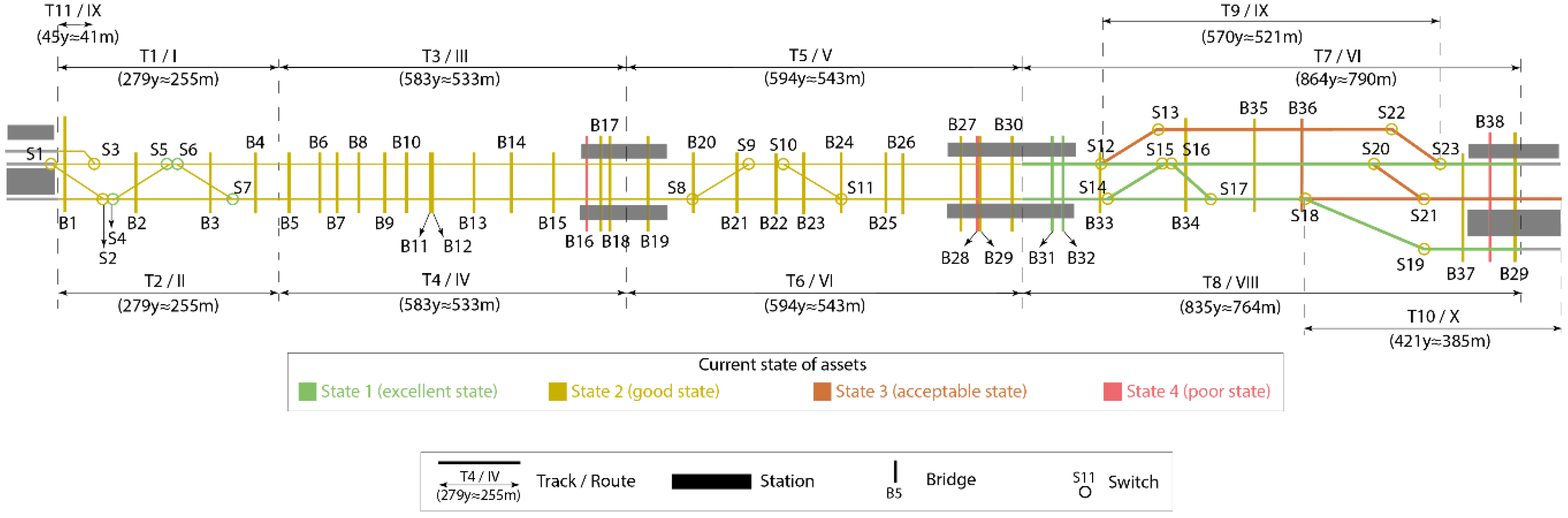
The approach presented in the paper is used to determine the optimal intervention program for an example network modelled after a 2200 m long line, which belongs to the Irish railway network that is located in Dublin, Ireland. All objects that were considered, their initial state, and the topological layout of the routes are shown in Figure 4. It consists of 5163 m of track divided into 11 objects, 23 switches, and 39 bridges with a total of 16,763 m² of bridge deck. A list with all objects, their extent, current state, affected route, and the risk that is related to each state is given in Appendix A (

Table A1. Track and switch objects.

Object	Extend	State	Affected Routes	Risk in State 1 [euros]	Risk in State 2 [euros]	Risk in State 3 [euros]	Risk in State 4 [euros]
T1	255 m	2	I	6277	62,769	188,306	1,077,730
T2	255 m	2	II	6277	62,769	188,306	1,077,730
T3	533 m	2	III	6535	65,348	196,043	1,321,163
T4	533 m	2	IV	6535	65,348	196,043	1,321,163
T5	543 m	2	V	6489	64,891	194,673	1,272,209
T6	543 m	2	VI	6489	64,891	194,673	1,272,209
T7	790 m	1	VII	6808	68,085	204,254	1,459,020
T8	764 m	1	VIII	6767	67,669	203,008	1,437,856
T9	521 m	3	IX	6230	62,305	186,914	1,220,734
T10	385 m	3	X	1142	11,415	34,246	114,154
T11	41 m	2	XI	506	5057	15,170	50,565
S1	-	2	I	8542	101,014	293,571	1,432,348
S2	-	2	II	8542	101,014	293,571	1,432,348
S3	-	2	I	8542	101,014	293,571	1,432,348
S4	-	1	II	8542	101,014	293,571	1,432,348
S5	-	1	I	8542	101,014	293,571	1,432,348
S6	-	1	I	8542	101,014	293,571	1,432,348
S7	-	1	II	8542	101,014	293,571	1,432,348
S8	-	2	VI	7092	78,982	218,675	1,153,207
S9	-	2	V	7092	78,982	218,675	1,153,207
S10	-	2	V	7092	78,982	218,675	1,153,207
S11	-	2	VI	7092	78,982	218,675	1,153,207
S12	-	2	VII	6808	75,470	208,123	1,129,964
S13	-	2	IX	6138	66,297	178,683	1,041,453
S14	-	2	VIII	6804	74,744	204,511	1,102,878
S15	-	2	VII	6804	74,744	204,511	1,102,878
S16	-	2	VII	6808	75,470	208,123	1,129,964
S17	-	2	VIII	6808	75,470	208,123	1,129,964
S18	-	2	VIII	6804	74,744	204,511	1,102,878
S19	-	2	VIII	6808	75,470	208,123	1,129,964
S20	-	2	VII	6808	75,470	208,123	1,129,964
S21	-	2	X	6535	71,162	193,198	1,070,946
S22	-	2	IX	6138	66,297	178,683	1,041,453
S23	-	2	VII	6806	75,107	206,317	1,116,421

and

Table A2. Bridge objects (part 1).

Object 1	Extend	State	Affected Routes	Risk in State 1 [euros]	Risk in State 2 [euros]	Risk in State 3 [euros]	Risk in State 4 [euros]
B1 (M)	720 m2	2	I, II, XI	0	27,340	521,126	51,272,150
B2 (C)	1130 m2	2	I, II	0	0	34,932	18,527,602
B3 (M)	470 m2	2	I, II	0	19,428	365,771	33,636,327
B4 (S)	320 m2	2	I, II	0	14,865	277,646	23,112,798
B5 (S)	372 m2	2	III, IV	0	0	15,914	6,110,853
B6 (S)	166 m2	2	III, IV	0	11,077	202,233	12,403,148
B7 (M)	166 m2	2	III, IV	0	0	9363	2,736,668
B8 (S)	350 m2	2	III, IV	0	17,622	326,172	25,327,612
B9 (S)	500 m2	2	III, IV	0	22,975	427,540	35,898,330
B10 (M)	250 m2	2	III, IV	0	14,053	258,594	18,280,467
B11 (S)	350 m2	2	III, IV	0	0	15,201	5,743,595
B12 (M)	1410 m2	2	III, IV	0	55,449	1,042,506	100,027,352
B13 (S)	500 m2	2	III, IV	0	22,975	427,540	35,898,330
B14 (M)	450 m2	2	III, IV	0	21,190	393,751	32,374,757
B15 (S)	400 m2	2	III, IV	0	19,406	359,962	28,851,185
B16 (S)	640 m2	4	III, IV	0	0	24,802	10,499,196
B17 (S)	230 m2	2	III, IV	0	13,605	252,644	16,959,412
B18 (M)	230 m2	2	III, IV	0	13,605	252,644	16,959,412
B19 (S)	960 m2	2	V, VI	0	0	34,988	15,745,743
B20 (S)	320 m2	2	V, VI	0	16,509	305,105	23,145,518
B21 (M)	600 m2	2	V, VI	0	0	23,088	9,841,172
B22 (M)	330 m2	2	V, VI	0	16,865	311,838	23,848,120
B23 (M)	460 m2	2	V, VI	0	0	18,648	7,546,107
B24 (S)	450 m2	2	V, VI	0	21,132	392,637	32,279,349
B25 (S)	650 m2	2	V, VI	0	0	24,673	10,660,838
B26 (S)	720 m2	2	V, VI	0	30,732	574,434	51,249,613
B27 (S)	270 m2	2	V, VI	0	14,997	279,005	19,720,881
B28 (S)	765 m2	4	V, VI	0	32,598	612,299	54,499,698
B29 (S)	192 m2	2	V, VI	0	7448	25,607	3,561,347
B30 (S)	110 m2	2	V, VI	0	0	7919	1,809,364
B31 (M)	160 m2	1	VII, VIII	0	6574	22,608	2,973,274
B32 (C)	240 m2	1	VII, VIII	0	8759	30,104	4,443,456
B33 (M)	345 m2	2	VII, VIII	0	0	11,763	5,602,012
B34 (M)	345 m2	2	VII, VIII, IX	0	0	11,806	5,602,088
B35 (M)	136 m2	2	VII, VIII, IX	0	0	7126	2,211,361
B36 (M)	425 m2	3	VII, VIII, IX	0	0	13,597	6,899,974
B37 (M)	187 m2	2	VII, VIII, X	0	0	8268	3,038,763
B38 (C)	187 m2	4	VII, VIII, X	0	0	8639	3,039,681
B39 (M)	255 m2	2	VII, VIII, X	0	0	10,161	4,142,885
B39 (M)	255 m2	2	VII, VIII, X	0	0	10,161	4,142,885

¹ The letter in bracket represents the bridge type as masonry (M), concrete (C), and steel (S).

). The risk related to an object being in a certain state was estimated using the risk assessment process presented in [32]. Infrastructure managers from Irish Rail have provided all cost and duration values used. The optimal intervention programs are determined for the situation where there is no budget limit and for the situation where there is a budget limitation of four million euros.

All interventions considered are listed in

Table 6. Interventions.

Category	Intervention 1	Type	Applied on State	Restored State	Cost	Duration
Track	Tamping	1	2	1	€7.5/m	457 m/h
	Ballast Cleaning	1	3	1	€1.9/m	119 m/h
	Track Renewal	1	1–4	1	€745.6/m	119 m/h
Switch	Manual Grinding	2	2	1	€10,000/asset	3 h/asset
	Welding	2	3	1	€10,000/asset	3 h/asset
	Renewal	2	4	1	€250,000/asset	36 h/asset
Bridge	Recoating	2	2	1	€250/m2	3.75 m2/h
	Strengthening (M)	2	3	1	€1000/m2	0.5 m2/h
	Strengthening (C)	2	3	1	€1000/m2	0.7 m2/h
	Strengthening (S)	2	3	1	€3000/m2	0.5 m2/h
	Renewal (M)	2	4	1	€8000/m2	72 h/asset
	Renewal (C)	2	4	1	€7500/m2	72 h/asset
	Renewal (S)	2	4	1	€5000/m2	72 h/asset

¹ The letter in brackets indicates the bridge type, i.e., masonry (M), concrete (C), and steel (S).

. Interventions of three different types can be executed on each object. The sharable portions of the costs for track and switch interventions, i.e., the economical dependencies, are 20% and 40%. To take advantage of these savings the objects have to be close to each other. For track, this means they are physically connected, e.g., T₁—T₃—T₅—T₇ and T₂—T₄—T₆—T₈. For switches, there are four groups S₁ to S₇, S₈ to S₁₁, S₁₂ to S₁₇, and S₁₈ to S₂₃.

The traffic states considered, with their unit cost per hour are listed in

Table 7. Traffic states (TS).

Closed Routes	Day (euro/h)	Weekend (euro/h)	Night (euro/h)
I	TS 1: 18,620	TS 15: 2437	TS 29: 0
II	TS 2: 18,620	TS 16: 2437	TS 30: 0
III	TS 3: 5008	TS 17: 882	TS 31: 0
IV	TS 4: 5008	TS 18: 882	TS 32: 0
V	TS 5: 6919	TS 19: 2199	TS 33: 0
VI	TS 6: 6919	TS 20: 2199	TS 34: 0
VII	TS 7: 4918	TS 21: 1420	TS 35: 0
VIII	TS 8: 4918	TS 22: 1420	TS 36: 0
IX	TS 9: 0	TS 23: 0	TS 37: 0
X	TS 10: 2767	TS 24: 880	TS 38: 0
XI	TS 11: 18,620	TS 25: 2437	TS 39: 0
I, II, III, IV, XI	TS 12: 41,671	TS 26: 13,235	TS 40: 0
V, VI	TS 13: 41,511	TS 27: 13,196	TS 41: 0
VII, VIII, IX, X	TS 14: 29,506	TS 28: 8520	TS 42: 0

. Each traffic state refers to a specific combination of a time window (e.g., day, weekend, and night) and the closed routes. For example, traffic state 1 refers to the closure of route I during weekdays, which leads to user costs of 18,620 euros per hour. Weekend and night windows are limited to 52 and 4 h of maximum work time, during which interventions can be executed. Interventions with a longer duration than the maximum work time of a time window cannot be executed during this time window and have to be executed during another time window. Track interventions are an exception to this rule, as they can be stopped anywhere and then resumed in the next time window at the same place.

This example has 3 × 10⁸² possible intervention programs, from which the optimal one is to be found. The model of the constrained network flow model consists of 986 nodes and 2015 edges, 2549 decision variables, 944 flow conservation constraints, and 735 side constraints. The constrained network flow model was programmed while using the software R [33].

5.2. Optimal Intervention Program with No Budget Constraint

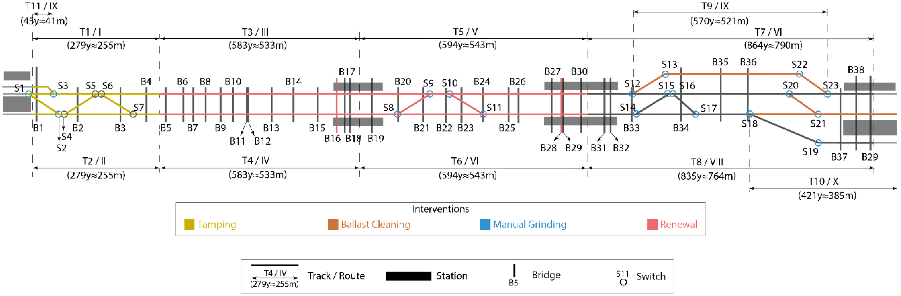
The optimal intervention program is shown in Figure 5 and

Table 8. Optimal intervention program determined using the network flow model.

Traffic State	Object	Intervention	Duration (h)	Owner Costs (Euros)	Risk Reduction (Euros)	4 M Budget
Day closure of	B16	Renewal	72.0	3,200,000	10,499,196	X
I, II, III, IV, XI	S1	Manual Grinding	3.0	10,000	92,472
	S2	Manual Grinding	3.0	6000	92,472
	S3	Manual Grinding	3.0	6000	92,472
Day closure of III	T3	Track Renewal	4.5	397,405	57,616	X
Day closure of IV	T4	Track Renewal	4.5	397,405	57,616	X
Day closure of	B28	Renewal	72.0	3,825,000	54,499,698
V, VI	S8	Manual Grinding	3.0	10,000	71,890
	S9	Manual Grinding	3.0	6000	71,890
	S10	Manual Grinding	3.0	6000	71,890
	S11	Manual Grinding	3.0	6000	71,890
Day closure of V	T5	Track Renewal	4.6	323,889	58,402
Day closure of VI	T6	Track Renewal	4.6	323,889	58,402
Weekend closure X	S21	Manual Grinding	3.0	10,000	64,627
Weekend closure IX	S22	Manual Grinding	3.0	6000	60,159
Night	T1	Tamping	0.6	1913	56,492	X
Night	T2	Tamping	0.6	1913	56,492	X
Night	T9	Ballast Cleaning	4.4	990	180,684	X
Night	T10	Ballast Cleaning	3.2	732	33,104
Night	T11	Tamping	0.1	308	4551	X
Night	S12	Manual Grinding	3.0	10,000	68,662
Night	S13	Manual Grinding	3.0	10,000	60,159
Night	S14	Manual Grinding	3.0	10,000	67,940
Night	S15	Manual Grinding	3.0	10,000	67,940
Night	S16	Manual Grinding	3.0	10,000	68,662
Night	S17	Manual Grinding	3.0	10,000	68,662
Night	S18	Manual Grinding	3.0	10,000	67,940
Night	S19	Manual Grinding	3.0	10,000	68,662
Night	S20	Manual Grinding	3.0	10,000	68,662
Night	S23	Manual Grinding	3.0	10,000	68,301

, along with information on the interventions to be executed, the amount of time required to execute them, their costs and their benefits in terms of risk reduction, and the traffic state in place during their execution. For example, bridge B₁₆ is renewed during the day for 72 h, while routes I, II, III, IV, and XI are closed. The owner intervention costs are 3.2 M euros and the benefit in terms of risk reduction is almost 10.5 M euros. Manual grinding interventions are executed during the same closure on the switches S₁, S₂, and S₃. Here, topological dependencies of the switches are exploited to reduce traffic disturbance. Traffic disturbance are also reduced by the parallel execution of the renewal intervention on bridge B₂ and the interventions on S₈, S₉, S₁₀, and S₁₁. Due to the execution of these switch interventions during the day, economical dependencies between the switches are exploited, which can be seen, for example, in the reduced costs of the intervention on S₉, S₁₀, and S₁₁. This results in a reduction of their costs by 40% from 10,000 to 6000 euros. Without the parallel execution of the bridge renewal interventions, which require the closing of the routes during the day, the cost reduction due to economical dependencies would not be enough to overcome the increased user costs. This is different for the combination of interventions on switches S₂₁ and S₂₂. There, the weekend execution does not lead to higher user costs than the achieved reduction in owner costs. The closure of the affected routes IX and X during the weekend costs the users 2640 euros, while the cost of the interventions that is saved due to their simultaneous execution is 4000 euros. The weekend execution for these two switches is, therefore, less expensive.

The traffic states required for executing the intervention program are given in

Table 9. Traffic states of the intervention program developed with the network flow model.

Traffic State	Closed Routes	Time Window	Duration (h) UL *	Cost (euro) UL *	Duration (h) L *	Cost (euro) L *
TS 3	III	Day	4.5	22,429	4.5	22,429
TS 4	IV	Day	4.5	22,429	4.5	22,429
TS 5	V	Day	4.6	31,570	-	-
TS 6	VI	Day	4.6	31,570	-	-
TS 12	I, II, III, IV, XI	Day	72.0	3,000,276	72.0	3,000,276
TS 13	V, VI	Day	72.0	2,988,789	-	-
TS 23	IX	Weekend	3.0	0	-	-
TS 24	X	Weekend	3.0	2639	-	-
TS 29–42	Different routes	Night	35.8	0	5.6	0

* Note: UL = unlimited situation, L = situation with a 4 M budget limitation.

. The traffic states involving night work are shown together, as they do not lead to user costs. The major user costs arise during the execution of interventions when traffic states 12 and 13 are in place. These traffic states require the closure of entire links, which increases user costs significantly over the closure of only single routes. Overall, the optimal intervention program when there is no budget constraint generates a net benefit of more than 52 million euros, i.e., a 67-million-euro benefit in terms of risk reduction, nine million euros of owner costs, and six million euros of user costs.

5.3. Optimal Intervention Program with Budget Constraint

The imposition of the budget constraint of 4 M euros, which is 47% of the money that is needed to execute all interventions to be executed without a budget limitation significantly reduces the number of interventions that can be executed. The interventions retained in the intervention program are indicated by the Xs in the last column of Table 8. The budget constraint, for example, results in the omission of the renewal of bridge B₂₈, which can only be executed together with the tracks T₅ and T₆ on the bridge, together resulting in 4.4 million euros (3.8 million for the bridge intervention and 0.6 million for the track intervention).

The net benefit of the intervention program with the budget constraint is approximately four million euros, i.e., a benefit of 11 million euros in terms of risk reduction, four million euros of owner costs, and three million euros of user costs. This is only 7.5% of the net benefit of the optimal intervention program without a budget limit. The large difference in net benefit is because the renewal intervention on bridge B₂₈ cannot be executed, and, therefore, the large benefits in terms of risk reduction resulting from this intervention could not be achieved.

6. Comparison

When there was no budget limit, the optimal intervention program determined while using the network flow model was compared with those determined using, (1) an exhaustive search approach and (2) a decision rule approach (

Table 10. Approaches used for comparison.

Approach	Intervention programs evaluated consisted of…	The 3 × 1082 possible programs were reduced…
exhaustive search	only interventions on objects with non-zero risk	to 4.5 × 1012 by grouping the objects with non-zero risks into independent object groups, using the possible economical and topological dependencies, and investigating the optimal intervention to be executed per group, one at a time.
decision rule	only interventions that result in the least possible traffic disturbance if they were executed alone	to 8.5 × 109 by eliminating many possible intervention combinations, which are either not feasible or are highly unlikely to be part of the optimal intervention program, while still being able to determine a near optimal intervention program.

). Both approaches were used to evaluate a subset of the total number of intervention programs since the 3 × 10⁸² possible programs could not be evaluated in a reasonable time. When there was a budget limit, the optimal intervention program that was determined using the network flow model was compared with the one determined using the decision rule approach. The exhaustive search approach could not be used, as a budget constraint imposed on interventions on all objects cannot be evaluated by investigating object groups one at a time.

The owner costs, user costs, risk reduction and the net benefit of the intervention programs determined using the three approaches are shown in

Table 11. Model comparison.

Parameter	Exhaustive Search UL *	Decision Rules UL *	Network Model UL *	Exhaustive Search L *	Decision Rules L *	Network Model L *
Owner costs [M euros]	8.6	8.8	8.6	-	4.0	4.0
User costs [M euros]	6.2	6.1	6.2	-	3.0	3.0
Risk reduction [M euros]	66.9	66.9	66.9	-	10.9	10.9
Net benefit [M euros]	52.1	52.0	52.1	-	3.9	3.9
Percentage of maximal net benefit	100%	99.8%	100%	-	7.5%	7.5%
Computation time	139 min	1 s	22 s	Approx. 1012 years	2 s	39 s

* Note: UL = unlimited situation, L = situation with a 4 M budget limitation.

. As the network flow model and the exhaustive search find the same optimal intervention program all numbers are the same. The decision rules approach yields a near optimal intervention program, but not the optimal one, therefore there are slight differences in the owner and user costs and the risk reduction. One of the differences in the intervention programs is that the interventions on switches S₂₁ and S₂₂ are executed during the night with the near optimal intervention program, whereas they are executed during the weekend with the optimal intervention program.

The computation time of each approach is also shown in Table 11. It can be seen that the network flow model determines the optimal intervention program considerably faster than the exhaustive search, but that it was not as fast as the decision rules. Of course, the even faster time that is required by the decision rule approach comes at the expense of lost optimality, or in other words lost net-benefit. At least for the example this does not seem to be worth it. One cannot, however, forget that there are many approximations that have gone into the development of the models of the railway network and the possible interventions. These assumptions reduce the significance of the difference between the theoretically optimal intervention program and the near optimal intervention program.

7. Summary and Conclusions

An approach to develop models to determine optimal intervention programs for railway infrastructure networks was presented, i.e., the one with the maximal difference between the benefit in terms of risk reduction and the costs to the owner and user of executing interventions. The developed models are network flow models formulated as mixed integer linear programs and are constructed as constrained minimum cost flow problems, which search for the flow with the minimum cost within a given network under the consideration of flow conservation in each node, budget constraint and constraints that ensure that the times required to execute multiple intervention simultaneously are correctly considered. It enables the consideration of

• economical dependencies (i.e., those between similar interventions allowing to reduce intervention costs),
• structural dependencies (i.e., those that mean that an intervention on one necessitates an intervention on another), and
• topological dependencies (i.e., those between objects in terms of the system functionality).

The approach was used to develop a model to determine the optimal intervention program for a network with 73 objects, i.e., 11 tracks, 23 switches, and 39 bridges. The optimal intervention program was determined for the situations with and without a budget limitation.

It was shown that the developed model was able to determine the optimal intervention program in much faster computational time than using an exhaustive search, even with a reduced search space. It was also shown that the developed model was slower, but more accurate than a more simplified approach that is based on straightforward decision rules. The significance of the trade-off between speed and accuracy depends on the accuracy of the underlying models of infrastructure and the possible interventions, as well as the amount of time available for analysis.

References

- Caetano, L.F.; Teixeira, P.F. Availability Approach to Optimizing Railway Track Renewal Operations. J. Transp. Eng. 2013, 139, 941–948. [Google Scholar] [CrossRef]
- Moreu, F.; Spencer, B.F., Jr.; Foutch, D.A.; Scola, S. Consequence-based management of railroad bridge networks. Struct. Infrastruct. Eng. 2016, 13, 273–286. [Google Scholar] [CrossRef]
- Zwanenburg, W.-J. Modeling Degradation Processes of Switches and Crossings for Maintenance and Renewal Planning on the Swiss Railway Network. Ph.D. Thesis, École Polytechnique Fédérale de Lausanne, Lausanne, Switzerland, 2009. [Google Scholar]
- Morant, A.; Larsson-Kraik, P.-O.; Kumar, U. Data-driven model for maintenance decision support: A case study of railway signalling systems. Proc. Inst. Mech. Eng. Part F J. Rail Rapid Transit 2014, 1–15. [Google Scholar] [CrossRef]
- Zhao, J.; Chan, A.H.C.; Burrow, M.P.N. A genetic-algorithm-based approach for scheduling the renewal of railway track components. Proc. Inst. Mech. Eng. Part F J. Rail Rapid Transit 2009, 223, 533–541. [Google Scholar] [CrossRef]
- Caetano, L.F.; Teixeira, P.F. Optimisation model to schedule railway track renewal operations: A life-cycle cost approach. Struct. Infrastruct. Eng. 2014, 2479, 1–13. [Google Scholar] [CrossRef]
- Fecarotti, C.; Andrews, J.D. Optimising strategy selection for the management of railway assets. In Proceedings of the Stephenson Conference: Research for Railways, London, UK, 25–27 April 2017. [Google Scholar]
- Furuya, A.; Madanat, S.M. Accounting for Network Effects in Railway Asset Management. J. Transp. Eng. 2013, 139. [Google Scholar] [CrossRef]
- Pargar, F. A mathematical model for scheduling preventive maintenance and renewal projects of infrastructures. In Safety and Reliability of Complex Engineered Systems; Podofillini, L., Sudret, B., Stojadinovic, B., Zio, E., Kröger, W., Eds.; Taylor & Francis Group: London, UK, 2015; pp. 993–1000. [Google Scholar]
- Den Hertog, D.; van Zante-de Fokkert, J.I.; Sjamaar, S.A.; Beusmans, R. Optimal working zone division for safe track maintenance in the Netherlands. Accid. Anal. Prev. 2005, 37, 890–893. [Google Scholar] [CrossRef] [PubMed]
- Jenema, A.R. An Optimization Model for a Train-Free-Period Planning for ProRail Based on the Maintenance Needs of the Dutch Railway Infrastructure. Master’s Thesis, Delft University of Technology Responsible, Delft, The Netherlands, 2011. [Google Scholar]
- Lethanh, N.; Adey, B.T. A real option approach to determine optimal intervention windows for multi-national rail corridors. Civ. Eng. Manag. 2016, 22, 38–46. [Google Scholar] [CrossRef]
- Van Zante-De Fokkert, J.I.; den Hertog, D.; van den Berg, F.J.; Verhoeven, J.H.M. The Netherlands schedules track maintenance to improve track workers’ safety. Interfaces 2007, 37, 133–142. [Google Scholar] [CrossRef]
- Budai-Balke, G. Operations Research Models for Scheduling Railway Infrastructure Maintenance. Ph.D. Thesis, Erasmus University, Rotterdam, The Netherlands, 2009. [Google Scholar]
- Pouryousef, H.; Teixeira, P.F.; Sussman, J. Track Maintenance Scheduling and its Interactions with Operations: Dedicated and Mixed High-speed Rail (HSR) Scenarios. In Proceedings of the 2010 Joint Rail Conference, Urbana, IL, USA, 27–29 April 2010; American Society of Mechanical Engineers: New York, NY, USA, 2010. [Google Scholar]
- Peng, F. Scheduling of Track Inspection and Maintenance Activities in Railroad Networks. Ph.D. Thesis, University of Illinois at Urbana-Champaign, Champaign, IL, USA, 2011. [Google Scholar]
- Burkhalter, M.; Martani, C.; Adey, B.T. Determination of Risk-Reducing Intervention Programs for Railway Lines and the Significance of Simplifications. J. Infrastruct. Syst. 2018, 24. [Google Scholar] [CrossRef]
- Hajdin, R.; Adey, B.T. Optimal worksites on highway networks subject to constraints. In Proceedings of the IFED, Lake Louise, AB, Canada, 26–29 April 2006. [Google Scholar]
- Eicher, C.; Lethanh, N.; Adey, B.T. A routing algorithm to construct candidate workzones with distance constraints. In Proceedings of the ICSC15: The Canadian Society for Civil Engineering 5th International/11th Construction Specialty Conference, Vancouver, BC, Canada, 8–10 June 2015; University of British Columbia: Vancouver, BC, Canada, 2015. [Google Scholar]
- Lethanh, N.; Adey, B.T.; Burkhalter, M. Determining an Optimal Set of Work Zones on Large Infrastructure Networks in a GIS Framework. J. Infrastruct. Syst. 2018, 24, 1–16. [Google Scholar] [CrossRef]
- Keizer, M.C.A.O.; Flapper, S.D.P.; Teunter, R.H. Condition-based maintenance policies for systems with multiple dependent components: A review. Eur. J. Oper. Res. 2017, 261, 405–420. [Google Scholar] [CrossRef]
- Papathanasiou, N.; Martani, C.; Adey, B.T. Risk Assessment process for railway network with focus on infrastructure objects. In Proceedings of the 1st Asian Conference on Railway Infrastructure and Transportation (ART 2016), At Jeju, Korea, 19–20 October 2016. [Google Scholar]
- Subramanian, A.; Brandstädt, A.; Nishizeki, T. Handbook of Graph Theory, Combinatorial Optimization, and Algorithms; CRC Press: Boca Raton, FL, USA, 2016. [Google Scholar]
- Paschos, V.T. Applications of Combinatorial Optimization, 2nd ed.; Wiley ISTE: Hoboken, NJ, USA, 2014; Volume 3. [Google Scholar]
- Bertsekas, D.P. Network Optimization: Continuous and Discrete Models; Athena Scientific: Belmont, MA, USA, 1998. [Google Scholar]
- Munkres, J. Algorithms for the Assignment and Transportation Problems. J. Soc. Ind. Appl. Math. 1957, 5, 32–38. [Google Scholar] [CrossRef] [Green Version]
- Bellman, R. On a Routing Problem. Q. Appl. Math. 1958, 16, 87–90. [Google Scholar] [CrossRef]
- Ford, L.; Fulkerson, D.R. Maximum Flow through a Network. Can. J. Math. 1956, 8, 399–404. [Google Scholar] [CrossRef]
- Truemper, K. On max flows with gains and pure min-cost flows. SIAM J. Appl. Math. 1977, 32, 450–456. [Google Scholar] [CrossRef]
- Ahuja, R.K.; Magnanti, T.L.; Orlin, J.B. Network Flows: Theory, Algorithms, and Applications; Prentice Hall: Upper Saddle River, NJ, USA, 1993. [Google Scholar]
- Beasley, J.E.; Christofides, N. An algorithm for the resource constrained shortest path problem. Networks 1989, 19, 379–394. [Google Scholar] [CrossRef]
- Papathanasiou, N.; Martani, C.; Adey, B.T. Risk Assessment Methodology; DESTination RAIL Deliverable D3.2; Swiss Federal Institute of Technology: Zurich, Switzerland, 2016. [Google Scholar]
- R Core Team. R: A Language and Environment for Statistical Computing; R Foundation for Statistical Computing: Vienna, Austria, 2016; Available online: https://www.r-project.org/ (accessed on 23 November 2018).
- Papathanasiou, N.; Adey, B.T.; Burkhalter, M. Risk Assessment Methodology; DESTination RAIL Deliverable D3.6; Swiss Federal Institute of Technology: Zurich, Switzerland, 2018. [Google Scholar]