Agent Based Model to Estimate Time to Restoration of Storm-Induced Power Outages


1
Department of Civil and Environmental Engineering, University of Connecticut, Storrs, CT 06269, USA
2
Department of Emergency Response, Eversource Energy, Berlin, CT 06037, USA
3
Department of Emergency Management, Jacksonville State University, Jacksonville, AL 36265, USA
*
Author to whom correspondence should be addressed.
Infrastructures 2018, 3(3), 33; https://0-doi-org.brum.beds.ac.uk/10.3390/infrastructures3030033
Submission received: 12 July 2018
/
Revised: 26 August 2018
/
Accepted: 27 August 2018
/
Published: 31 August 2018
Abstract
:Extreme weather can cause severe damage and widespread power outages across utility service areas. The restoration process can be long and costly and emergency managers may have limited computational resources to optimize the restoration process. This study takes an agent based modeling (ABM) approach to optimize the utility storm recovery process in Connecticut. The ABM is able to replicate past storm recoveries and can test future case scenarios. We found that parameters such as the number of outages, repair time range and the number of utility crews working can substantially impact the estimated time to restoration (ETR). Other parameters such as crew starting locations and travel speeds had comparatively minor impacts on the ETR. The ABM can be used to train new emergency managers as well as test strategies for storm restoration optimization.
1. Introduction
Electric utility consumers rely on consistent access to electricity for daily activities. Extreme weather can cause power outages lasting for long durations and cost US consumers $20 to $55 billion a year [1]. In the United States, utilities are required to report events that cause power loss to at least 50,000 customers to the North American Electric Reliability Corporation. In 2017 there were 147 total outage events and 77 of those were caused by extreme weather. These 77 weather-related events affected about 19 million utility customers [2]. With occurrences of extreme weather increasing, there is a potential for increases in extended power outages. For example, climate change is likely to increase the intensity and frequency of hurricanes along the eastern seaboard and the frequency of extreme rainfall events [3]. Climate change is highly likely to increase risks from heat stress, storms and extreme precipitation, inland and coastal flooding, sea level rise and storm surge [3].
A system restoration solution must be feasible, provide as much service to customers as possible, be implemented as quickly as possible and not cause further damage to the system [4]. Utility companies tend to have their own approach to prioritizing the restoration of their customers but currently there are few resources or analytical tools available to aid in the decision-making process. Utilities rely on past experience from emergency managers in crew allocation decisions. For example, utilities have limited crews available and therefore there is a limit on the number of outages they can repair per day. When the number of outages is high enough that restoration will take many days, utilities may turn to mutual assistance groups to decrease the time to restoration. The mutual assistance program allows utilities to allocate unused crews to areas that were more severely affected by a storm. However, some storms are large and widespread and mutual assistance crews must travel large distances to provide the necessary support, costing utilities a significant amount of money and delays in restoration.
Several models have been developed to study storm restoration. The Institute of Electrical and Electronics Engineers (IEEE) created a model to test the organizational system of utility crews by considering the boundaries of service territories and districts and then considering crew assignments within those districts [5]. The IEEE model was mostly used to determine the optimal territory configuration and the crew assignments within those territories and was not used for recovery methods, leaving utility companies to continue to base their strategies off past experiences rather than specific models. Nateghi et al. (2011) developed several regression models to estimate the outage duration for individual outages. This model includes parameters specific to the power system, along with weather and geological parameters and were applied to outages in Hurricane Ivan. They determined which variables contributed negatively or positively to the outage duration time and noted that the number of available crews is a very important factor in determining the length of the outage but was not incorporated in the model [6]. Another model developed by Wanik et al. (2018) incorporated the number of crews working and customer variables (the peak customers affected). Data was used from Storm Irene, a 2011 October Nor’easter and Hurricane Sandy to develop an outage repair rate based off the known number of outages fixed and the number of crews working to develop an ETR model [7]. Liu et al. [8] proposed an expert system approach. This approach was justified because they argued that the restoration process involves logical reasoning. The expert system approach determines an optimal order of outage repairs for general system restoration or to minimize power losses. This approach is based on the utility system itself and not the social system of the crews. System restoration is difficult to solve using mathematical programming because of its combinatorial nature. Ingram [9] modified an existing optimization model used by Atlantic Electric to determine the best location to stage crews. Ingram states that the model can also be used to justify restoration decisions to state regulators. The use of a model can be a consistent tool in cases where past experience of decision-making personnel is limited due to infrequent events.
An alternate approach can be to describe electric utility grids as complex systems. Electric distribution systems have a large number of elements, which makes modeling these systems very intricate [4]. More specifically, power outage repairs have many factors that need to be considered when estimating system restoration. These include the number of outages, the location of outages, storm length and repair times, which can all determine whether it is beneficial for a utility company to call in mutual assistance. There is quite a bit of complexity when assessing storm repair times.
Other factors that need to be considered includes how the crews are dispatched, which was not included in prior research articles. Crews can be dispatched from centralized Area Work Centers or dispersed randomly throughout the state. There are a number of basic questions that should be asked to optimize storm recovery; such as (a) will repairing outages from most to least customers affected without regards to travel distance be more beneficial?; (b) would it be better for a crew to go to the nearest outage regardless of how many customers are affected?; (c) should a crew seek outages with the most customers affected within a given radius of the nearest outage?
Agent based modeling (ABM) is a modeling technique comprised of a set of agents that are given defined rules and allowed to operate in a given environment [10]. They have been used to study evacuation routes after tsunamis [11], model crowdsourcing systems [12], risk-based flood incident management [13], coupled human and natural systems [14] and to develop an electric power and communication synchronizing simulator [15]. ABMs can be used to model complex systems, such as human-environment interactions. The model is allowed to run on its own and is studied for emergent behavior that may not be expected prior to utilizing the model. ABMs provide a platform to implement an environment with its features, to forecast and explore future scenarios, experiment with possible alternative decisions, set different values for decision variables and analyze the effects of these changes [16]. Agents change the environment around them by following the simple rules they are assigned. Agents must interact with their environment, be independent, have social ability, be reactive and be proactive [17]. The goal of the project is to develop a working ABM to simulate power outage restoration that could be used to determine the optimal repair strategy. Unlike previous work, the ABM could be used to better estimate a time to complete restoration. The model could be used as a decision-making mechanism or as a training tool for new emergency managers. The ABM incorporates real decisions for users to make, as well as accurately simulating the crew’s response to those decisions and is validated with five historic storms.
2. Methods
2.1. Model Setup
In this paper, the ABM contains five different agent classes: utility crews, roads, power outages, area work centers and utility lines. The characteristics for each of these classes were drawn from existing datasets. The road dataset for Connecticut was obtained from the University of Connecticut Map and Geographic Information Center [18]. The points from the data file were uploaded into NetLogo software [10] and connected via links to make connected roadways for the crews to follow. The utility line dataset was obtained from Eversource and imported into the model similarly to the road system using links. The area work centers (AWC) are centralized locations around the state of Connecticut from where distribution equipment is stockpiled and crews are dispatched. These three agent sets are consistent in all model runs. The power outages were integrated into the model in one of two ways. For past storms, the power outage locations are known and are loaded into the model. If the user is interested in a what-if scenario, the power outages can be randomized and the model places them anywhere along the road system within the state of Connecticut.
To optimize model performance, the outages were geolocated to the nearest roadway. This allows the utility crew agents to move along the road network to the outage. The utility crews were treated as independent agents and have rules assigned to them. Each crew operated independently but they may survey nearby crews in order to make decisions about where to go next. It is important to note that the model does not take power system dynamics and switching into account as outages are treated as individual events that can be repaired by a single crew.
When the model begins, the roads and power lines are loaded first, followed by the outages and then the AWCs. All of these except the outages were the same for every model run. The number of outages and locations can vary and were determined by the user prior to model setup. In the ABM one “tick” is equal to the time interval set by the user. The range can be varied from 5 to 15 min, depending on how granular the output should be. All runs for this study were completed with a 15-min interval. The travel speed for all roads in Connecticut were set equal as determined by the user and could be varied for each model run from 25 to 50 mph. For each time step, a crew moves the distance equal to the travel speed times the time interval, unless the crew was on break or at their assigned outages.
In this application, the ABM uses a distributed approach because the agents are equipped with self-organizing rules to reach the end goal of system restoration [14]. The agents in the ABM are independent because they act without direct control of a human or other device. They are social because they communicate the outage they chose and their location with other agents. They are reactive to their environment because they repair damaged outages and ignore repaired outages. Lastly, the agents are proactive because the overall goal is to repair the outages according to the assigned rules.
The user has multiple options for the rules assigned to the crews. First, the crews can start at AWCs or they can be randomly placed across the State of Connecticut. The number of available crews can be set by the user, as well as any mutual assistance crews and the time until their arrival from out of state. During storms with restoration times over 24 h, crews will be required to take breaks. The ABM utilizes a percentage approach. During an eight hour shift a user defined percentage of crews will be working. This allows the user to set an overall number of crews but change the percent working during different eight hour shifts to simulate crews working and on their breaks. This approach allows the user to differentiate between day, evening and night hours. It also provides a way to allow some crews to keep working while others have stopped, instead of all crews working and on break during the same time period. Using past storm data, the total number of crews for a storm was calculated by adding the number of working crews and crews on break. Then a percentage of the total crews on break was calculated from this total. One storm may take several days and the average percentage for each of these time periods was calculated. For simulated storms, the average break period of eight hours from the validation storms was used to determine the overall percentage of crews working or on break during each time period.
2.2. Model Run
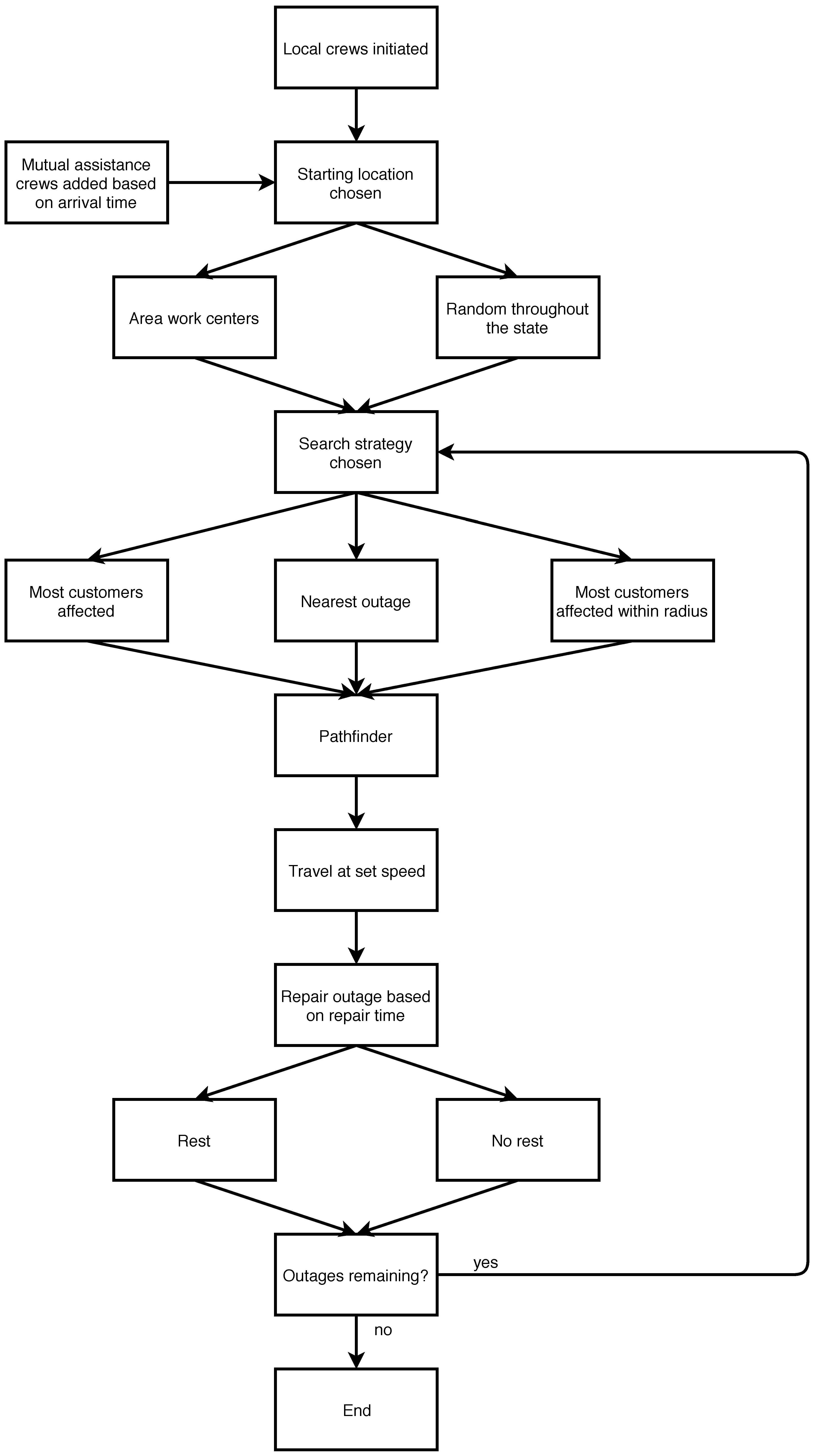
Once the ABM has gone through the setup process, the model follows an ordered procedure for each tick. First, all of the crews determine the next outage they will go to if they do not already have an outage assigned to them. The options are either the (i) nearest outage, (ii) the outage with the most customers affected, (iii) finding the nearest outage then setting a radius around it and within that radius choosing the outage with the most customers affected, (iv) outage with the fastest repair time, (v) finding the nearest outage then setting a radius around it and within that radius choosing the outage with the fastest repair time, or (vi) outage with the fastest repair time and most customers affected. The third option (which will be simplified as “nearest within radius”) simulates when crews can travel a little further in order to have a greater impact on the number of customers still without power. Once the crew determines its next outage, it changes the outage it found from “not taken” to “taken.” In the case where there are more crews than outages, crews may call off another crew if the crew without an assigned outage is closer to the unrepaired outage. After a crew determines the outage it will travel to, Dijkstra’s routing algorithm is used to determine the shortest distance for the crew to travel along the road network to their assigned outage. The algorithm factors in the number and length of links to determine the optimal path. Dijkstra’s algorithm will determine the optimal path by finding the combination of the least amount of links to travel and the overall shortest path [19]. Dijkstra’s algorithm has been used to model travelers taking public transportation and driving a vehicle [20]. However, Dijkstra’s algorithm does not take power flow into consideration to prevent crews from working too close. Over a series of ticks, the crew will travel at a user defined speed until it reaches its outage. During the travel time, the outage will remain as “taken” and “unrepaired.” The crew will stay at the outage and “work” for the user defined repair time assigned to the outage during the setup. Once the crew finishes the repair, it will update the outage to “repaired” and check if the crew is next to take a break. If so, the crew’s break time will start and they will remain on break at their current location for the next eight hours or the equivalent of one shift. Once the break is over, the crew will select a new outage as long as there are still “unrepaired” outages. If all of the outages are set as “taken” but do not yet have a crew there working, a crew can call off another crew if they are closer. This simulates the end of a storm with utility companies trying to finish the remaining outages as quickly as possible. The model stops once no more crews are working and all of the outages have been repaired. Figure 1 illustrates the decisions made by the model.
As shown in Figure 1, mutual assistance crews may be arriving throughout the storm. At each tick, the model does a check to see if any mutual assistance crews will be arriving. If so, the model will sprout new crews. Just like the initial crews, the mutual assistance crews will either start at AWCs or randomly across the state depending on the user chosen parameters. Once initiated, the mutual assistance crews operate identical to the original crews. Mutual assistance crews keep track of their travel time, their work time and their travel time back to where they started from. The model assumes mutual assistance crews begin traveling as the model starts running. Therefore, mutual assistance crews can keep track of how long they traveled, the amount of time they worked and include their travel time back home. If the crew will be assisting a different utility after completing their work in Connecticut, the travel time back to their home state will not be included. The total time the mutual assistance crew was traveling and working for the utility is used to calculate the cost of their aid. The cost of each crew is added together and the total cost of mutual assistance is displayed to the user at the completion of the model run. The hourly rate of the mutual assistance crews can be varied by the user.
2.3. Model Validation
Model validation was completed utilizing past storm data and tested using different combinations of parameters. These data included outage locations, number of customers affected and number of crews working. Since the nature of storm damage is different for each storm, outage repair times were varied uniformly between lower and upper limits to optimize the fit compared to past storm restoration curves. Moreover, the crew starting locations (area work center or random) and search strategy (nearest, most customers affected, most customers affected within a radius of the nearest outage, fastest repair time, fastest repair time within a radius and fastest repair time with most customers affected) were also varied to optimize the validation. Model fits were assessed using R2, mean absolute error (MAE) and standard deviation.
3. Results and Discussion
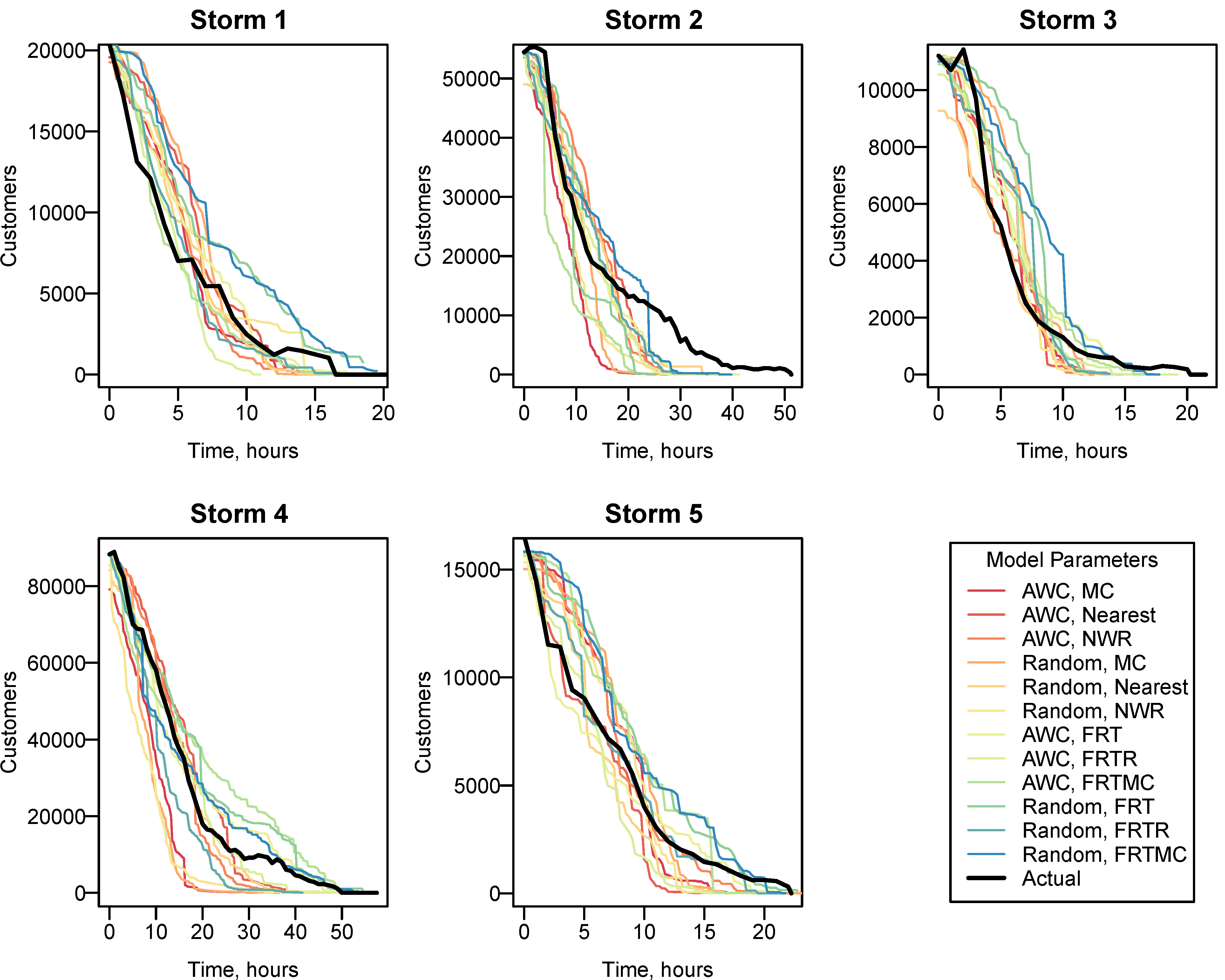
The first step in model validation was to compare modeled versus the actual restoration curves obtained from the utility company. With multiple input parameters for the model, the first task was running the model for all combinations of search strategies. The number of crews working for each storm was known from information obtained from the utility company, along with outage locations and number of customers affected at each outage, as shown in Table 1. The data obtained for the number of crews varied over time. Crews are moved to different areas throughout a storm, which results in fluctuations of the total number of crews on duty. In the model, the percent of crews working during a given day, evening or night shift corresponds to data from the actual storm. A summary of the total number of crews and the percentage working during day, evening and night hours is shown in Table 1. Travel speeds were set to 25 miles per hour and the repair time range was set as indicated in Table 1 with a uniform distribution. Storm repair curves from five different storms are shown in Figure 2. Outage repair time ranges were optimized for each storm and are shown in Table 1 and Table 2. While all repair curves showed similar large-scale behavior, there were significant differences between combinations of search strategies and starting location. However, neither the starting location nor the search strategy showed consistent trends (Figure 2).
Table 2 includes the R2 value, mean absolute error (MAE) and standard deviation for the top three strategies of each storm shown in Figure 2. Table S1 includes all strategies of each storm. Storm 1 was best fit with crews starting at area work centers and searching for the outage with the fastest repair time and the most customers affected. Storms 2 and 3 were best fit with crews starting at area work centers and searching for the outage with the fastest repair time. Both Storms 4 and 5 were best fit with crews searching for the fastest repair time within a radius of the nearest outage but Storm 4 favored crews starting at area work centers while Storm 5 favored random crew starting locations. Optimized fits had R2 values ranging from 0.91 to 0.99, indicating adequate fits for all scenarios.
An analysis of the residuals (Figure 3) indicates that they tend to be positive in the beginning of storms but this is not always the case. Storms 2 and 4 were larger in size and had negative residuals in the beginning meaning that they overestimated customers restored early in the storm. The early storm underestimates seen in Storms 1, 3 and 5 could be due to the fact that the model does not include priority locations such as hospitals. Utilities are aware of outages that impact the most customers and will restore these points first. Moreover, at the end of storms, there is typically a long tail representing outages that are difficult and time-consuming to repair and single service outages. The residuals in Figure 3 have been normalized to the maximum number of customers affected per storm. The residuals were biased because they were not randomly positive and negative. Storms 1, 3 and 5 had the lowest residuals. Storms 2 and 4 have larger residuals and as seen in Figure 3. In all cases, the residual values decrease towards zero at the end of storm recoveries.
Each storm is different in the damage it produces and therefore the length of time that repairs take on average. It is difficult to know the average repair time range of a storm before the storm occurs. As shown in Figure 2 and Table 2, each storm is fit with a different repair time range. These ranges were determined using the data in Figure 4 and Table 3. Table 3 includes the top three R2 value, mean absolute error (MAE) and standard deviation for each storm shown in Figure 4. R2 values were all >0.93. Table S2 includes all storms and all strategies. In these simulations, crews started at random locations and searched for the nearest outage. In all cases, as the repair time range was increased starting at one hour, the MAE decreases as the R2 value increases until the combination of highest R2 and lowest MAE is reached. Storm 1 appeared to match well with a lower maximum repair time early in the restoration but a longer repair time later on. Storms 2 and 4 best fit to a 13 h maximum repair time and were both larger storms in this data set with 1399 and 2056 outages respectively. Storms 1 and 5 were similar in size (657 and 661 outages) but the best fitting repair time was 7 h for Storm 1 and 11 h for Storm 5. The repair time range that best fits each storm depends on more than storm size alone. Storms 1, 3 and 5 had similar number of total crews working with 201, 212 and 190, respectively. Storm 2 had 365 and Storm 4 had 392. The larger storms had more crews working, yet still had the longer repair time range.
3.1. Model Sensitivity
With a reasonably validated model, we next tested the sensitivity of the model to outage locations. The model was run first using the known outage locations of historic storms. It was run again using the same number of outages but randomly placed across the State of Connecticut. For consistency, the average repair time range of 1 to 10 h will be used for all subsequent What-If scenarios. As seen in Figure 5, the two outage location options produced nearly identical results. This means that knowledge of actual outage locations is not necessary to reproduce accurate ETR curves. The model showed little sensitivity to travel speed, so the time lost to travel is negligible. Therefore, the location would have little impact on the ETR because any change due to travel distance is minor. For all storm simulations, outages will be randomly located within the state.
Tests were conducted to determine the sensitivity of the model to parameter changes. A small storm in these tests is characterized as having 1000 outages, large storms have 5000 outages and extreme storms have 15,000 outages. The number of customers affected per outage was determined by using an average from the five validation storms.
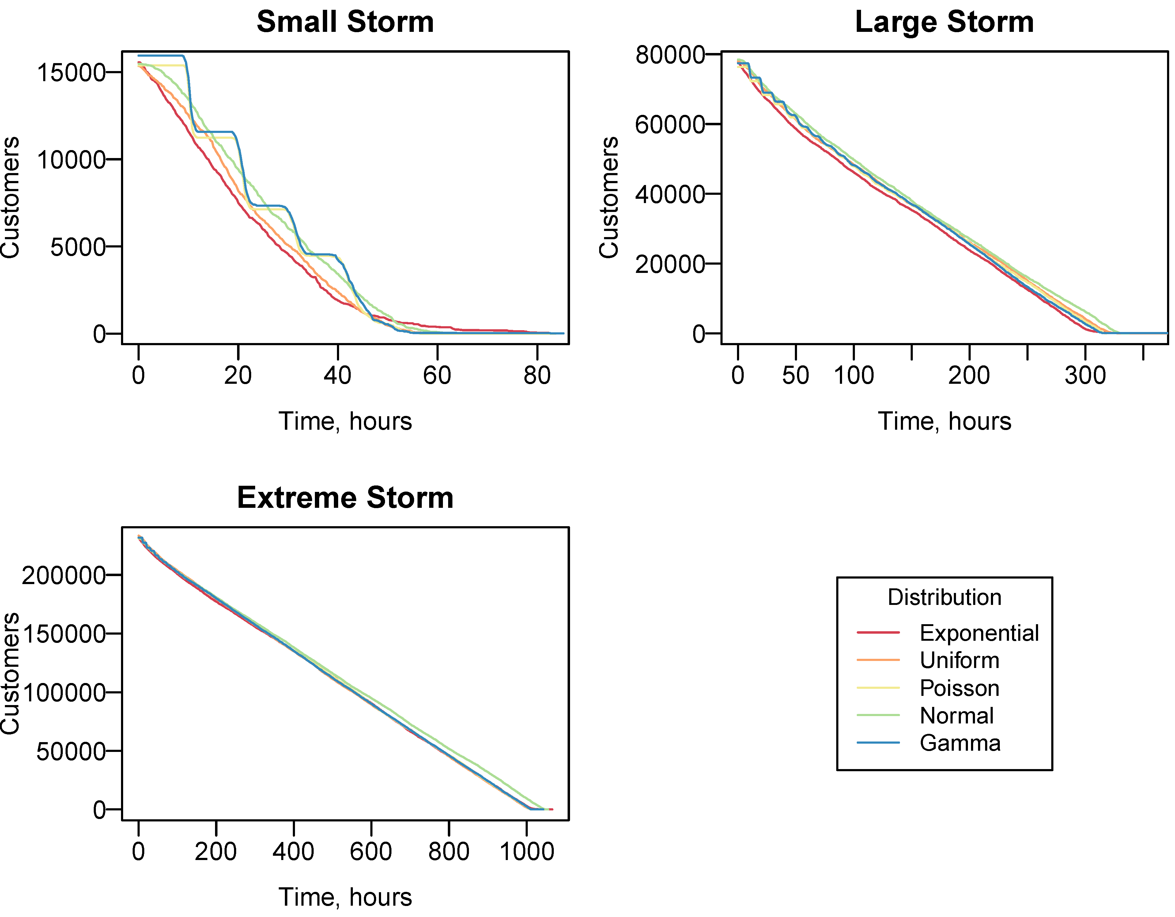
The model was tested for sensitivity to the outage repair time distribution. Previously shown results used a uniform outage repair time from 1 h until the chosen maximum repair time. However, it was unclear if different repair time distributions would lead to different overall restoration times. Storm characteristics can influence the nature of the damage caused and therefore the repair time distributions. Tested distributions included uniform, normal, exponential, gamma and Poisson and are detailed in Table 4. Figure 6 shows that the distribution of outage repair times has minor impacts on the final restoration time. As seen in the small storm, a gamma and Poisson distribution tends to produce a step-like restoration curve. Gamma distributions usually fit best with data with large standard deviation but the relatively low mean of the chosen repair times limits a large range. In the case a negative repair time was chosen, the model picks a new repair time. When all outages have the same repair time a step-like curve is produced because the crews arrive to their outage at similar times and are all working for the same duration. These steps become less defined over the course of the restoration process.
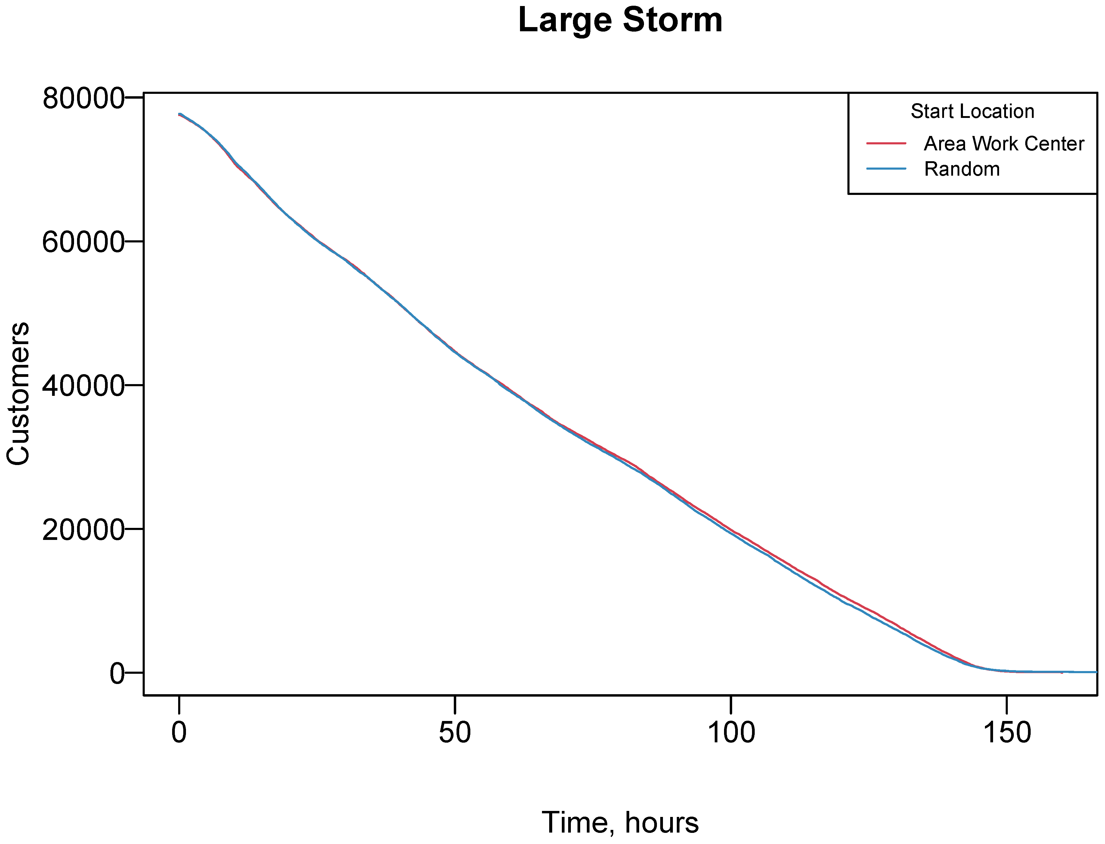
The next test compared the initial starting location of work crews for each size storm. At the beginning of the storm, crews could start at either area work centers or random locations. For this test crews would search for the nearest outage. Travel speed was set to 25 miles per hour, the repair time range was 1 to 10 h and 272 crews were working (the average number from the validated storms). Figure 7 shows that there was little difference between the two starting location options. All future storms will be run with crews starting at area work centers, which is more realistic.
As seen towards the end of the storm in Figure 7, some of the model runs can result in a long tail until complete restoration. This occurs when the last few outages have long repair times and when there are many single service outages. These long tails also can occur as difficult or hard to reach repairs are often left until the end. To highlight the major scenario differences, all ETR curves will be cropped when the number of customers remaining without power was no more than 20 for the small storm and 100 for the large and extreme storms. Figures S1–S3 for small and extreme storms can be found in the Supplementary Materials.
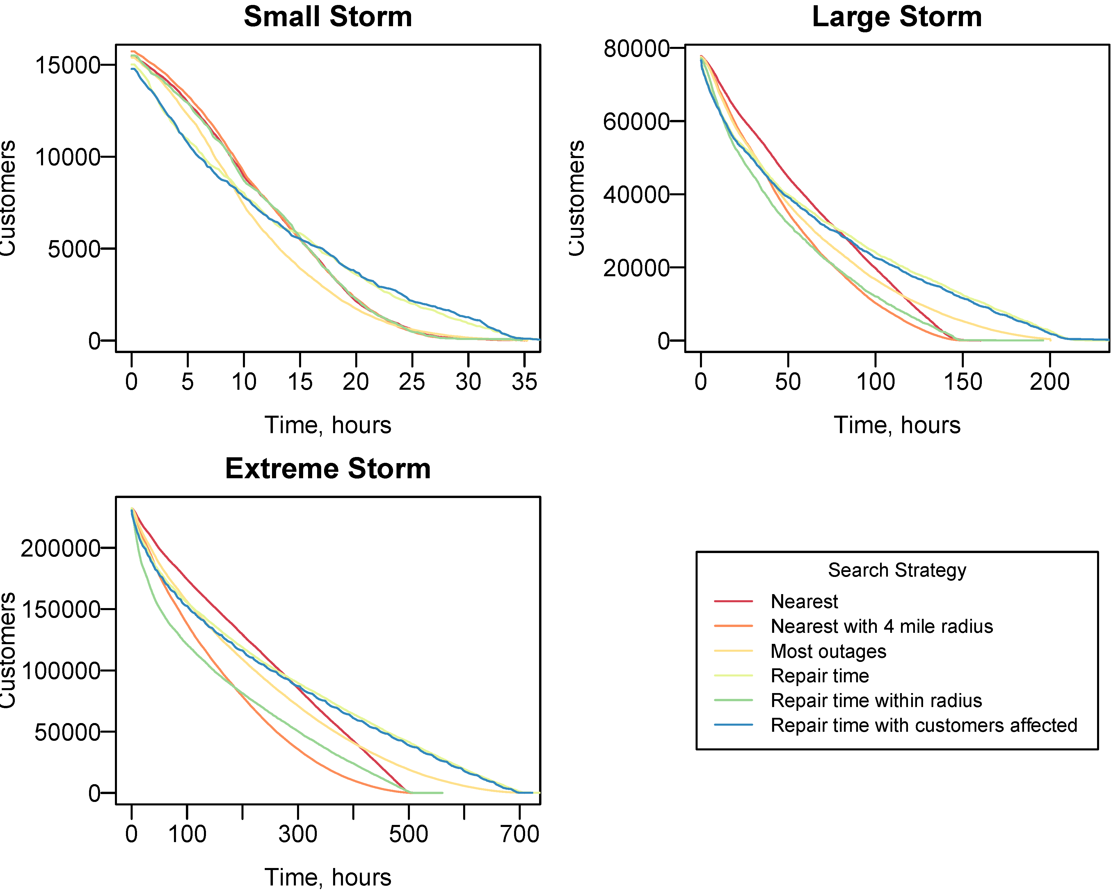
Next, the crew search strategy was varied between nearest outage, the outage with the most customers affected within a radius of the nearest outage (nearest within radius), the outage with the most customers affected, the outage with the fastest repair time, the outage with the fastest repair time within a radius of the nearest outage and the outage with the fastest repair time and most customers affected. All of the parameters were kept the same as previously described and crews started at area work centers. The radius was set to four miles for the nearest within radius and fastest within radius search options. Figure 8 shows some sensitivity to search strategy, especially in the large and extreme storms. For the small storm, there was little difference between the nearest outage, nearest with radius and fastest repair time. The most customers affected option performed better in the beginning but a longer tail at the end lengthened the final ETR. The large storm shows a bigger difference between the nearest outage and nearest with radius options. However, the nearest within radius performed similar to the most outages option in the beginning but ended faster than most outages. The nearest and nearest within radius search strategies had similar ETRs for the large storm but nearest within radius always had less customers still without power than nearest. The biggest differences between search options came in the extreme storm situation. The nearest within radius option performed best throughout the run. In the beginning of the simulation most outages performed between nearest within radius option and nearest outage, until about the 400-h point. After the 400-h mark, the most outages option reduced the number of customers affected most slowly. The nearest within radius option reduced the number of customers affected the fastest and had an ETR closest to the nearest search strategy. In both the large and extreme storms, the search strategies using repair times have similar impacts on the ETR curves. Both fastest repair time and fastest with most customers have the longest final ETR. The fastest within radius performs the best in the beginning of the storm but then has a final ETR similar to the nearest and nearest with radius strategies. The final ETR for each search strategy and storm size can be seen in Table 5.
As previously stated, a four-mile radius was used for the nearest within-radius search option. Next, this radius was varied from one mile to five miles. Figure 9 shows that the impact of the change in radius depends on the storm size and Table 6 shows the time to restoration in days for each storm size and radius. The small storm was not sensitive to the radius, which confirms from Figure 8 that there was little performance difference between the nearest outage option and nearest with radius option. However, the large and extreme storms were both sensitive to search radius. In both cases, a larger radius reduced the customers without power the quickest. However, the five-mile radius did have the longest tail in both the large and extreme storm.
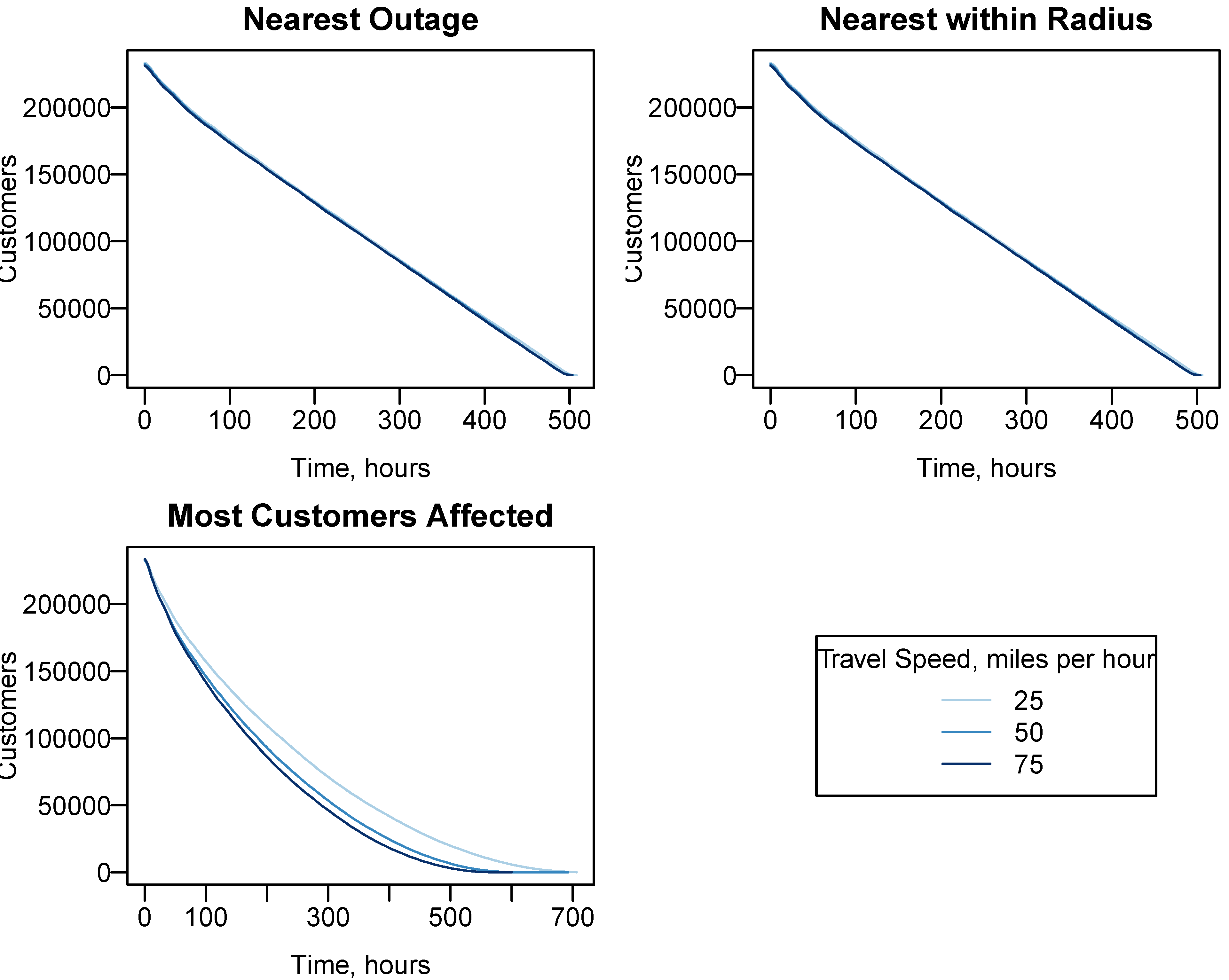
Next the model was tested for sensitivity to travel speed. The crew travel speed has little impact on the ETR, as shown in Figure 10 for the large storms with 5000 outages and with the nearest outage and nearest within radius search strategy. However, there are slight differences in the 25 mph, 50 mph and 75 mph speeds for most outages search strategy. Repeating for the small and extreme storms yielded similar result. The small storm was not run for the nearest with radius strategy because previous tests showed it did not vary from the nearest strategy. Figures S1–S3 for the small and extreme storm can be seen in the Supplementary Materials. The biggest difference for all three storms was between the 25 mph and 50 mph speeds for the most outages search strategy. Increasing from 50 mph to 75 mph further reduced the ETR but not as much as 25 to 50 mph. For all three storms, the different travel speeds did not significantly alter the final restoration time.
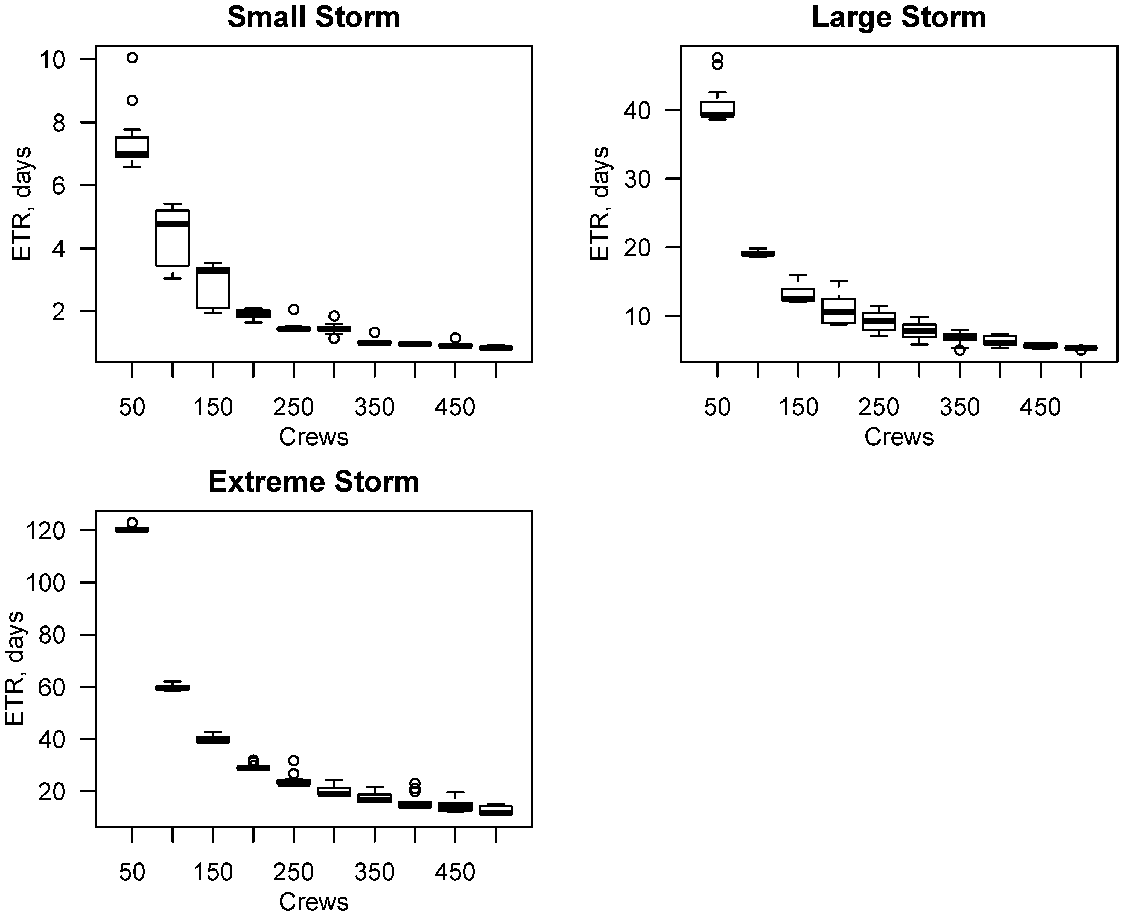
The next test varied the number of crews, as shown in Figure 11. For each storm size, initially increasing the number of crews creates a decrease in the ETR. However, there is a threshold where bringing in more crews will have less of an impact on the ETR. For the small storm, this occurred around 250 crews and for the extreme storm it was somewhere between 400 to 450 crews. Table 7 shows the time to restoration of each storm size based on number of crews from Figure 11.
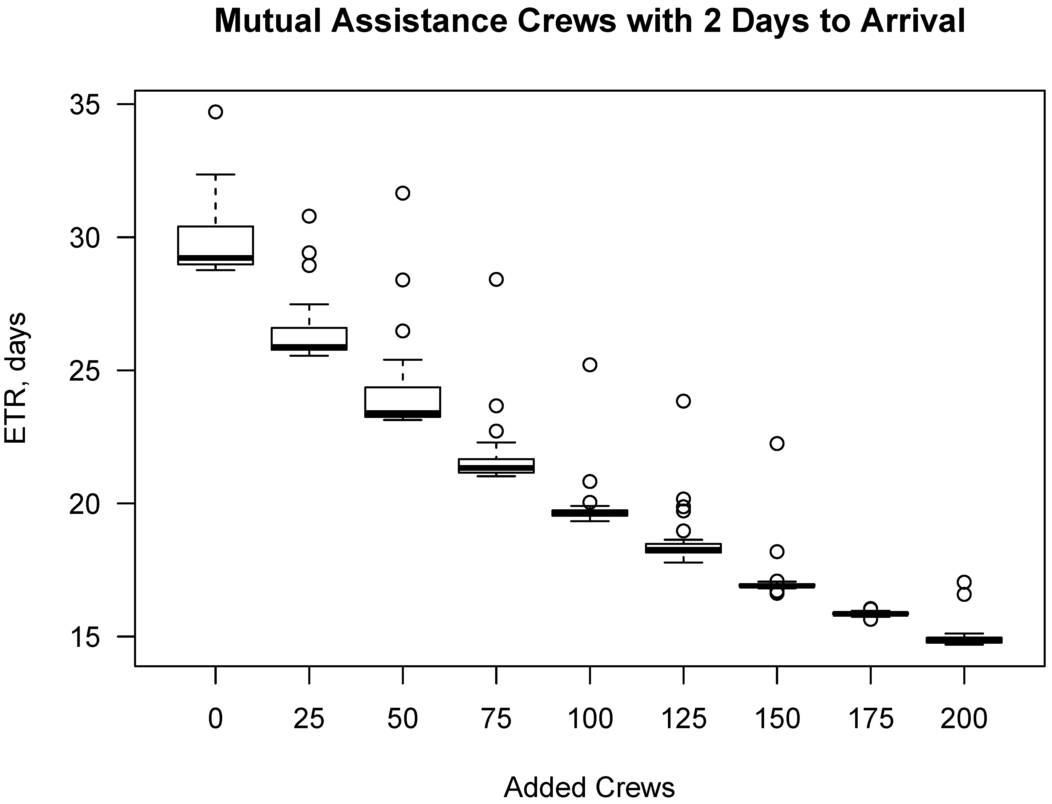
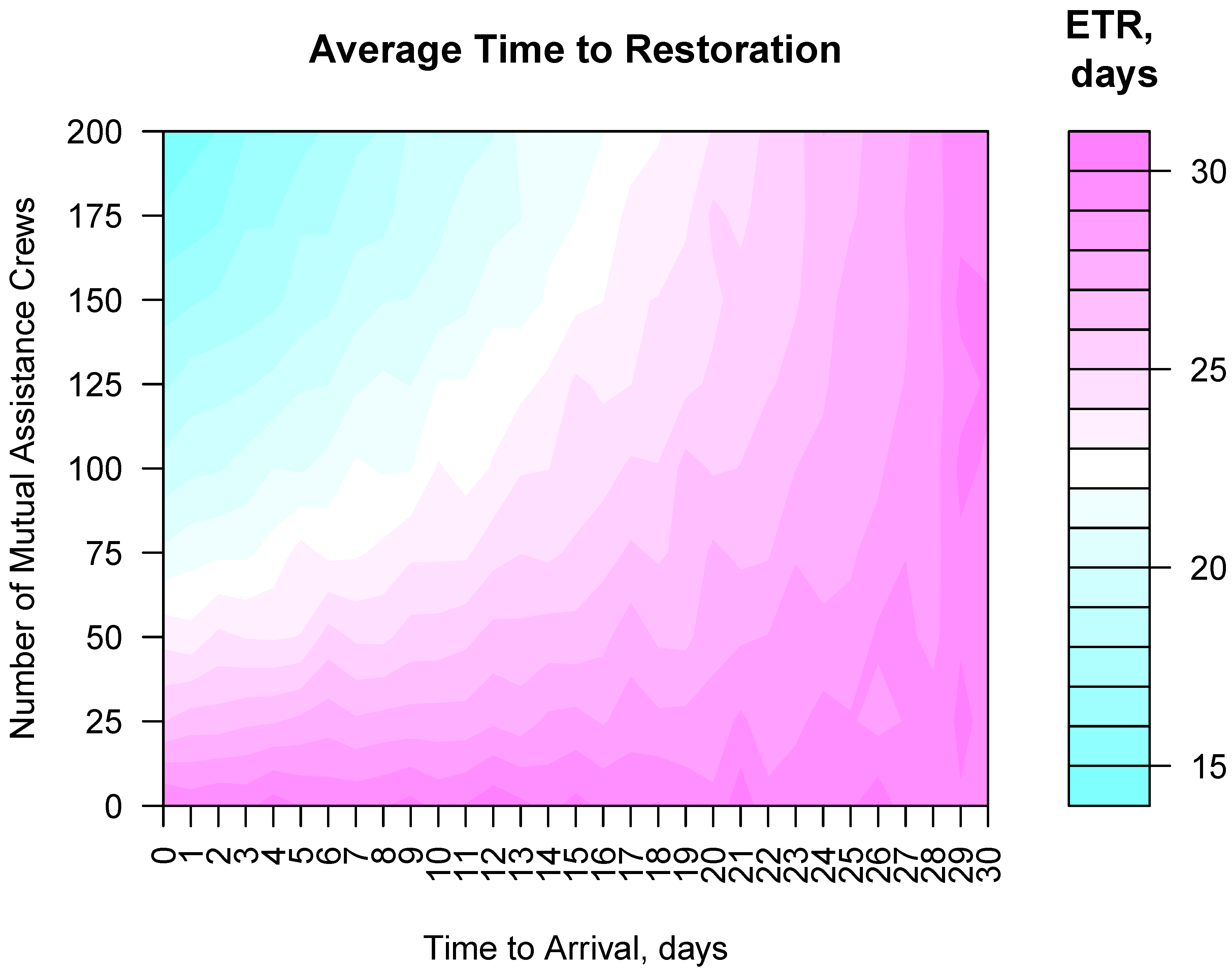
As previously mentioned, for storms with a lot of predicted outages, utility companies will call in mutual assistance crews to aid in the recovery process. This test looked at the impact on the ETR of bringing in mutual assistance crews at different times throughout the storm. First, only the time to arrival of 150 mutual crews added to 200 initial crews was varied as shown in Figure 12 for the extreme storm only. The ETR increases with increasing time for arrival. Next, the number of crews added to 200 initial crews with a two-day arrival was varied as shown in Figure 13. The ETR decreases with increasing number of added crews. Lastly, both the number of mutual assistance crews and the time to arrival was varied as shown in Figure 14. Also, as expected, the more crews and faster time to arrival decreased the ETR while less crews and longer time to arrival increased the ETR. There was also a point where calling in more crews that would take longer to get there made less of an impact in the ETR than calling in less crews that could arrive sooner. Towards the end of a storm there are less outages to repair. If a large number of mutual assistance crews arrive later in the recovery process, there may be more crews than outages or the cost of the added crews may not justify calling them in.
3.2. Model Limitations
The goal of an ABM was to develop the simplest, yet accurate model possible. In order to accomplish this, two simplifications were made. First, Dijkstra’s algorithm does not account for power flow considerations on the utility lines. The model does not prevent multiple crews from working on the same line. Secondly, the model does not account for different work rates of regular utility crews versus mutual assistance crews or a change in work rate as the restoration process continues. Typically, mutual assistance crews will have slower repair times because they are not familiar with the system or they take longer to navigate to the outage. The model does not account for this and uses the same repair time range for regular utility crews and mutual assistance crews. As mentioned in Figure 3, the beginning of the storm typically fits better to lower repair time ranges but the end of the storm fits better to longer repair time ranges, indicating a change in repair rates throughout a storm. In the beginning of the storm there are more resources available and towards the end of the storm the resources are less readily available.
There are several parameters where small changes in the value can result in large differences in the ETR. As shown in Figure 4, the repair time range assigned to the outages has the biggest impact on the ETR but it is also the most variable input parameter in the model. However, Figure 6 shows the model is insensitive to whether normal, gamma, exponential, Poisson or uniform distributions were used to assign outage repair times. Although storms can be divided into categories such as snow, ice, wind, rain and so forth, the repair time range of the outages can vary from storm to storm. Different failure types can take different times to repair, as well as different number of crews available. The ABM only assigns one crew to each outage and does not differentiate between outage types but increasing the repair time range can account for losing multiple crews to one outage. The model also does not differentiate between different crew types. In a utility company, crews are equipped for specific types of repairs. Some outages will require two or more crews to each work on their specific task.
The number of crews working and both the number and arrival time of mutual assistance crews can vary throughout a storm. The model simplified these changes for the number of crews by having a percentage of the total crews “resting.” The crews did not leave the model but did not contribute to the restoration process during that time. During storm recovery, mutual assistance crews can arrive at different times and in different groups. To allow the user to easily input any mutual aid crews, all crews enter the model at the same time.
4. Conclusions
We developed an ABM using the NetLogo platform [19] to demonstrate that ABMs can be an important approach to power outage restoration after storms and can be beneficial to utility companies. The ABM shows that different outage search strategies result in different ETR curves; the travel speed of crews has a minor impact on the ETR; increasing the number of crews will decrease the ETR but only to a threshold; and the impact of mutual assistance crews depends on both the number of crews and their time to arrival.
This decision support tool has the following advantages compared to current methods:
- It is a quantitative tool based on empirical data that can be used by emergency managers to test a variety of restoration strategies.
- It is a socio-technical model that integrates human decisions constrained by the physical infrastructure.
- This is a decision support tool for utility managers to supplement current restoration time estimates. Utility managers can test decisions prior to or during a storm to make necessary adjustments to the restoration process including the decision to hire foreign crews.
- Providing a range of values for input variables can give a probabilistic range of outcomes for final ETRs. These probabilistic forecasts can be useful for utility companies to provide customers with a range of estimated restoration times.
- The model is easily transferable to other states or regions and would only require the road network dataset.
The developed ABM incorporates parameters not previously included in regression models, such as the number of crews working and user defined rules to simulate crew behavior. The crews in the model respond to the decisions made by the user, instead of using a statistical approach based on past data. The model can be used to determine the appropriate number of crews in order to reach a desired ETR and where and when foreign crews may be needed to achieve those goals. The model could be used to help estimate restoration times for policymakers and customers.
An important disadvantage of the ABM as it is currently structured is that it is computationally intensive. There are many input variables and running the model over a range of all of these variables can take a long time, especially for larger storms. The current ABM does not incorporate power flow considerations, like the expert systems approach developed by Liu et al. [8] does. The expert systems approach determined the optimal repair order based on minimizing losses and does not incorporate the social interactions of crews.
In the future, this novel technique could be incorporated with outage predictions before storms hit [23,24,25,26] to give emergency managers a powerful tool to decrease restoration times in Connecticut and elsewhere. Cost of restoration and mutual assistance crews can be easily added to the model. This added feature would allow utility managers to see the impact their decision would have on the cost to the utility company. The ABM could be used to explore the economic and restoration time benefits of resilience measures, such as tree trimming. Lastly, the ABM could be developed as a training tool for new emergency managers.
Overall, this model is an important first step in a new approach to power restoration that could benefit both utility companies and utility customers.
Supplementary Materials
The following are available online at https://0-www-mdpi-com.brum.beds.ac.uk/2412-3811/3/3/33/s1, Table S1: R2, MAE and standard deviation of modeled restoration curves from Figure 2, Table S2. R2, MAE and standard deviation of modeled restoration curves from Figure 4. Figure S1: Start location of crews for small and extreme storms, Figure S2: Crew travel speeds for small storms, Figure S3: Crew travel speeds for extreme storms, Agent Based Model for Storm Recovery Code.
Author Contributions
D.W. and J.M. developed the research idea; T.W. and J.M. were the primary program developers; T.W. and J.M. conducted the data analysis; T.L. and D.W. provided data and industry expertise.
Funding
This research was funded by Department of Education grant number P200A150311 and Eversource Energy Center.
Acknowledgments
The authors gratefully acknowledge the support provided by Emmanouil Anagnostou and the UConn Eversource Energy Center.
Conflicts of Interest
The authors declare no conflict of interest.
References
- Campbell, R.J. Weather-Related Power Outages and Electric System Resiliency. In Congressional Research Service Report, (R42696); Congressional Research Service, Library of Congress: Washington, DC, USA, 2012; pp. 1–15. [Google Scholar]
- Carolina, N.; Eastern, N.N.; Carolina, N. OE-417 Electric Emergency and Disturbance Report; Office of Cybersecurity, Energy Security, & Emergency Response: Washington, DC, USA, 2015; pp. 1–7. [Google Scholar]
- Pachauri, R.K.; Allen, M.R.; Barros, V.R.; Broome, J.; Cramer, W.; Christ, R.; Church, J.A.; Clarke, L.; Dahe, Q.; Dasgupta, P.; et al. Summary for Policymakers. Climate Change 2014: Synthesis Report. Contribution of Working Groups I, II and III to the Fifth Assessment Report of the Intergovernmental Panel on Climate Change; IPCC: Geneva, Switzerland, 2014. [Google Scholar]
- Ćurčić, S.; Özveren, C.S.; Crowe, L.; Lo, P.K.L. Electric power distribution network restoration: A survey of papers and a review of the restoration problem. Electr. Power Syst. Res. 1995, 35, 73–86. [Google Scholar] [CrossRef]
- Zapata, C.J.; Silva, S.C.; González, H.I.; Burbano, O.L.; Hernández, J.A. Modeling the repair process of a power distribution system. In Proceedings of the 2008 IEEE/PES Transmission and Distribution Conference and Exposition: Latin America, T and D-LA, Bogota, Colombia, 13–15 August 2008; pp. 1–7. [Google Scholar]
- Nateghi, R.; Guikema, S.D.; Quiring, S.M. Comparison and Validation of Statistical Methods for Predicting Power Outage Durations in the Event of Hurricanes. Risk Anal. 2011, 31, 1897–1906. [Google Scholar] [CrossRef] [PubMed]
- Wanik, D.; Anagnostou, E.; Hartman, B.; Layton, T. Estimated Time of Restoration (ETR) Guidance for Electric Distribution Networks. J. Homel. Secur. Emerg. Manag. 2018, 15, 1–13. [Google Scholar] [CrossRef]
- Liu, C.C.; Lee, S.J.; Venkata, S.S. An expert system operational aid for restoration and loss reduction of distribution systems. IEEE Trans. Power Syst. 1988, 3, 619–626. [Google Scholar] [CrossRef]
- Ingram, C.T. Electric Utility Storm Restoration: Crew Work Allocation Optimization, Ph.D. Thesis, Massachusetts Institute of Technology, Cambridge, MA, USA, 2016. [Google Scholar]
- Railsback, S.; Grimm, V. Agent-Based Models of Competition and Collaboration; Princeton University Press: Princeton, NJ, USA, 2011. [Google Scholar]
- Mas, E.; Suppasri, A.; Imamura, F.; Koshimura, S. Agent-based simulation of the 2011 great east japan earthquake/tsunami evacuation: An integrated model of tsunami inundation and evacuation. J. Nat. Disaster Sci. 2012, 34, 41–57. [Google Scholar] [CrossRef]
- Zou, G.; Gil, A.; Tharayil, M. An agent-based model for crowdsourcing systems. In Proceedings of the 2014 Winter Simulation Conference, Savannah, GA, USA, 7–10 December 2014; IEEE Press: Piscataway, NJ, USA, 2014; pp. 407–418. [Google Scholar]
- Dawson, R.J.; Peppe, R.; Wang, M. An agent-based model for risk-based flood incident management. Nat. Hazards 2011, 59, 167–189. [Google Scholar] [CrossRef]
- An, L. Modeling human decisions in coupled human and natural systems: Review of agent-based models. Ecol. Model. 2012, 229, 25–36. [Google Scholar] [CrossRef]
- Hopkinson, K.; Wang, X.; Giovanini, R.; Thorp, J.; Birman, K.; Coury, D. EPOCHS: A platform for agent-based electric power and communication simulation built from commercial off-the-shelf components. IEEE Trans. Power Syst. 2006, 21, 548–558. [Google Scholar] [CrossRef]
- Axelrod, R. The Complexity of Cooperation: Agent-Based Models of Competition and Collaboration; Princeton University Press: Princeton, NJ, USA, 1997. [Google Scholar]
- Wooldridge, M.; Jennings, N. Intelligent agents: Theory and practice. Knowl. Eng. Rev. 1995, 10, 115–152. [Google Scholar] [CrossRef]
- US Census. Connecticut Roads. 2010. Available online: http://magic.lib.uconn.edu/connecticut_data.html#roads (accessed on 17 January 2017).
- Torrieri, D. Algorithms for Finding an Optimal Set of Short Disjoint Paths in a Communication Network. IEEE Trans. Commun. 1992, 40, 1698–1702. [Google Scholar] [CrossRef]
- Raney, B.; Voellmy, A.; Cetin, N.; Nagel, K. Large Scale Multi-Agent Transportation Simulations; EconStor: Hamburg, Germany, 2002. [Google Scholar]
- Wanik, D.W.; Anagnostou, E.N.; Hartman, B.M.; Frediani, M.E.B.; Astitha, M. Storm outage modeling for an electric distribution network in Northeastern USA. Nat. Hazards 2015, 79, 1359–1384. [Google Scholar] [CrossRef]
- Cole, T.; Wanik, D.W.; Molthan, A.; Roman, M.; Griffin, E. Synergistic Use of Nighttime Satellite Data, Electric Utility Infrastructure, and Ambient Population to Improve Power Outage Detections in Urban Areas. Remote Sens. 2017, 9, 286. [Google Scholar] [CrossRef]
- Guikema, S.D.; Nateghi, R.; Quiring, S.M.; Staid, A.; Reilly, A.C.; Gao, M. Predicting Hurricane Power Outages to Support Storm Response Planning. IEEE Access 2014, 2, 1364–1373. [Google Scholar] [CrossRef]
- Wanik, D.W.; Parent, J.R.; Anagnostou, E.N.; Hartman, B.M. Using vegetation management and LiDAR-derived tree height data to improve outage predictions for electric utilities. Electr. Power Syst. Res. 2017, 146, 236–245. [Google Scholar] [CrossRef]
- He, J.; Wanik, D.W.; Hartman, B.M.; Anagnostou, E.N.; Astitha, M.; Frediani, M.E. Nonparametric Tree-Based Predictive Modeling of Storm Outages on an Electric Distribution Network. Risk Anal. 2017, 37, 441–458. [Google Scholar] [CrossRef] [PubMed]
- Nateghi, R.; Guikema, S.D.; Quiring, S.M. Power Outage Estimation for Tropical Cyclones: Improved Accuracy with Simpler Models. Risk Anal. 2014, 34, 981–1159. [Google Scholar] [CrossRef] [PubMed]
Figure 1.
Flowchart of model decision making.

Figure 2.
Variation of model parameters for validation storms. Crew start location and search strategy are indicated. Travel speed set to 25 mph, the total number of crews and percent working during each shift shown in Table 1., repair time range for each storm shown in Table 2. Number of outages and total customers affected for each storm shown in Table 1. MC is most customers affected, NWR is nearest with radius, FRT is fastest repair time, FRTR is fastest repair time within radius and FRTMC is fastest repair time with most customers affected.

Figure 3.
Plot of the residuals normalized to the maximum number of customers affected for each storm in Figure 2 for each of the crew start and search strategy combinations. FRT is fastest repair time, FWR is fastest repair time within radius and FMC is fastest repair time and most customers affected.

Figure 4.
Varying maximum repair time for each validation storm. Crews start at random locations and search for nearest outage. Travel speed set to 25 mph, the total number of crews and percent working during each shift shown in Table 1. Maximum repair time varied from 1 to 15 h, as indicated. Number of outages and total customers affected for each storm shown in Table 1. Repair time ranges varied for each storm. The fit was not constant throughout the storm. Lower repair time ranges fit better early in restoration and longer repair time ranges fit better later in storm restoration.

Figure 5.
Comparison of actual and random outage locations for Storm 5. Crews start at area work centers and search for nearest outage. Travel speed set to 25 mph, 190 crews with 73% working during day shift, 100% working during evening shift and 100% working during night shift, 1 to 8 h repair time range. Storm 5 has 661 outages and 15,840 customers affected. The outages are located in the actual locations and then in random locations within Connecticut. The ETR curves were insensitive to outage locations.

Figure 6.
Outage repair time distributions for small, large and extreme storms. Crews start at area work centers and find the nearest outage. Travel speed set to 25 mph, 272 crews with 85% working during day shift, 99% working during evening shift and 66% working during night shift and nearest outage search strategy. ETR curve was insensitive outage repair time distribution.

Figure 7.
Start location for simulated large storms with 5000 outages. Crew start location varied as indicated. Travel speed set to 25 mph, 272 crews with 85% working during day shift, 99% working during evening shift and 66% working during night shift, 1 to 10 h repair time range and nearest outage search strategy. ETR curve was insensitive to crew start location.

Figure 8.
Search strategy for simulated storms. Crew start location set to area work center and search strategy as indicated. Travel speed set to 25 mph, 272 crews with 85% working during day shift, 99% working during evening shift and 66% working during night shift, 1 to 10 h repair time range. 1000 outages for small storm, 5000 outages for large storm, 15,000 outages for extreme storm. Nearest within 4-mile radius led to faster restoration times.

Figure 9.
Change of radius for nearest-with-radius search strategy. Crew start location set to area work center and search strategy set to most customers affected within a radius of the nearest outage. Search radius varied as indicated. Travel speed set to 25 mph, 272 crews with 85% working during day shift, 99% working during evening shift and 66% working during night shift, 1 to 10 h repair time range. 1000 outages for small storm, 5000 outages for large storm, 15,000 outages for extreme storm.

Figure 10.
Travel speeds for simulated large storms with 5000 outages. Crew start location set to area work center and search strategy as indicated in plot title. Travel speed set as indicated in legend. 272 crews with 85% working during day shift, 99% working during evening shift and 66% working during night shift, 1 to 10 h repair time range. ETR curve was relatively insensitive to travel speed but some differences are seen in the most customers affected search strategy.

Figure 11.
Changing number of crews for large and extreme storm. Crew start location set to area work center and search strategy set to nearest outage. Travel speed set to 25 mph. 85% crews working during day shift, 99% working during evening shift and 66% working during night shift, 1 to 10 h repair time range. 1000 outages for small storm, 5000 outages for large storm, 15,000 outages for extreme storm. Increasing the number of crews decreases ETR until a threshold, which varies by storm size.

Figure 12.
Changing time to arrival of 150 mutual assistance crews added to 200 initial crews for extreme storm. Crew start location set to area work center and search strategy set to nearest outage. Travel speed set to 25 mph. 85% crews working during day shift, 99% working during evening shift and 66% working during night shift, 1 to 10-h repair time range. The horizontal red line shows the median ETR of 0 added crews. The ETR increases with increasing time to arrival of the mutual assistance crews.

Figure 13.
Changing the number of mutual assistance crews added to 200 initial crews for extreme storm with a two-day arrival time. Crew start location set to area work center and search strategy set to nearest outage. Travel speed set to 25 mph. 85% crews working during day shift, 99% working during evening shift and 66% working during night shift, 1 to 10 h repair time range. The ETR decreases with increasing number of mutual assistance crews.

Figure 14.
Changing number of mutual assistance crews and time to arrival for 15,000 outages. Crew start location set to area work center and search strategy set to nearest outage. Travel speed set to 25 mph. 85% crews working during day shift, 99% working during evening shift and 66% working during night shift, 1 to 10 h repair time range.


Table 1.
Storms used for model validation. The repair time range column is validated from the model and can be seen in Figure 4. The system recovery column is from historic storm data.
Table 1.
Storms used for model validation. The repair time range column is validated from the model and can be seen in Figure 4. The system recovery column is from historic storm data.
| Time to System Recovery (h) | 17 | 51 | 50 | 22 | 20 | -- |
|---|---|---|---|---|---|---|
| Repair Time Range (h) | 1–7 | 1–13 | 1–9 | 1–13 | 1–11 | 1–10 |
| % Crews Working Night | 100 | 72 | 31 | 29 | 100 | 66 |
| % Crews Working Evening | 100 | 93 | 100 | 100 | 100 | 99 |
| % Crews Working Day | 100 | 64 | 100 | 88 | 73 | 85 |
| Crews | 201 | 365 | 212 | 392 | 190 | 272 |
| Peak Customers | 20,377 | 54,431 | 11,207 | 88,341 | 15,840 | 38,186 |
| Outages | 657 | 1399 | 495 | 2056 | 661 | 1220 |
| Weather | Snow, Wind | Snow, Wind | Wind | Wind | Wind | -- |
| Month | April | February | February | January | February | -- |
| Storm | 1 | 2 | 3 | 4 | 5 | Average |
Table 2.
R2, MAE and standard deviation of the top 3 combinations of modeled restoration curves for each storm from Figure 2.
Table 2.
R2, MAE and standard deviation of the top 3 combinations of modeled restoration curves for each storm from Figure 2.
| Storm | Crew Start | Search Strategy | Repair Time Range (h) | R2 | MAE (Customers Per Hour) | Standard Deviation |
|---|---|---|---|---|---|---|
| Storm 1 | AWC | Fastest Repair Time and Maximum Customers | 1 to 7 | 0.97 | 908.9 | 6347.44 |
| Storm 1 | AWC | Fastest Repair Time | 1 to 7 | 0.97 | 962.35 | 6544.29 |
| Storm 1 | Random | Fastest Repair Time within Radius | 1 to 7 | 0.96 | 1150.88 | 6900.30 |
| Storm 2 | AWC | Fastest Repair Time | 1 to 13 | 0.97 | 3704.87 | 17,397.89 |
| Storm 2 | Random | Fastest Repair Time and Most Customers | 1 to 13 | 0.93 | 4264.41 | 18,501.83 |
| Storm 2 | Random | Fastest Repair Time within Radius | 1 to 13 | 0.91 | 5321.12 | 18,313.75 |
| Storm 3 | AWC | Fastest Repair Time | 1 to 9 | 0.97 | 662.23 | 3941.78 |
| Storm 3 | AWC | Fastest Repair Time within Radius | 1 to 9 | 0.95 | 735.78 | 4040.33 |
| Storm 3 | AWC | Most Outages | 1 to 9 | 0.95 | 754.85 | 4308.54 |
| Storm 4 | AWC | Fastest Repair Time within Radius | 1 to 13 | 0.99 | 2233.73 | 27,746.07 |
| Storm 4 | AWC | Fastest Repair Time | 1 to 13 | 0.98 | 2633.03 | 25,023.54 |
| Storm 4 | Random | Nearest | 1 to 13 | 0.99 | 2970.47 | 27,930.11 |
| Storm 5 | Random | Fastest Repair Time within Radius | 1 to 11 | 0.98 | 545.18 | 5231.42 |
| Storm 5 | AWC | Fastest Repair Time | 1 to 11 | 0.98 | 775.01 | 4440.09 |
| Storm 5 | AWC | Nearest within Radius | 1 to 11 | 0.95 | 1068.25 | 5896.76 |
Table 3.
R-squared, MAE and standard deviation of the top 3 combinations of modeled restoration curves from Figure 4.
Table 3.
R-squared, MAE and standard deviation of the top 3 combinations of modeled restoration curves from Figure 4.
| Storm | Min. Repair Time (h) | Max Repair Time (h) | R2 | MAE (Customers Per Hour) | Standard Deviation |
|---|---|---|---|---|---|
| Storm 1 | 1 | 7 | 0.96 | 411.92 | 4579.69 |
| Storm 1 | 1 | 5 | 0.93 | 416.32 | 3983.13 |
| Storm 1 | 1 | 6 | 0.95 | 459.68 | 4421.56 |
| Storm 2 | 1 | 11 | 0.94 | 4240.07 | 17,295.84 |
| Storm 2 | 1 | 12 | 0.94 | 3837.29 | 18,433.79 |
| Storm 2 | 1 | 13 | 0.94 | 3625.22 | 18,630.13 |
| Storm 3 | 1 | 8 | 0.98 | 405.6 | 3728.86 |
| Storm 3 | 1 | 9 | 0.98 | 388.3 | 3702.99 |
| Storm 3 | 1 | 10 | 0.94 | 575.03 | 3951.83 |
| Storm 4 | 1 | 12 | 0.99 | 2363.04 | 27,024.72 |
| Storm 4 | 1 | 13 | 0.99 | 2225.84 | 27,353.72 |
| Storm 4 | 1 | 14 | 0.99 | 2553.41 | 27,823.18 |
| Storm 5 | 1 | 9 | 0.96 | 937.36 | 5699.48 |
| Storm 5 | 1 | 10 | 0.97 | 913.37 | 5601.22 |
| Storm 5 | 1 | 11 | 0.98 | 745.3 | 5543.55 |
Table 4.
Distribution characteristics from Figure 6.
Table 4.
Distribution characteristics from Figure 6.
| Distribution | Mean (h) | Standard Deviation (h) |
|---|---|---|
| Uniform | 10 | NA |
| Normal | 10 | 5 |
| Gamma | 10 | 5 |
| Exponential | 10 | NA |
| Poisson | 10 | NA |
Table 5.
Time to system restoration (in days) based on search strategy from Figure 8.
Table 5.
Time to system restoration (in days) based on search strategy from Figure 8.
| Search Strategy | Small Storm | Large Storm | Extreme Storm |
|---|---|---|---|
| Nearest | 1.46 | 6.67 | 21.46 |
| Nearest with 4-mile radius | 1.46 | 6.33 | 21.29 |
| Most outages | 1.46 | 8.33 | 29.54 |
| Fastest repair time | 1.55 | 13.41 | 39.05 |
| Fastest repair time with 4-mile radius | 1.48 | 8.17 | 23.36 |
| Fastest repair time and most customers affected | 1.86 | 14.47 | 30.11 |
Table 6.
Time to system restoration (in days) based on search radius from Figure 9.
Table 6.
Time to system restoration (in days) based on search radius from Figure 9.
| Search Radius | Small Storm | Large Storm | Extreme Storm |
|---|---|---|---|
| 1 mile | 1.48 | 9.39 | 22.96 |
| 2 miles | 1.48 | 6.65 | 21.11 |
| 3 miles | 1.52 | 10.05 | 23.39 |
| 4 miles | 1.48 | 9.35 | 23.44 |
| 5 miles | 1.52 | 6.26 | 20.84 |
Table 7.
Time to system restoration (in days) based on crew size from Figure 11.
Table 7.
Time to system restoration (in days) based on crew size from Figure 11.
| Number of Crews | Small Storm | Large Storm | Extreme Storm |
|---|---|---|---|
| 50 | 7.01 | 39.31 | 120.20 |
| 100 | 4.76 | 18.96 | 59.74 |
| 150 | 3.28 | 12.47 | 39.18 |
| 200 | 1.94 | 10.66 | 29.01 |
| 250 | 1.43 | 9.25 | 22.97 |
| 300 | 1.44 | 7.81 | 19.03 |
| 350 | 1.01 | 7.13 | 16.58 |
| 400 | 0.97 | 6.10 | 14.34 |
| 450 | 0.92 | 5.80 | 14.00 |
| 500 | 0.83 | 5.38 | 11.78 |
© 2018 by the authors. Licensee MDPI, Basel, Switzerland. This article is an open access article distributed under the terms and conditions of the Creative Commons Attribution (CC BY) license (http://creativecommons.org/licenses/by/4.0/).
Share and Cite
MDPI and ACS Style
Walsh, T.; Layton, T.; Wanik, D.; Mellor, J. Agent Based Model to Estimate Time to Restoration of Storm-Induced Power Outages. Infrastructures 2018, 3, 33. https://0-doi-org.brum.beds.ac.uk/10.3390/infrastructures3030033
AMA Style
Walsh T, Layton T, Wanik D, Mellor J. Agent Based Model to Estimate Time to Restoration of Storm-Induced Power Outages. Infrastructures. 2018; 3(3):33. https://0-doi-org.brum.beds.ac.uk/10.3390/infrastructures3030033
Chicago/Turabian StyleWalsh, Tara, Thomas Layton, David Wanik, and Jonathan Mellor. 2018. "Agent Based Model to Estimate Time to Restoration of Storm-Induced Power Outages" Infrastructures 3, no. 3: 33. https://0-doi-org.brum.beds.ac.uk/10.3390/infrastructures3030033