Monitoring the Impact of Groundwater Pumping on Infrastructure Using Geographic Information System (GIS) and Persistent Scatterer Interferometry (PSI)


Abstract
:1. Introduction
2. Background
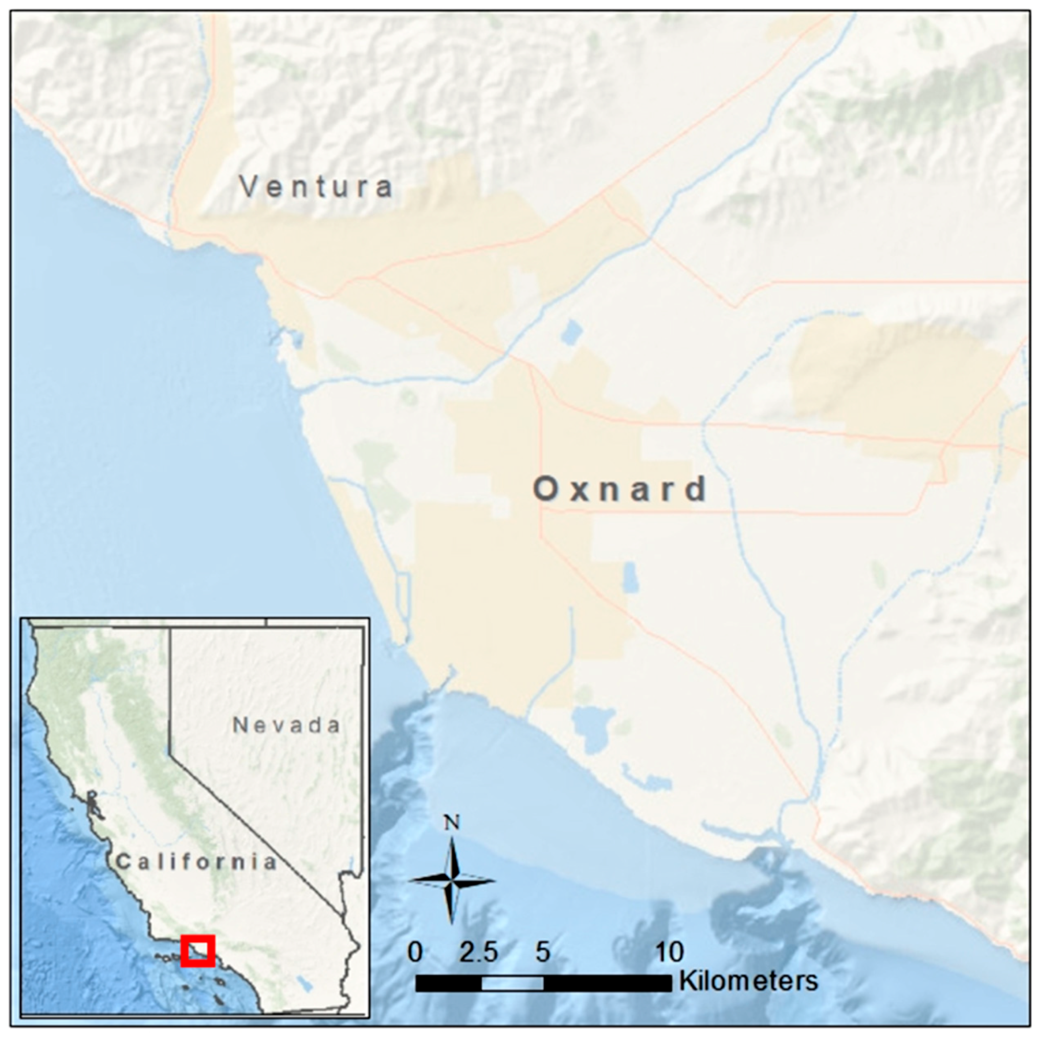
3. Study Location
4. Data
4.1. Radar Imagery
4.2. Bridges
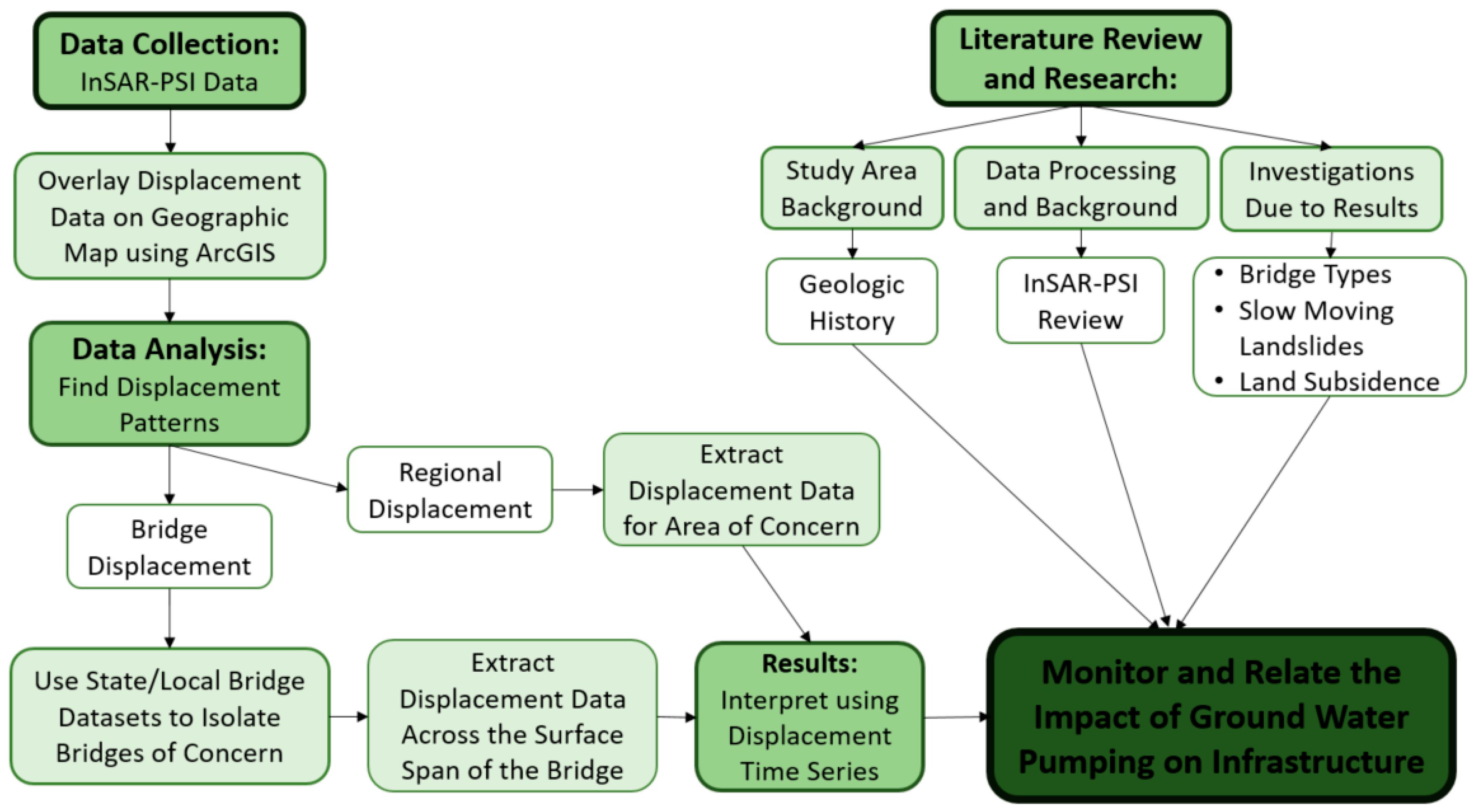
5. Methodology
6. Results and Discussion
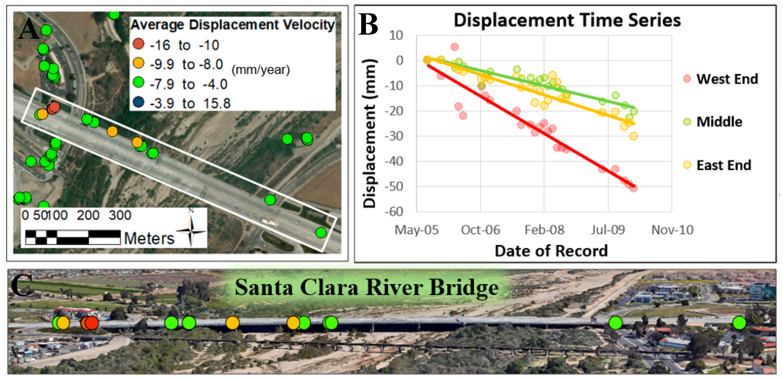
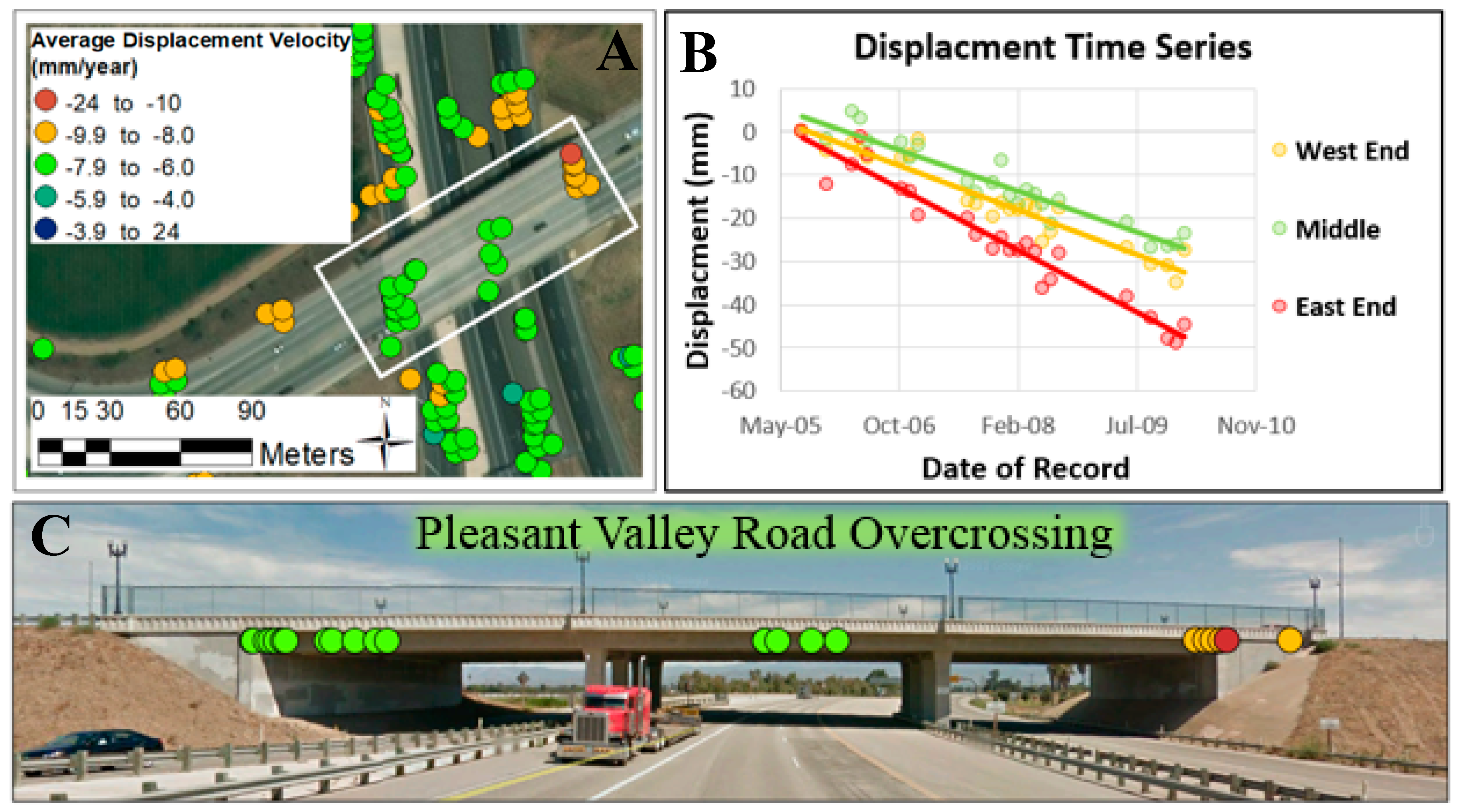
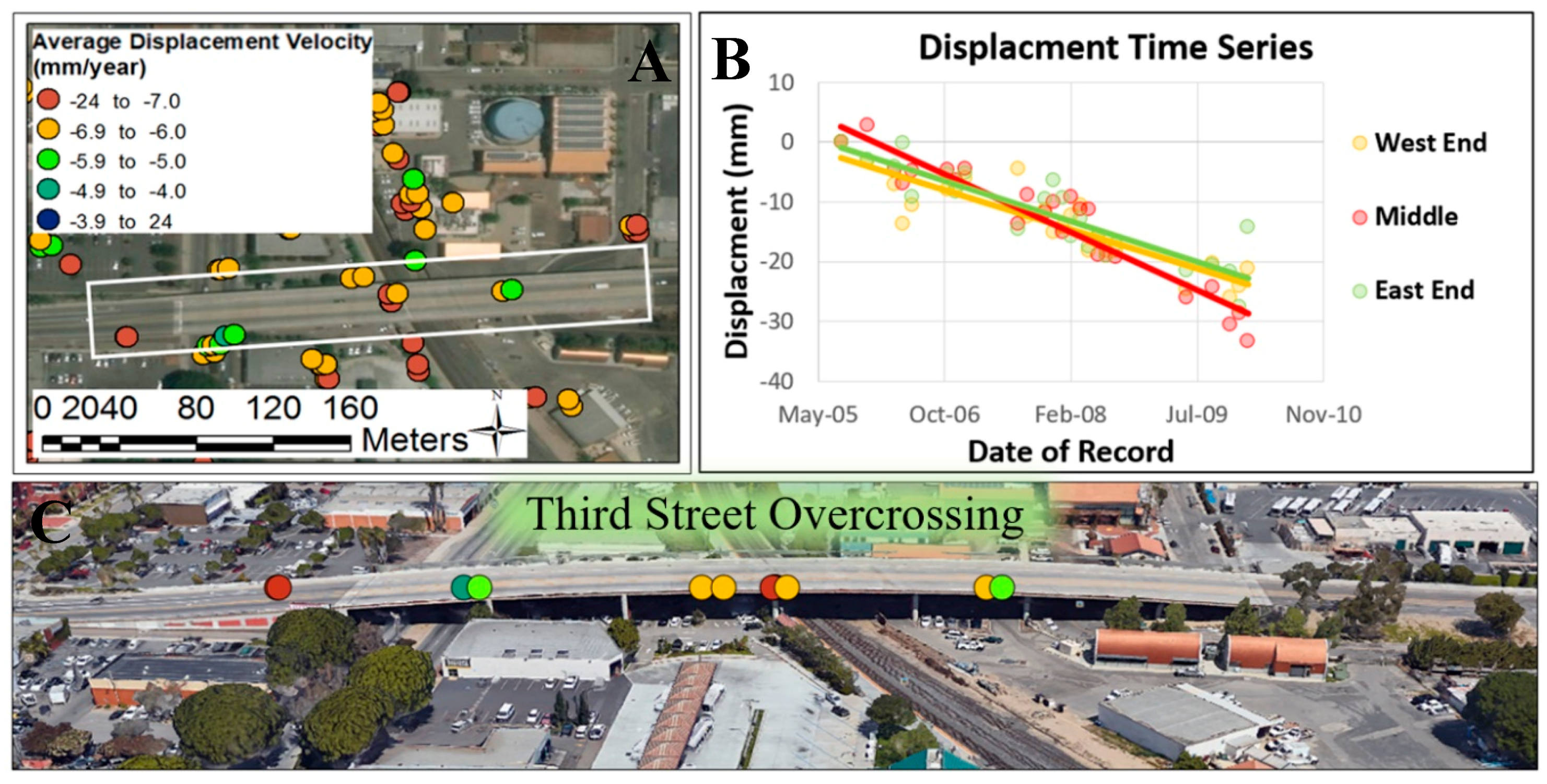
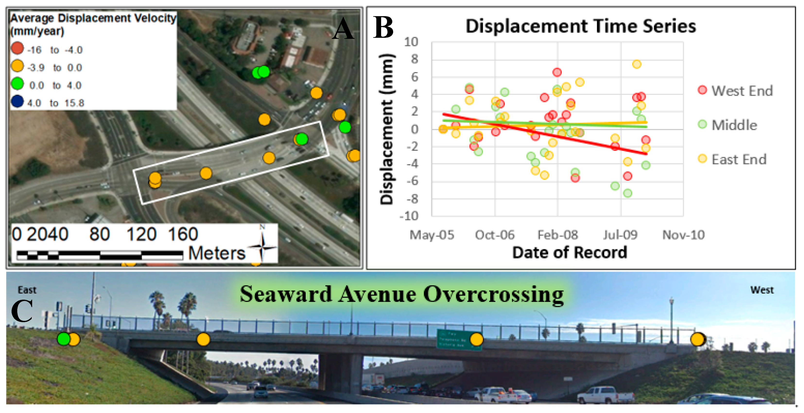
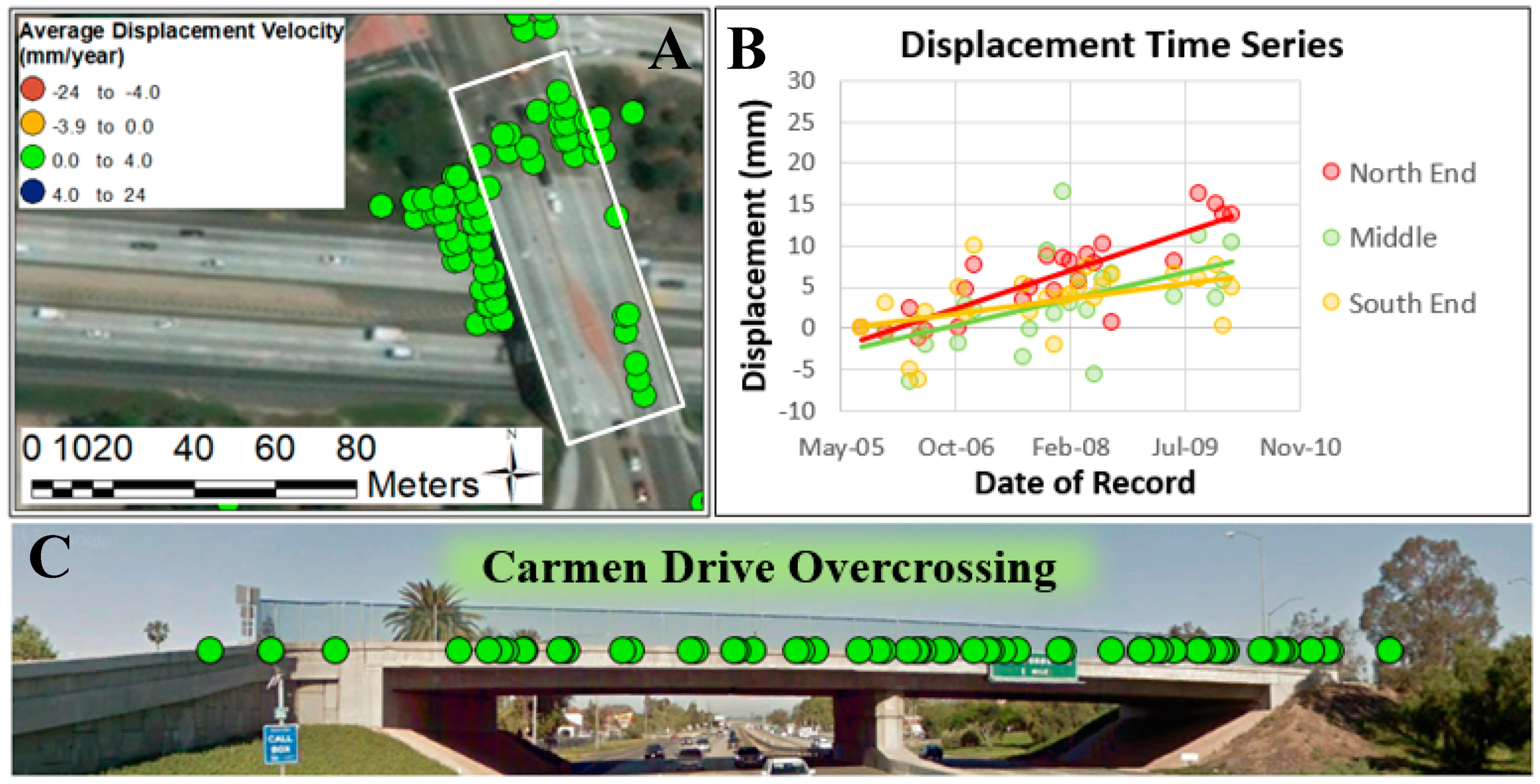
6.1. Bridge Displacement
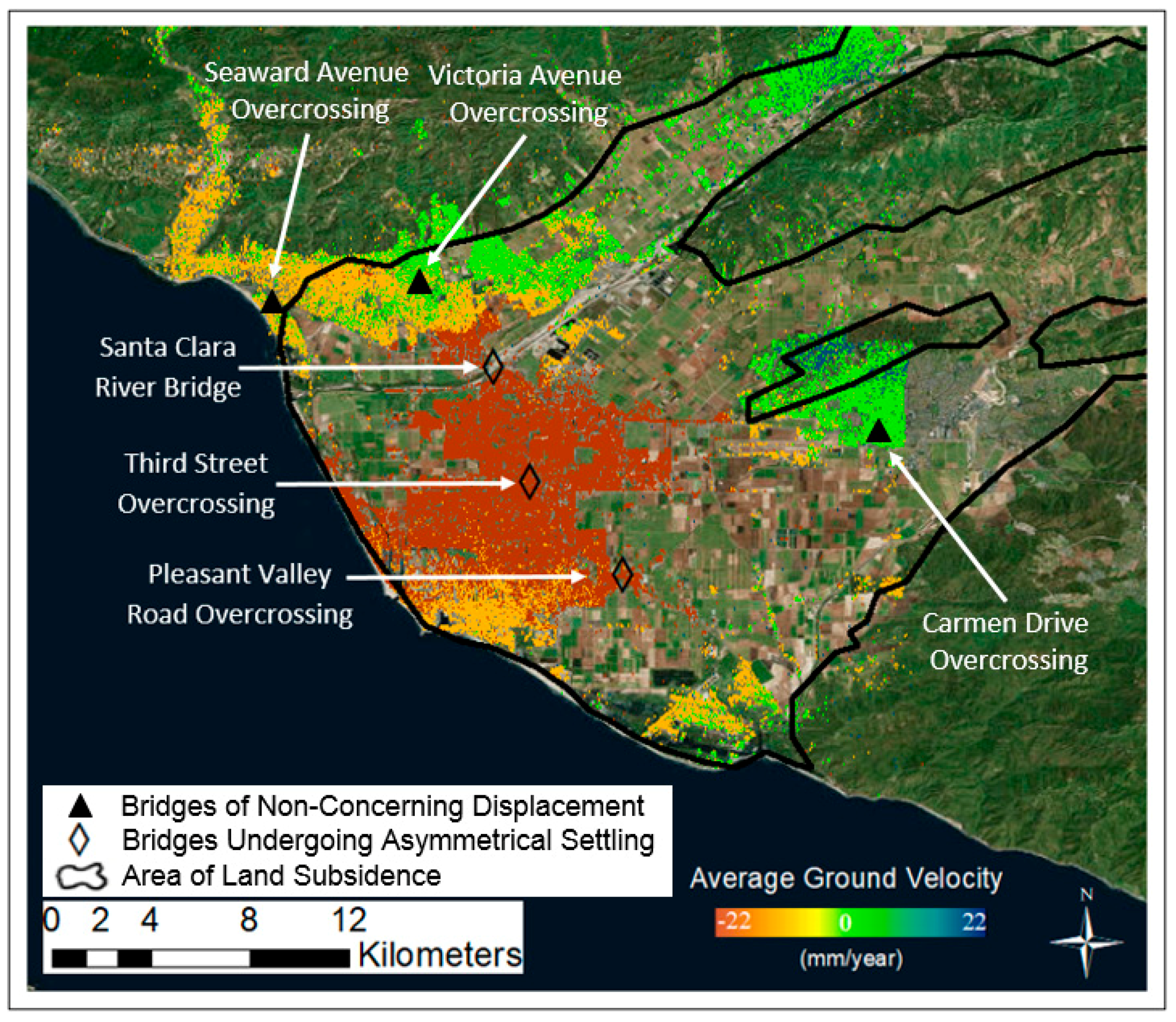
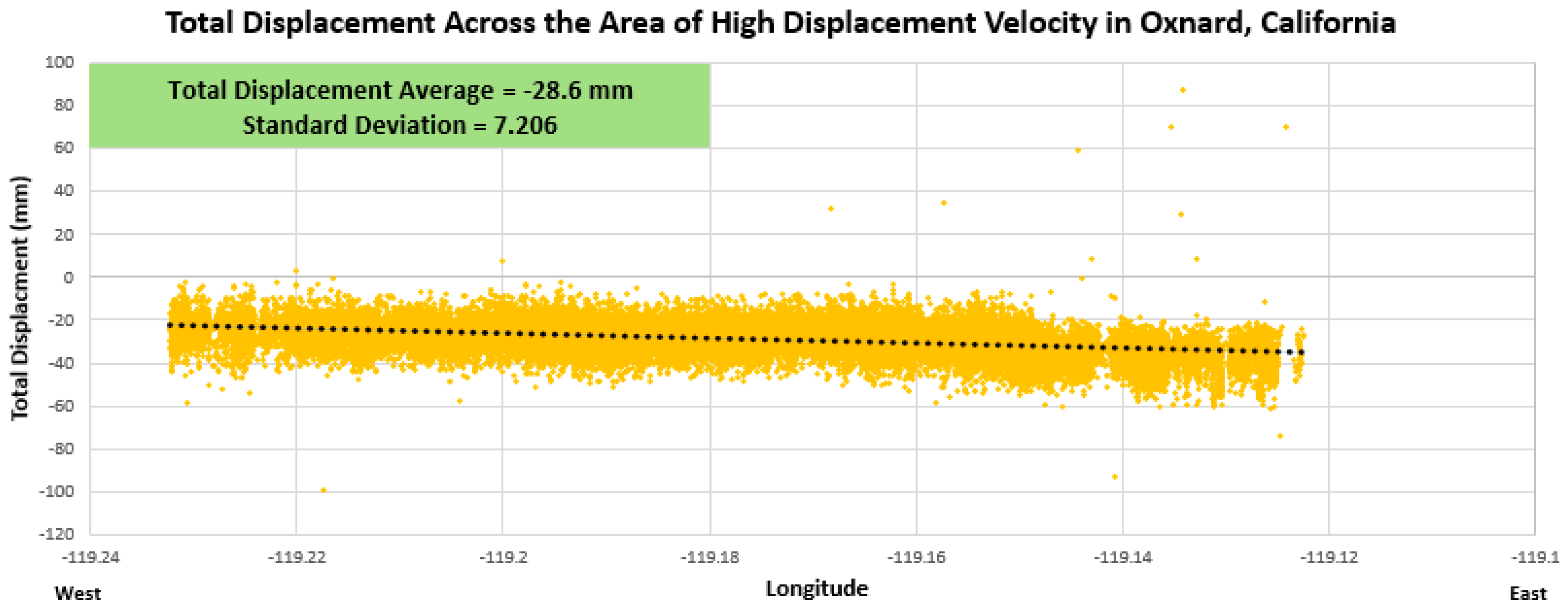
6.2. Regional Ground Displacement & Subsidence
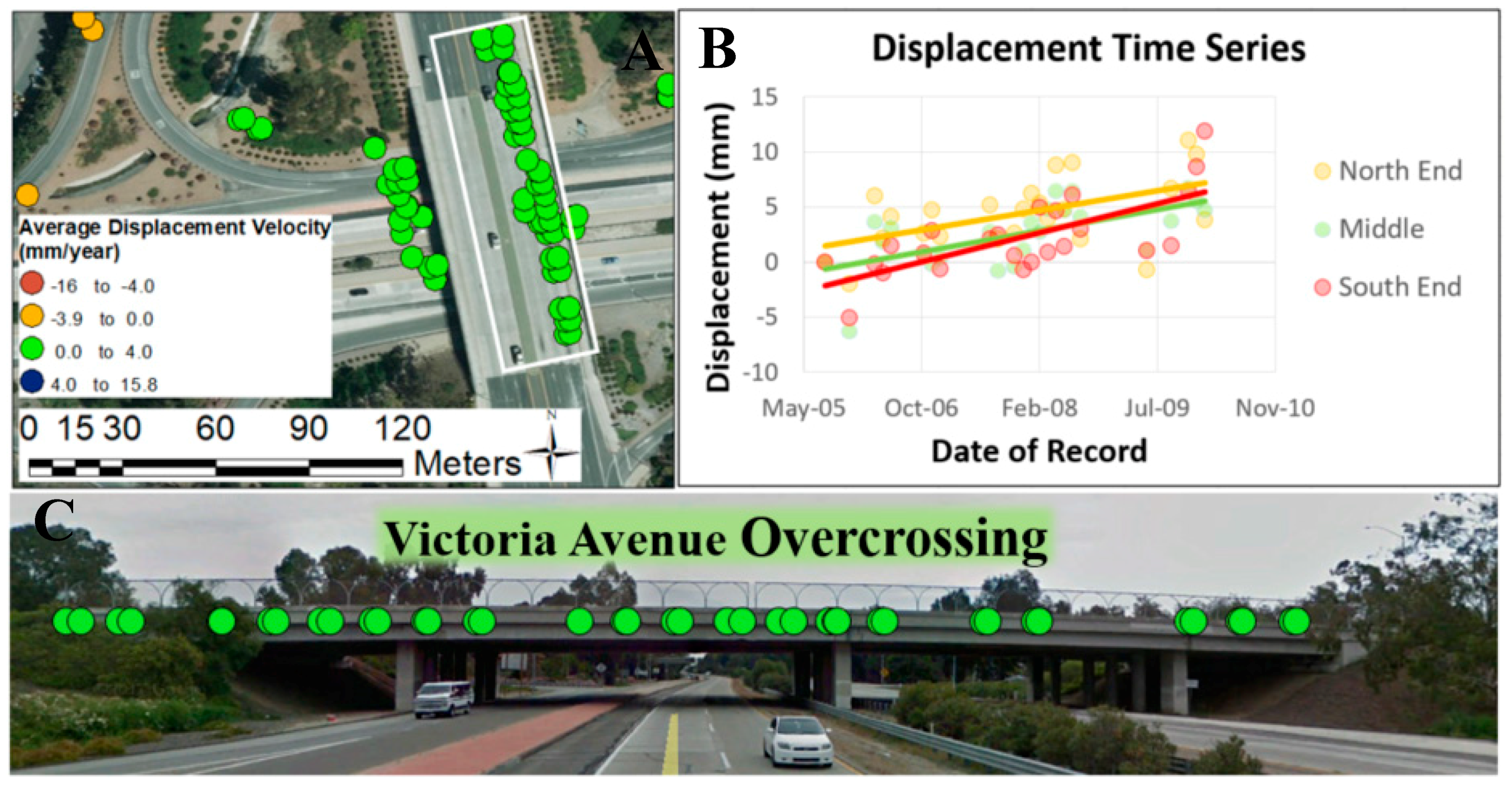
6.3. Stable Bridges
7. Limitations
8. Conclusions
Author Contributions
Funding
Acknowledgments
Conflicts of Interest
References
- Moore, M.; Phares, B.M.; Graybeal, B.; Rolander, D.; Washer, G. Reliability of Visual Inspection for Highway Bridges; No. FHWA-RD-01-020; FHWA: Richmond, VA, USA, 2001; Volume I.
- Sousa, J.J.; Bastos, L. Multi-temporal SAR interferometry reveals acceleration of bridge sinking before collapse. Nat. Hazards Earth Syst. Sci. 2013, 13, 659. [Google Scholar] [CrossRef]
- Zhang, S.; Lippitt, C.D.; Bogus, S.M.; Neville, P.R. Characterizing pavement surface distress conditions with hyper-Spatial resolution natural color aerial photography. Remote Sens. 2016, 8, 392. [Google Scholar] [CrossRef]
- Escobar-Wolf, R.; Oommen, T.; Brooks, C.N.; Dobson, R.J.; Ahlborn, T.M. Unmanned aerial vehicle (UAV)-based assessment of concrete bridge deck delamination using thermal and visible camera sensors: A preliminary analysis. Res. Nondestruct. Eval. 2018, 29, 183–198. [Google Scholar] [CrossRef]
- Bouali, E.H.; Oommen, T.; Vitton, S.; Escobar-Wolf, R.; Brooks, C. Rockfall hazard rating system: Benefits of utilizing remote sensing. Environ. Eng. Geosci. 2017, 23, 165–177. [Google Scholar] [CrossRef]
- Brooks, C.; Dobson, R.J.; Banach, D.M.; Dean, D.; Oommen, T.; Wolf, R.E.; Havens, T.C.; Ahlborn, T.M.; Hart, B. Evaluating the Use of Unmanned Aerial Vehicles for Transportation Purposes (No. RC-1616); TRB: Washington, DC, USA, 2015. [Google Scholar]
- Placzek, G.; Haeni, F.P. Surface-Geophysical Techniques Used to Detect Existing and Infilled Scour Holes Near Bridge Piers: U.S. Geological Survey Water-Resources Investigations Report 95-4009; US Department of the Interior, US Geological Survey: Hartford, CT, USA, 1995; p. 44.
- Zhou, W.; Li, S.; Zhou, Z.; Chang, X. Remote sensing of deformation of a high concrete-faced rockfill dam using InSAR: A study of the Shuibuya dam, China. Remote Sens. 2016, 8, 255. [Google Scholar] [CrossRef]
- Huang, Q.; Monserrat, O.; Crosetto, M.; Crippa, B.; Wang, Y.; Jiang, J.; Ding, Y. Displacement Monitoring and Health Evaluation of Two Bridges Using Sentinel-1 SAR Images. Remote Sens. 2018, 10, 1714. [Google Scholar] [CrossRef]
- Al-Husseinawi, Y.; Li, Z.; Clarke, P.; Edwards, S. Evaluation of the Stability of the Darbandikhan Dam after the 12 November 2017 Mw 7.3 Sarpol-e Zahab (Iran–Iraq Border) Earthquake. Remote Sens. 2018, 10, 1426. [Google Scholar] [CrossRef]
- Zhu, M.; Wan, X.; Fei, B.; Qiao, Z.; Ge, C.; Minati, F.; Vecchioli, F.; Li, J.; Costantini, M. Detection of Building and Infrastructure Instabilities by Automatic Spatiotemporal Analysis of Satellite SAR Interferometry Measurements. Remote Sens. 2018, 10, 1816. [Google Scholar] [CrossRef]
- Zhang, Z.; Wang, C.; Wang, M.; Wang, Z.; Zhang, H. Surface Deformation Monitoring in Zhengzhou City from 2014 to 2016 Using Time-Series InSAR. Remote Sens. 2018, 10, 1731. [Google Scholar] [CrossRef]
- Webb, G.T.; Vardanega, P.J.; Middleton, C.R. Categories of SHM deployments: Technologies and capabilities. J. Bridge Eng. 2014, 20, 04014118. [Google Scholar] [CrossRef]
- López-Higuera, J.M.; Cobo, L.R.; Incera, A.Q.; Cobo, A. Fiber optic sensors in structural health monitoring. J. Lightw. Technol. 2011, 29, 587–608. [Google Scholar] [CrossRef]
- Chen, S.E.; Liu, W.; Dai, K.; Bian, H.; Hauser, E. Remote sensing for bridge monitoring. In Condition, Reliability, and Resilience Assessment of Tunnels and Bridges; Geo-Hunan International Conference Proceedings GSP 214; ASCE: Reston, VA, USA, 2011; pp. 118–125. [Google Scholar]
- Yaghi, S. Integrated Remote Sensing Technologies for Condition Assessment of Concrete Bridges. Ph.D. Thesis, Concordia University, Montreal, QC, Canada, 2014. [Google Scholar]
- Ghodoosi, F.; Bagchi, A.; Zayed, T.; Hosseini, M.R. Method for developing and updating deterioration models for concrete bridge decks using GPR data. Autom. Constr. 2018, 91, 133–141. [Google Scholar] [CrossRef]
- Moselhi, O.; Ahmed, M.; Bhowmick, A. Multisensor Data Fusion for Bridge Condition Assessment. J. Perform. Constr. Facil. 2017, 31, 04017008. [Google Scholar] [CrossRef]
- Bouali, E.H.; Oommen, T.; Escobar-Wolf, R. Mapping of slow landslides on the Palos Verdes Peninsula using the California landslide inventory and persistent scatterer interferometry. Landslides 2018, 15, 439–452. [Google Scholar] [CrossRef]
- Crosetto, M.; Monserrat, O.; Cuevas-González, M.; Devanthéry, N.; Crippa, B. Persistent scatterer interferometry: A review. ISPRS J. Photogramm. Remote Sens. 2016, 115, 78–89. [Google Scholar] [CrossRef]
- Sylvester, A.G.; Smith, R.R. Tectonic transpression and basement-controlled deformation in San Andreas fault zone, Salton Trough, California. AAPG Bull. 1976, 60, 2081–2102. [Google Scholar]
- Sarmap SA. Synthetic Aperture Radar and SARscape: SAR Guidebook; Sarmap SA: Purasca, Switzerland, 2009; pp. 1–274. [Google Scholar]
- Crosetto, M.; Biescas, E.; Duro, J.; Closa, J.; Arnaud, A. Generation of advanced ERS and Envisat interferometric SAR products using the stable point network technique. Photogramm. Eng. Remote Sens. 2008, 74, 443–450. [Google Scholar] [CrossRef]
- Yerkes, R.F.; Campbell, R.H. Preliminary Geologic Map of the Simi 7.5’quadrangle, Southern California, a Digital Database (No. 97-259); US Geological Survey: Reston, VA, USA, 1997.
- Galloway, D.L.; Jones, D.R.; Ingebritsen, S.E. Land Subsidence in the United States (Vol. 1182); US Geological Survey: Reston, VA, USA, 1999.
- California Water Science Center. Areas of Land Subsidence in California. Subsiding Areas in California; 2018. Available online: http://ca.water.usgs.gov/land_subsidence/california-subsidence-areas.html (accessed on 24 January 2018).
- Ferretti, A.; Prati, C.; Rocca, F. Permanent scatterers in SAR interferometry. IEEE Trans. Geosci. Remote Sens. 2001, 39, 8–20. [Google Scholar] [CrossRef] [Green Version]
- Colesanti, C.; Ferretti, A.; Novali, F.; Prati, C.; Rocca, F. SAR monitoring of progressive and seasonal ground deformation using the permanent scatterers technique. IEEE Trans. Geosci. Remote Sens. 2003, 41, 1685–1701. [Google Scholar] [CrossRef]
- Colesanti, C.; Ferretti, A.; Prati, C.; Rocca, F. Monitoring landslides and tectonic motions with the Permanent Scatterers Technique. Eng. Geol. 2003, 68, 3–14. [Google Scholar] [CrossRef]
- Bouali, E.H.; Oommen, T.; Escobar-Wolf, R. Structure mapping through spatial and temporal deformation monitoring using persistent scatterer interferometry and geographic information systems. Geotech. Front. 2017, 2017, 509–519. [Google Scholar]
- Bru, G.; Herrera, G.; Tomás, R.; Duro, J.; De la Vega, R.; Mulas, J. Control of deformation of buildings affected by subsidence using persistent scatterer interferometry. Struct. Infrastruct. Eng. 2013, 9, 188–200. [Google Scholar] [CrossRef]
- Bianchini, S.; Pratesi, F.; Nolesini, T.; Casagli, N. Building deformation assessment by means of persistent scatterer interferometry analysis on a landslide-affected area: The Volterra (Italy) case study. Remote Sens. 2015, 7, 4678–4701. [Google Scholar] [CrossRef]
- Ferretti, A.; Tamburini, A.; Novali, F.; Fumagalli, A.; Falorni, G.; Rucci, A. Impact of high resolution radar imagery on reservoir monitoring. Energy Procedia 2011, 4, 3465–3471. [Google Scholar] [CrossRef]
- Di Martire, D.; Iglesias, R.; Monells, D.; Centolanza, G.; Sica, S.; Ramondini, M.; Pagano, L.; Mallorquí, J.J.; Calcaterra, D. Comparison between different SAR interferometry and ground measurements data in the displacement monitoring of the earth-dam of Conza della Campania (Italy). Remote Sens. Environ. 2014, 148, 58–69. [Google Scholar] [CrossRef]
- Vasco, D.W.; Ferretti, A.; Novalli, F. Reservoir monitoring and characterization using satellite geodetic data: Interferometric synthetic aperture radar observations from the Krechba field, Algeria. Geophysics 2008, 73, WA113–WA122. [Google Scholar] [CrossRef]
- Sousa, J.J.; Ruiz, A.M.; Bakoň, M.; Lazecky, M.; Hlaváčová, I.; Patrício, G.; Delgado, J.M.; Perissin, D. Potential of C-Band SAR Interferometry for Dam Monitoring. Proc. Comput. Sci. 2016, 100, 1103–1114. [Google Scholar]
- Liu, G.; Jia, H.; Zhang, R.; Zhang, H.; Jia, H.; Yu, B.; Sang, M. Exploration of subsidence estimation by persistent scatterer InSAR on time series of high resolution TerraSAR-X images. IEEE J. Sel. Top. Appl. Earth Obs. Remote Sens. 2011, 4, 159–170. [Google Scholar] [CrossRef]
- Huang, Q.; Crosetto, M.; Monserrat, O.; Crippa, B. Displacement monitoring and modelling of a high-speed railway bridge using C-band Sentinel-1 data. ISPRS J. Photogramm. Remote Sens. 2017, 128, 204–211. [Google Scholar] [CrossRef]
- Lazecky, M.; Perissin, D.; Bakon, M.; de Sousa, J.M.; Hlavacova, I.; Real, N. Potential of satellite InSAR techniques for monitoring of bridge deformations. In Proceedings of the 2015 Joint Urban Remote Sensing Event (JURSE), Lausanne, Switzerland, 30 March–1 April 2015; pp. 1–4. [Google Scholar]
- Soergel, U.; Cadario, E.; Gross, H.; Thiele, A.; Thoennessen, U. Bridge detection in multi-aspect high-resolution interferometric SAR data. In Proceedings of the 6th European Conference on Synthetic Aperture Radar, Dresden, Germany, 16–18 May 2006. [Google Scholar]
- Wegner, J.D.; Soergel, U. Bridge height estimation from combined high-resolution optical and SAR imagery. Int. Arch. Photogramm. Remote Sens. Spat. Inf. Sci. 2008, 379, 1071–1076. [Google Scholar]
- Tofani, V.; Raspini, F.; Catani, F.; Casagli, N. Persistent Scatterer Interferometry (PSI) technique for landslide characterization and monitoring. Remote Sens. 2013, 5, 1045–1065. [Google Scholar] [CrossRef]
- Cigna, F.; Bianchini, S.; Casagli, N. How to assess landslide activity and intensity with Persistent Scatterer Interferometry (PSI): The PSI-based matrix approach. Landslides 2013, 10, 267–283. [Google Scholar] [CrossRef]
- Parcharidis, I.; Foumelis, M.; Kourkouli, P.; Wegmuller, U.; Lagios, E.; Sakkas, V. Continuous Risk Assessment of Structures in Areas of Ground Deformation Susceptibility by Persistent Scatterers InSAR: Preliminary Result of the Rio-Antirio Bridge (Greece). In Proceedings of the ESA Fringe 2007 Worshop, Frascati, Italy, 26–30 November 2007. [Google Scholar]
- Sousa, J.J.; Hlaváčová, I.; Bakoň, M.; Lazecký, M.; Patrício, G.; Guimarães, P.; Ruiz, A.M.; Bastos, L.; Sousa, A.; Bento, R. Potential of multi-temporal InSAR techniques for bridges and dams monitoring. Procedia Technol. 2014, 16, 834–841. [Google Scholar] [CrossRef]
- Owen, G.; Moretti, M.; Alfaro, P. Recognising triggers for soft-sediment deformation: Current understanding and future directions. Sediment. Geol. 2011, 235, 133–140. [Google Scholar] [CrossRef]
- California Log of Bridges on State Highways. California Department of Transportation. Available online: www.dot.ca.gov/hq/structur/strmaint/brlog2.htm (accessed on 6 February 2018).
- Google Earth. Bridge Photo Source; Google: Mountain View, CA, USA, 2017. [Google Scholar]


| Location on Bridge | Displacement due to Regional Patterns (mm) | Site-Based/Structural Movement (mm) | Total Displacement (mm) (Downward Direction) |
|---|---|---|---|
| East End | ~20–30 | ~5 | 25–35 |
| Middle | 20 | 0 | 20 |
| West End | ~20–30 | ~20 | 50 |
© 2018 by the authors. Licensee MDPI, Basel, Switzerland. This article is an open access article distributed under the terms and conditions of the Creative Commons Attribution (CC BY) license (http://creativecommons.org/licenses/by/4.0/).
Share and Cite
DePrekel, K.; Bouali, E.H.; Oommen, T. Monitoring the Impact of Groundwater Pumping on Infrastructure Using Geographic Information System (GIS) and Persistent Scatterer Interferometry (PSI). Infrastructures 2018, 3, 57. https://0-doi-org.brum.beds.ac.uk/10.3390/infrastructures3040057
DePrekel K, Bouali EH, Oommen T. Monitoring the Impact of Groundwater Pumping on Infrastructure Using Geographic Information System (GIS) and Persistent Scatterer Interferometry (PSI). Infrastructures. 2018; 3(4):57. https://0-doi-org.brum.beds.ac.uk/10.3390/infrastructures3040057
Chicago/Turabian StyleDePrekel, Kirsten, El Hachemi Bouali, and Thomas Oommen. 2018. "Monitoring the Impact of Groundwater Pumping on Infrastructure Using Geographic Information System (GIS) and Persistent Scatterer Interferometry (PSI)" Infrastructures 3, no. 4: 57. https://0-doi-org.brum.beds.ac.uk/10.3390/infrastructures3040057