Force Performance Analysis of Pile Behavior of the Lateral Load
by
 , and
, and
Touré Youssouf
1,*, 
Tianlai Yu
1,
Dembélé Abdramane
2,
Assogba Ogoubi Cyriaque
3 and
and
Diakité Youssouf
4 1
College of Civil Engineering, Department of Civil Engineering, Northeast Forestry University, No.26 Hexing Road, Xiangfang District, Harbin 150040, China
2
Department of Automation Harbin Engineering University Heilongjiang Province, Harbin 150001, China
3
School of transportation science and engineering, Harbin Institute of technology, Harbin 150090, China
4
School of Civil engineering, Harbin Institute of Technology, Harbin 150090, China
*
Author to whom correspondence should be addressed.
Infrastructures 2019, 4(2), 13; https://0-doi-org.brum.beds.ac.uk/10.3390/infrastructures4020013
Submission received: 27 January 2019
/
Revised: 20 March 2019
/
Accepted: 25 March 2019
/
Published: 28 March 2019
Abstract
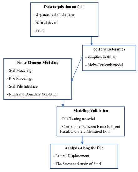
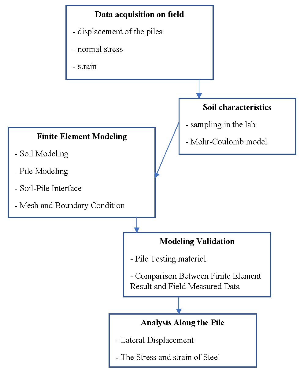
:This study was focused on the performance of the pile force at the lateral load of an arched bridge. The effect of the compression of arch bridges creates a large horizontal load. Therefore, it is one of the most important factors in the dimensioning of piles. The study aims to make a comparative study between the results obtained in the field, and those obtained by a 3D model defined as a Finite Element (FE) of a drilled pile, subjected to different lateral loads applied at exact time intervals. Moreover, the study was intended to determine the influence of the lateral load applied to a different pile diameter using the FE model. Thus, the unified FEA software Abaqus™ by Dassault systèmes® carried out various processing procedures, namely soil FE modeling, pile FE modeling, soil-pile interface, Mesh, and boundary conditions, to carry out an effective and predictive piles behavior analysis. Based on the Mohr-Coulomb criterion, the soil is considered to be stratified with elastoplastic behavior, whereas the Reinforcement Concrete Pile (RCP) was assumed to be linear isotropic elastic, integrating the concrete damage plasticity. Since the bridge is an arched bridge, the lateral load induced was applied to the head of the piles through a concentrated force to check the pile strength, for which the displacement, stress and strain were taken into account throughout, along the pile depth. The lateral displacement of the pile shows a deformation of the soil as a function of its depth, with different layers crossed with different lateral loads applied. Thus, from the study comparing the results of the FE measurements with the data measured in the field, added to the statistical analyses are as follows: Decrease of the displacement and stress according to the diameter, taking into account the different diameter. The foundations receive loads of the superstructure to be transmitted to the ground. Thus, the piles are generally used as a carrier transmitting loads on the ground. One of the important factors in the durability of the bridge depends more on the strength of these piles. This makes it necessary to study the reinforced concrete foundations because of their ability to resist loads of the structure, and the vertical and lateral loads applied to the structure. This implies an evaluation of the responses of the RCP according to the different lateral loads.
1. Introduction
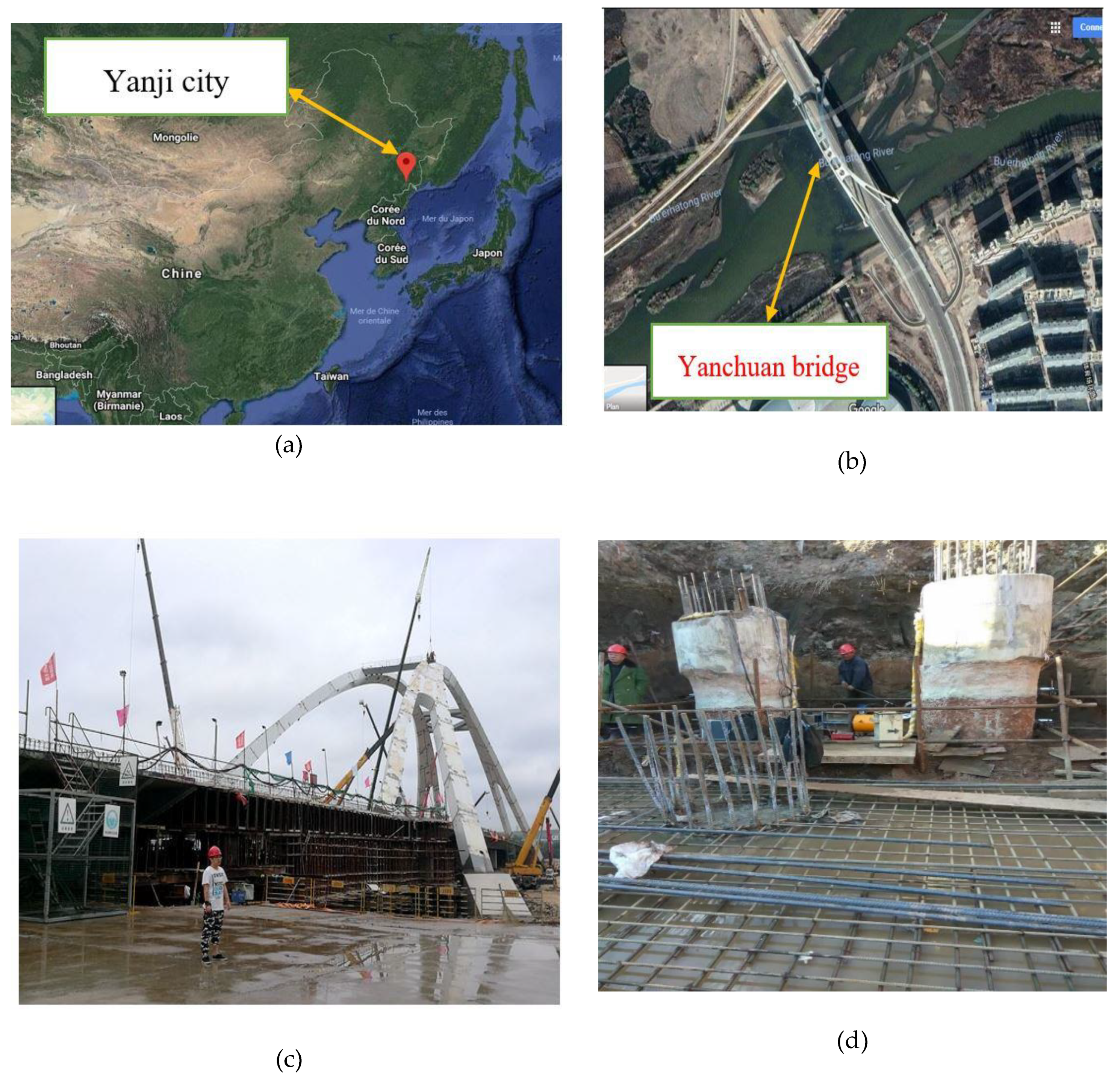
The lateral load on the pile was performed on the Yanchuan Bridge in Jilin province Yanji city, across the Burghardtong River, China. It extends over a complete length of 324. 86 m across the South Burghardtong River (Figure 1) in Figure 1 a,b,c and d it can show the location of city, construction, view of bridge and test pile. The design of the arch was chosen from an architectural purpose of view, so that the bridge can be integrated into the natural site to extend the characteristics of the landscape of the bridge, and decongest the speedily developing areas around the river, to assist increased traffic in the central city. The site is located around the river at the placement of the bridge as shown in Figure 1. Therefore, it will not be only a significant part of the infrastructure for this event, but it will also have to act as an exhibit area for Chinese engineering. The planning of foundations on simple supports is classical (drilled piles). However, the design of arch foundations is quite complex, due to the low stiffness and solidity of the soil characteristics; therefore, this study is based on force performance analysis of pile behavior of the lateral load. For the arch bridge, the lateral load test is unavoidable because of the yearly temperature changes comprised between 30 °C to −30 °C.
Reinforced concrete piles or drilled shafts are a kind of bridge substructure within which piles or columns are continuously extended below the extent of the superstructure. This, alongside with the depth of the soil modulus and the limiting values of pile-soil contact pressure, needs to be prespecified. For the numerical methods, the analysis is done by using finite elements or finite variations. These methods will presently tackle the complete three-dimensional (3D) drawback, considering the precise geometry, soil-structure interaction and pile effects, though such ways are in theory the most rigorous [1,2,3].
Reinforced concrete could be a standard material created by combining cement and forms with the aim of compensating for the relatively low durability and stability of Reinforcement Concrete Pile (RCP). Reinforcements that are mostly steel bars represent all the interconnected bars in the concrete that reinforce concrete development. Both materials have a complete consolidation because there is almost no slippage between the two, such that the concrete acts in a way as a protective layer for the steel bar against corrosion.
Despite the high cost of reinforcing steel, it remains the recommended one for construction. It is, therefore, necessary to review the likelihood of reducing this material to a minimum throughout pile construction. In the past, piles were unquestionably strengthened [4]. Nowadays, the designers are minimizing the length of reinforcing bars; therefore, they are scaling back the number of piles [5,6,7,8,9,10,11,12,13,14,15,16,17,18,19,20]. This reduction needs excellent separation for the cases wherever the piles would entirely or partly require reinforcement, and in cases where the reinforcement has been eliminated. From the creation survey on the codes and their field findings recommendations, codes are required to provide specifications and limitations for the proportion of bars that ought to be provided within the pile cross-sectional area [8,10,21,22,23,24,25]. However, the depth of extension of this reinforcement on the pile is not sufficient, and is left to the designer’s discretion. The main objectives of this study are: (i) On one side, develop a 3D element model that integrates the viscous plastic behavior of the stratified soil (not homogeneous), and on the other hand, the elastoplastic behavior with concrete damage plasticity. This should be done in order to accurately simulate the instrumented RCP system used at Yanchuan Bridge which was designed to last for over 100 years, according to current Chinese building foundation pile testing technical specifications (JGJ106-2003); (ii) to determine parameters such as lateral displacement, stress and strain along the pile while subjected to diverse lateral loading; (iii) finally, to investigate the effect of an influential parameter such as the diameter of the RCP on its mechanical response.
2. Basic Theory of Reinforcement Concrete Pile on a Lateral Load
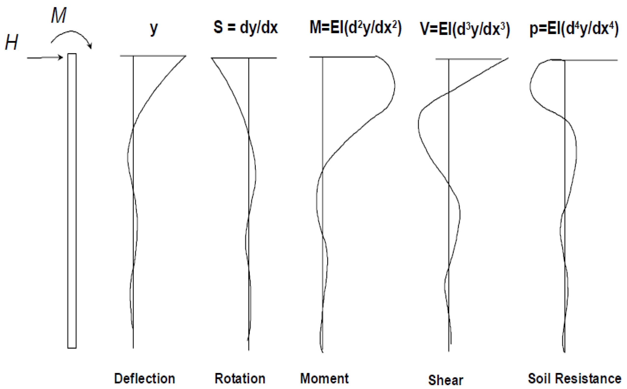
Several researchers have developed the speculation on (p–y) curves for sand to explain the connection between soil resistance and the lateral displacement of the pile below lateral load [26,27]. In this curve, the (p) denotes the soil reaction and (y) is a deflection of the pile. The bending of the pile is described in equation 6 for beam bending, ad it can be seen in Figure 2.
Where,
- y = deflection of the pile
- S = slope of the deflected pile
- M = moment of the pile
- V = Shear
- P = Soil reaction
- Ep = elasticity modulus
- Ip = moment of inertia of the pile
- QA = load
- z = depth below the pile top
The (p–y) curves are realized using the Winkler approach with uncoupled springs along the pile, where each is supporting a pile distribution. For each spring, a non-linear (p–y) curve is made. The curves were adopted and utilized in current strategies for designing lateral loaded piles within the standard codes [26,28]. These methods are incredibly empirical, and in each area unit they are fitted by solely a few all-out experiments represented by Salman et al [8,9,26,29,30]. The procedure for making the (p–y) curves for the cyclic lateral load on monopiles in the sand is shown by Rasmussen et al [26].
One of the main approaches for calculating the ultimate displacement because of soil yielding is the beam-on-foundation approach, where the soil is treated as plastic, and its lateral capacity is often determined from its resistance [6,9,15]. This method does not predict pile response, since the soil resistance of the analysis is developed by empirical observation, and is fitted to the numerical analysis results to satisfy the results. Another disadvantage of the (p–y) curve is that a curve developed for a particular site is not appropriate for one more site. In different countries, every site that constructs its (p–y) curve is relying on the properties of the soil as a load, pile checks to predict lateral pile response accurately. This technique is therefore costly because each site requires testing the pile load [9]. An Associate in soil resolution supported an energy-based technique leading to a collection of governing equations and boundary conditions. The collection of governing equations and boundary conditions, which represent the deformation of the pile and soil below static lateral load, has been utilized by Hashem et al [9,31,32,33,34] in homogeneous soil linear elastic, and Hashem et al [9,35] in multi-layered nonlinear and linear elastic soil. These equations were resolved numerically employing a finite distinction technique, whereas [9], used an equivalent technique to predict the deformation of a pile within inhomogeneous linear elastic soil below dynamic lateral loads. To predict pile displacement because of lateral load, three approaches are often used: The cantilever technique, Winkler’s technique, and the elastic continuum technique. The cantilever method was developed by Hashem [9]. In this methodology, the soil reaction is neglected, and the easy cantilever theory is employed to calculate the deformation. The distinction in the behavior of flexible and rigid piles has much essential influence on soil behavior and the development of a “toe-kick” is essential for rigid piles.
3. Finite Element Modeling (FEM)
This section presents the three-dimensional model established through a finite element program the unified FEA software Abaqus™ by Dassault systèmes® to investigate the behavior of a reinforced concrete pile subject to lateral load. A Concentrated load force was applied on the pile head to represent the field loading condition (Jack Force) better. The symmetric geometry of the pile and the lateral deflection of the pile head was assessed under lateral loading, when such a load was applied on the pile head. According to the solid mechanics formulations, the amount of lateral deflection can be found from Beam Flexure Theory. The pile placed in the soil continued up to the bedrock or hard layer. Therefore, it is often thought of as a cantilever beam [34,36,37,38,39].
3.1. Soil Finite Element Modeling
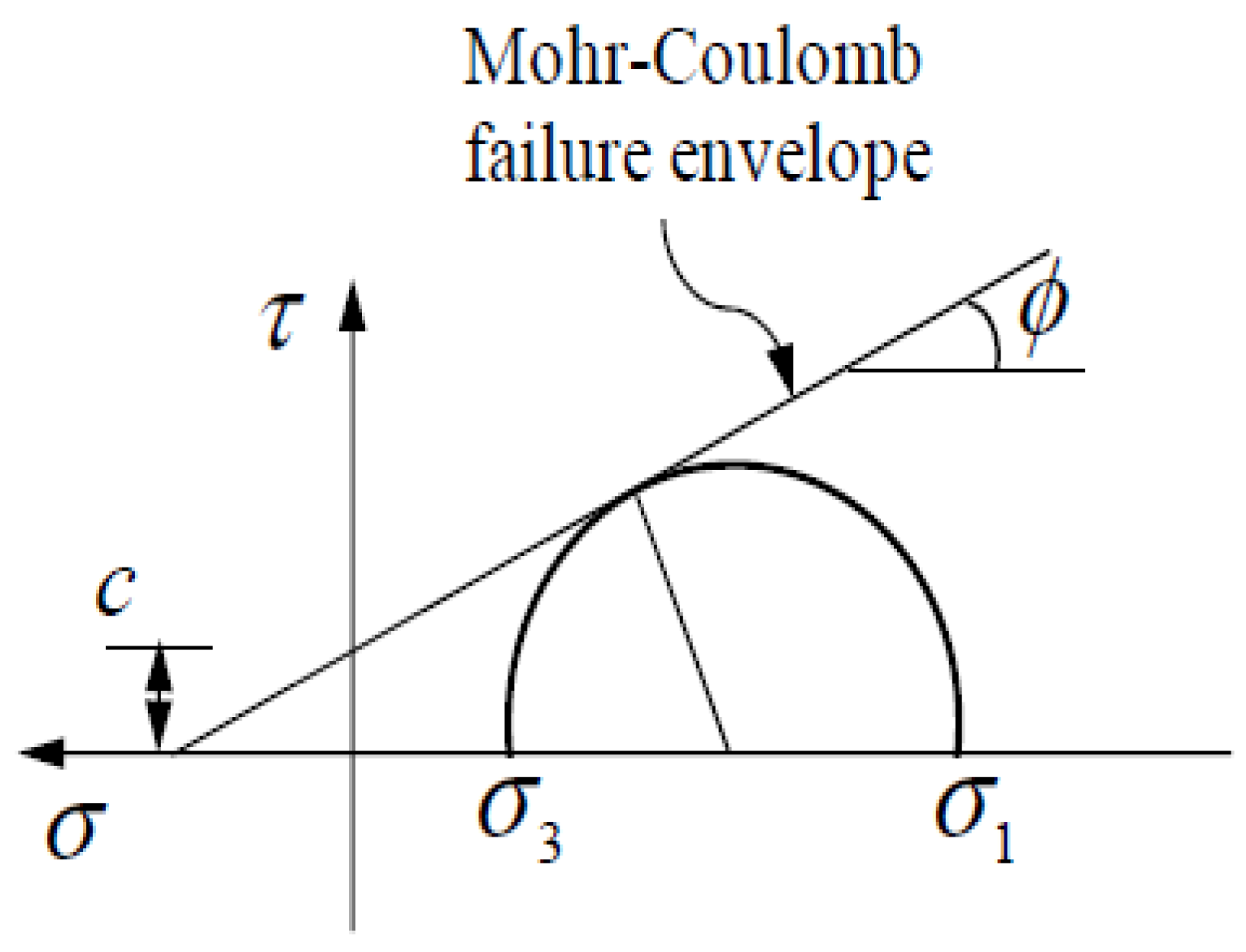
The upper, secondary, tertiary and quaternary formations of the soil consist of layers of resistant heavy weathered sandstone with different thicknesses as follows: Top, 6.5 m, second, 3.1 m, tertiary, 3.2 m, and quaternary, 0.8 m. The fifth layer is intense to very dense metamorphic siltstone mudstone (8.4 m). The physical and mechanical properties of the soil are indicated in Table 1. These values are given by the geotechnical investigation report of the field provided by the Institute of Geological Investigation of the Province of Jilin in China. It is important to emphasize that the soil stratification adopted is comparable to that of the soil in Jilin Province (North-East China) where the “Yan Song Bridge” was constructed. With the development of advanced computation tools, the finite element method is widely used to describe the behavior of complex geo-materials. Most complexes in a different loading handled the difficulties in the digital application and the identification parameters of the element using the standard materials test procedure [21]. Elastoplastic constitutive model with models Mohr-Coulomb failure criterion are often used to integrate the mechanical behavior of the soil in finite element analysis. By reason of its simplicity and its complete accuracy in case of rupture, which is dependent on the maximum principal stress σ1 and the minimum principal stress σ3 as shown in Figure 3. The Mohr-Coulomb model is described by the cohesion c and internal friction angle ∅ [31,40].
When the distribution in the space of three-dimensional stress, the case of rupture is formed in an irregular hexagonal pyramid.
The Mohr-Coulomb model is widely used in geotechnical engineering practice. In this simulation, the Mohr-Coulomb model has been adopted to represent the structural and functional behavior of the soil. In Abaqus 2017, three parameters are required to define the behavior of the soil. These parameters are the Density γ ‘, friction angle Φ and Cohesion C. The elastic-modulus was taken according to the different soil properties with depth. The soil was divided into five layers with constant properties for every layer, as depicted in Table 1.
3.2. Single Pile Finite Element Modeling
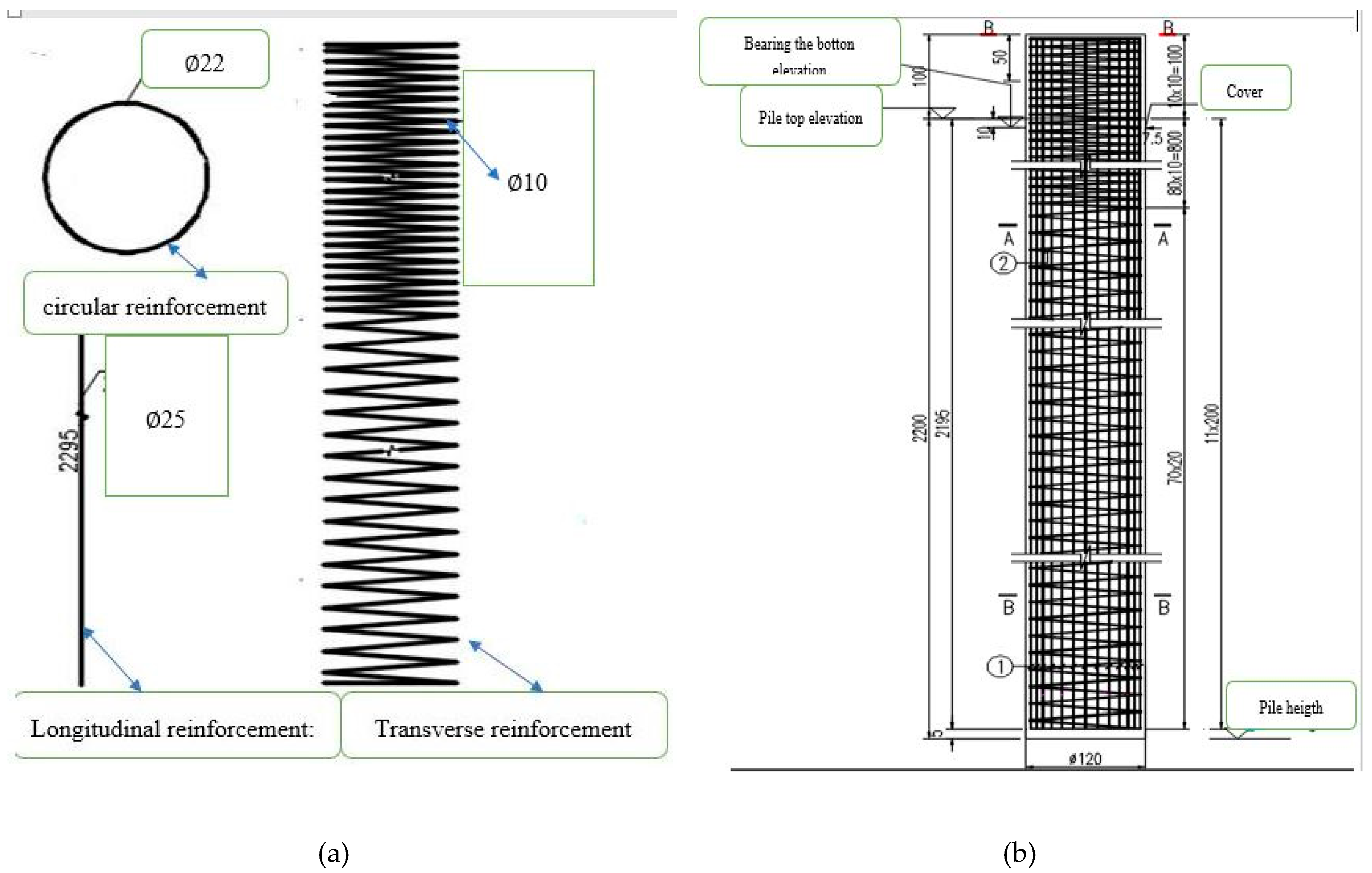
In this numerical study, the pile is modeled as a 3D structural element consisting of a reinforced concrete material; therefore, the characteristics of the pile are depicted in the following, Table 2 and Table 3. It can be noted that the reinforced concrete pile, and the choice of characteristics as follows, and according to the execution plans, are: The longitudinal, circular and transverse reinforcement are high-adhesion steel (HA). The reinforcements chosen for the FE model are in accordance with the reinforcement used on the field, and are as follows: Longitudinal reinforcement: HA 25; circular reinforcement HA 20; Transverse armatures HA 10, which is shown in Figure 4a. Once a bent deck pile is subjected to a lateral load, plastic hinges might form at the top of the pile and below the ground. Once the pile is used to form pile bridge dents, each of those possible hinge positions can have completely different properties and behavior. In the case of the upper hinges and the area between the steel tubes, the tube only provides containment and shear strength, whereas the longitudinal bars mainly provide flexural strength. Conversely, for in-grounds hinges, the steel tube will provide not only shear resistance and containment of the concrete, but also bending resistance. As a result, the moment capacity and stiffness of the belowground hinges in a pile will be considerably larger than those expected in the upper hinges.
The reinforcement is FE 400 steel, and was supplied by the Changchun manufacturing company in Jilin province, China, and the concrete has a compressive strength of 30 MPa.
3.3. Soil-Pile Interface
The surface contact of the pile-soil tangentially embraces the load transfer mechanisms in each direction. The applied lateral load force is transferred correctly to the ground when the pile and the surrounding soil surface are tightly in contact. Otherwise, it becomes insignificant (close to zero). This type of traditional contact behavior will be present by (hard) contact choice provided by Abaqus™.
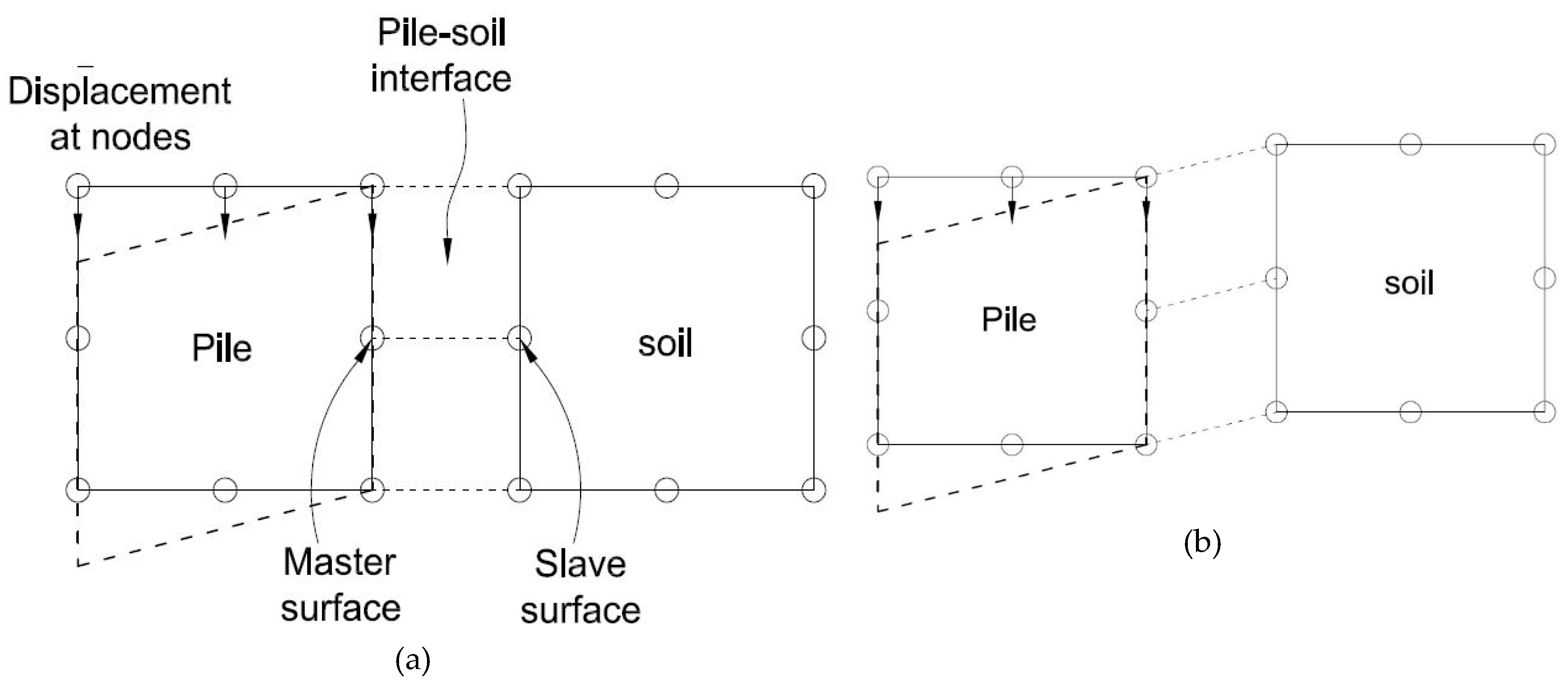
The tangent behavior will vary from rough contact with no relative slippage between soil flank and pile, to slippery resistance conditions with no friction development on the shaft of the pile. For contact between these two typical cases, the pile resistance model in Abaqus™ will be chosen to depict the interaction at the pile-soil interface with a prescribed resistance constant µ. These two ideal contact conditions may also be completed through the following cases: With resistance, and without resistance. The soil-pile interface modeling is extremely essential due to its influence on the pile response below lateral loading within the soil-pile interaction, where the surrounding soil and the pile elements are assumed deformable [30,34,37,40,41,42,43,44,45]. The surface of pile elements and soil elements have a contact that the surface of pile components is selected as “Master surface,” and therefore the surfaces of soil elements are defined as “Slave surface.” In Abaqus™, these surfaces are known as the contact pair, and they are depicted in Figure 5. In order to take account, the quality and the type of soil, following the suggestions of API (1991) and Gireesha (2011), and after several sensitive analyses, the coefficient of friction between concrete and sand relating shear stress to the normal stress was assumed to be 0.75 throughout the analysis [34]. The “penalty function method” was utilized to represent the contact with normal contact stiffness (Kn). Once the tangent shear stress in pile-soil interface surpasses the shear resistance, relative slip between pile and soil happens. The interaction parameters used are shown in Table 4.
3.4. Mesh and Boundary Condition
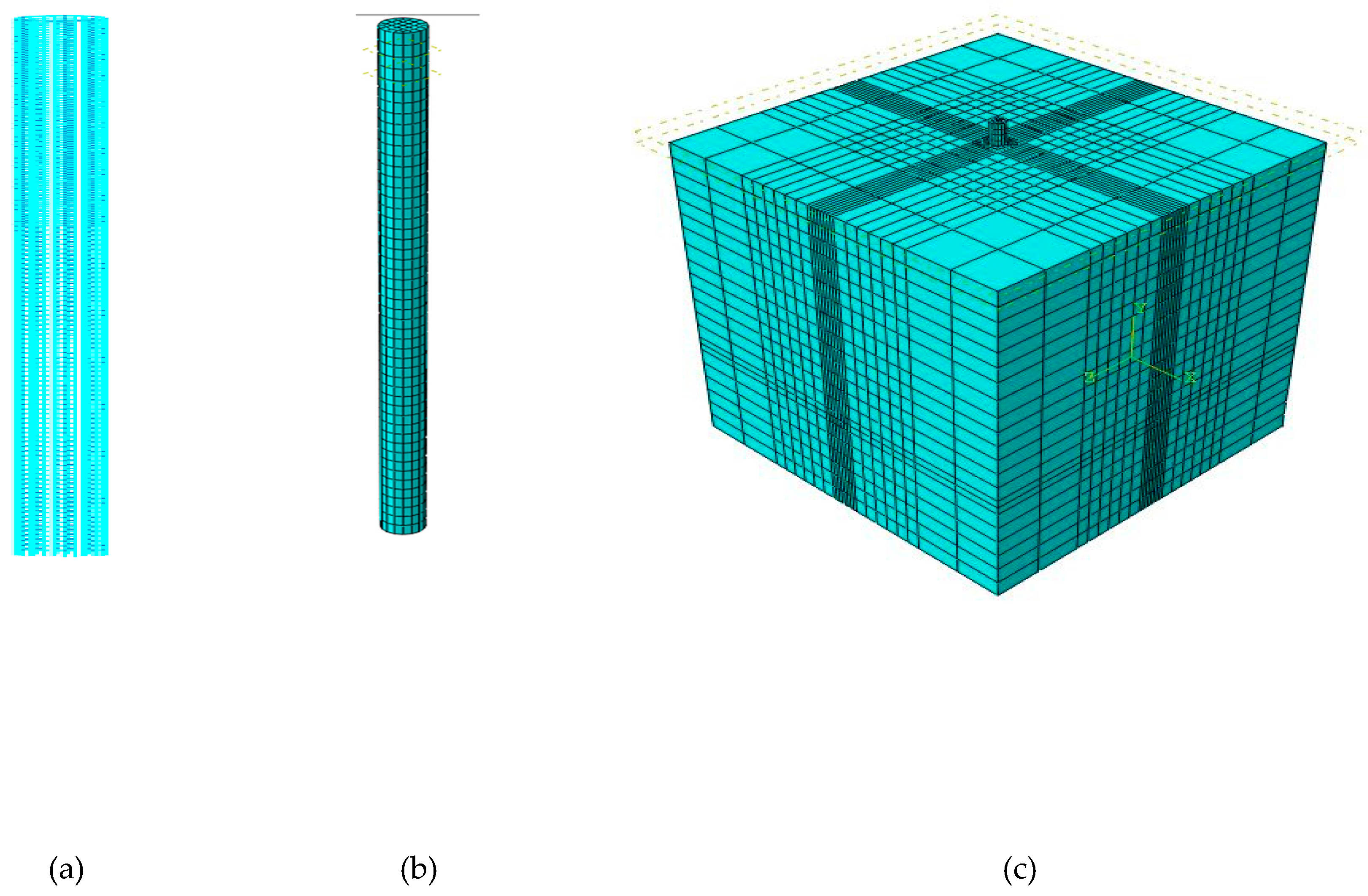
The soil Mesh model has been modeled using 8-node linear brick components with eight reduced integration points (C3D8R). As shown in Figure 6c the mesh size of the surrounding soil and the pile are fine, while the mesh size is coarse, far from the load influence area. The soil material model describes in the previous section is used in modeling the confined soil. The entire geometry of the soil pile has been generated. The crushed stone backfill was modelized mistreatment linear elastoplastic, Mohr-Coulomb failure criteria with non-associated flow rule.
The pile concrete domain was discretized by an 8-node linear brick, reduced integration, hourglass control (C3D8R) elements (Figure 6b). Full interlocking between the sedimentary rock and therefore the soil pile is assumed. In addition, the soil pile sedimentary rock interaction was simulated using two secured master/slave contact surfaces. The 2-Node linear 3-D Truss (T3D2) was used for meshing the steel bar on the pile Figure 6a.
The pile is wholly embedded within the soil, and it is assumed to be also the case concerning the bedrock. Therefore, the entire bearing nodes are taken as fastened, assuming that the soil and pile are entirely warranted. The facet boundaries are constrained against horizontal direction, and the bottom boundaries are constrained against each horizontal and vertical directions. In addition, quiet boundaries are used for wave propagation, and to eliminate the “box effect” (i.e., the reflection of waves back to the model at the boundaries). In order to use the quiet boundaries to the model, infinite components are used at the boundaries.
4. Finite Element Modeling Validation by Field Lateral Loaded Pile Test
4.1. Field Lateral Loaded Pile Testing
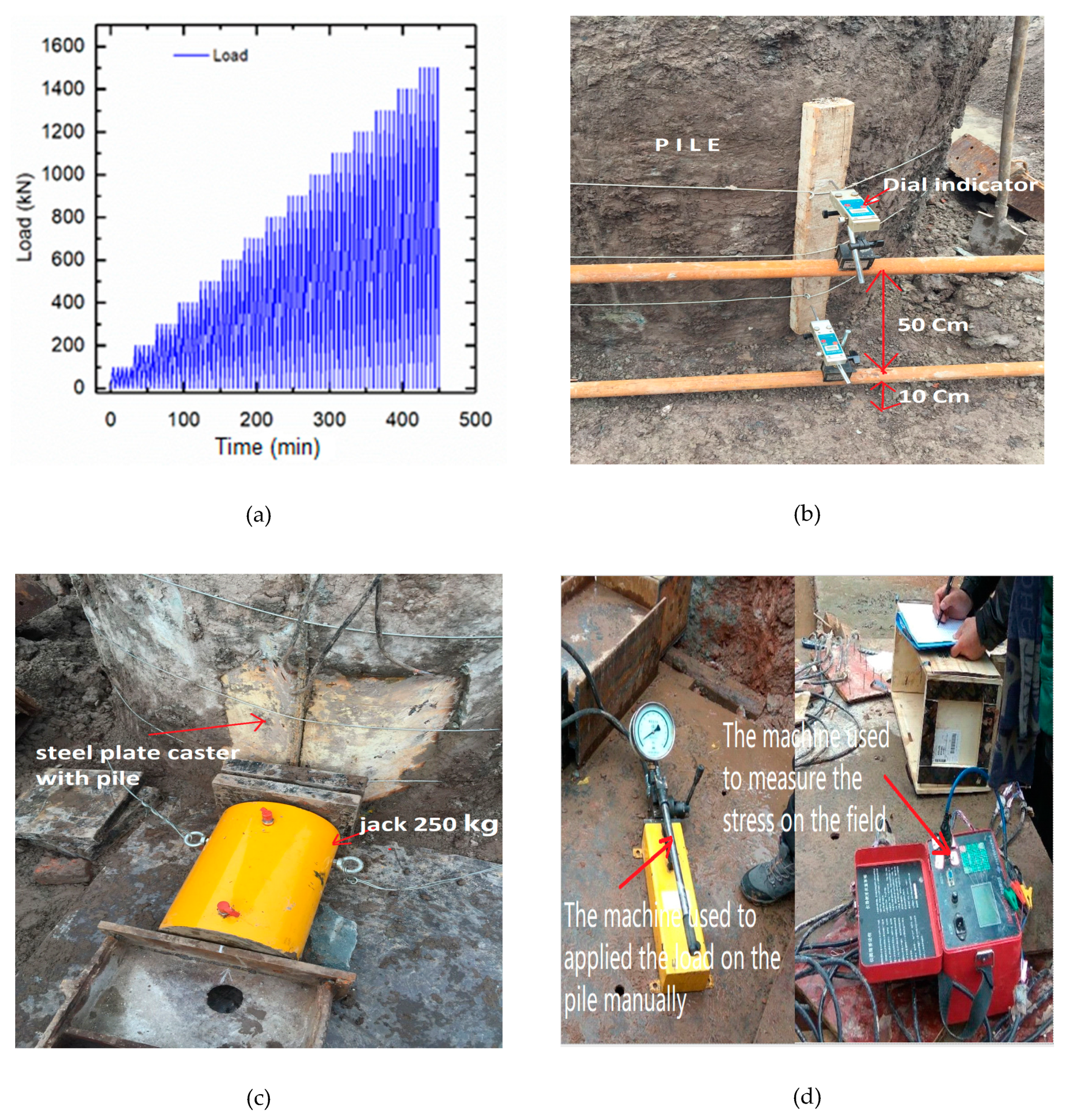
The 22 m piles were embedded into the ground with a diameter of 1.2 m for an overflow of 1.5 m. The piles were poured on the site and hardened for 15 days. The lateral loaded pile test was carried out on a single pile. The soil was composed of several different layers whose characteristics were presented ulterior. A 250 kg jack placed between the two piles is capable of applying a load of up to 300 tons. As shown in Figure 7c, comparators have been laid down, measuring the displacement as a function of lateral load. The load was applied using a manual machine as shown in Figure 7d. The same load applied five times is each time discharged after stabilization of 4 minutes and the unloading will be in rest for 2 min shown in Figure 7a and in Figure 7a shown the pile and the dial indicator used on the side. The same procedure is repeated until the load reaches 1,650,000 N.
4.2. Comparison Between Finte Element Result and Field Measured Data
In this study, a 3D FE modeling was developed to analyze the lateral load behavior of the pile foundation driven into dense sand. The results obtained by the FE analysis were compared with the experimental results determined in lateral load tests on single piles in the different soils and reinforced concrete piles. The analysis aims to validate the planned technique.
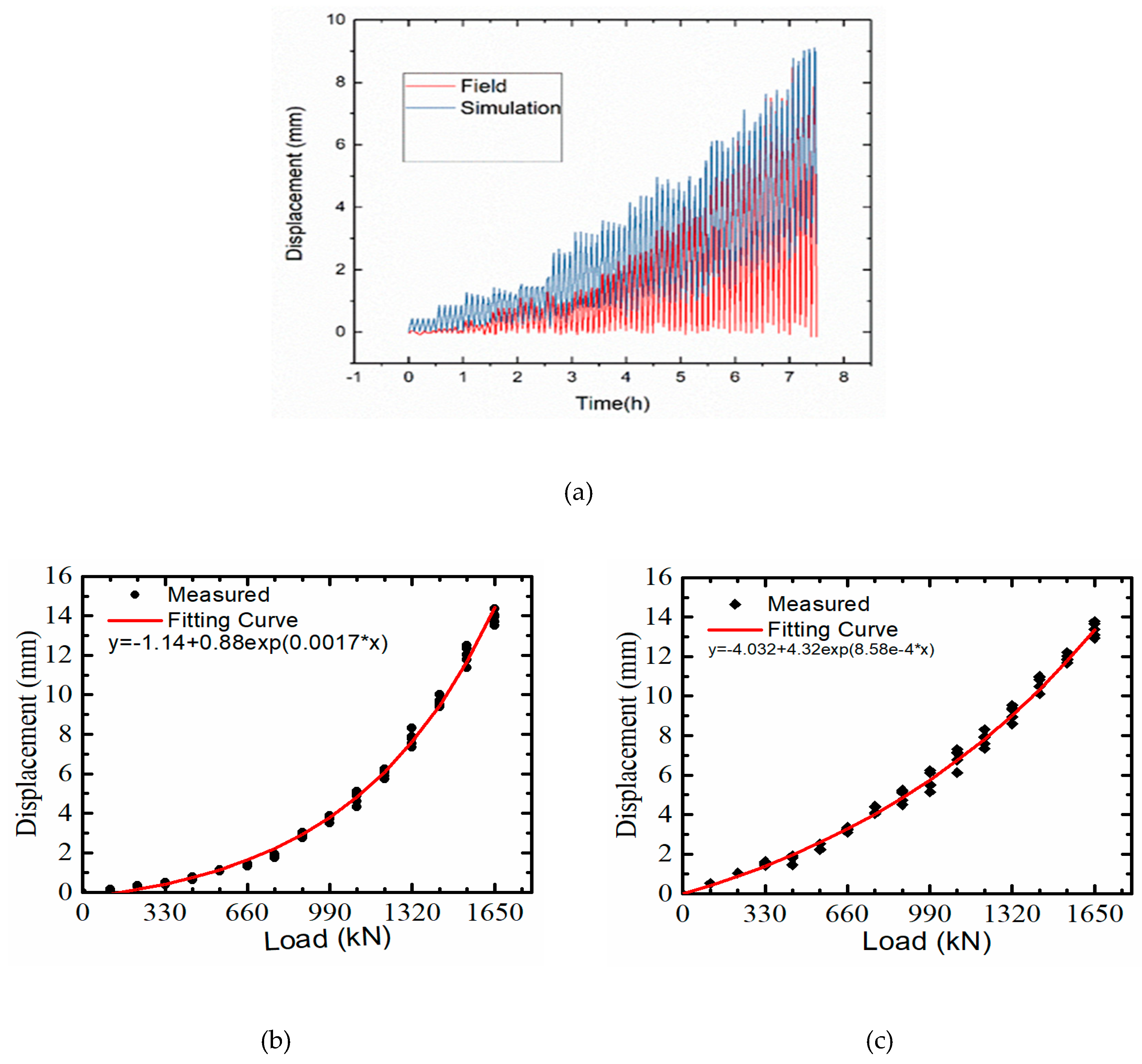
From Figure 8 the simulations show that when applying the load on the pile, the displacement on the curve of the ground is weak at the beginning of the loading (Time (h) between 0 and 1). Then after unloading, the load returns to the original place. However, as the load increases, the curve of the field follows that of the simulation until it reaches. When the load reached a maximum value of 1,650,000 N, the displacement of the RCP taken around the ground surface is about 9.67 mm for the field, while the displacement obtained by FEM is about 9.62 mm. As noted, the difference between the displacement measured under maximum lateral load (1,650,000 N) during the field test and the predicted displacement is less than 1%. This difference could be explained by soil moisture and the condition of applying load on the field. Figure 8 shows the material and pile on the field. Figure 8b and c show the detail of the comparison between the field test and analysis taking at a point on the pile. As shown in Figure 8b and c the pile head displacement of the simulation was 14.79 mm, and the displacement of the pile head on the field was 14.74 mm—a difference of 0.05 mm by applying a different lateral load (110,000N to 1,650,000 N). The relationship between applied lateral load displacements measured at the head of the pile was approximated with the highest precision by the potential exponential functions below (Equation 8) where the parameters y0, A1 and t1 are regression constants.
5. Numerical Results and Analysis
5.1. Lateral Displacement Along the Pile
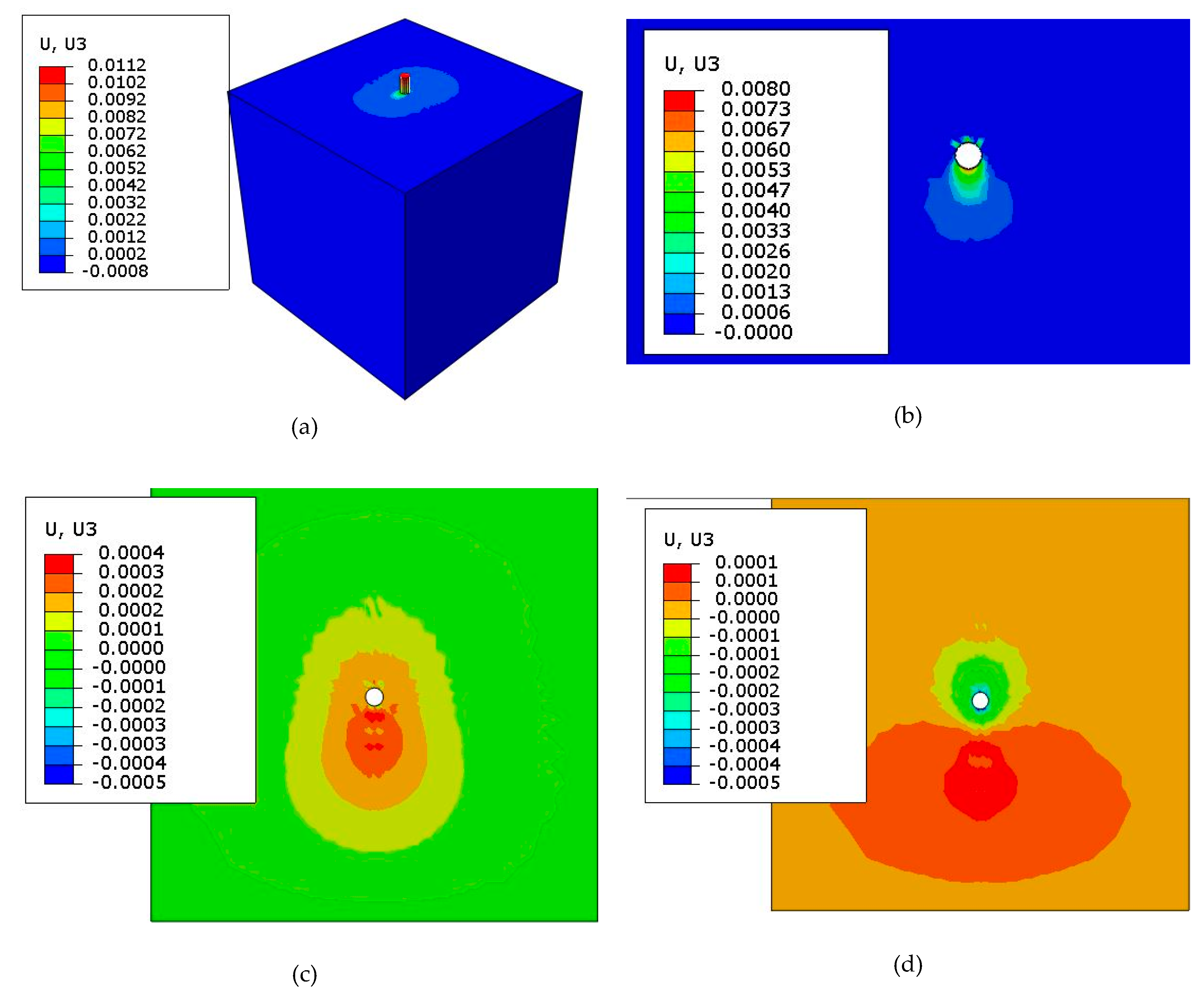
The experiments are carried out on the model of drilled piles considering the self-weight of the pile as a vertical load, unlike the driven pile, which also have the threshing force (driving resistance of the pile). The soil deformation curves vary not only according to the nature of the layers, but also according to the depth by applying the different loads. Therefore, there are several deformation layers, and it can be noted in Figure 9 three layers made by Abaqus™.
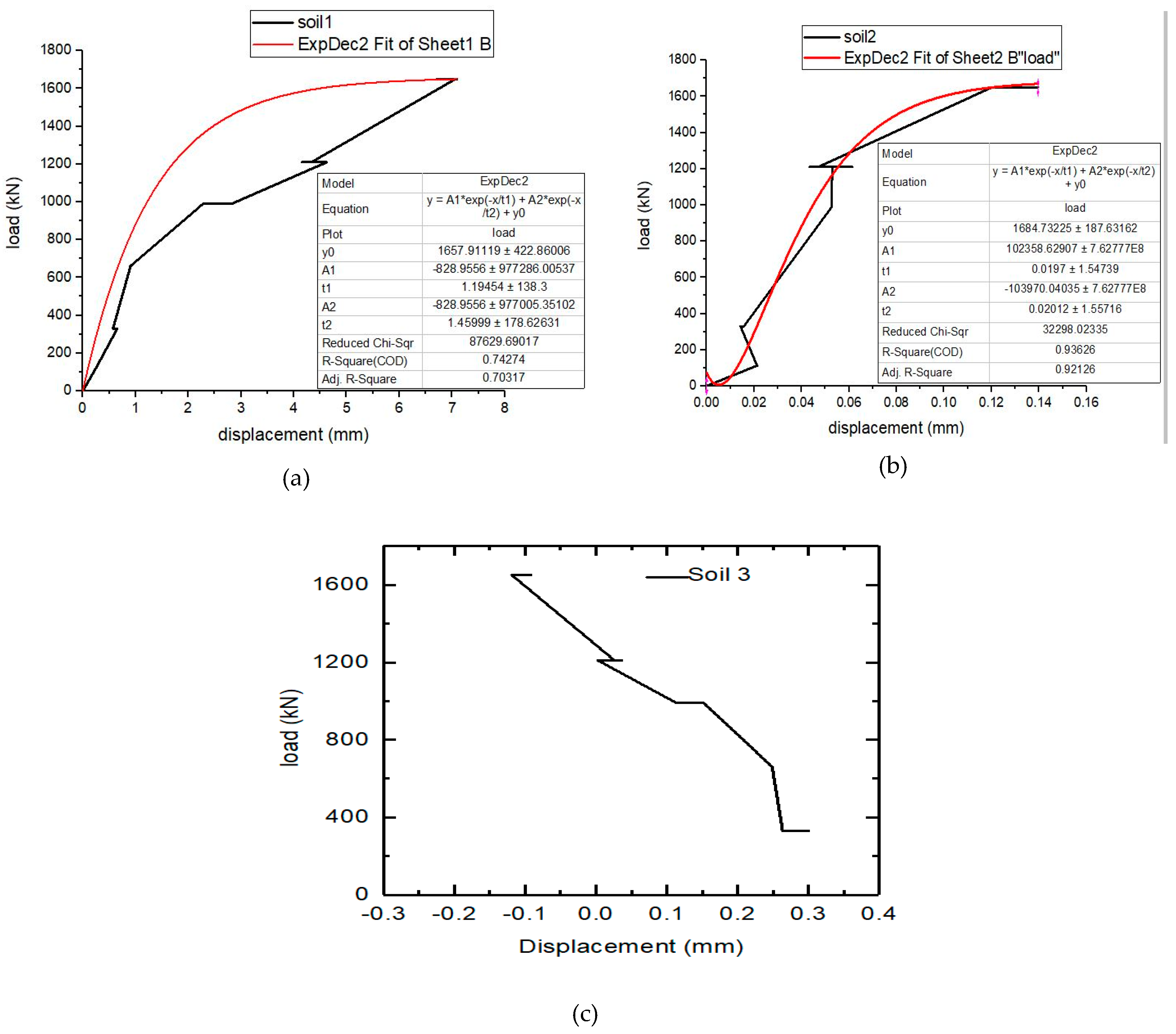
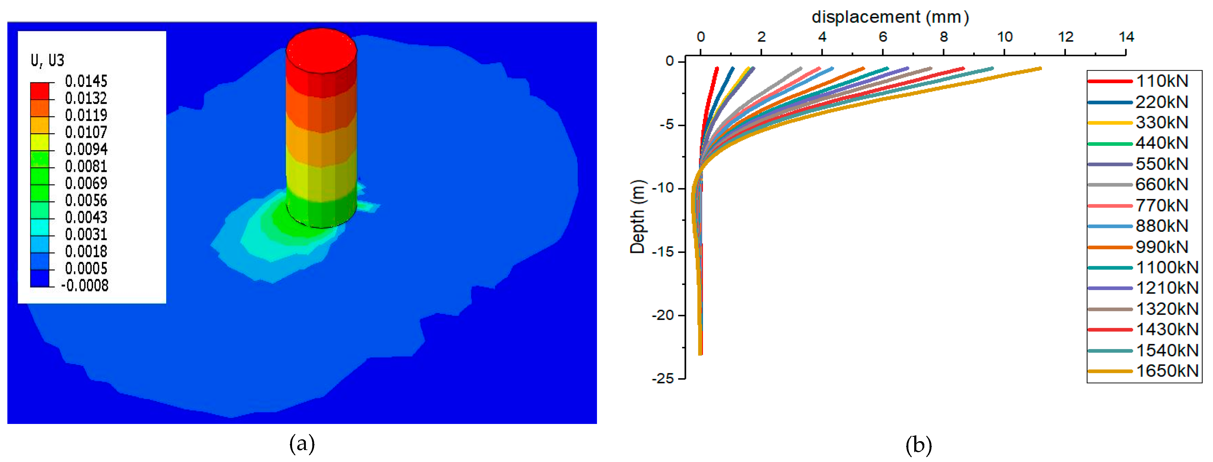
The contours of the ground deform more, once by applying lateral loads (110,000 N to 1,650000 N) of the pile head. The deformation according to the plain view of the soil is represented in Figure 9, while Figure 10 shows the deformation as a function of the different loads applied to the pile in the soil. The deformation is like a wave that propagates in the ground, and which is the epicenter of the pile. However, this wave has strong intensity in the direction of the lateral load applied at the level of the first layers (soil 1 and 2 Figure 10a,b) and strong intensity in the opposite direction of the lateral load applied at the level of the deep layers (soil 3 Figure 10c). The deformations decrease with the depth of the soil. The soil displacement measured at the ground surface around the pile was approximated with the highest precision by the potential exponential functions below (Equation 9) where parameters y0, A1 and t1 are regression constants.
As seen in the Figure 9 U is the spatial displacement at nodes and U3 is the lateral displacement of the pile.
Figure 11a exhibits the FE deformed pile foundation obtained at the load from 110,000 N to 1,650,000 N lateral load. The distribution of piles (Missed equivalent stress), which is shown in Figure 11b by the contour colors, indicating that the reinforced concrete close to the pile head at the first bend region of the pile experiences the very best stress. Figure 11b presents the displacement of lateral deflection generated from the FE model on the pile below different lateral loads. The lateral deformation of the expected pile head at 12.87 mm is applied by the 1,650,000 N load. The pile is inclined within the loading direction. It can be seen that the 3D FE analysis with success captures of the deflection pattern of the pile. Displacement of the field measurements is made at two different points, namely at the head of the pile, and the surrounding of the pile around the ground surface (1.5 m from the head of the pile). One can note that the lateral displacement of the FE model and the field data are almost the same.
5.2. The Stress and strain of Steel Along the Pile
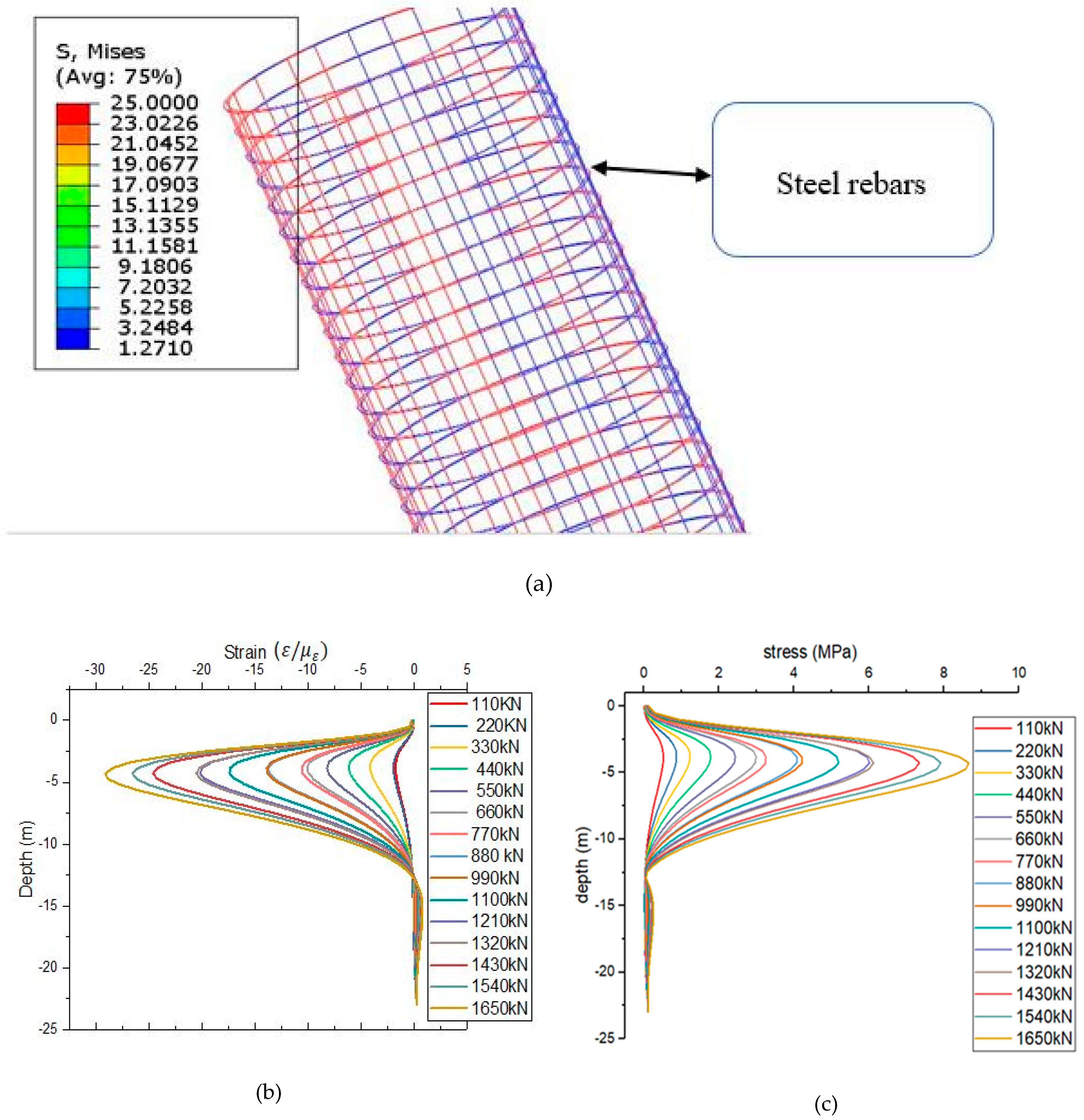
The resistance to longitudinal deformation of the pile is mainly taken up by the reinforcement, which is more resistant in traction than the concrete, which is resistant to compression, hence the usefulness of representing the stress of the reinforcement along the pile depth. The result of the lateral load showing the stress distribution on the pile reinforcement, is that the maximum stress is on 3 to 6 m depth of the pile, and the more the applied lateral load increases, the maximum stress also increases. At a depth of 12.47 m, the minimum positive stresses are found by applying the lateral load of (110,000 N to 1,650,000 N) to the pile head as shown in Figure 12b.
The strain curve is plotted by choosing the same points as the stress along the pile, and is a function of the depth. And it can be observed that the stress and strain are proportional, but opposite in direction from which the maximum strain has a depth of 3 to 6 m of the pile, and the minimum is 12.47 m deep. It is also noted for different lateral loading cases that there is a constant relationship between strain and stress. For example, regarding the loading case of 1,650,000 N, a maximum stress of about 9 MPa is obtained, and a maximum strain of about −30 ε/εμ, which gives a constant value about 3 m of the pile in soil depth. This constant can be justified by the fact that the relationship between these two parameters is Young’s modulus which remains constant for the same material and represents the slope (Hooke’s law).
5.3. Effect of Reinforced Concrete Pile Diameter
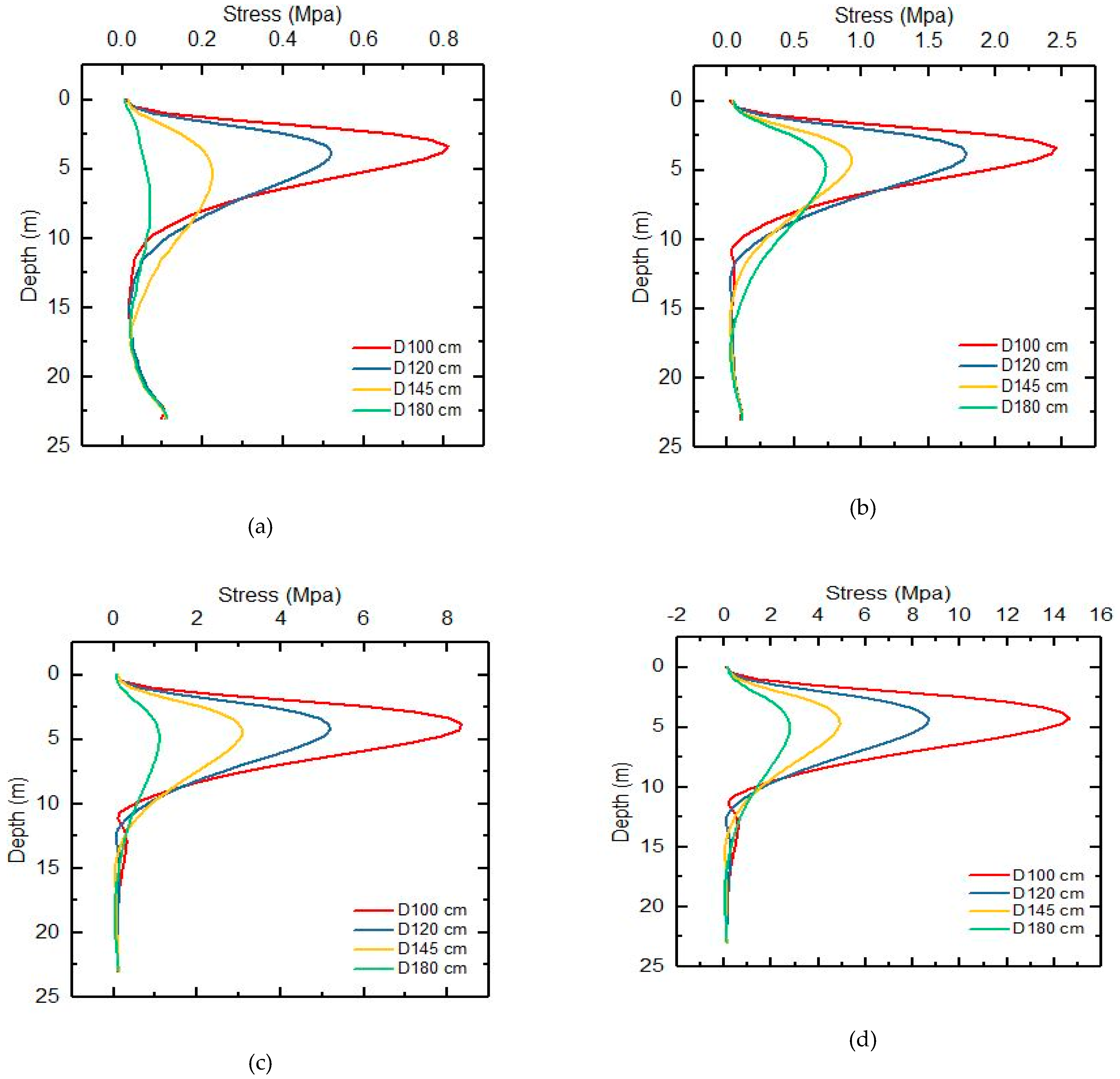
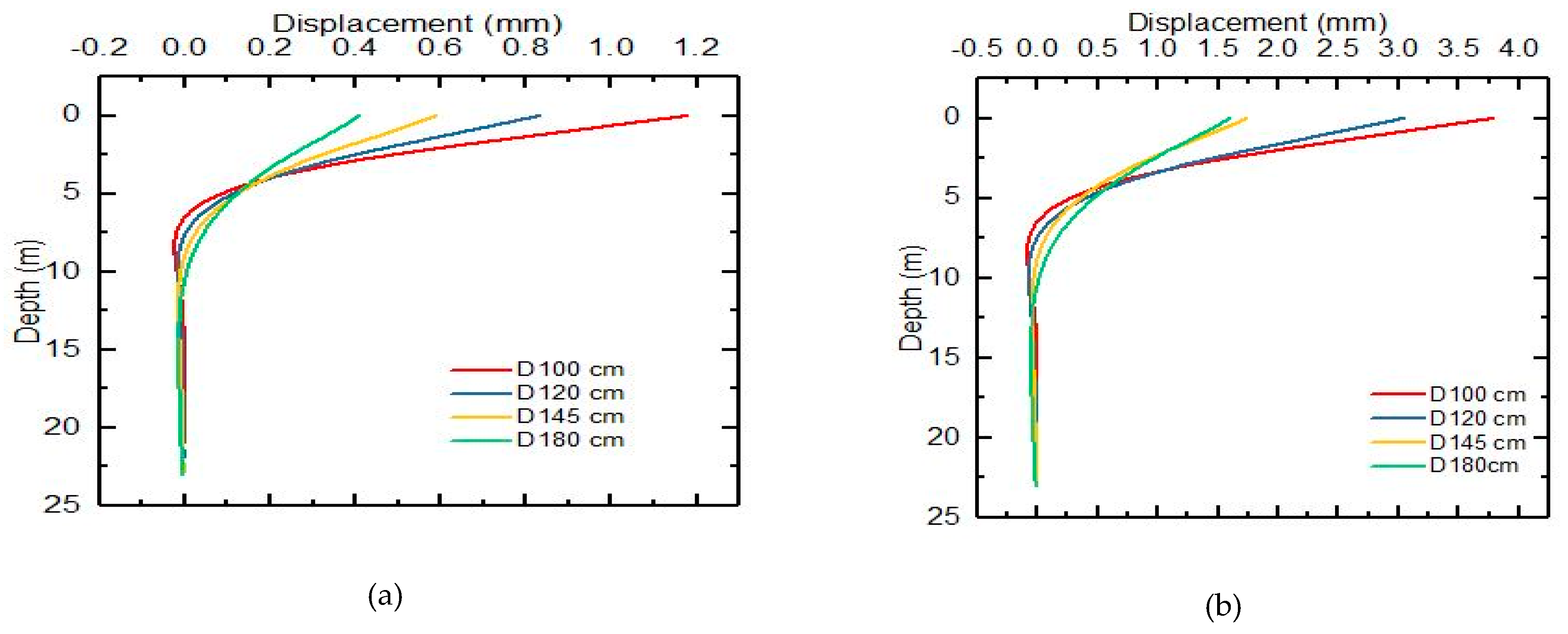
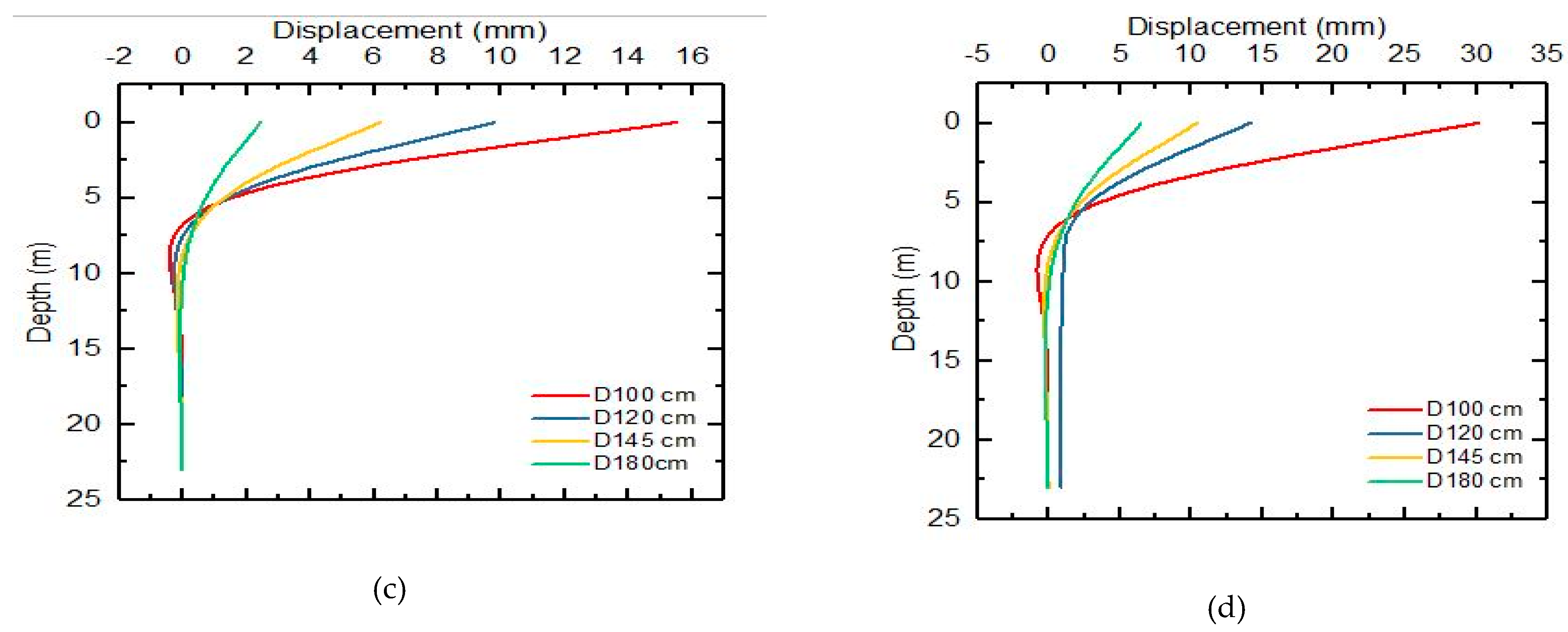
Four different diameters (D = 1.00 m, D = 1.2 m, D = 1.45 m and D = 1.8 m) were chosen to study pile geometry impact at the load (110,000 N, 440,000 N, 1,100,000 N and 1,650,000 N). The pile is supposed to be elastoplastic, and the soil is made using the behavioral relationship of Mohr-Coulomb [1,11,13,15,27,28]. Figure 13 shows the result of pile diameter on the stress distribution on the pile shaft. The increase in pile diameter will increase the pile stiffness, and consequently can decrease the number of tensile stresses on the shaft. The most tensile stress and strain can decrease at a depth move between 4.28 to 4.73 m for a pile diameter of 1.0 to 1.8 m, respectively. The depth of zero tensile stress decreases as the function of the pile diameter is increasing. However, typically, it does not exceed diameters. Once the pile diameter increases, the moment of inertia of its section can increase too, that causes a reduction in stresses (Figure 13) and strain (Figure 14). The lateral displacement distributions in the function of different pile diameters are illustrated in Figure 14. Therefore, a decreasing of the pile shaft systematically has been observed when the pile diameter increases. Once applying the load of 1,650,000 N to the different pile diameters (1.0 m to 1.8 m) the differences between the displacements are perceptible.
For example, the application of 1,650,000 N to pile diameters 1.0 m and 1.2 m cause a slight lateral displacement (decreasing) of the pile shaft from 29.93 mm to 12.57 mm. Thus, the same proportion trend is observed at the level of different loads (110,000 N, 440,000 N, 1,100,000 N, and 1,650,000 N) applied to the different diameters (1.0, 1.20, 1.45, and 1.80 m). Therefore, the displacement decreases when the diameters increase. The linear relationship is developed progressively at different types of soil interface (Figure 14), which will be taken from 2 aspects. Firstly, the loading of the pile shaft can increase non-linearly with the increase in pile diameter that is useful to increase the intervals of the lateral resistance of the pile shaft. Lastly, an enlarged pile diameter expands the pile-soil contact area (linear reaction between pile-soil contact area and pile diameter). As a result of the resistance force between the pile shaft and soil flank, the lateral displacement of soil flank will cause lateral stress and strain on the pile shaft, and thereby a lateral displacement of the pile shaft. Therefore, the ultimate variation law of the lateral displacement of the pile body, that has been used to figure out that between the loadings or lateral friction of piles, takes the dominant role. The loading takes the dominant role during this case.
After analyzing the different curves, it can be noted that, according to the different cases of lateral loads, the stresses are:
- Inversely proportional to diameter (the larger the diameter, the smaller the stress).
- Proportional to the horizontal displacement of the piles (the higher the stress, the greater the horizontal displacement to the pile increases).
- Proportional and opposite direction to the strain (more the stress increases and the more the strain increases, but the direction is negative).
Additionally, the difference between the displacements decreases as shown in Figure 15d. However, the choice of diameter is made by respecting not only the permissible displacement of the piles, which is between (30 and 40 mm), but also to satisfy the financial ratio and the safety factor. The soil is known to be heterogeneous with a significant safety factor which will cover the solicitations due to time, hence the choice to make a comparison between the different types of diameter: D = 100 cm, d = 29, 93 mm, while the displacement of the diameter D = 120 cm, 12, 87 mm.
6. Conclusions
A 3D nonlinear FE model was developed to investigate the performance force of reinforced concrete pile in coherent soil under lateral load. To better understand the mechanical behavior of the whole system, displacement, stress and strain response were calculated along the RCP in the stratified soil, then, there has been generated the conclusion below following the comparison between the RCP simulation carried out by the Mohr-Coulomb model used in Abaqus™, and the field measurement.
- The comparison between the FE simulation result and the field measurement, reveals that at the beginning of the experiment (applied load stage), the displacement of the pile from the field is smaller than the simulation. When the load increases the displacement of the field, and the simulation is almost followed, when the lateral load reached its maximum value of 1,650,000 N the displacement of the field is about 9, 67 mm, while that of the simulation is 9, 62 mm, this great advocate agreement between the FE model and the Field measure.
- The analysis of the influence of the lateral loads level applied on the RCP head shows that the deformation of the soil varies depending on the soil layer. Moreover, it was constant that at a depth of 6m there are the displacement zeros by applying different lateral loads on the pile head (110,000 N to 1,650,000 N).
- It can be concluded that taking a point on the head of the pile, the maximum displacement of the field was 14.74 mm and the displacement of the simulation was 14.79 mm, either 0.05 mm, less than 1 % difference, which is acceptable for validating the simulation.
- It can be noted that taking into account the field and the simulation, the maximum stress and strain on the pile body is at a depth of 5 m and point where the stress and strain are returning to 0 at a depth of 13 m; it can also be noted that stress and strain have opposite directions.
Author Contributions
Conceptualization, T.Y. (Touré Youssouf) and T.Y. (Tianlai Yu); Methodology, T.Y. (Touré Youssouf); Software, A.O.C.; Validation, T.Y. (Touré Youssouf), T.Y. (Tianlai Yu), D.A. and D.Y.; Formal Analysis, Conceptualization, T.Y. (Touré Youssouf); Investigation, D.A; Resources, T.Y. (Touré Youssouf); Data Curation, D.Y.; Writing—Original Draft Preparation, T.Y. (Touré Youssouf); Writing—Review & Editing, T.Y. (Touré Youssouf), A.O.C.; Visualization T.Y. (Touré Youssouf); Supervision, T.Y. (Tianlai Yu).
Funding
This work is supported by Heilongjiang Transport Technology Project Grant no. 2014013.
Acknowledgments
The author would like to thank the Northeast Forestry University Forest and his supervisor for valuable suggestion to facilitate this project. Also, extend his gratitude to the Chinese Government converted by Northeast Forestry University and particularly all members of the department of civil engineering. Additionally, we are also grateful to the reviewers and co-editor for their valuable comments and suggestions for this paper.
Conflicts of Interest
The author declares no conflict of interest.
References
- Kourkoulis, R.; Gelagoti, F.; Anastasopoulos, I.; Gazetas, G. Slope Stabilizing Piles and Pile-Groups: Parametric Study and Design Insights. J. Geotech. Geoenviron. Eng. 2011, 137, 663–677. [Google Scholar] [CrossRef]
- Di Laora, R.; Maiorano, R.M.S.; Aversa, S. Ultimate Lateral Load Of Slope-Stabilising Piles. Geotech. Lett. 2017, 7, 2045–2543. [Google Scholar] [CrossRef]
- Mujah, D.; Ahmad, F.; Hazarika, H.; Watanabe, N. The Design Method of Slope Stabilizing Piles: A Review. Int. J. Curr. Eng. Technol. 2013, 3, 224–229. [Google Scholar]
- Jain, A.; Gupta, T.; Sharma, R.K. Measurement and Repair Techniques of Corroded Underwater Piles: An Overview. Int. J. Eng. Res. Appl. 2016, 6, 19–27. [Google Scholar]
- Cai, Y.; Tu, B.; Yu, J.; Zhu, Y.; Zhou, J. Numerical Simulation Study on Lateral Displacement of Pile Foundation and Construction Process Under Stacking Loads. Complexity 2018, 2018, 2128383. [Google Scholar] [CrossRef]
- Mardfekri, M.; Gardoni, P.; Roesset, J.M. Modeling Laterally Loaded Single Piles Accounting for Nonlinear Soil-Pile Interactions. J. Eng. 2013, 2013, 243179. [Google Scholar] [CrossRef]
- Kavitha, P.; Venkatesh, M.M.; Sundaravadivelu, R. Soil-Structure Interaction Analysis of a Dry Dock. Aquat. Procedia 2015, 4, 287–294. [Google Scholar] [CrossRef]
- Salman, F.A.; Mohammed, M.M.; Shirazi, S.M.; Jameel, M. Reinforcement in Concrete Piles Embedded in Sand. Int. J. Phys. Sci. 2010, 5, 2259–2271. [Google Scholar]
- Hashem-Ali, S.F. Analytical Methods for Predicting Load-Displacement Behaviour of Piles; Durham E-Theses, Durham University: Durham, UK, 2014. [Google Scholar]
- Sections, C. Analysis Methods for Laterally Loaded Pile Groups Using an Advanced Modeling of Reinforced Concrete Sections. Materials 2018, 11, 300. [Google Scholar]
- Kontoni, D.-P.; Farghaly, A. 3d Fem Analysis of a Pile-Supported Riverine Platform under Environmental Loads Incorporating Soil-Pile Interaction. Computation 2018, 6, 8. [Google Scholar] [CrossRef]
- Cui, K.; Feng, J.; Zhu, C. A Study on the Mechanisms of Interaction between Deep Foundation Pits and The Pile Foundations of Adjacent Skewed Arches as Well as Methods for Deformation Control. Complexity 2018, 2018, 6535123. [Google Scholar] [CrossRef]
- Abdel-Rahman, K.; Achmus, M. Numerical Modelling of Combined Axial and Lateral Loading of Vertical Piles. In Numerical Methods in Geotechnical Engineering, Proceedings of the 6th Eur. Conferences, Denver, CO, USA, 5–8 August 2000; American Society of Civil Engineers: New York, NY, USA, 2006; pp. 575–581. [Google Scholar]
- Kim, B.T.; Yoon, G.L. Laboratory Modeling of Laterally Loaded Pile Groups in Sand. KSCE J. Civ. Eng. 2011, 15, 65–75. [Google Scholar] [CrossRef]
- Shaia, H.A.; Abbas, S.A. Three-Dimensional Analysis Response of Pile Subjected to Oblique Loads. Int. J. Sci. Eng. Res. 2015, 6, 508–511. [Google Scholar]
- Abdel-Mohti, A.; Khodair, Y. Analytical Investigation of Pile-Soil Interaction in Sand under Axial and Lateral Loads. Int. J. Adv. Struct. Eng. 2014, 6, 54. [Google Scholar] [CrossRef]
- Phanikanth, V.S.; Choudhury, D.; Reddy, G.R. Response of Single Pile under Lateral Loads in Cohesionless Soils. Electron. J. Geotech. Eng. 2010, 15, 813–830. [Google Scholar]
- Fuentes, J.L.; Gamble, W.L. Design, Manufacture, and Installation of Concrete Piles; ACI 543r-00; ACI Committee: Bismarck, ND, USA, 2005; pp. 1–49. [Google Scholar]
- Schall, J.D.; Price, G.R. National Cooperative Highway Research Program: Report 515, 2004.
- Kanakeswararao, T.; Ganesh, B. “Analysis of Pile Foundation Subjected to Lateral and Vertical Loads,”. Int. J. Eng. Trends Technol. no. 2. 2017, 113–127. [Google Scholar] [CrossRef]
- Niyaz, A.A.; Junaid, A.; Shafeeque, A.; Mohd, B.; Sadique, A.; Noor, K.A. Pile-Soil Interaction by Finite. pp. 2016–2017. Available online: https://pdfs.semanticscholar.org/1077/2e22206003382ea499c3e7978211343be406.pdf (accessed on 28 March 2019).
- Balendra, S. Numerical Modeling of Dynamic Soil-Pile-Structure Interaction. MSc Thesis, Department of Civil and Environmental Engineering, Washington State University, Washington, DC, USA, December 2005. [Google Scholar]
- Salman, F.A.; Fattah, M.Y.; Mohammed, M.M.; Hashim, R. Numerical Investigation on Reinforcement Requirement for Piles Embedded in Clay. Sci. Res. Essays 2010, 5, 2731–2741. [Google Scholar]
- Brown, D.A.; O’Neill, M.W.; Hoit, M.; Mcvay, M.; el Naggar, M.H.; Chakraborty, S. Static and Dynamic Lateral Loading of Pile Groups. Natl. Coop. Highw. Res. Progr. 2001, 461, 50. [Google Scholar]
- Rasmussen, L.; Wolf, K.; Bo, L.; Rasmussen, K.L. A Literature Study on the Effects of Cyclic Lateral Loading of Monopiles in Cohesionless Soils; Aalborg University: Aalborg, Denmark, 2013. [Google Scholar]
- Favaretti, C. Towards Next Generation P-Y Relationships: Part 1 Report Part 1: State of Practice–State of the Art; University of California: Irvine, CA, USA, 2018. [Google Scholar]
- Wrana, B. Pile Load Capacity–Calculation Methods. Stud. Geotech. Mech. 2015, 37, 4. [Google Scholar] [CrossRef]
- Ashour, M.; Norris, G. Pile Group Program for Full Material Modeling and Progressive Failure; The Final Report; California Department of Transportation: Sacramento, CA, USA, 2008. [Google Scholar]
- Dodds, A.; Martin, G. Modeling Pile Behavior in Large Pile Groups under Lateral Loading. 2007. Available online: https://www.researchgate.net/profile/Cihan_Akdag/publication/265592075_AN_INVESTIGATION_OF_THE_BEHAVIOR_OF_FIBER_REINFORCED_CONCRETE_PILES_UNDER_LATERAL_LOADING /links/5412eb840cf2788c4b3587e7/AN-INVESTIGATION-OF-THE-BEHAVIOR-OF-FIBER-REINFORCED-CONCRETE-PILES-UNDER-LATERAL-LOADING.pdf (accessed on 28 March 2019).
- Graduate School of Natural and Applied Sciences an Investigation of the Behavior of Fiber Reinforced Concrete Piles under an Investigation of The Behavior Of. 2011.
- Johnson, K.; Lemcke, P.; Karunasena, W.; Sivakugan, N. Modelling the Load E Deformation Response of Deep Foundations under Oblique Loading. Environ. Model. Softw. 2006, 21, 1375–1380. [Google Scholar] [CrossRef]
- Hazzar, L.; Hussien, M.N.; Karray, M. Influence of Vertical Loads on Lateral Response of Pile Foundations in Sands and Clays. J. Rock Mech. Geotech. Eng. 2017, 9, 291–304. [Google Scholar] [CrossRef]
- Rahemi, N. Numerical Investigation on Lateral Deflection of Single Pile under Static and Dynamic Loading. Master’s Thesis, Eastern Mediterranean University, Famagusta, Turkey, 2012. [Google Scholar]
- Bahloul, D.; Moussai2, B. Three-Dimensional Analysis of Laterally Loaded Barrette Foundation Using Plaxis 3d. Tanda Kardinal Pemeriksaan Eksternal Jenasah Diduga Tenggelam Dari Data Bagian Ilmu Kedokt. Forensik Rsup Sanglah Bali Tahun 2012–2014. 2015, 4, pp. 29–42. Available online: http://www.eventscribe.com/2016/CECAR7/assets/pdf/326516.pdf (accessed on 28 March 2019).
- El Naggar, M.H.; Bentley, K.J. Dynamic Analysis for Laterally Loaded Piles and Dynamic P-Y Curves. Can. Geotech. J. 2000, 37, 1166–1183. [Google Scholar] [CrossRef]
- Bentley, K.J.; el Naggar, M.H. Numerical Analysis of Kinematic Response of Single Piles. Can. Geotech. J. 2000, 37, 1368–1382. [Google Scholar] [CrossRef]
- Heidari, M.; Jahanandish, M.; el Naggar, H.; Ghahramani, A. Nonlinear Cyclic Behavior of Laterally Loaded Pile in Cohesive Soil. Can. Geotech. J. 2014, 51, 129–143. [Google Scholar] [CrossRef]
- Rahmani, A.; Taiebat, M.; Finn, W.; Ventura, C. “Evaluation of p-y Curves Used in Practice for Seismic Analysis of Soil-Pile Interaction,”. GeoCongress 2012, vol. 10.1061/97, no. May. 1780–1788. [Google Scholar]
- Zhan, Y.G.; Wang, H.; Liu, F.C. Modeling Vertical Bearing Capacity of Pile Foundation by Using Abaqus. Electron. J. Geotech. Eng. 2012, 17, 1855–1865. [Google Scholar]
- Qu, H. Hysteresis Analysis on Beam-Column Connection of Concrete-Filled Steel Tubular Structure under Cyclic Loading. Trans. Tech. Publ. Switz. Mater. 2012, 517, 376–381. [Google Scholar] [CrossRef]
- Najafgholipour, M.A.; Dehghan, S.; Dooshabi, A.; Niroomandi, A. Finite Element Analysis of Reinforced Concrete Beam-Column Connections With Governing Joint Shear Failure Mode. Lat. Am. J. Solids Struct. 2017, 14, 1200–1225. [Google Scholar] [CrossRef]
- Voyiadjis, G.; Taqieddin, Z. Elastic-Plastic and Damage Model for Concrete Materials: Part I-Theoretical Formulation. Int. J. Struct. Chang. Solids 2009, 1, 31–59. [Google Scholar]
- Asadi, M. Experimental Test and Finite Element Modelling of Pedestrian. Test, No. Figure 1. 2010; 60876. [Google Scholar]
- Maheshwari, B.K.; Truman, K.Z.; el Naggar, M.H.; Gould, P.L. Three-Dimensional Finite Element Nonlinear Dynamic Analysis of Pile Groups for Lateral Transient and Seismic Excitations. Can. Geotech. J. 2004, 41, 118–133. Available online: https://0-scholar-google-com.brum.beds.ac.uk/scholar?q=Parameterised+Finite+Element+Modelling+of+RC+Beam+Shear+Failure&hl=fr&as_sdt=0&as_vis=1&oi=scholart (accessed on 28 March 2019). [CrossRef]
- Budge, S. Design And Analysis of Driven Pile Foundations for Lateral Capacity of Single Piles.
Figure 1.
The geo-localization of the Yanchuan Bridge. (a)the Yanji city locate in china, (b) location of construction at Yanji city, (c) construction view of the bridge, (d) view of the pile test.
Figure 1.
The geo-localization of the Yanchuan Bridge. (a)the Yanji city locate in china, (b) location of construction at Yanji city, (c) construction view of the bridge, (d) view of the pile test.

Figure 2.
The deflection, rotation, moment, shear force and soil resistance of the pile foundation around the pile.
Figure 2.
The deflection, rotation, moment, shear force and soil resistance of the pile foundation around the pile.

Figure 3.
Mohr-Coulomb failure criterion.

Figure 4.
Modeling of the steel used for analysis the pile, (a) the detail of rebar used in Abaqus™, (b) Cover and reinforcement of the pile in which the concrete would be poured.
Figure 4.
Modeling of the steel used for analysis the pile, (a) the detail of rebar used in Abaqus™, (b) Cover and reinforcement of the pile in which the concrete would be poured.

Figure 5.
Soil-pile interface modeling in Abaqus™ (a) No sliding, (b) Sliding.

Figure 6.
The meshing modeling of the soil pile (a) Steel bar; (b) Reinforcement Concrete Pile (RCP); (c) assembly with meshing.
Figure 6.
The meshing modeling of the soil pile (a) Steel bar; (b) Reinforcement Concrete Pile (RCP); (c) assembly with meshing.

Figure 7.
The material used on the field to the test; (a) The modeling of applying a load on the pile head; (b) The pile; (c) The view of the jack; (d) The machines used to apply load and measure the stress and strain.
Figure 7.
The material used on the field to the test; (a) The modeling of applying a load on the pile head; (b) The pile; (c) The view of the jack; (d) The machines used to apply load and measure the stress and strain.

Figure 8.
Comparison of lateral displacement between Field measurement and Finale Element (FE) Simulation result; (a) (H-t-Y0) the curve at the point of the ground surface test pile force FE Simulation result and field result; (b) Field measurement at the pile head; (c) FE Simulation result at the pile head.

Figure 9.
Plan view of Soil deformation at different depth under lateral loading; (a) Soil deformation on the lateral load; (b) Top of the first layer; (c) Top of the Second Layer; (d) Top Third Layer.
Figure 9.
Plan view of Soil deformation at different depth under lateral loading; (a) Soil deformation on the lateral load; (b) Top of the first layer; (c) Top of the Second Layer; (d) Top Third Layer.

Figure 10.
The relation of the first two soil displacement and the lateral load applying on the pile; (a) FE Simulation result for the soil 1; (b) FE Simulation result for the soil 2; (c) FE Simulation result for the soil 3.
Figure 10.
The relation of the first two soil displacement and the lateral load applying on the pile; (a) FE Simulation result for the soil 1; (b) FE Simulation result for the soil 2; (c) FE Simulation result for the soil 3.

Figure 11.
The displacement of the lateral load on the pile head; (a) Lateral deformation of piles; (b) Lateral deformation profiles.
Figure 11.
The displacement of the lateral load on the pile head; (a) Lateral deformation of piles; (b) Lateral deformation profiles.

Figure 12.
Stress and strain of a lateral load of steel along the pile; (a) the steel bar modeling; (b) the strain of lateral of steel along the pile; (c) the stress of lateral of steel along the pile.
Figure 12.
Stress and strain of a lateral load of steel along the pile; (a) the steel bar modeling; (b) the strain of lateral of steel along the pile; (c) the stress of lateral of steel along the pile.

Figure 13.
Impact of diameter on the stress distribution along of reinforced concrete pile; (a) The stress of the pile in the function of different diameters at load 110,000 N; (b) The stress of the pile in the function of different diameters at load 440,000 N; (c) The stress of the pile in the function of different diameters at load 1,100,000 N; (d) The stress of the pile in the function of different diameters at load 1,650,000 N.

Figure 14.
Impact of diameter on the strain distribution along the reinforced concrete pile, (a) The strain of the pile in the function of different diameters at load 110,000 N; (b) The strain of the pile in the function of different diameters at load 440,000 N; (c) The strain of the pile in the function different of diameters at load 1,100,000 N; (d) The strain of the pile in the function of different diameters at load 1,650,000 N.

Figure 15.
Impact of diameter on the displacement distribution along of reinforced concrete pile; (a) The displacement of the pile in the function of different diameters at load 110,000 N; (b) The displacement of the pile in the function of different diameters at load 440,000 N; (c) The displacement of the pile in the function of different diameters at load 1,100,000 N; (d) The displacement of the pile in the function of different diameters at load 1,650,000 N.


Table 1.
Geotechnical properties of the soil.
| Soil | Elasticity | Mohr-Coulomb | |||||
|---|---|---|---|---|---|---|---|
| Quality | Layer Thickness | Young’s Modulus (Pa) | Poison Ratio | Density (kg/m3) | Friction Angle (°) | Cohesion (KPa) | |
| Heavy weathered sandstone | top | 6.5 | 76.80 × 10 e6 | 0.25 | 1650 | 25.32 | 34 |
| Second | 3.1 | 56.50 × 10 e6 | 0.25 | 1850 | 28.30 | 2.57 | |
| third | 3.2 | 96.70 × 10 e6 | 0.25 | 1690 | 23.18 | 2.2 | |
| fourth | 0.8 | 57.80 × 10 e6 | 0.25 | 1675 | 26.77 | 2.8 | |
| Metamorphic siltstone mudstone | fifth | 8.4 | 64.20 × 10 e6 | 0.25 | 1600 | 22.24 | 4.6 |
Institute of Geological Investigation of the Province of Jilin in China.
Table 2.
The characteristic of Pile Concrete.
| Pile Concrete | ||
|---|---|---|
| Density | 2500 | |
| Elastic | Young’s Modulus (Pa) | Poisson’s Ratio |
| 30•1010 | 0.3 | |
Table 3.
The characteristic of Pile steel.
| Steel for the Pile | |||||
|---|---|---|---|---|---|
| Density (kg/m3) | 7800 | ||||
| Elastic | Young’s Modulus (Pa) | Poisson´s Ratio | |||
| 21e11 | 0.2 | ||||
| Concrete damage plasticity | Dilatation Angle (°) | Eccentricity | fbo/fco | k | Viscosity parameter |
| 31 | 0.1 | 1.16 | 0.6677 | 0 | |
Table 4.
Interaction parameters.
| Properties Chosen for Model | Alternative Option | |
|---|---|---|
| Interaction | Mechanical contact<surface to surface> | <Node to surface> |
| Theory model | Frictional behavior contacts by Mohr-coulomb theory | Various |
| Sliding formulation | Small sliding | Finite sliding |
| Interaction properties | ||
| Tangential behavior | ||
| Friction formation | Penalty friction | Various |
| Friction coefficient (–) | 0.75 | 0.5 |
| Shear stress limit | No | Option limit can be set |
| Elastic slip, Absolute distance [m] | 0.001 | 0.0005 |
| Normal behavior, hard contact with penalty constraint method | ||
| Separation after contact | Allowed | Not allowed |
| Tie contact for the tip of the pile | Assigned |
© 2019 by the authors. Licensee MDPI, Basel, Switzerland. This article is an open access article distributed under the terms and conditions of the Creative Commons Attribution (CC BY) license (http://creativecommons.org/licenses/by/4.0/).
Share and Cite
MDPI and ACS Style
Youssouf, T.; Yu, T.; Abdramane, D.; Cyriaque, A.O.; Youssouf, D. Force Performance Analysis of Pile Behavior of the Lateral Load. Infrastructures 2019, 4, 13. https://0-doi-org.brum.beds.ac.uk/10.3390/infrastructures4020013
AMA Style
Youssouf T, Yu T, Abdramane D, Cyriaque AO, Youssouf D. Force Performance Analysis of Pile Behavior of the Lateral Load. Infrastructures. 2019; 4(2):13. https://0-doi-org.brum.beds.ac.uk/10.3390/infrastructures4020013
Chicago/Turabian StyleYoussouf, Touré, Tianlai Yu, Dembélé Abdramane, Assogba Ogoubi Cyriaque, and Diakité Youssouf. 2019. "Force Performance Analysis of Pile Behavior of the Lateral Load" Infrastructures 4, no. 2: 13. https://0-doi-org.brum.beds.ac.uk/10.3390/infrastructures4020013