On the Use of Ensemble Empirical Mode Decomposition for the Identification of Bridge Frequency from the Responses Measured in a Passing Vehicle


Abstract
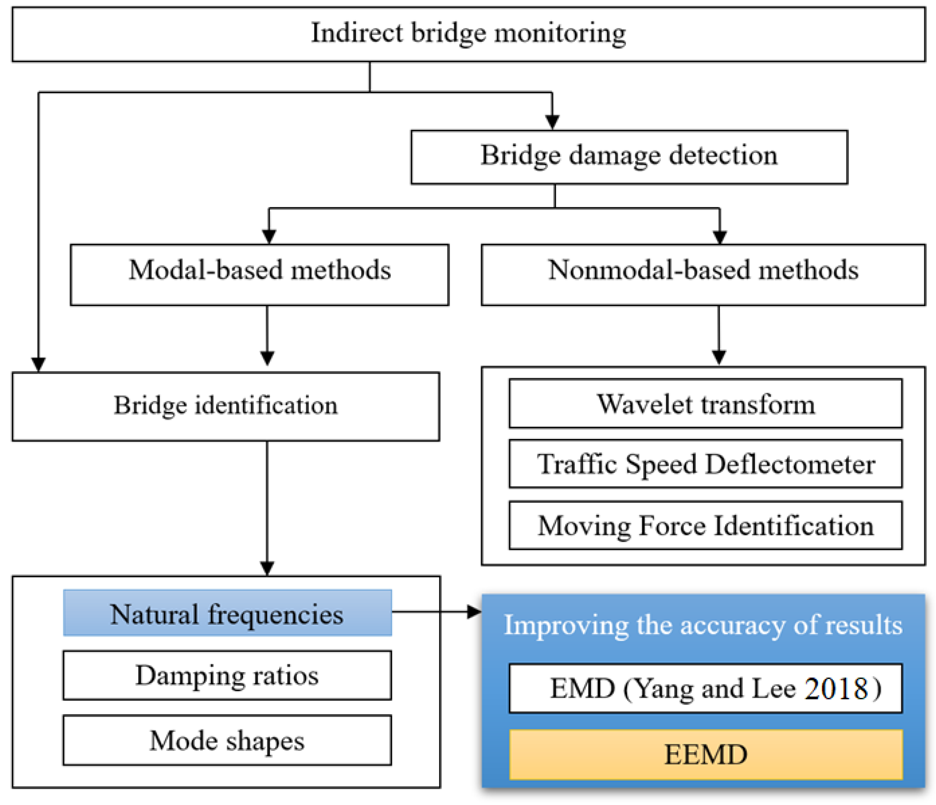
:1. Introduction
2. Theoretical Background
2.1. Empirical Mode Decomposition (EMD) Method
- (a)
- Obtain the original signal;
- (b)
- Identify the positive peaks and negative peaks of the original signal; the upper envelope and the lower envelope can be obtained as connecting maxima and minima of the original signal with the cubic spline separately. Then, the mean value of upper envelop and the lower envelop can be calculated;
- (c)
- Subtract the mean from the original signal to obtain the first intrinsic mode function (IMF1);
- (d)
- The first residual component is calculated by subtracting IMF1 from the original signal. This residual component is treated as a new data and subjected to the same process described above to calculate the next IMF.
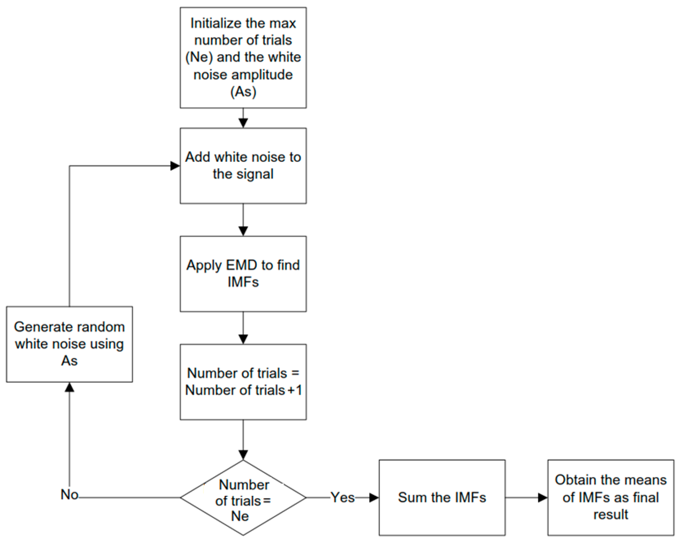
2.2. Ensemble Empirical Mode Decomposition (EEMD) Method
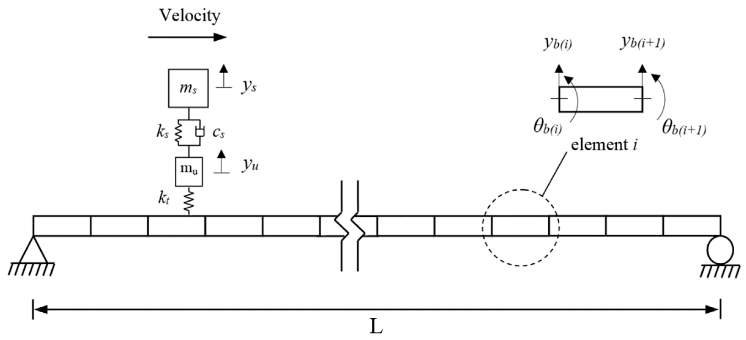
3. Numerical Modelling of Vehicle Bridge Interaction
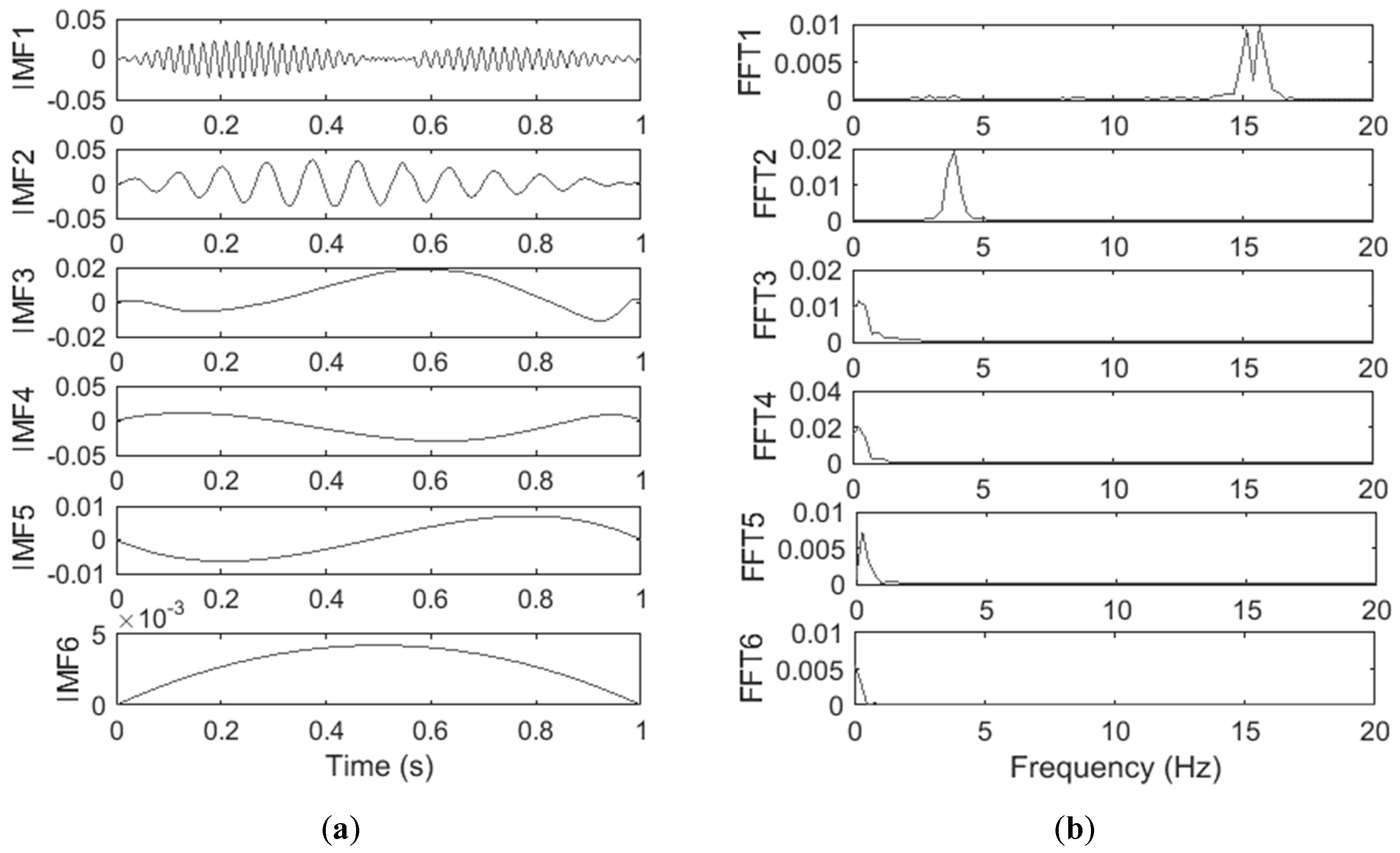
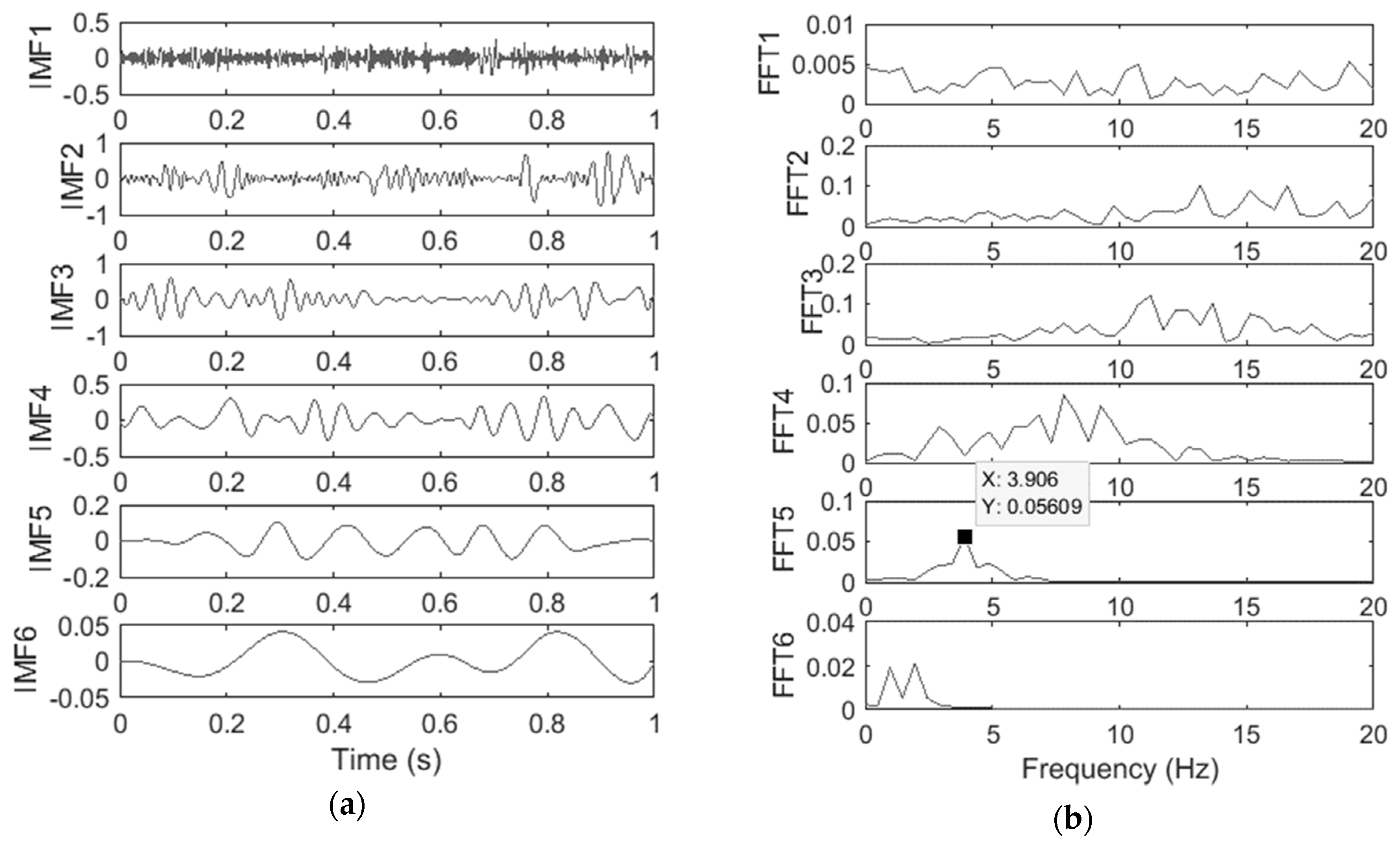
4. Estimation of the Bridge Frequency Using the EMD Method
4.1. Effect of Road Surface Roughness
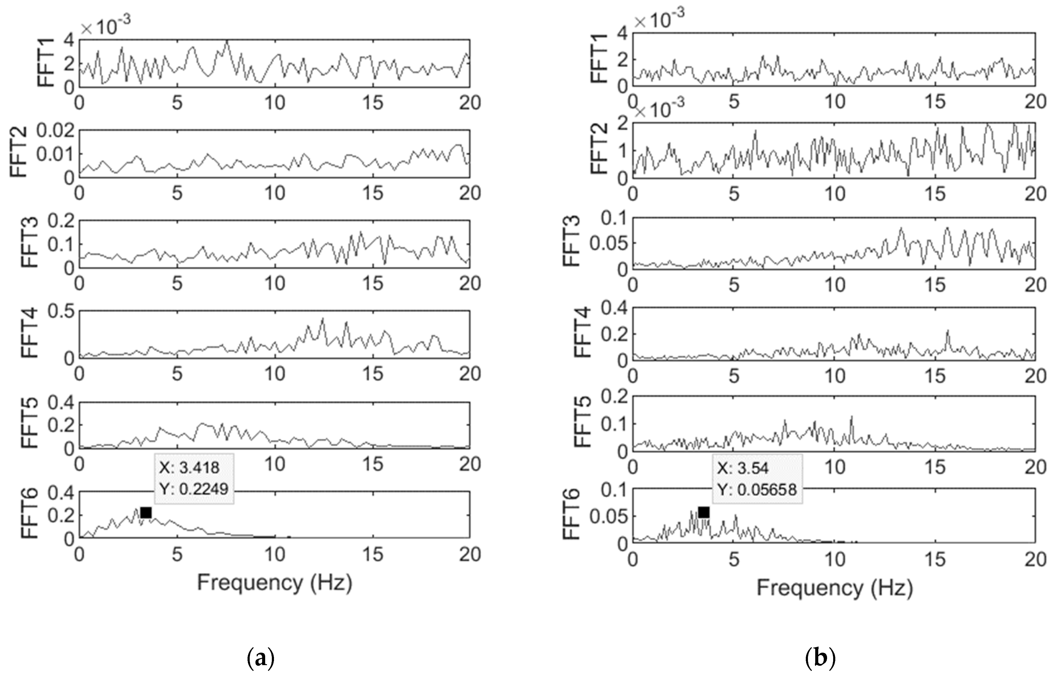
4.2. Effect of Noise
4.3. Effect of Vehicle Velocity
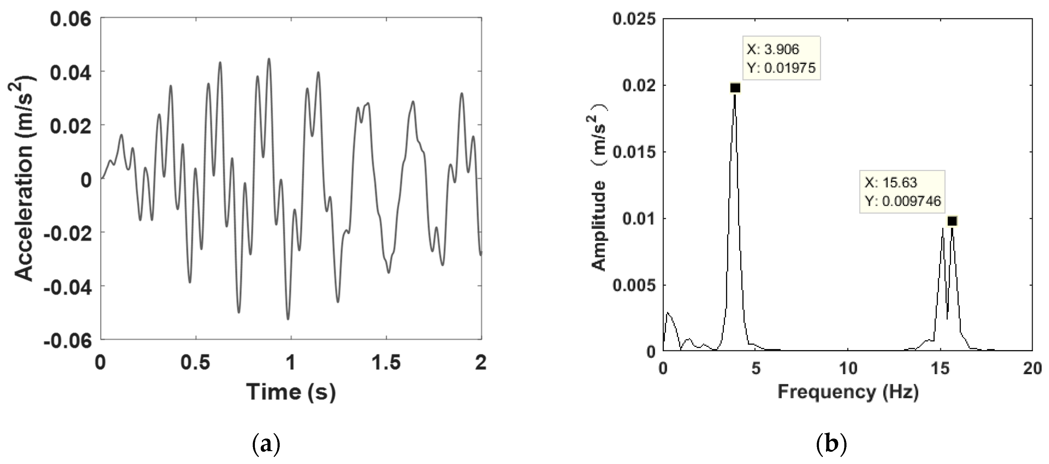
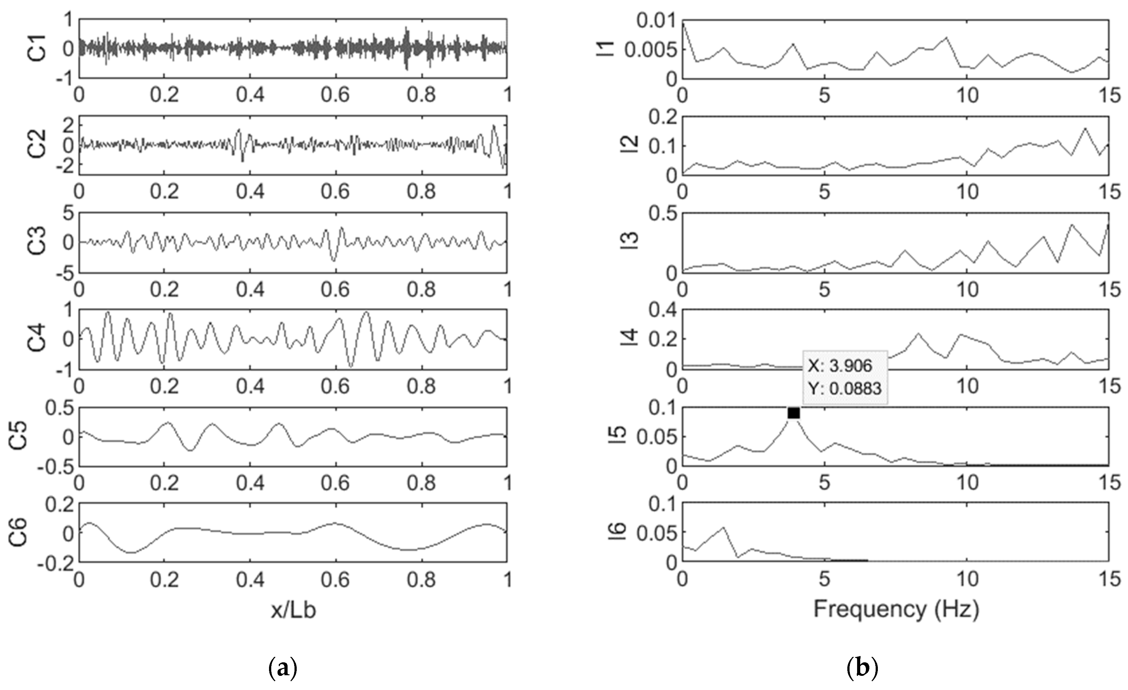
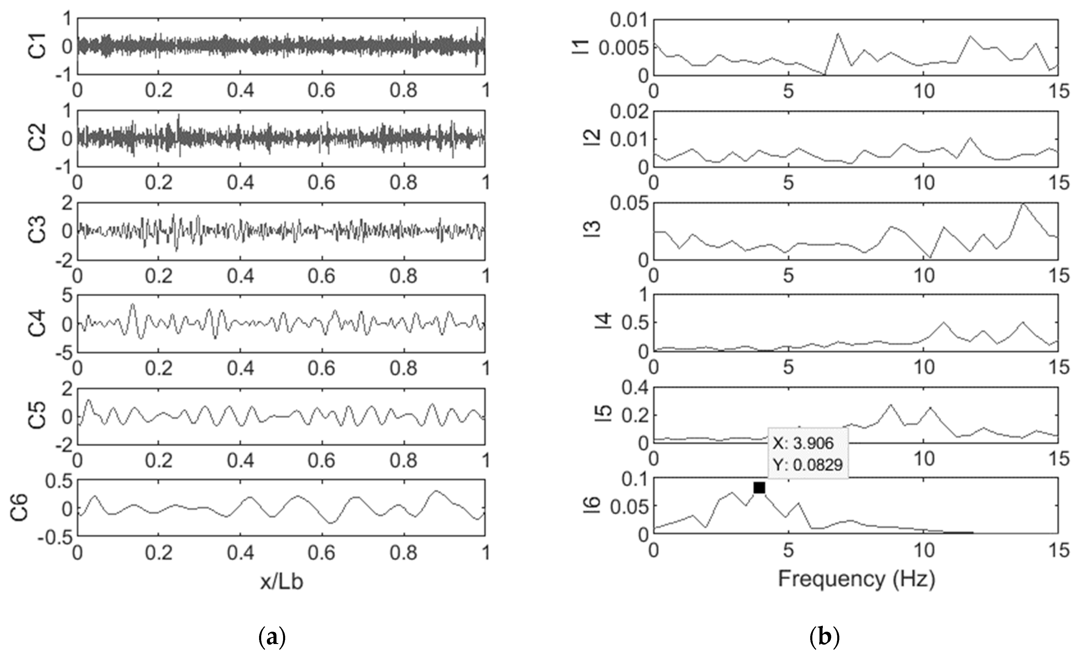
5. Estimation of Vehicle Frequency Using the EEMD Method
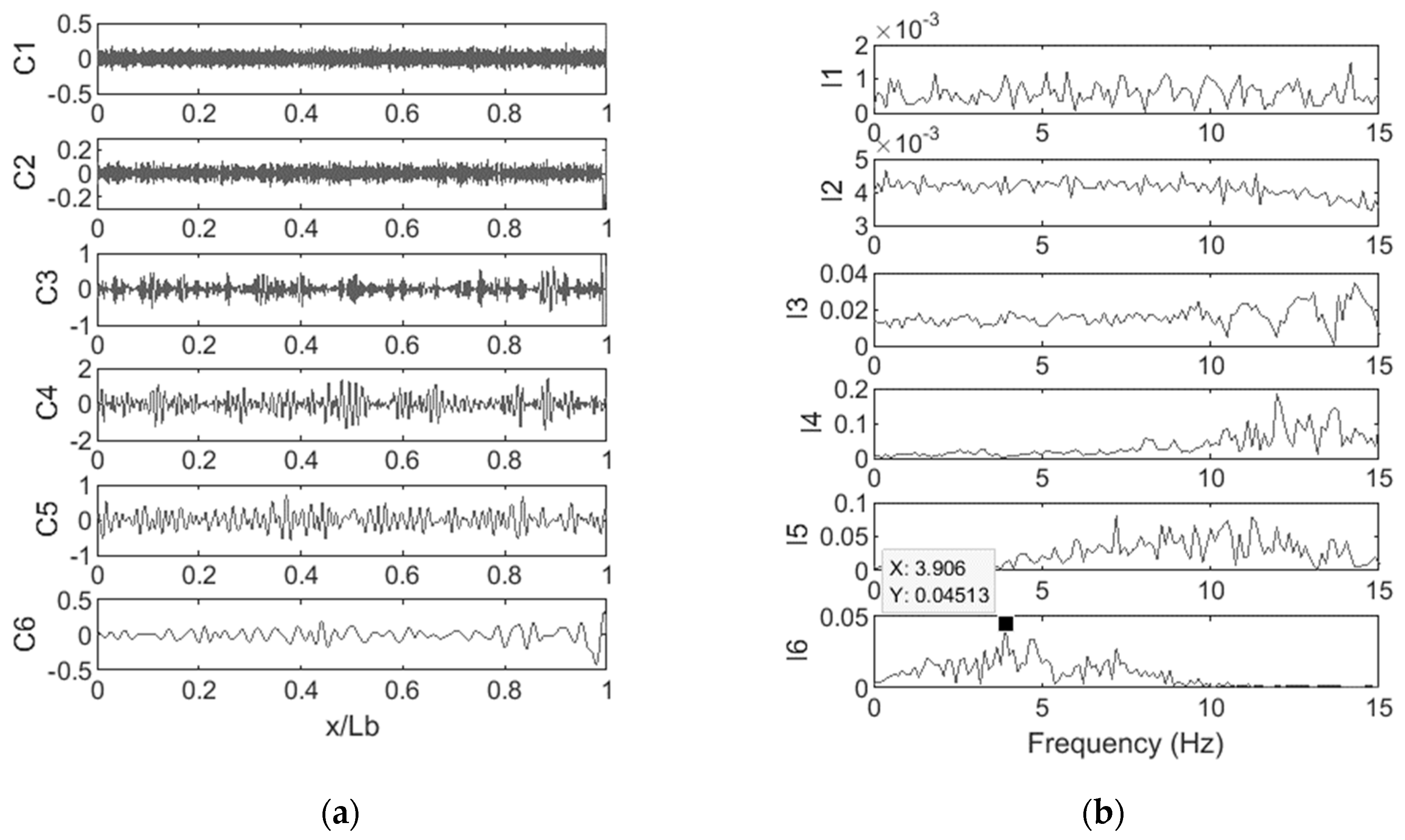
5.1. Effect of Measurement Noise
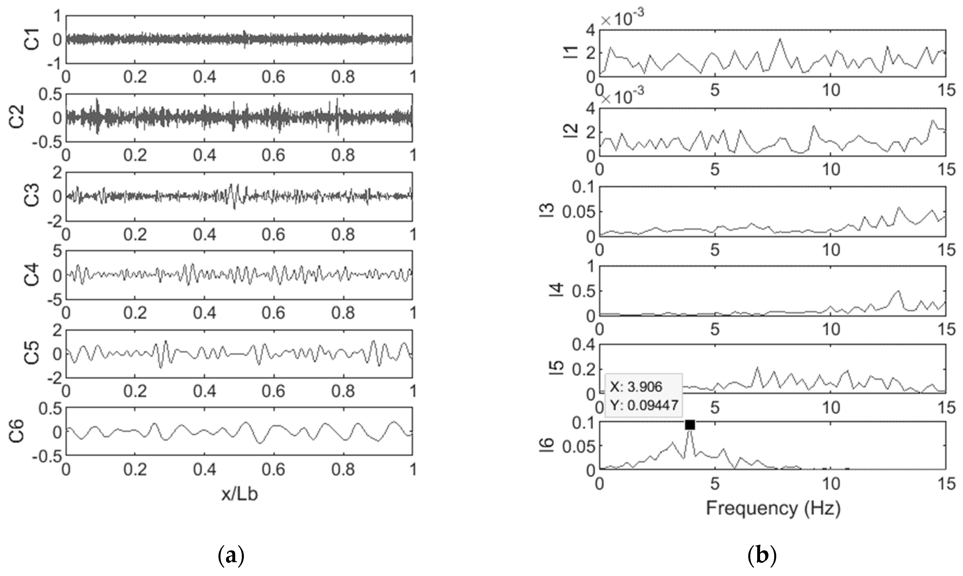
5.2. Effect of Vehicle Velocity
6. Conclusions
Author Contributions
Funding
Conflicts of Interest
References
- Carden, E.P.; Fanning, P. Vibration based condition monitoring: A review. Struct. Health Monit. 2004, 3, 355–377. [Google Scholar] [CrossRef]
- Yang, Y.B.; Lin, C.W.; Yau, J.D. Extracting bridge frequencies from the dynamic response of a passing vehicle. J. Sound Vib. 2004, 272, 471–493. [Google Scholar] [CrossRef]
- Malekjafarian, A.; McGetrick, P.J.; OBrien, E.J. A Review of Indirect Bridge Monitoring Using Passing Vehicles. Shock Vib. 2015, 2015. [Google Scholar] [CrossRef]
- Yang, Y.B.; Yang, J.P. State-of-the-Art Review on Modal Identification and Damage Detection of Bridges by Moving Test Vehicles. Int. J. Struct. Stab. Dyn. 2018, 18, 1850025. [Google Scholar] [CrossRef]
- Bu, J.Q.; Law, S.S.; Zhu, X.Q. Innovative bridge condition assessment from dynamic response of a passing vehicle. J. Eng. Mech. 2006, 132, 1372–1379. [Google Scholar] [CrossRef]
- Oshima, Y.; Yamaguchi, T.; Kobayashi, Y.; Sugiura, K. Eigenfrequency estimation for bridges using the response of a passing vehicle with excitation system. In Proceedings of the Fourth International Conference on Bridge Maintenance, Safety and Management, Seoul, Korea, 13–17 July 2008; pp. 3030–3037. [Google Scholar]
- Yang, Y.B.; Chang, K.C. Extracting the bridge frequencies indirectly from a passing vehicle: Parametric study. Eng. Struct. 2009, 31, 2448–2459. [Google Scholar] [CrossRef]
- Gonzalez, A.; OBrien, E.J.; McGetrick, P.J. Identification of damping in a bridge using a moving instrumented vehicle. J. Sound Vib. 2012, 331, 4115–4131. [Google Scholar] [CrossRef] [Green Version]
- Malekjafarian, A.; Brien, E.J. Identification of bridge mode shapes using Short Time Frequency Domain Decomposition of the responses measured in a passing vehicle. Eng. Struct. 2014, 81, 386–397. [Google Scholar] [CrossRef] [Green Version]
- Malekjafarian, A.; OBrien, E.J. On the use of a passing vehicle for the estimation of bridge mode shapes. J. Sound Vib. 2017, 397, 77–91. [Google Scholar] [CrossRef] [Green Version]
- Yang, J.P.; Lee, W.C. Damping Effect of a Passing Vehicle for Indirectly Measuring Bridge Frequencies by EMD Technique. Int. J. Struct. Stab. Dyn. 2018, 18, 1850008. [Google Scholar] [CrossRef]
- OBrien, E.J.; Malekjafarian, A.; Gonzalez, A. Application of empirical mode decomposition to drive-by bridge damage detection. Eur. J. Mech. A-Solids 2017, 61, 151–163. [Google Scholar] [CrossRef]
- Dhakal, S.; Malla, R.B. Determination of Natural Frequencies of a Steel Railroad Bridge Using Onboard Sensors. In Proceedings of the 16th Biennial ASCE Aerospace Division International Conference on Engineering, Science, Construction, and Operations in Challenging Environments, Cleveland, OH, USA, 9–12 April 2018; pp. 1034–1046. [Google Scholar]
- Kong, X.; Cai, C.S.; Deng, L.; Zhang, W. Using Dynamic Responses of Moving Vehicles to Extract Bridge Modal Properties of a Field Bridge. J. Bridge Eng. 2017, 22, 04017018. [Google Scholar] [CrossRef]
- Mei, Q.; Gül, M.; Boay, M. Indirect health monitoring of bridges using Mel-frequency cepstral coefficients and principal component analysis. Mech. Syst. Signal Process. 2019, 119, 523–546. [Google Scholar] [CrossRef]
- Mei, Q.; Gül, M. A crowdsourcing-based methodology using smartphones for bridge health monitoring. Struct. Health Monit. 2018. [Google Scholar] [CrossRef]
- Aied, H.; Gonzalez, A.; Cantero, D. Identification of sudden stiffness changes in the acceleration response of a bridge to moving loads using ensemble empirical mode decomposition. Mech. Syst. Signal Process. 2016, 66, 314–338. [Google Scholar] [CrossRef]
- Huang, N.E.; Shen, Z.; Long, S.R.; Wu, M.L.C.; Shih, H.H.; Zheng, Q.N.; Yen, N.C.; Tung, C.C.; Liu, H.H. The empirical mode decomposition and the Hilbert spectrum for nonlinear and non-stationary time series analysis. Proc. R. Soc. Lond. Ser. A Math. Phys. Eng. Sci. 1998, 454, 903–995. [Google Scholar] [CrossRef]
- Wu, Z.; Huang, N.E. Ensemble empirical mode decomposition: A noise-assisted data analysis method. Adv. Adapt. Data Anal. 2009, 1, 1–41. [Google Scholar] [CrossRef]
- International Standard Organization. Mechanical Vibration-Road Surface Profiles-Reporting of Measured Data; ISO8608:1995; International Organization for Standardization: Geneva, Switzerland, 1995. [Google Scholar]
- Tedesco, J.W.; McDougal, W.G.; Ross, C.A. Structural dynamics: Theory and Applications; Longman; Addison Wesley: Boston, MA, USA, 1999. [Google Scholar]


| Extracted Frequency in Presence of 5% Noise (Hz) | Error Compared to the FE Frequency (%) | ||
|---|---|---|---|
| EMD method | 3.418 Hz | 10.73% | |
| EEMD method | 3.906 Hz | 2.01% | |
| Speed = 5 m/s | Speed = 10 m/s | ||||
|---|---|---|---|---|---|
| Frequency (Hz) | Error to FE (%) | Frequency (Hz) | Error to FE (%) | ||
| EMD method | 3.54 Hz | 7.55% | 3.41 Hz | 10.73% | |
| EEMD method | 3.90 Hz | 2.01% | 3.90 Hz | 2.01% | |
© 2019 by the authors. Licensee MDPI, Basel, Switzerland. This article is an open access article distributed under the terms and conditions of the Creative Commons Attribution (CC BY) license (http://creativecommons.org/licenses/by/4.0/).
Share and Cite
Zhu, L.; Malekjafarian, A. On the Use of Ensemble Empirical Mode Decomposition for the Identification of Bridge Frequency from the Responses Measured in a Passing Vehicle. Infrastructures 2019, 4, 32. https://0-doi-org.brum.beds.ac.uk/10.3390/infrastructures4020032
Zhu L, Malekjafarian A. On the Use of Ensemble Empirical Mode Decomposition for the Identification of Bridge Frequency from the Responses Measured in a Passing Vehicle. Infrastructures. 2019; 4(2):32. https://0-doi-org.brum.beds.ac.uk/10.3390/infrastructures4020032
Chicago/Turabian StyleZhu, Licheng, and Abdollah Malekjafarian. 2019. "On the Use of Ensemble Empirical Mode Decomposition for the Identification of Bridge Frequency from the Responses Measured in a Passing Vehicle" Infrastructures 4, no. 2: 32. https://0-doi-org.brum.beds.ac.uk/10.3390/infrastructures4020032