Automated Three-Dimensional Linear Elements Extraction from Mobile LiDAR Point Clouds in Railway Environments


1
Faculdade de Ciências, Universidade de Lisboa, 1749-016 Lisboa, Portugal
2
LandCOBA, Digital Cartography Consulting Lda, Av. 5 de Outubro, 323, 1649-011 Lisboa, Portugal
3
Instituto Dom Luiz, Universidade de Lisboa, 1749-016 Lisboa, Portugal
*
Author to whom correspondence should be addressed.
Infrastructures 2019, 4(3), 46; https://0-doi-org.brum.beds.ac.uk/10.3390/infrastructures4030046
Submission received: 27 June 2019
/
Revised: 24 July 2019
/
Accepted: 26 July 2019
/
Published: 30 July 2019
Abstract
:The railway structures need constant monitoring and maintenance to ensure the train circulation safety. Quality information concerning the infrastructure geometry, namely the three-dimensional linear elements, are crucial for that processes. Along with this work, a method to automated extract three-dimensional linear elements from point clouds collected by terrestrial mobile LiDAR systems along railways is presented. The proposed method takes advantage of the stored cloud point’s attributes as an alternative to complex geometric methods applied over the point’s cloud coordinates. Based on the assumption that the linear elements to extract are roughly parallel to the rail tracks and therefore to the system trajectory, the stored scan angle value was used to restrict the number of cloud points that represents the linear elements. A simple algorithm is then applied to that restricted number of points to get the three-dimensional polylines geometry. The obtained values of completeness, correctness and quality, validate the use of the methodology for linear elements extraction from mobile LiDAR data gathered along railway environments.
Keywords:
railway; mobile LiDAR; point cloud; object recognition; railway tracks; ballast; break-line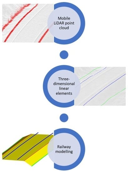
1. Introduction
The railway infrastructure monitoring and surrounding environment maintenance are essential to ensure the train circulation safety. Preventive interventions are crucial, namely due to the gauge monitoring, ballast assessment and surrounding slopes maintenance. In order to define that interventions, it is necessary to have a good knowledge of the railway geometry and surrounding environments. Three-dimensional modelling of the railway’s surrounding environment is a constant need in order to restore safety levels due to the inevitable wear and tear of the railroad over the time. Given the large railroad network extension and access limitation, this can be highly demanding and expensive. Based on the symmetry of the standard railway construction profile, a rough parallel set of linear elements surrounds the rail track, and namely the ballast limits, electrical lines, break-lines, etc., can be determined. The three-dimensional representation of those linear elements is fundamental to the railroad and surrounding environment modelling.
The use of traditional methods to collect that information, namely the total stations and Global Navigation Satellite System (GNSS) surveying, is a very demanding task. Apart from time spent, these methods usually require safety measures for the operations, which imply disruptions or even interruption of the railway operation.
Terrestrial Mobile LiDAR Systems (MLS) installed on moving vehicles have emerged in recent years as a new source of very detailed georeferenced information. Mounted on trains, they eliminate the need for pedestrian access to the railway, while gathering dense and precise information of the railway surrounding area. There are essentially two MLS installation solutions to collect the point clouds along the railway: mounted directly on the train or mounted on a car transported by the train. Despite the different advantages and disadvantages of those different solutions, there are no significant accuracy differences in the obtained cloud points [1].
However, the MLS gathered point clouds are non-selective, i.e., they represent all of the elements in the sensor surrounding at a given moment, without any sort of classification. This makes it impossible to distinguish between points that represent the ground, vegetation, poles, rail tracks, persons or any other object within the sensor range. It is then the necessary method’s implementation that allows an efficient classification of the points that represents a specific object among the millions of the cloud points.
In last few years, the use of LiDAR data has progressively increased, and several studies have been published where this type of data are used for railway infrastructures monitoring, such as tunnels [2,3], railway gauge [1], railway bridges [4], rail surface monitoring and quality indexing [5] and rail surface defect detection [6].
Some studies have focused on extracting point elements from MLS data, like catenary systems [7], poles [8], trees [9] and traffic signals [10]. In [11], previous existing algorithms are adapted to extract several nonlinear objects from the railway environments, namely buildings [12], electric poles and vertical signals [13], trees [14] and ground points [15].
Regarding linear elements extraction, the automatic extraction of railway tracks lines is clearly the most recurrent subject in the existing bibliography about the use of MLS point clouds in railway environments [16]. In [17], the signal intensity reflectance is used to isolate the cloud points that represent the rail tracks from the remaining data, and then the geometric characteristics of the rail tracks are used for modelling and extraction. The study presented in [18] takes advantage of the MLS point clouds decomposition in accurate profiles. By preforming the matching between each system gathered profile and creating a template profile of the infrastructure elements, the rail tracks and turnouts are detected. In [19], the method uses an integrated data-driven and model-driven approach, enhanced by fitting a 2D grid to track bed and by employing template matching to eliminate rail track false positives. The algorithm presented in [20] makes the classification of a small part of the cloud points (based on height), allowing the application for a railway with small slopes, which then uses the Eigen decomposition to select the cloud points representing the rail tracks, ensuring the method operationality regardless their size. The work presented in [21] proposes a Conditional Random Field classifier developed based, which would be the MLS point clouds converted into a set of line segments to which the labelling process is applied. Support Vector Machine (SVM) is then used as a local classifier, which considers only the node features for producing the unary potentials of the CRF mode as a way to classify the different railway electrification system objects using MLS data.
In [22], a fast algorithm to extract rail using MLS data is presented. The method requires data pre-processing to sort the points on each scan line according the signal transmission time, and then the rail tracks are extracted from each scan line based on their shape and relative position. In [23,24], the rail tracks are determined and modelled based on the rail track shape. In the first case, it matches the shape of the ideal rail head with respect to the point cloud by the iterative closest point algorithm. In the second case, it first fits a parametric model of a rail piece to the points along each track, and then estimates the position and orientation parameters of each piece model.
Other linear elements extraction, besides the rail tracks, have been subject of studies but in smaller number. Taking advantage of the fact that a pair of rail tracks is parallel and locally linear, a method to the railroad centreline (axis) determination is presented in [25]. Two approaches are tested; the first determines the centre position directly between points of a pair of rails. The second approach makes the rail track modelling by fitting a parametric model to the extracted rail points.
In [26], power lines are extracted, taking advantage of its parallelism with the rail tracks and using a self-adaptive space region growing method. Using ALS data, the study presented in [27] uses a four-step method to extract the power lines on urban areas.
The need of a proper ballast section maintenance is highlighted in [28]. The study uses a LiDAR system to get the ballast cross-section, given its importance to railroads from both a safety and ongoing maintenance point of view. The ballast top and bottom terrain break-lines are two crucial linear elements to cross-section creation and railway environment modelling, being that its extraction evaluation is included in this work.
More recently the demand of vector linear elements extraction has increased due the emerging Building Information Modelling (BIM) technology. BIM is a collaborative methodology based on parametric three-dimensional models, centralising different types of geometric and geospatial information. This technology has aroused the interest of more and more researchers, since its application along the railway is the object of several studies [29,30]. The three-dimensional linear elements are a crucial need for railway modelling and for the successful implementation of the BIM model.
In the present work, an efficient generic methodology for the extraction of three-dimensional linear elements along railway environments using point clouds collected by MLS is presented.
The proposed methodology takes advantage of the MLS working principles knowledge, rather than only using the three-dimensional point coordinates and then applying methods to the cloud as a mass of points. Also, it assumes that the linear elements to be extracted are roughly parallel to the railway tracks and consequently to the sensor system trajectory. The proposed methodology is strictly applicable to the situation where the MLS platform is installed in a train and has no freedom to change is trajectory, which happens in the case of systems that are installed on a car traveling along a road.
The remainder of this paper is structured as follows. In Section 2, a description of the MLS working principles and proposed methodology is presented. The obtained results for a real railway point cloud sample are presented in Section 3, with respective completeness, correctness and quality values. Section 4 has a critical analysis of the obtained results and future work ideas. Finally, the overall conclusions are presented.
2. Materials and Methods
2.1. MLS Working Principles and Storing Standard Files Format
Usually, the data registered by the MLS are classified in two types: trajectory data and laser sensor data. The trajectory data include all data that allow the system to compute the most accurate position of the laser sensor along the trajectory.
The laser sensor data consist of a set of distances and angles that allow the ability to compute the point’s coordinates in space in regard to the sensor position. Most commercial systems use a “time of travel” strategy, i.e., the laser sensor emits an electric pulse and the travel time between the emission and the reception moments after being reflected on the object is accurately registered on the sensor.
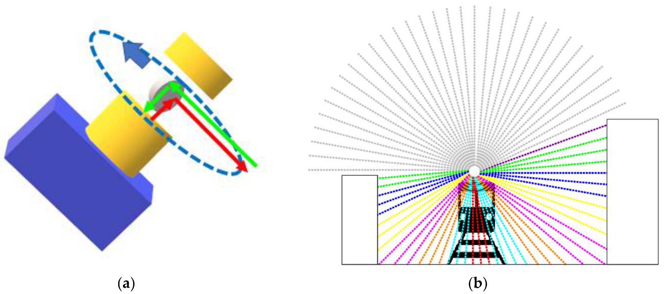
To get the cloud effect and to ensure a full surrounding coverage, two types of movement are applied to the pulse direction. The first is a rotational movement 360° around the sensor axis, creating a cross-section. The second movement results from the vehicle movement in which the sensor is installed, generating the cloud effect through consecutive cross-sections. In Figure 1a, schemas of these two movements are presented.
The LAS file format is a public standard file format for point cloud interchange, which is created and maintained by the American Society for Photogrammetry and Remote Sensing (ASPRS). This binary file format, or a generic ASCII file interchange format used by many companies, is an alternative to proprietary formats. The LAS is a binary file that maintains specific information regarding the LiDAR nature of the data while not being overly complex [31].
The LAS file contains the information regarding each gathered light pulse, including its attributes, namely, its three-dimensional coordinates, GPS epoch, intensity value, scan angle, scan direction, etc. In the 1.4 LAS version [32], the scan angle is defined as the rotational position of the emitted laser pulse with respect to the vertical of the coordinate system of the data. The 2 bytes variable allows the increment of 0.006° interval, positively incremented in the clockwise counter direction from the sensor rear viewpoint, allowing for a value of 30,000 in vertical direction.
Since the publication of LAS version 1.4 is quite recent, there is still no adaptation of most of the processing software for the creation of the LAS files in this version, so throughout this work all used point clouds are stored in LAS version 1.2 file format. Therefore, the scan angle attribute is a 1-byte integer, which only allows for the storage of 255 distinct values. However, it is possible to convert the 360 possible values to the 255 available values in a simple form represented in Equation (1):
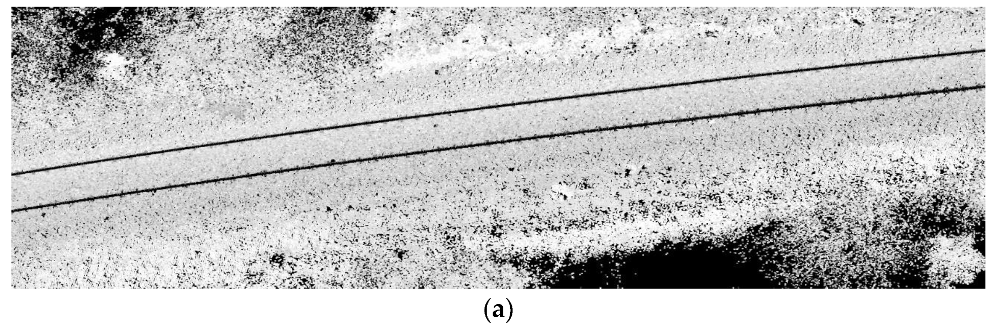
where V255 is the value converted to 1-byte range and V360 is the value of the angle rounded to the degree. Figure 2 represents an extraction from a point cloud obtained by MLS along a railway line and coloured by intensity and scan angle.
V255 = V360 × 255/360
In Figure 2b, it is possible to observe the symmetrical effect of the scan angle values regarding the sensor trajectory. Despite the 255-values conversion limitation, there is still a significant segmentation of the cloud. Figure 3 shows a typical cross-section of the scan angle coloured point cloud.
2.2. Proposed Methodology
The proposed methodology uses the scan angle value to restrict the cloud to a small number of points with the same scan angle value, which represents the linear element to extract. It is assumed, that the linear elements are roughly parallel to MLS trajectory and, consequently, all cloud points that represent them will have approximately the same scan angle. Then, using the restricted classified cloud points, a simple algorithm will be applied to create the three-dimensional linear elements vertices.
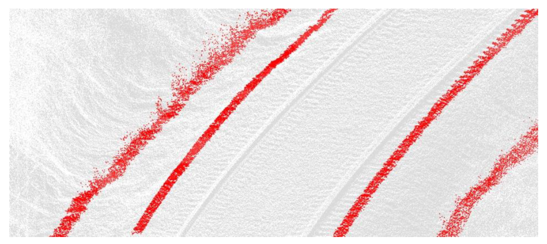
For instance, considering a 0 degrees scan angle, a ground points strip under the sensor trajectory, can be obtained, since the scan angle origin is in sensor nadir direction. In Figure 4, all points with 0 scan angle value are represented in red, and the remaining cloud points are white. It is important to emphasise that throughout this work, all the angle values do not represent the system real measured scan angles, but rather the original value rounded to the nearest integer and converted to the 255-values scale stored in the LAS file.
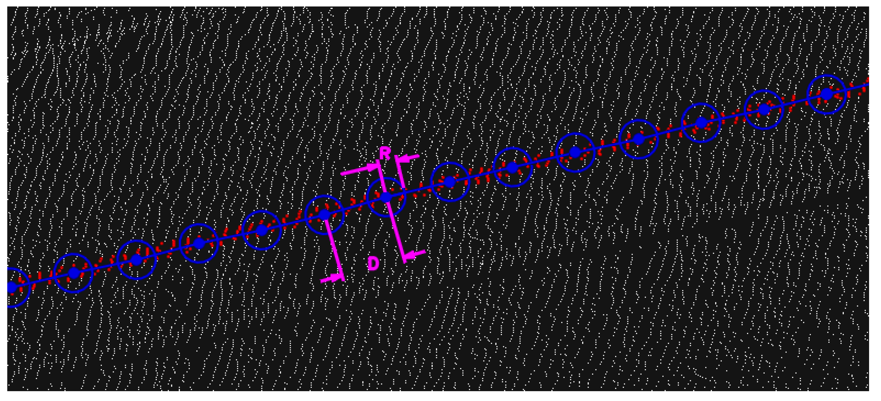
The 0 scan angle values are usually represented the narrower strip points since they are closest to the sensor and have a vertical incidence angle. After the scan angle point classification, it is still necessary to convert the classified cloud points to a vector linear three-dimensional element. To create that element, a value D is defined as the distance between the line vertices. Then for each vertex, the cloud points coordinate average (0 scan angle value) under the distance range (R) are used to compute each vertex position. This simple process works well since the scan angle classified points are always represented by a point strip. Therefore, if R is greater than the strip width, then the coordinate average points will tend to be located along the strip axis. The algorithm illustration schema is presented in Figure 5.
The algorithm starts with the D and R values definition, where D must always be equal or higher than R double. The D value can be adjusted based on the pretended detail for the extracted line. Smaller distance between vertices means greater detail of the extracted line. In the trajectory line example of Figure 5, the coordinate Z results from the average Z coordinates of the classified points. However, depending of the linear element type, the maximum or minimum Z value can be used. A higher R value increases the number of classified points used, which can lead to higher standard deviations and degradation of the Z coordinate accuracy. The R value should be kept near the double of the classified point’s strip width value. For proper method operation, the classified points should be ordered according the trajectory direction. That should happen by default, since it is the acquisition order, otherwise, the GPS epoch attribute can be used to perform that ordering.
The respective method pseudocode is presented below:
- Input: Restricted scan angle classified cloud points
- For each point P
- ○
- If Distance2D (P, Pprev) < D then go to Jump:
- ○
- For each point P1
- ▪
- If Distance2D (P, P1) < R then
- ▪
- PointsList add P1
- ▪
- End if
- ○
- Next
- ○
- Vertex = Average (PointList (X, Y, Z))
- ○
- VertexList add Vertice
- ○
- Clear PointList
- ○
- Jump
- ○
- Set Pprev = P
- Next
- Polyline = Vertexlist
2.3. Rail Tracks Centre Lines
The proposed method for the rail tracks lines extraction is very similar to previously presented to trajectory line extraction.
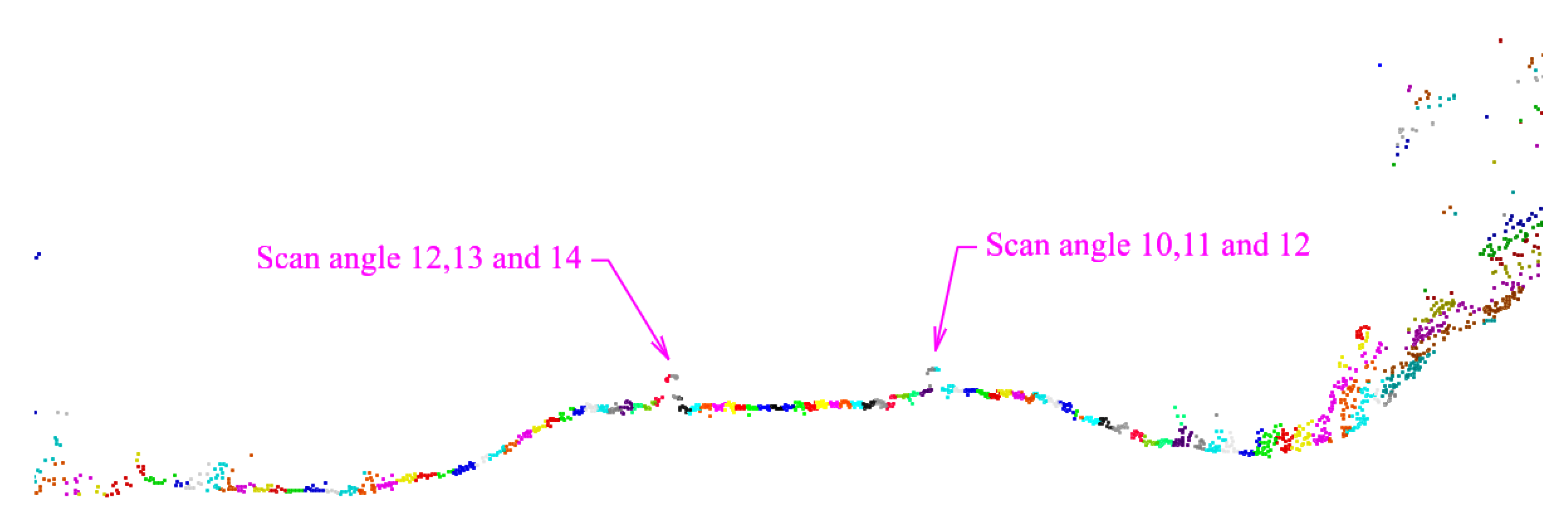
Given the thickness and configuration of the rail tracks, the respective cloud points may have more than one scan angle value, and it is necessary to use several scan angles. In the cross-section example shown in Figure 7, three scan angle values are used for each rail track. The left and right values of the present example are not symmetric since the position of the sensor does not match the railroad axis.
After identifying the scan angles representing each rail track, the element points can be aggregated, as shown in Figure 8.
After the rail track point cloud classification, the centre line creation methodology is very similar to the method described for the trajectory line. As shown in Figure 5, after R and D values are defined, the algorithm is applied. However, instead of using the point’s three-dimensional coordinates average to create the line vertices, just the planimetric average coordinates (X, Y) are used. For the line vertices Z-coordinate, the maximum value of the points at R distance is used.
The use of the point’s maximum Z-coordinate becomes necessary since the resulting line vertices are assumed to have the rail track top altimetric values. This would not happen if the average Z-coordinate of the selected points had been used, since the classified points, due to the R-ray distance, were selected from the top and bottom of the rail. Figure 9 shows an example of the obtained rail tracks top centre lines.
2.4. Ballast Top and Bottom Break-Lines
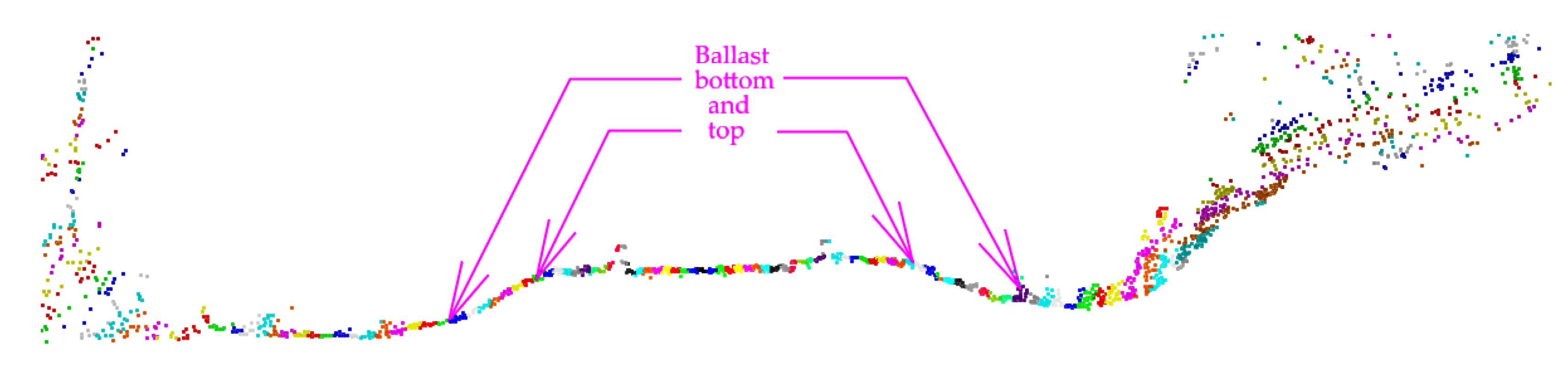
Another example of three-dimensional lines in a railway environment is the terrain break-lines, which play a key role in the digital terrain model quality [34]. A typical case of those lines in railway environments is the ballast top and bottom lines. The ballast maintenance is fundamental to distribute the dynamic loads from the vehicle to the embankment and to ensure the track stability, and the ballast cross-section (profile) it is critical to do that maintenance [28,35,36]. As a way to model the ballast surface and create consecutive ballast cross-sections, it is necessary to design the top and bottom ballast break-lines. In Figure 10, the lateral ballast area, comprehended between the top and bottom break-lines, is indicated.
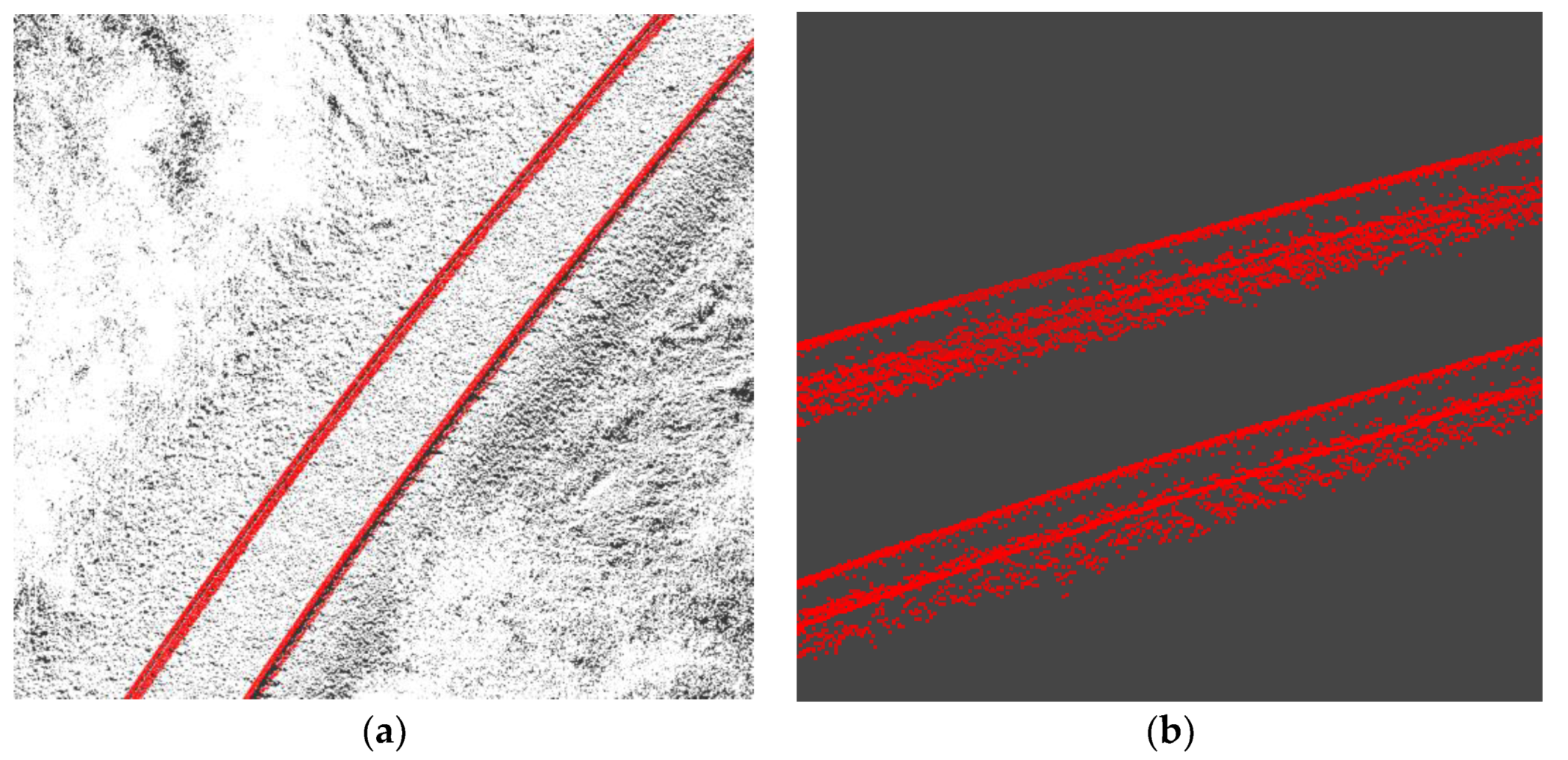
To apply the proposed method to the top and bottom ballast lines extraction, it is necessary to identify the scan angle value of the cloud points that represent it. Once more, consecutive scan angle values can be used to unsure that both lines to extract are included in the classified points. An example of the obtained results, after the classification and aggregation of the angle values, can be seen in Figure 11.
Figure 10 and Figure 11 shows a greater dispersion of the classified points in the ballast bottom. Such point dispersion occurs due to the existence of growing vegetation and grassy areas. Since, if at least one of the points contained in the R distance of Figure 5 reached the ground, then the point with the minimum Z-coordinate will also be on the ground. In way to eliminate the vegetation effect, the minimum Z-coordinate of the points was used for each line vertex. Figure 12 shows the result obtained for the ballast top and bottom lines.
3. Results
In order to test the proposed methodology for the extraction of three-dimensional lines in a railway environment, a point cloud obtained by an SLMT installed in a train was used with the sensor RIEGL VQ-250. The cloud covered area is approximately 550 m long. Table 1 shows the sensor main characteristics.
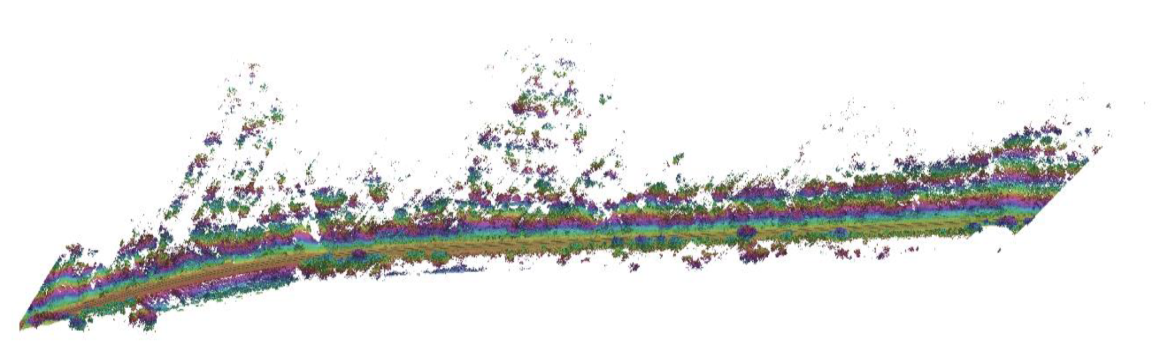
After data acquisition, the trajectory was processed using the IMU and GNSS data and subsequently integrated with the distances and angles collected by the laser sensor. The obtained georeferenced point cloud was exported to LAS format, version 1.2. Figure 13 presents the point cloud coloured by elevation.
Several cross-sections were created along the cloud and materialised in a CAD software to identify the point’s scan angle values that represent the lines to be extracted. The cross-section points were coloured, and each scan angle value was assigned to a colour in the CAD environment, getting results like Figure 3, Figure 7 and Figure 10.
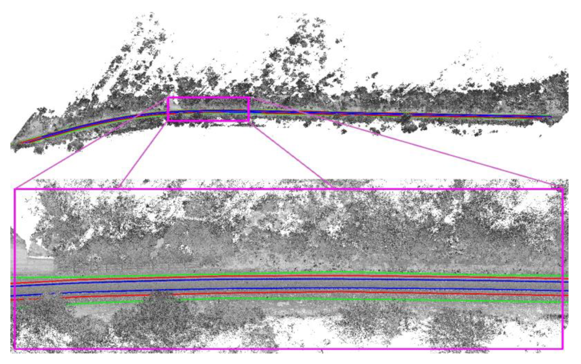
Once the point’s scan angle values were identified, based on the pseudocode presented in Section 2.2, a C# algorithm allows the generation of the extracted three-dimensional lines. Figure 14 highlights three-dimensional lines obtained, and the modelling result is presented in Figure 15.
In Figure 15, the blue lines represent the rail track top (head) middle line, directly extracted from the point cloud. Other railway elements can be obtained, such as the rail track axis line (centre of the two tracks), resulting from the average coordinates of those two lines. The rail gauge, defined as the minimum distance between the two rail tracks, can be calculated from the tracks middle centre line’s minimum distance (less than the track width value). Even the entire track shape can be modelled using its parametric values [25].
To evaluate the quality results, the linear elements have been also manually extracted. The manual process was performed through a consecutive cross-section along the point cloud. In CAD software, all key points of the rails and ballast lines were marked in each cross-section. The manual extracted lines result from the sequential union of those key points.
For each line vertex extracted through the automated proposed methodology, the three-dimensional distance of the manual digitised line was measured. Based on those values, the accuracy metrics of completeness, correctness and quality, usually used on such assessments [17], were calculated for the proposed method evaluation by:
where TP is the true positive length, i.e., the line’s length at less than 5 cm distance in both manual and automated extraction datasets; FN is the false negative length, i.e., the length of the manual lines where the distance to the automated extracted is higher than 5 cm; and FP is the false positive length, i.e., the length of the automated extracted lines where the distance to the manual is higher than 5 cm. Table 2 lists the completeness, correctness, and quality values obtained for the proposed method, when compared with the manual digitalised lines.
4. Discussion
The ballast lines have lower accuracy than the rail tracks centre lines. That happens because those lines are much less defined, and the 5 cm R-ray circle that is used is very tight. By increasing such limit distance to 15 cm, all lines quality measurement accuracy increases up to 85%. It should be noted that the number of manual digitalised line vertices is much lower than the vertices number of the proposed methodology extracted line. The reason is due to the used manual process; the number of cross-sections traced by the operator depends on the perception of the line’s direction and height variation, while in the proposed methodology, the number of vertices depends of the pre-defined D-distance between vertices.
Also, mainly due to the terrain slope variation, the ballast width will change and consequently the cloud points scan angle, representing the top and bottom ballast break-lines, will also change. In larger datasets, it may be necessary to have additional restrictions to the scan angle classified points. In future work, the decomposition of the scan angle classified cloud points in the original scan profiles, and the application of height and slope thresholds values to the individual profile points, should be tested and analysed to obtain the best perform. Such restrictions, in addition to the scan angle classified cloud points, may well be a solution to overcome that issue.
Although not fully automatic, the method implementation is very simple, and the execution is very fast, extracting all lines along the 550 m of the used dataset in less than 1 min.
The detail level definition of the extracted lines, through the threshold values definition (R and D of Figure 5), is another advantage of the proposed method.
Regardless of being a standard format, the performed tests showed that many of the MLS data processing software do not yet use the correct LAS specifications. For example, the Optech LAS files generated by the LMS Pro version processing software have a continuous value from 0 to 255, increasing anticlockwise. While, in the software Trimble Trident version 7.1, the LAS Files has a zero value for the scan angle for all cloud points.
In future works, the use of the 1.4 version LAS files, which have a much higher definition of the scan angle, should allow for a higher versatility and a greater accuracy.
5. Conclusions
Throughout this work, a different approach for three-dimensional linear elements extraction from mobile LiDAR point clouds in railway environments is presented. This takes advantage of the linear elements that are being extracted, which are roughly parallel to the railway tracks and consequently to the sensor system trajectory. The proposed methodology uses the scan angle variable to restrict the number of cloud points, and the method simplifies the linear elements extraction.
Beyond the obtained results, this work intends to highlight the potential of the stored information for each point in an LAS file and for the classification and extraction process of point cloud elements.
Author Contributions
Conceptualisation, L.G.; Formal analysis, L.G. and C.A.; Investigation, L.G.; Methodology, L.G.; Supervision, C.A.; Writing—Original draft, L.G.; Writing—Review & editing, L.G. and C.A.
Funding
This research received no external funding.
Conflicts of Interest
The authors declare no conflict of interest.
References
- Mikrut, S.; Kohut, P.; Pyka, K.; Tokarczyk, R.; Barszcz, T.; Uhl, T. Mobile laser scanning systems for measuring the clearance gauge of railways: State of play, testing and outlook. Sensors 2016, 16, 683. [Google Scholar] [CrossRef] [PubMed]
- Han, J.; Guo, J.; Chiang, Y. Monitoring tunnel profile by means of multi-epoch dispersed 3-D LiDAR point clouds. Tunn. Undergr. Space Technol. 2013, 33, 186–192. [Google Scholar] [CrossRef]
- Xie, X.; Lu, X. Development of a 3D Modelling Algorithm for Tunnel Deformation Monitoring Based on Terrestrial Laser Scanning. Undergr. Space 2107, 2, 16–29. [Google Scholar] [CrossRef]
- Gawronek, P.; Makuch, M. TLS Measurement during Static Load Testing of a Railway Bridge. ISPRS Int. J. Geo Inf. 2019, 8, 44. [Google Scholar] [CrossRef]
- Taheri Andani, M.; Mohammed, A.; Jain, A.; Ahmadian, M. Application of LIDAR technology for rail surface monitoring and quality indexing. Proc. Inst. Mech. Eng. Part F J. Rail Rapid Transit. 2018, 232, 1398–1406. [Google Scholar] [CrossRef]
- Xiong, Z.; Li, Q.; Mao, Q.; Zou, Q. A 3D Laser Profiling System for Rail Surface Defect Detection. Sensors 2017, 17, 1791. [Google Scholar] [CrossRef]
- Pastucha, E. Catenary System Detection, Localization and Classification Using Mobile Scanning Data. Remote Sens. 2016, 8, 801. [Google Scholar] [CrossRef]
- Rodríguez-Cuenca, B.; García-Cortés, S.; Ordóñez, C.; Alonso, M.C. Automatic detection and classification of pole-like objects in urban point cloud data using an anomaly detection algorithm. Remote Sens. 2015, 7, 12680–12703. [Google Scholar] [CrossRef]
- Yu, Y.; Li, J.; Guan, H.; Zai, D.W. Automated Extraction of 3D Trees from Mobile LiDAR Point Clouds. ISPRS Int. Arch. Photogramm. 2014, 40, 629. [Google Scholar] [CrossRef]
- Gargoum, S.; El-Basyouny, K.; Sabbagh, J.; Froese, K. Automated Highway Sign Extraction Using Lidar Data. Transp. Res. Rec. J. Transp. Res. Board 2017, 2643, 1–8. [Google Scholar] [CrossRef] [Green Version]
- Zhu, L.; Hyyppä, J. The Use of Airborne and Mobile Laser Scanning for Modelling Railway Environments in 3D. Remote Sens. 2014, 6, 3075–3100. [Google Scholar] [CrossRef]
- Zhu, L.; Hyyppa, J.; Kukko, A.; Kaartinen, H.; Chen, R. Photorealistic 3D city modeling from mobile laser scanning data. Remote Sens. 2011, 3, 1406–1426. [Google Scholar] [CrossRef]
- The Use of Mobile Laser Scanning Data and Unmanned Aerial Vehicle Images for 3D Model Reconstruction. Available online: http://www.int-arch-photogramm-remote-sens-spatial-inf-sci.net/XL-1-W2/419/2013/isprsarchives-XL-1-W2-419-2013.pdf (accessed on 21 June 2019).
- Hyyppa, J.; Hyyppa, H.; Leckie, D.; Gougeon, F.; Yu, X.; Maltamo, M. Review of methods of small footprint airborne laser scanning for extracting forest inventory data in boreal forests. Int. J. Remote Sens. 2008, 29, 1339–1366. [Google Scholar] [CrossRef]
- Axelsson, P. DEM generation from laser scanner data using adaptive TIN models. Int. Arch. Photogramm. Remote Sens. 2000, 33, 110–117. [Google Scholar]
- Che, E.; Jung, J.; Olsen, M.J. Object Recognition, Segmentation, and Classification of Mobile Laser Scanning Point Clouds: A State-of-the-Art Review. Sensors 2019, 19, 810. [Google Scholar] [CrossRef] [PubMed]
- Yang, B.; Fang, L. Automated extraction of 3-D railway tracks from mobile laser scanning point clouds. IEEE J. Sel. Top. Appl. Earth Obs. Remote Sens. 2014, 7, 4750–4761. [Google Scholar] [CrossRef]
- Stein, D.; Spindler, M.; Kuper, J.; Lauer, M. Rail detection using lidar sensors. Int. J. Sustain. Dev. Plan. 2016, 11, 65–78. [Google Scholar] [CrossRef] [Green Version]
- Arastounia, M.; Oude Elberink, S. Application of Template Matching for Improving Classification of Urban Railroad Point Clouds. Sensors 2016, 16, 2112. [Google Scholar] [CrossRef]
- Arastounia, M. An Enhanced Algorithm for Concurrent Recognition of Rail Tracks and Power Cables from Terrestrial and Airborne LiDAR Point Clouds. Infrastructures 2017, 2, 8. [Google Scholar] [CrossRef]
- Jung, J.; Chen, L.; Sohn, G.; Luo, C.; Won, J. Multi-Range Conditional Random Field for Classifying Railway Electrification System Objects Using Mobile Laser Scanning Data. Remote Sens. 2016, 8, 1008. [Google Scholar] [CrossRef]
- Lou, Y.; Zhang, T.; Tang, J.; Song, W.; Zhang, Y.; Chen, L. A Fast Algorithm for Rail Extraction Using Mobile Laser Scanning Data. Remote Sens. 2018, 10, 1998. [Google Scholar] [CrossRef]
- Niina, Y.; Honma, R.; Honma, Y.; Kondo, K.; Tsuji, K.; Hiramatsu, T.; Oketani, E. Automatic rail extraction and celarance check with a point cloud captured by mls in a railway. Int. Arch. Photogramm. Remote Sens. Spat. Inf. Sci. 2018, 42, 767–771. [Google Scholar] [CrossRef]
- Oude Elberink, S.; Khoshelham, K.; Arastounia, M.; Diaz Benito, D. Rail Track Detection and Modelling in Mobile Laser Scanner Data. ISPRS Ann. Photogramm. Remote Sens. Spat. Inf. Sci. 2013, II-5/W2, 223–228. [Google Scholar] [Green Version]
- Elberink, S.O.; Khoshelham, K. Automatic Extraction of Railroad Centerlines from Mobile Laser Scanning Data. Remote Sens. 2015, 7, 5565–5583. [Google Scholar] [CrossRef] [Green Version]
- Zhang, S.; Wang, C.; Yang, Z.; Chen, Y.; Li, J. Automatic railway power line extraction using mobile laser scanning data. ISPRS Int. Arch. Photogramm. Remote Sens. Spat. Inf. Sci. 2016, XLI-B5, 615–619. [Google Scholar] [CrossRef]
- Wang, Y.J.; Chen, Q.; Liu, L.; Zheng, D.Y.; Li, C.K.; Lim, K. Supervised Classification of Power Lines from Airborne LiDAR Data in Urban Areas. Remote Sens. 2017, 9, 771. [Google Scholar] [CrossRef]
- Zarembski, A.M.; Grissom, G.T.; Euston, T.L. On the Use of Ballast Inspection Technology for the Management of Track Substructure. Transp. Infrastruct. Geotechnol. 2014, 1, 83–109. [Google Scholar] [CrossRef]
- Bensalah, M.; Elouadi, A.; Mharzi, H. Integrating BIM in railway projects: Review & perspectives for Morocco & Mena. Int. J. Recent Sci. Res. 2018, 9, 23398–23403. [Google Scholar]
- Nuttens, T.; De Breuck, V.; Cattor, R.; Decock, K.; Hemeryk, I. Using Bim models for the design of large rail infrastructure projects: Key factors for a successful implementation. Int. J. Sustain. Dev. Plan. 2018, 13, 73–83. [Google Scholar] [CrossRef]
- LASer (LAS) File Format Exchange Activities. Available online: https://www.asprs.org/divisions-committees/lidar-division/laser-las-file-format-exchange-activities (accessed on 22 June 2019).
- LAS Specification 1.4—R14. Available online: http://www.asprs.org/wp-content/uploads/2019/03/LAS_1_4_r14.pdf (accessed on 22 June 2019).
- Douglas, D.; Peucker, T. Algorithms for the reduction of the number of points required to represent a digitized line or its caricature. Cust. Cartogr. 1973, 10, 112–122. [Google Scholar] [CrossRef]
- Yang, B.; Huang, R.; Dong, Z.; Zang, Y.; Li, J. Two-step adaptive extraction method for ground points and breaklines from lidar point clouds. ISPRS J. Photogramm. Remote Sens. 2016, 119, 373–389. [Google Scholar] [CrossRef]
- Zarembski, A.M.; Grissom, G.T.; Euston, T.L. Use of Ballast Inspection Technology for the Prioritization, Planning and Management of Ballast Delivery and Placement. In Proceedings of the American Railway Engineering Association Annual Conference, Indianapolis, IN, USA, 29 September 2013. [Google Scholar]
- Ciotlaus, M.; Kollo, G. Ballast bed cleaning and recycling—Influence on stability of continuously welded rail track. Procedia Manuf. 2108, 22, 294–300. [Google Scholar] [CrossRef]
Figure 1.
Laser sensor working principles schema: (a) Mirror rotation movement deflecting the emitted (red) and received (green) pulse; (b) Schematic representation of the reflected pulses creating a profile effect, coloured by the scan angle (grey pulses are not reflected to the sensor). The point cloud effect results from the train movement through consecutive cross-sections.

Figure 2.
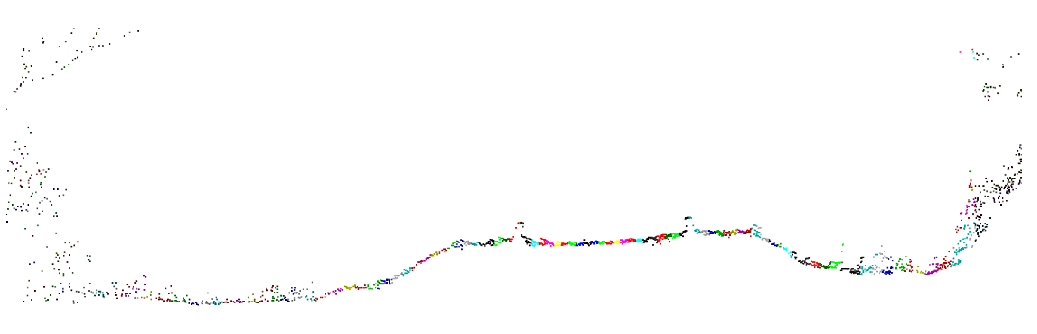
Point cloud sample obtained by an MLS installed in a train along a railway line: (a) Grayscale representation intensity values; (b) Coloured point cloud based on scan angle values converted to 255 values.
Figure 2.
Point cloud sample obtained by an MLS installed in a train along a railway line: (a) Grayscale representation intensity values; (b) Coloured point cloud based on scan angle values converted to 255 values.


Figure 3.
Scan angle coloured point cloud from a cross-section.

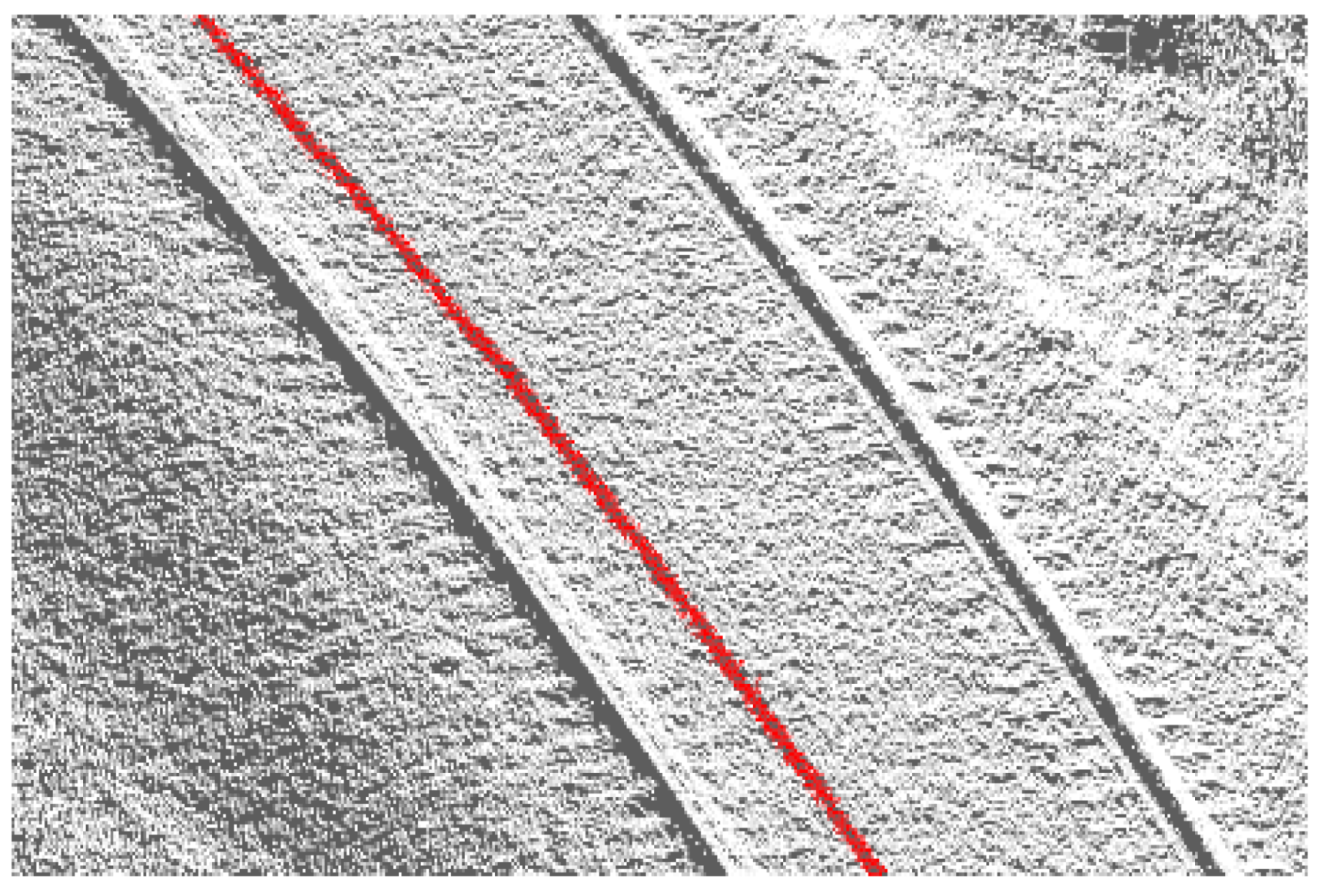
Figure 4.
Point cloud just with the 0 scan angle value points coloured in red.

Figure 5.
Three-dimensional line creation schema based on the classified 0 scan angle value points (red). Each new line vertex coordinates result from the average point coordinates inside each R-ray circle, with D as the approximate distance between vertices.
Figure 5.
Three-dimensional line creation schema based on the classified 0 scan angle value points (red). Each new line vertex coordinates result from the average point coordinates inside each R-ray circle, with D as the approximate distance between vertices.

Figure 6.
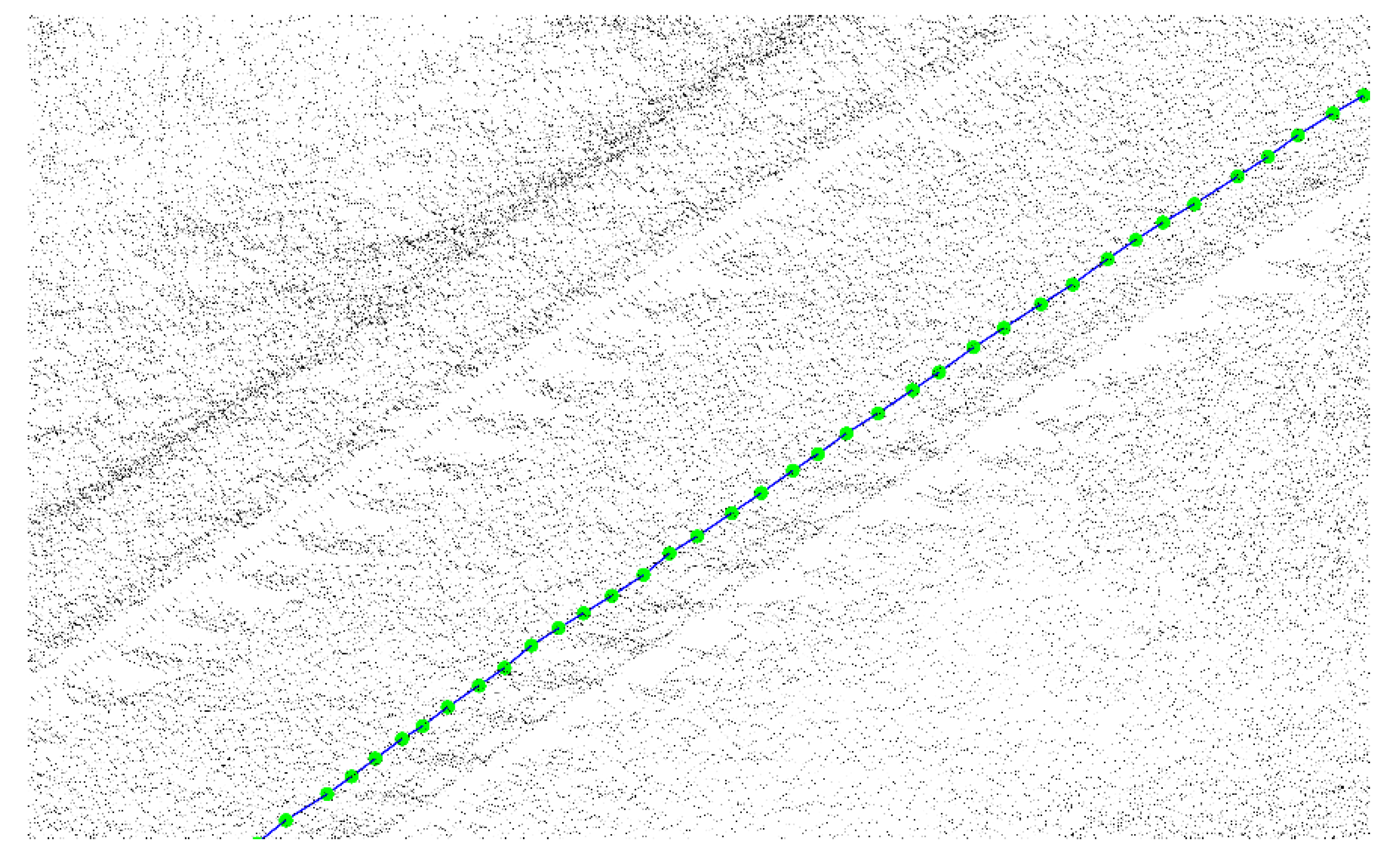
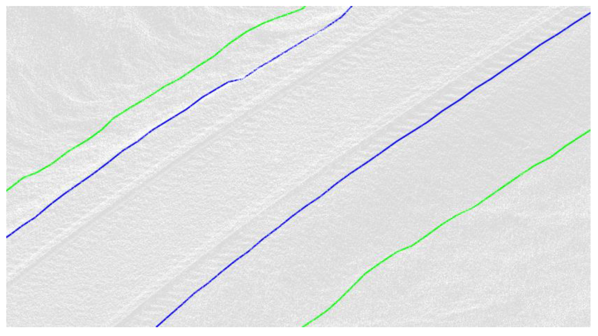
Example of a three-dimensional line extracted, representing the sensor trajectory.

Figure 7.
Scan angle coloured cloud cross-section and scan angle values for rail tracks classification point.
Figure 7.
Scan angle coloured cloud cross-section and scan angle values for rail tracks classification point.

Figure 8.
Rail track point cloud classification: (a) Scan angle classified cloud points, rail track points (red) and remaining points (white); (b) Rail track points detail.
Figure 8.
Rail track point cloud classification: (a) Scan angle classified cloud points, rail track points (red) and remaining points (white); (b) Rail track points detail.

Figure 9.
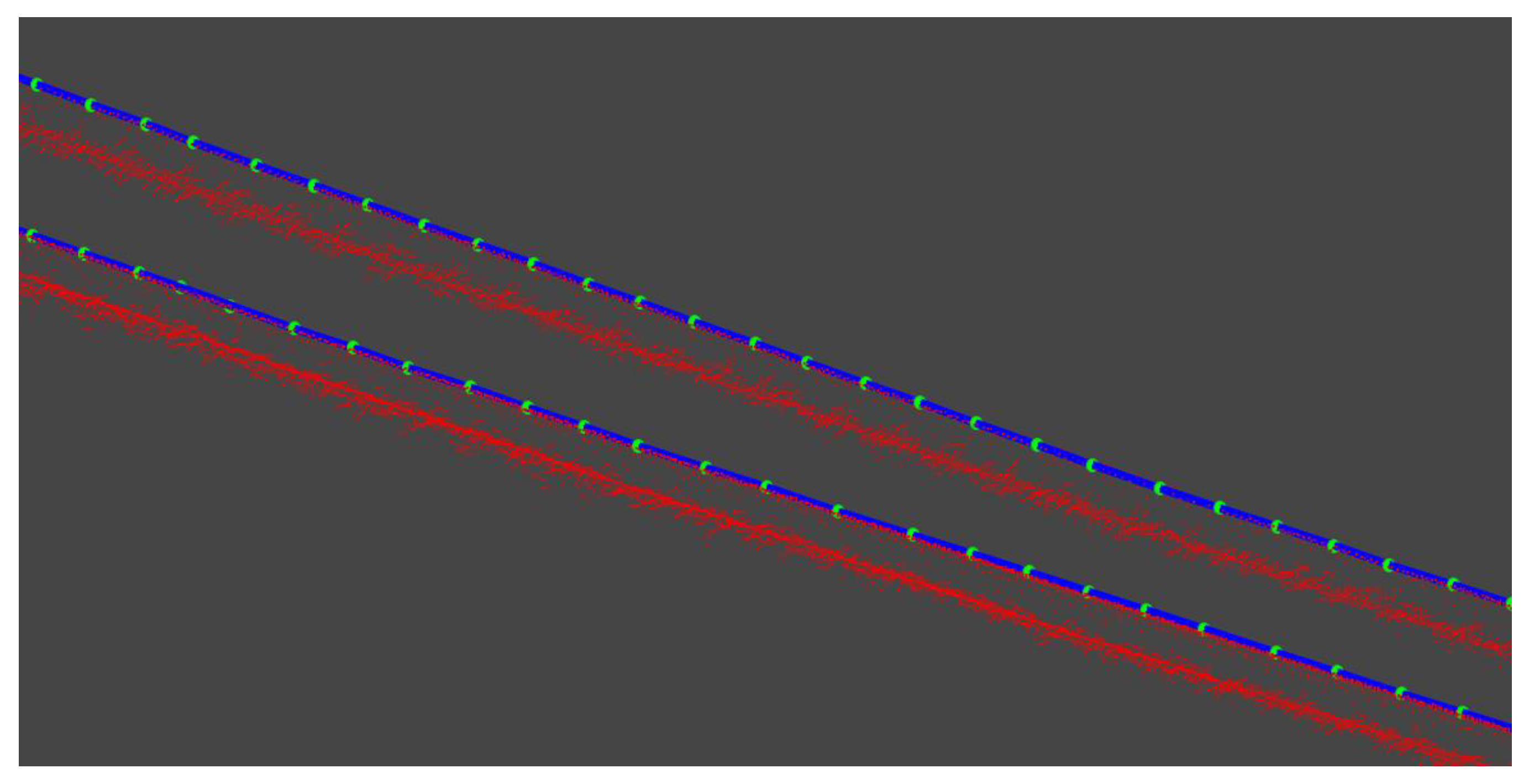
Rail tracks scan angle classified points and rail tracks top centre lines (blue) resulting from the vertices (green) union.
Figure 9.
Rail tracks scan angle classified points and rail tracks top centre lines (blue) resulting from the vertices (green) union.

Figure 10.
Scan angle coloured point cloud cross-section, with ballast top and bottom indication.

Figure 11.
Scan angle top and bottom ballast points classification (red).

Figure 12.
Resulting ballast top (blue) and bottom (green) extracted lines.

Figure 13.
Elevation coloured point cloud obtained after data processing.

Figure 14.
Highlighted area of total line’s extraction.

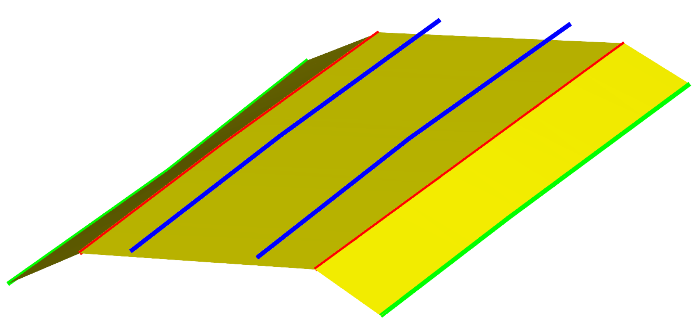
Figure 15.
Three-dimensional linear elements modelling sample.


Table 1.
Riegl VQ-250 sensor main characteristics.
| Characteristics | Values |
|---|---|
| Scan frequency | 200 Hz |
| Laser pulse repetition rate | Up to 300 Hz |
| Minimum distance | 1.5 m |
| Points relative precision | 0.005 m |
Table 2.
Three-dimensional extracted lines accuracy measurements.
| Extracted Line | Completeness (%) | Correctness (%) | Quality (%) |
|---|---|---|---|
| Left bottom ballast | 82.0 | 81.6 | 69.2 |
| Left top ballast | 85.8 | 85.4 | 74.8 |
| Right bottom ballast | 80.6 | 80.4 | 67.3 |
| Right top ballast | 82.9 | 82.5 | 70.5 |
| Left rail | 98.7 | 98.9 | 97.7 |
| Right rail | 99.3 | 99.3 | 98.6 |
© 2019 by the authors. Licensee MDPI, Basel, Switzerland. This article is an open access article distributed under the terms and conditions of the Creative Commons Attribution (CC BY) license (http://creativecommons.org/licenses/by/4.0/).
Share and Cite
MDPI and ACS Style
Gézero, L.; Antunes, C. Automated Three-Dimensional Linear Elements Extraction from Mobile LiDAR Point Clouds in Railway Environments. Infrastructures 2019, 4, 46. https://0-doi-org.brum.beds.ac.uk/10.3390/infrastructures4030046
AMA Style
Gézero L, Antunes C. Automated Three-Dimensional Linear Elements Extraction from Mobile LiDAR Point Clouds in Railway Environments. Infrastructures. 2019; 4(3):46. https://0-doi-org.brum.beds.ac.uk/10.3390/infrastructures4030046
Chicago/Turabian StyleGézero, Luis, and Carlos Antunes. 2019. "Automated Three-Dimensional Linear Elements Extraction from Mobile LiDAR Point Clouds in Railway Environments" Infrastructures 4, no. 3: 46. https://0-doi-org.brum.beds.ac.uk/10.3390/infrastructures4030046