Tracking the 6-DOF Flight Trajectory of Windborne Debris Using Stereophotogrammetry

Abstract

Numerous post-windstorm investigations have reported that windborne debris can cause costly damage to the envelope of buildings in urban areas under strong winds (e.g., during hurricanes or tornados). Thus, understanding the physics of debris flight is of critical importance. Previously developed numerical models describing debris flight physics have not been validated for the complex urban flow environment; such a validation requires experimentally measuring the debris flight trajectory in wind tunnel tests. In this context, this paper proposes a debris measurement algorithm using stereophotogrammetry. This algorithm aims to determine the six-degree-of-freedom (6-DOF) trajectory and velocity of flying debris, addressing the research gap, i.e., the lack of an algorithm/software for measuring three-rotational-DOF using stereophotogrammetry. This is a civil engineering problem, but computer graphics is the foundation to solve it. This paper focuses on the theoretical development of the algorithm. The developed algorithm can be readily implemented in modern wind tunnel experiments.

1. Introduction

Windborne debris damage to the cladding and façades of buildings has been identified as a major contributor to damage in urban areas after windstorms (e.g., hurricanes, tornados, thunderstorms) in numerous studies [1,2,3,4,5,6,7,8,9,10,11]. To physically model debris-induced damage, one needs to understand debris flight behavior. In recent years, there have been a number of experimental and numerical studies investigating the mechanics of debris flight. Tachikawa [12] pioneered fundamental research on the two-dimensional (2D) trajectory of a flying plate in a uniform flow through both wind tunnel experiments and numerical simulation. Following Tachikawa’s work, Lin et al. [13,14] conducted wind tunnel studies to investigate the trajectories of compact-, rod-, and plate-type debris in a uniform wind field and provided experimental support for the validation of numerical simulations using Tachikawa’s equations. However, the numerical models developed in the literature have not been validated for the complex 3D urban wind field. Researchers have found that a complex turbulent flow structure in an urban environment can dramatically alter the typical flight distance/speed and lead to unusual debris trajectory, through both experimental and full-scale investigations [15,16,17,18]. Thus, experimental validation of the numerical debris flight model for an urban built environment is critical for understanding complex debris flight behavior and predicting the debris impact location, energy/momentum, and ultimately the damage state of the building envelope components. Such a validation first requires the measurement of the debris flight trajectory in a 3D field in wind tunnel tests. In the hardware aspect, the high-speed cameras that have become more accessible in modern wind tunnels can be used for the measurement; however, to the authors’ knowledge, there is no off-the-shelf algorithm/software for extracting the entire six-degree-of-freedom (6-DOF) trajectory of flying debris from the images. The existing literature on trajectory measuring of windborne debris using high-speed cameras either only measures the three-translational-DOF (without the three-rotational-DOF) [19] or qualitatively analyzes the different flight modes of the debris instead of resolving the coordinates of the full trajectory [17]. In this context, this paper proposes a debris trajectory measuring algorithm that can reconstruct all 6-DOF displacements and the velocity of debris in a 3D field from pairs of stereoscopic 2D images captured by two high-speed, high-resolution cameras. The concept of using pairs of stereoscopic 2D images to track debris is similar to stereoscopic particle image velocimetry (PIV), which is a non-intrusive laser optical technique for measurement of flow velocity. However, it is distinct from stereoscopic PIV in the following three aspects: (i) the proposed method tracks a single piece of debris, while PIV tracks the patterns of a group of flow particles; (ii) the proposed method does not rely on a laser sheet to illuminate the debris, and thus can track the debris flight with larger lateral motion, while PIV can only track particle motions within the thickness of a laser sheet; and (iii) the proposed method is developed to track the 6-DOF trajectory of debris, while PIV can only measure the 3-DOF motions of flow particles. In wind engineering, three types of debris are typically concerned, i.e., compact, rod, and thin plate. In this paper, we focus on the thin plate. The theoretical development of the three-translational-DOF of compact debris has been included in this discussion as the foundation for the algorithm for thin plates. Furthermore, this algorithm can be extended to consider rod-like debris in the future.

The paper is organized as follows. Section 2 includes the problem formulation and notation. Section 3 focuses on the reconstruction of the 6-DOF coordinates of debris from stereopairs of camera images. Section 4 derives the differential operator for velocity reconstruction. Section 5 introduces procedures for the reconstruction of time histories of debris motion trajectory, including both displacements and velocity. Section 6 includes concluding remarks and a discussion of future directions.

2. Background

Problem Formulation and Notation

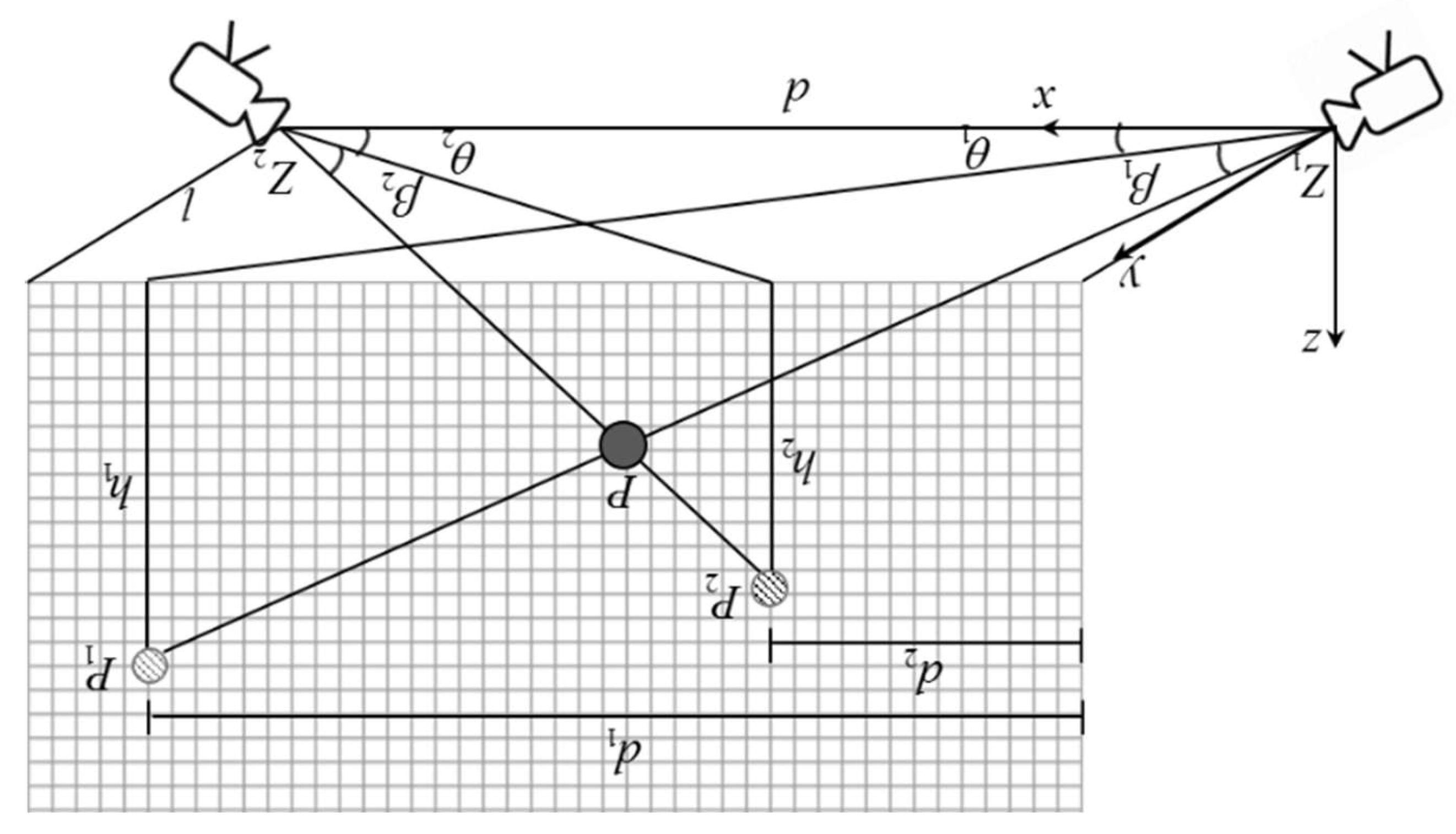
In this problem (depicted in Figure 1), first, a background grid is utilized to calibrate the corresponding pixel locations for two high-speed cameras; it can be removed once the calibration is completed. Then the two cameras are used to measure the 2D coordinates of the projection of flying debris on the grid wall by lights emanating from the camera locations. Using the stereopair of 2D coordinates (i.e., $d_1$, $h_1$, $d_2$, $h_2$ measured by the two cameras) of the debris, we try to determine both the position (three-translational-DOF, x, y, z) and orientation (three-rotational-DOF) of the debris, given the relative locations of the two cameras to the grid wall (i.e., $d$ and $l$).

This problem will be solved in two steps: First, for a single compact piece of debris, considered as a point object (only three-translation-DOF is considered), then for rigid body thin plate debris. The former lays the theoretical foundation for the latter.

The notation used in the problem is defined as follows. The notation of points and matrices are in upper case letters, the position vectors are in bold lowercase letters, and vectors are column vectors by default. For example, $z_j$ is the position vector of point $Z_j$, while $p_j$ is the position vector of point $P_j$. The list of variables used in Figure 1 is given below.

$Z_1$, $Z_2$	–points at the lens positions of two cameras
$P$	–position of a point debris
$P_1$, $P_2$	–projected locations of the debris on the grid wall seen from two cameras (i.e., a stereopair), respectively
$d$	–distance between cameras
$l$	–distance between camera lens and the wall along the y-direction; the wall is parallel to the z‒x plane
$d_1$, $d_2$	–distances of points on the wall along the x-axis from the y-axis
$h_1$, $h_2$	–heights of points on the wall along the z-axis from the x‒y plane
${\beta }_1$, ${\beta }_2$	–angles that $Z_1{P}_1$, $Z_2{P}_2$ rays make with the x‒y plane
${\theta }_1$, ${\theta }_2$	–angles between the x-axis and the projections of $Z_1{P}_1$, $Z_2{P}_2$ rays on the x‒y plane

We need to determine the 3D position of the debris, i.e., x, y, and z, in terms of these parameters.

3. Debris Position and Spatial Orientation (6-DOF) in 3D Space

3.1. The 2D Stereopairs’ Positions

In Figure 1, $Z_1$ is the origin and $Z_2$ is the origin offset by $d$ units along the x-axis: $z_2=z_1+{[d,0,0]}^T$. The position vector for point $P_1$ on the wall is

$$p_1={[h_1\cot ({\beta }_1)\cos ({\theta }_1),h_1\cot ({\beta }_1)\sin ({\theta }_1),h_1]}^T,$$

(1)

with a distance from $Z_1$ of:

$$t_1=h_1 \cos \mathrm{ec}({\beta }_1)=\left|C_1{P}_1\right|.$$

(2)

Alternatively, $p_1=\left[d_1,d_1\tan ({\theta }_1),h_1\right]$, $t_1=\sqrt{d_1{}^2\sec {({\theta }_1)}^2+h_1{}^2}$. Similarly, for point $P_2$ on the wall:

$$p_2={\left[d_1,0,0\right]}^T+{\left[-h_2\cot ({\beta }_2)\cos ({\theta }_2),h_2\cot ({\beta }_2)\sin ({\theta }_2),h_2\right]}^T,$$

(3)

with a distance from $Z_2$ of:

$$t_2=h_2 \cos \mathrm{ec}({\beta }_2)=\left|Z_2{P}_2\right|.$$

(4)

Alternatively,

$$\begin{gathered} \begin{array}{l}{p}_2={\left[d,0,0\right]}^T+{\left[-(d-d_2),(d-d_2)\tan ({\theta }_2),h_2\right]}^T\\ \\ ={\left[d_2,(d-d_2)\tan ({\theta }_2),h_2\right]}^T\end{array} \end{gathered}$$

(5)

$$t_2=\sqrt{{(d-d_2)}^2 \cos \mathrm{ec}({\theta }_2{)}^2+h_2^2}.$$

(6)

In the simplest terms, the vectors along $Z_1{P}_1$ and $Z_2{P}_2$ are normalized to unit vectors, $d_1$ and $d_2$, where

$$d_1={\left[\cos ({\beta }_1)\cos ({\theta }_1),\cos ({\beta }_1)\sin ({\theta }_1),\sin ({\beta }_1)\right]}^T$$

(7)

$$d_2={\left[-\cos ({\beta }_2)\cos ({\theta }_2),\cos ({\beta }_2)\sin ({\theta }_2),\sin ({\beta }_2)\right]}^T.$$

(8)

Then the position vectors for the stereo-pair $P_1$ and $P_2$ are

$$p_1=z_1+t_1{d}_1, p_2=z_2+t_2{d}_2.$$

(9)

This is valid even if the cameras are not at the same distance from the wall.

3.2. The Relationship between the 3D Spatial Position of Debris and the 2D Stereopairs’ Positions

Consider compact debris or a point object. The camera beams intersect at the true location of the debris in 3D space with position vector: $z_1+s_1{d}_1=z_2+s_2{d}_2$. This leads to the following equations:

$$s_1{d}_1-s_2{d}_2=z_2-z_1$$

(10)

$$\left[d_1,-d_2\right]\left[\begin{array}{c}{s}_1\\ s_2\end{array}\right]=z_2-z_1.$$

(11)

This is an overdetermined system of three equations involving two unknowns, $s_1$ and $s_2$. Let $M=\left[d_1\hspace{1em}-d_2\right]$, which is a 3 $\times$ 2 matrix. Since a 3 $\times$ 2 matrix does not have an inverse, we exploit the generalize inverse, denoted by $M^{+}$, to determine the least squares error solution. Now $M^T=\left[\begin{array}{c}{d}_1^T\\ -d_2^T\end{array}\right]$ it is a 2 $\times$ 3 matrix, so we create a 2$\times$ 2 matrix, $M^{T}M$:

$$M^{T}M=\left[\begin{array}{c}{d}_1^T\\ -d_2^T\end{array}\right]\left[d_1^T,-d_2^T\right]=\left[\begin{array}{cc}{d}_1^T{d}_1& -d_1^T{d}_2\\ -d_2^T{d}_1& d_2^T{d}_2\end{array}\right]=\left[\begin{array}{cc}{d}_1\cdot d_1& -d_1\cdot d_2\\ -d_1\cdot d_2& d_2\cdot d_2\end{array}\right].$$

(12)

Since $d_1$ and $d_2$ are unit vectors, let $k=d_1\cdot d_2=\cos (\theta )$, where $\theta$ is the angle between $d_1$ and $d_2$. Then,

$$M^{T}M=\left[\begin{array}{cc}1& -k\\ -k& 1\end{array}\right], \det (M^{T}M)=1-k^2$$

$$M^{+}={(M^{T}M)}^{-1}{M}^T=\frac{\left[\begin{array}{cc}1& k\\ k& 1\end{array}\right]}{1-k^2}\left[\begin{array}{c}{d}_1^T\\ -d_2^T\end{array}\right], M^{+}=\frac{\left[\begin{array}{c}{d}_1^T-k{d}_2^T\\ k{d}_1^T-d_2^T\end{array}\right]}{1-k^2}$$

(13)

Then,

$$\left[\begin{array}{c}{s}_1\\ s_2\end{array}\right]={\left[d_1,-d_2\right]}^{+}(z_2-z_1)=\frac{\left[\begin{array}{c}{d}_1^T-k{d}_2^T\\ k{d}_1^T-d_2^T\end{array}\right]}{1-k^2}(z_2-z_1).$$

(14)

This form is useful when the camera direction changes and the location is fixed; otherwise, it can be further simplified to

$$\left[\begin{array}{c}{s}_1\\ s_2\end{array}\right]=\frac{\left[\begin{array}{c}(d_1^T-k{d}_2^T)(z_2-z_1)\\ (k{d}_1^T-d_2^T)(z_2-z_1)\end{array}\right]}{1-k^2}.$$

(15)

We computed vector forms $z_1+t_1{d}_1$, $z_2+t_2{d}_2$ for input points on the wall. Now we have computed $\left[\begin{array}{c}{s}_1\\ s_2\end{array}\right]$ for the corresponding object in 3D space. The actual object is at $z_1+s_1{d}_1=z_2+s_2{d}_2$ for these $s_1$ and $s_2$. This suggests that the object size at $z_1+t_1{d}_1$ can be scaled by $\frac{s_1}{t_1}$, with $s_1$ computed above, along direction $d_1$ to get the actual size at $z_1+s_1{d}_1$ in 3D space. Similarly, for camera 2, the object size at $z_2+t_2{d}_2$ is scaled by $\frac{s_2}{t_2}$, ($s_2$ computed above), along the direction $d_2$_. The rationale for the scaling of an object at $P_1$ by a scale factor of $\frac{s_1}{t_1}$ along the line $Z_1{P}_1$ is as follows:

$$z_1+\frac{s_1}{t_1}(Z_1{P}_1)=z_1+\frac{s_1}{t_1}(p_1-z_1)\hspace{0.17em}=z_1+\frac{s_1}{t_1}(z_1+t_1{d}_1-z_1)=z_1+\frac{s_1}{t_1}(t_1{d}_1)=z_1+s_1{d}_1.$$

(16)

Similarly, for camera 2,

$$z_2+\frac{s_2}{t_2}(Z_2{P}_2)=z_2+s_2{d}_2.$$

(17)

3.3. Explicit Expressions of Debris Position in 3D Space

Once $s_1$ is determined for 3D position, we can compute the desired parameters x, y, and z as in Figure 1. Now $s_1{d}_1$ becomes

$$s_1{d}_1={\left[z\cot ({\beta }_1)\cos ({\theta }_1),z\cot ({\beta }_1)\sin ({\theta }_1),z\right]}^T.$$

(18)

Since $d_1$ is a unit vector, this implies that

$$s_1=z \cos \mathrm{ec}({\beta }_1), z=s_1\sin ({\beta }_1), r_1=s_1\cos ({\beta }_1)$$

$$x=r_1\cos ({\theta }_1)=s_1\cos ({\beta }_1)\cos ({\theta }_1), y=r_1\sin ({\theta }_1)=s_1\cos ({\beta }_1)\sin ({\theta }_1).$$

(19)

Similarly,

$$s_2=z \cos \mathrm{ec}({\beta }_2),z=s_2\sin ({\beta }_2),r_2=s_2\cos ({\beta }_2)$$

$$x=d_1-r_2\cos ({\theta }_2)=d_1-s_2\cos ({\beta }_2)\cos ({\theta }_2), y=r_2\sin ({\theta }_2)=s_2\cos ({\beta }_2)\sin ({\theta }_2).$$

(20)

3.4. Cartesian Position and Orientation for Thin Plate Debris

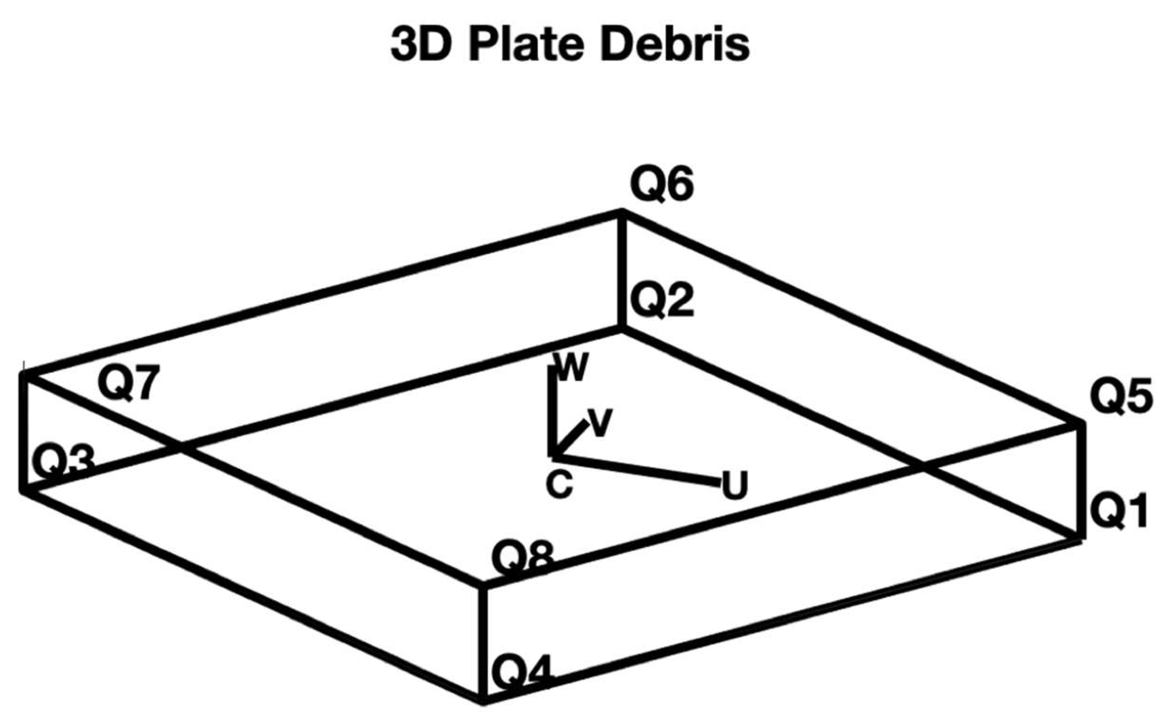
Now we derive the position and orientation for rigid body thin plate debris, based on the 3D positions of the point objects constructed from the stereo images in the previous section. In Figure 2, let $C$ be the centroid (also called the pivot) of the rigid body plate with vertices $Q_1$, $Q_2$, $Q_3$, $Q_4$, $Q_5$, $Q_6$, $Q_7$, and $Q_8$. Assume that the vertices of the debris are identifiable in the stereo images using marker tracking. The 3D positions of the vertices can then be determined using the expressions in the previous section based on the stereo measurements. The problem now becomes using the 3D positions of vertices to determine the orientation (three-rotational-DOF) of the rigid body.

Firstly, a local coordinate system needs to be defined using any three non-collinear points on the debris. Here we use the points $C$, $Q_1$, and $Q_2$ to create a local coordinate system centered at $C$ and axis directions with unit vectors $u$, $v$, and $w$, where $u$ is along $C{Q}_1$, $v$ is orthogonal to $C{Q}_1$ and in the plane of $C$, $Q_1$, and $Q_2$, with a projection of $C{Q}_2$ on $v$ positive, and $w$ is naturally $u\times v$ so that $u$, $v$, and $w$ form a right-handed system of orthonormal vectors: $u=\frac{C{Q}_1}{\left|C{Q}_1\right|}$, $v=\frac{C{Q}_2-u\cdot C{Q}_{2}u}{\left|C{Q}_2-u\cdot C{Q}_{2}u\right|}$, $w=u\times v$ (equivalently $w=\frac{u\times C{Q}_2}{\left|u\times C{Q}_2\right|}$, $v=w\times u$).

The matrix $R=\left[\begin{array}{ccc}u& v& w\end{array}\right]$ of axis unit vectors is the rotation matrix and is just the 3D local coordinate system at $C$. For simplicity in the notation for time history of the plate trajectory determined from vertices reconstructed using stereopairs, the 3D plate is represented as a frame $F(t)$ at time $t$ that contains both the position and the orientation for the plate. Since at each time point of the trajectory, there is a frame, the frame sequence will later be denoted by $F_k$, $k=1,2,\dots ,N$. This is similar to frames in a robotic system of $N$- links.

The matrix $F=\left[\begin{array}{cc}R& c\\ 0& 1\end{array}\right]$ represents the local coordinate system centered at $C$. The frame can be written interchangeably as

$$F=\left[\begin{array}{cc}R& c\\ 0& 1\end{array}\right]=\left[\begin{array}{c}\begin{array}{cccc}u& v& w& c\end{array}\\ \begin{array}{cccc}0& 0& 0& 1\end{array}\end{array}\right]=\left[\begin{array}{cccc}{u}_1& v_1& w_1& c_1\\ u_2& v_2& w_2& c_2\\ u_3& v_3& w_3& c_3\\ 0& 0& 0& 1\end{array}\right].$$

(21)

This matrix $F$ transforms $\left[\begin{array}{c}\begin{array}{cccc}i& j& k& 0\end{array}\\ \begin{array}{cccc}0& 0& 0& 1\end{array}\end{array}\right]$ to $\left[\begin{array}{c}\begin{array}{cccc}u& v& w& c\end{array}\\ \begin{array}{cccc}0& 0& 0& 1\end{array}\end{array}\right]$. The inverse of $F$ transforms the coordinate system $\left[\begin{array}{c}\begin{array}{cccc}u& v& w& c\end{array}\\ \begin{array}{cccc}0& 0& 0& 1\end{array}\end{array}\right]$, located at the centroid $C$ of the debris, to the universal coordinate system $\left[\begin{array}{c}\begin{array}{cccc}i& j& k& 0\end{array}\\ \begin{array}{cccc}0& 0& 0& 1\end{array}\end{array}\right]$. The inverse of $F$ can be written as follows:

$$F^{-1}=\left[\begin{array}{cc}\begin{array}{c}{u}^T\\ v^T\\ w^T\\ 0\end{array}& \begin{array}{c}-u^{T}c\\ -v^{T}c\\ -w^{T}c\\ 1\end{array}\end{array}\right]=\left[\begin{array}{cccc}{u}_1& v_1& w_1& -u^{T}c\\ u_2& v_2& w_2& -v^{T}c\\ u_3& v_3& w_3& -w^{T}c\\ 0& 0& 0& 1\end{array}\right]\hspace{0.17em}=\left[\begin{array}{cccc}{u}_1& v_1& w_1& -(u_1{c}_1+u_2{c}_2+u_3{c}_3)\\ u_2& v_2& w_2& -(v_1{c}_1+v_2{c}_2+v_3{c}_3)\\ u_3& v_3& w_3& -(w_1{c}_1+w_2{c}_2+w_3{c}_3)\\ 0& 0& 0& 1\end{array}\right].$$

(22)

3.5. Three-Degree-of-Freedom (3-DOF) Frames in Universal Coordinate System

Here we describe the relationship between the local coordinate system and the axis of rotation and the amount of rotation in a universal coordinate system. The local coordinate system at the centroid of the plate is a frame

$$F=\left[\begin{array}{cc}R& c\\ 0& 1\end{array}\right]=\left[\begin{array}{c}\begin{array}{cccc}u& v& w& c\end{array}\\ \begin{array}{cccc}0& 0& 0& 1\end{array}\end{array}\right],$$

(23)

where $R$ is the rotation matrix about an axis, which is a composite of rotations about the x, y, and z axes. If $n$ is the unit vector and $\theta$ is the angle amount of counter clockwise rotation about $n$, the axis through the origin, then [20]

$$R=n{n}^T+(I-n{n}^T)\cos (\theta )+n\times I\sin (\theta ).$$

(24)

This is directly related to the matrix representation, $R=\left[\begin{array}{ccc}u& v& w\end{array}\right]$. The angle $\theta$ and vector $n$ are given by

$$\theta ={\cos }^{-1}(\frac{u_1+v_2+w_3-1}{2})$$

(25)

$$n=\left[\begin{array}{c}{n}_1\\ n_2\\ n_3\end{array}\right]=\left[\begin{array}{c}{v}_3-w_2\\ w_1-u_3\\ u_2-v_1\end{array}\right]/2\sin (\theta ).$$

(26)

The rotation vector and amount of rotation about $n$ is denoted by $n\theta$, giving the 3-DOF Euler angles, components of rotation about the x, y, and z axes in the universal coordinate system.

3.6. Differential Operators for 6-DOF Motion

To facilitate the determination of the velocity, differential operators for 6-DOF motion with respect to the universal coordinate system are derived in this section. Let $dF=F_{k+1}-F_k$ or explicitly 3-DOF translational and 3-DOF rotational differentials are

$$dF=\left[\begin{array}{cc}dR& dc\\ 0& 0\end{array}\right],$$

(27)

where $dR$ and $dc$ are differential changes in rotation ($R$) and translation ($c$). The differential $dc$ is a linear differential in the x, y, and z coordinates of $c$; it is simple and trivial. However, differential change, $dR$, in the angle of rotation is not straightforward because the differential of the rotation matrix is a matrix operator. Recall that matrix $R$ [21] is

$$R=n{n}^T+(I-n{n}^T)\cos (\theta )+n\times I\sin (\theta ).$$

(28)

Differentiating with respect to $\theta$, we have

$$dR/d\theta =-(I-n{n}^T)\sin (\theta )+n\times I\cos (\theta ).$$

(29)

This derivative of the rotation matrix can be expressed as a matrix multiplication, the differential operator [21]. This is accomplished by cross-multiplying Equation (28) by $n$ as follows:

$$n\times R=n\times (n{n}^T+(I-n{n}^T)\cos (\theta )+n\times I\sin (\theta )).$$

(30)

Using vector manipulation identities, this convoluted expression is simplified as follows:

$$\begin{gathered} \begin{array}{l}n\times R=n\times n{n}^T+n\times (I-n{n}^T)\cos (\theta )+n\times (n\times I)\sin (\theta )=0+(n\times I-0)\cos (\theta )+(nn\cdot I-In\cdot n)\sin (\theta )\\ \\ =n\times I\cos (\theta )+(n{n}^T-I)\sin (\theta )=-(I-n{n}^T)\sin (\theta )+n\times I\cos (\theta )\end{array} \end{gathered}$$

(31)

which is identical to $dR/d\theta$, as obtained in Equation (29).

Recalling that the amount of rotation in the universal coordinate system is represented by $\theta n$, the differential becomes $d\theta n$, which yields the rotation about the x, y, and z axes. This is consistent with the differential operator derived from the matrix:

$$dR/d\theta =n\times R=n\times IR,$$

$$dR=n\times Rd\theta =n\times IRd\theta =n\times Id\theta R=nd\theta \times IR=\Delta R,$$

(32)

where $\Delta$ is the differential operator, defined below. Thus, the differential $dR$ of $R$ is a matrix multiplication of $R$ by a matrix, called the differential operator and denoted by $\Delta$.

$$\Delta =nd\theta \times I=\left[\begin{array}{ccc}0& -d\theta n_3& d\theta n_2\\ d\theta n_3& 0& -d\theta n_1\\ -d\theta n_2& d\theta n_1& 0\end{array}\right], \mathrm{or} \mathrm{simply} =\left[\begin{array}{ccc}0& -d{\theta }_z& d{\theta }_y\\ d{\theta }_z& 0& -d{\theta }_x\\ -d{\theta }_y& d{\theta }_x& 0\end{array}\right].$$

(33)

Summarizing, if $\theta$ is the angle of rotation about $n$ and $\theta n$ represents the amount of rotation in the universal coordinate system, then the differential becomes $d\theta n$, which yields the rotation about the x, y, and z axes; it is consistent with the differential operator derived from the matrix. Here $\Delta$ is the differential operator that represents the differential change from $R_k$ to $R_{k+1}$ with respect to the universal coordinate system, where $R_k$ is the rotational submatrix of frame $F_k$. The rotational part is $\left[\begin{array}{ccc}0& -d{\theta }_z& d{\theta }_y\\ d{\theta }_z& 0& -d{\theta }_x\\ -d{\theta }_y& d{\theta }_x& 0\end{array}\right]$ with the angular changes about the x, y, and z axes. In short, the rotational differential is ${\left[\begin{array}{ccc}d{\theta }_x& d{\theta }_y& d{\theta }_z\end{array}\right]}^T$ and the translational differential is ${\left[\begin{array}{ccc}dx& dy& dz\end{array}\right]}^T$. The composite differential is 6-DOF vector ${\left[\begin{array}{cccccc}dx& dy& dz& d{\theta }_x& d{\theta }_y& d{\theta }_z\end{array}\right]}^T$, representing a composite vector for the translational and rotational velocity about the x, y, and z axes, similar to the notation used in Jacobians for the velocity of robotic link velocity applications.

4. 6-DOF Motion Consideration

4.1. Motivation

It is not necessary to know the initial velocity in this case; only the differential change matters. At any time $t$, from the position of the plate, we can get the orientation from the frame $F(t)$. Also, during the motion, some features invisible to the camera may become visible, while some that are visible may become invisible. We need to identify at least three vertices, which will be flagged at all times for the sake of calculating the local coordinate system and the rotational motion, in addition to the translational motion.

As the debris moves, frame $F(t)$ at time $t$ moves to the next frame $F(t+h)$ with time step $h$; the differential change in the frame, denoted by $dF=F(t+h)-F(t)$, can be used to derive the numerical instantaneous translational and rotational velocities. In this case, the debris is flying behind a building; the average velocity can be derived from visible positions (after the time lag of the hidden period) or continuously from the flags identified earlier. In such cases, we may opt to have one continuous trajectory, or multiple segments of trajectory.

4.2. The Relationship between Differential Transformations in Universal and Local Coordinate Systems

4.2.1. General Transformation

As a transformation is accomplished using two coordinate systems, the transformation can be expressed between them in terms of universal and local coordinate systems. In general, if $T$ is the transformation of frame $F$ with respect to the universal coordinate system, this is represented by U, while $T{}^{\prime }$ is its counterpart in the local coordinate system. They are related by the equation $T=FT{}^{\prime }{F}^{-1}$. If a point or matrix $X$ has coordinates with respect to frame $F$, then $TF\left(X\right)=F\left(T{}^{\prime }\left(X\right)\right)$. Equivalently, if $Y$ has coordinates with respect to the universal frame, then $T\left(Y\right)=F\left(T{}^{\prime }\left(F^{-1}\left(Y\right)\right)\right)$. Thus, $T$ and $T{}^{\prime }$ accomplish the same task from different coordinate systems, and are related by the equations $T=FT{}^{\prime }{F}^{-1}$ and $T{}^{\prime }=F^{-1}TF$.

4.2.2. Rotational Differential Transform with Respect to Universal Coordinate System

We have shown that for rotation matrix $R$, the rotation differential operator with respect to the universal coordinate system is $\Delta =nd\theta \times I$. Let $\omega =nd\theta$ be called the angular differential, then $\Delta =\omega \times I$.

4.2.3. Differential Transform in Universal Coordinate System

The translational and rotational velocities are first computed in the universal coordinate system.

Definition 1.

For$F=\left[\begin{array}{cc}R& c\\ 0& 1\end{array}\right]$and the universal differential transformation matrix$T$, the differential change in frames is defined as follows:

$$dF=TF=\left[\begin{array}{cc}dR& dc\\ 0& 0\end{array}\right]=\left[\begin{array}{cc}\Delta R& dc\\ 0& 0\end{array}\right],$$

(34)

where$\Delta =\omega \times I$, $\omega =n\mathrm{d}\theta$, $dc=\left[\begin{array}{c}dx\\ dy\\ dz\end{array}\right]$.

Now we define $T$ as the differential operator with respect to the universal coordinate system. $dF=TF$ implies $T=dF{F}^{-1}$, then $T=\left[\begin{array}{cc}\Delta & dc-\Delta c\\ 0& 0\end{array}\right]$.

4.2.4. Differential Transform in Local Coordinate System

For studying the different flight modes of a plate, it is desirable to have the computation of velocities also available in the local coordinate system, and is more conceptually reasonable. Before deriving the differential transformation in the local coordinate system, we will first show a few auxiliary results.

• Show that the rotation differential operator $\Delta {}^{\prime }=R^T\Delta R$ with respect to the local frame system, such that

  $$\Delta {}^{\prime }=\left[\begin{array}{c}\omega \cdot u\\ \omega \cdot v\\ \omega \cdot w\end{array}\right]\times I.$$

  (35)
  Proof. 

  $$\Delta {}^{\prime }=R^T\Delta R=R^T\omega \times IR=R^T\omega \times R=R^T\left[\omega \times u,\omega \times v,\omega \times w\right]=\left[R^T\omega \times u,R^T\omega \times v,R^T\omega \times w\right]$$

  $$=\left[\left[\begin{array}{c}\omega \times u\cdot u\\ \omega \times u\cdot v\\ \omega \times u\cdot w\end{array}\right],\left[\begin{array}{c}\omega \times v\cdot u\\ \omega \times v\cdot v\\ \omega \times v\cdot w\end{array}\right],\left[\begin{array}{c}\omega \times w\cdot u\\ \omega \times w\cdot v\\ \omega \times w\cdot w\end{array}\right]\right]=\left[\begin{array}{ccc}0& -\omega \cdot w& \omega \cdot v\\ \omega \cdot w& 0& -\omega \cdot u\\ -\omega \cdot v& \omega \cdot u& 0\end{array}\right]=\left[\begin{array}{c}\omega \cdot u\\ \omega \cdot v\\ \omega \cdot w\end{array}\right]\times I.$$

   □
• Show that the linear differential $dc{}^{\prime }=R^{T}dc$ in the local frame simplifies to

  $$dc{}^{\prime }=\left[\begin{array}{c}dc\cdot u\\ dc\cdot v\\ dc\cdot w\end{array}\right].$$

  (36)
  Proof. 

  $$dc{}^{\prime }=R^{T}dc=\left[\begin{array}{c}{u}^T\\ v^T\\ w^T\end{array}\right], dc=\left[\begin{array}{c}{u}^{T}dc\\ v^{T}dc\\ w^{T}dc\end{array}\right]=\left[\begin{array}{c}u\cdot dc\\ v\cdot dc\\ w\cdot dc\end{array}\right]=\left[\begin{array}{c}dc\cdot u\\ dc\cdot v\\ dc\cdot w\end{array}\right].$$

  (37)

   □
• Differential operator with respect to local frame coordinate system.
  Theorem 1.

  The frame differential transformation matrix$T{}^{\prime }$in the local coordinate system is

  $$T{}^{\prime }=\left[\begin{array}{cc}\Delta {}^{\prime }& dc{}^{\prime }\\ 0& 0\end{array}\right],$$

  (38)

  where$\Delta {}^{\prime }=\left[\begin{array}{c}\omega \cdot u\\ \omega \cdot v\\ \omega \cdot w\end{array}\right]\times I$, $dc{}^{\prime }=\left[\begin{array}{c}dc\cdot u\\ dc\cdot v\\ dc\cdot w\end{array}\right]$.

  Proof. 

  From $T{}^{\prime }=F^{-1}TF$ (Section 4.2.1) and $TF=\left[\begin{array}{cc}\Delta R& dc\\ 0& 0\end{array}\right]$ (Equation (34)), we get

  $$\begin{gathered} T{}^{\prime }=\left[\begin{array}{cc}{R}^T& -R^{T}c\\ 0& 1\end{array}\right]\left[\begin{array}{cc}\Delta R& dc\\ 0& 0\end{array}\right]=\left[\begin{array}{cc}{R}^T\Delta R& R^{T}dc\\ 0& 0\end{array}\right]=\left[\begin{array}{cc}\Delta {}^{\prime }& dc{}^{\prime }\\ 0& 0\end{array}\right] \\ (\mathrm{recall} \mathrm{that} \Delta {}^{\prime }=R^T\Delta R \mathrm{and} dc{}^{\prime }=R^{T}dc). \end{gathered}$$

  (39)

  Hence, the theorem is proved. □

Finally, the 6-DOF local translational and rotational velocities in the local frame are derived from the differential transformation as follows:

$$dF{}^{\prime }=T{}^{\prime }F=\left[\begin{array}{cc}\Delta {}^{\prime }& dc{}^{\prime }\\ 0& 0\end{array}\right]\left[\begin{array}{cc}R& c\\ 0& 1\end{array}\right]=\left[\begin{array}{cc}\Delta {}^{\prime }R& \Delta {}^{\prime }c+dc{}^{\prime }\\ 0& 0\end{array}\right].$$

(40)

5. 6-DOF Motion Trajectory with Velocity

5.1. Velocity

We have determined the 6-DOF frame for position and orientation, as well as the differentials for translational and rotational motion of the debris. High-speed, high-resolution cameras are fast enough to provide data on very small intervals of time. Assuming that the time history of 6-DOF frames has been reconstructed according to Section 3, we now determine the numerical derivatives from this sequence of 3D temporal positions and orientations (i.e., displacements) of the debris using the differentials derived in Section 4. This gives the translational and rotational velocities from the numerical time histories of the displacements.

5.2. Experimenting with 6DOF Position and Orientation and 6DOF Motion Methods

For the experiments, the data structure of debris is represented as a thin $m\times n\times q$ plate, where $m\times n$ is a polygonal face shape and $q$ is the thickness of the plate. The vertices of the plate are represented by a matrix array $deb=deb\left(x,y,z\right)$, where $x=x(1:m)$, $y=y(1:n)$, $z=z(1:q)$. For example, in Figure 2, with a 4 $\times$ 4 $\times$ 2 simple rectangular plate, we may define $z(1)=0$, $z(2)=2$, $x(1:4)=\left[1,50,50,1\right]$, $y(1:4)=[1,1,50,50]$; thus, one flat face is $face\hspace{0.17em}1=\left\{\left(x(k),y(k),z(1)\right);\hspace{1em}k=1,2,3,4\right\}$, and the second face is $face\hspace{0.17em}2=\left\{\left(x(k),y(k),z(2)\right);\hspace{1em}k=1,2,3,4\right\}$.

5.3. Implementation Procedure for Debris Tracking with Both Displacement and Velocity Time Histories Determined

Conceptual algorithms and implementation go hand in hand. From the stereopairs of images captured by two cameras, we computed the 3D spatial positions of flagged points on the debris. Then, using three non-collinear points (e.g., the centroid and two vertices), we constructed a frame matrix $F=\left[\begin{array}{cc}R& c\\ 0& 1\end{array}\right]$ to represent the position and orientation of the debris. Here $R=\left[\begin{array}{ccc}u& v& w\end{array}\right]$ represents the rotation matrix about unit vector $n$ through the origin by angle $\theta$, where $\theta ={\cos }^{-1}(\frac{u_1+v_2+w_3-1}{2})$ and $n=\left[\begin{array}{c}{v}_3-w_2\\ w_1-u_3\\ u_2-v_1\end{array}\right]/2\sin (\theta )$. $F$ changes its state over time as the debris moves. The motion trajectory is then captured by successive camera frames $F(t)$ to frame $F(t+h)$, where $h$ is the time step, depending on the camera speed. For translational and rotational velocity, we calculated the differential of frame $F$ as $dF=F(t+h)-F(t)=\left[\begin{array}{cc}dR& dc\\ 0& 1\end{array}\right]$, where $dc$ is the differential of centroids of frame $F(t)$ and subsequent frame $F(t+h)$, and $dR$ is the differential of orientation of frame $F(t)$ and subsequent frame $F(t+h)$. We have seen that $dR=\Delta R$ with $\Delta =\omega \times I$, $\omega =nd\theta$, $\mathrm{d}\theta ={\cos }^{-1}(\frac{u_1+v_2+w_3-1}{2})(t)-{\cos }^{-1}(\frac{u_1+v_2+w_3-1}{2})(t+h)$.

Now $dF$ can be written in terms of frame differential operator $T$ such that $dF=TF$, where $T=\left[\begin{array}{cc}\Delta & dc-\Delta c\\ 0& 0\end{array}\right]$.

Now for the trajectory of $N$ frames $F_k$, $k=1,2,\dots ,N$. Let the $k$th stereopair debris vertices be denoted by $Q_{k1i}=\left({}^{1}x_i,{}^{1}y_i,{}^{1}z_i\right)$, and $Q_{k2i}=\left({}^{2}x_i,{}^{2}y_i,{}^{2}z_i\right)$, $i=1,2,\dots ,8$.

The 3D spatial location corresponding to the points $Q_{k1i}$ and $Q_{k2i}$ is denoted by $P_{ki}$, whose position vector is $p_{ki}$.

Let $p_{ki}$ be the position vectors of vertices $P_{ki}$, and $c_k$ be the centroid of vertices $P_{ki}$ for $i=1,2,\dots ,8$.

Create frame $F_k$ with $u_k$, $v_k$, $w_k$, $c_k$ as follows:

$c_k=({\displaystyle {\sum }_{i=1,8}{p}_{ki})/8}$, $u_k=p_{k1}-c_k$, normalize $u_k=\frac{u_k}{\left|u_k\right|}$, $w_k=u_k\times (p_{k2}-c_k)$, normalize $w_k=\frac{w_k}{\left|w_k\right|}$

$$v_k=w_k\times u_k,{\theta }_k={\cos }^{-1}(\frac{u_{k1}+v_{k2}+w_{k3}-1}{2}), n_k=\left[\begin{array}{c}{v}_{k3}-w_{k2}\\ w_{k1}-u_{k3}\\ u_{k2}-v_{k1}\end{array}\right]/2\sin ({\theta }_k)$$

$$d{\theta }_k={\cos }^{-1}(\frac{u_{k1}+v_{k2}+w_{k3}-1}{2})-{\cos }^{-1}(\frac{u_{k+1,1}+v_{k+1,2}+w_{k+1,3}-1}{2}),{\Delta }_k={\omega }_k\times I,{\omega }_k=n_{k}d{\theta }_k.$$

(41)

This creates a sequence of consecutive frames $F_k$, $k=1,2,\dots ,N$ representing the position and orientation of debris at any point. To derive the translational velocity of frame $F_k$, it is sufficient to know the linear differential change from $c_k$ to $c_{k+1}$, the centroids of the consecutive coordinate frames. The rotational velocity is more complex, as seen earlier. In the universal coordinate system:

The differential translational change is $d{c}_k=c_{k+1}-c_k$.

The differential rotational change is $d{R}_k={\Delta }_k{R}_k$, where ${\Delta }_k={\omega }_k\times I$.

The frame differential change is $\mathrm{d}{F}_k=T_k{F}_k=\left[\begin{array}{cc}{\Delta }_k{R}_k& d{c}_k\\ 0& 0\end{array}\right]$,

$$T_k=\left[\begin{array}{cc}{\Delta }_k& d{c}_k-{\Delta }_k{c}_k\\ 0& 0\end{array}\right].$$

(42)

With respect to the local coordinate system of frame $F_k$,

$$T_k{}^{\prime }=\left[\begin{array}{cc}{{\Delta }^{\prime }}_k& d{c^{\prime }}_k\\ 0& 0\end{array}\right].$$

(43)

The differential rotational change is $dR{}^{\prime }={\Delta }_k{}^{\prime }R$, where

$${{\Delta }^{\prime }}_k=\left[\begin{array}{c}{\omega }_k\cdot u_k\\ {\omega }_k\cdot v_k\\ {\omega }_k\cdot w_k\end{array}\right]\times I.$$

(44)

The differential translational change is $d{c}_k{}^{\prime }$, where

$$d{c^{\prime }}_k=\left[\begin{array}{c}(c_{k+1}-c_k)\cdot u_k\\ (c_{k+1}-c_k)\cdot v_k\\ (c_{k+1}-c_k)\cdot w_k\end{array}\right].$$

(45)

The frame differential change is $d{F}^{\prime }={T^{\prime }}_k{F}_k=\left[\begin{array}{cc}{{\Delta }^{\prime }}_k{R}_k& d{c^{\prime }}_k+{{\Delta }^{\prime }}_k{c^{\prime }}_k\\ 0& 0\end{array}\right]$.

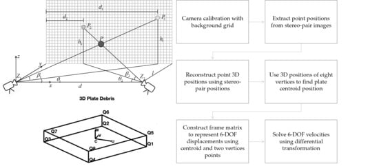
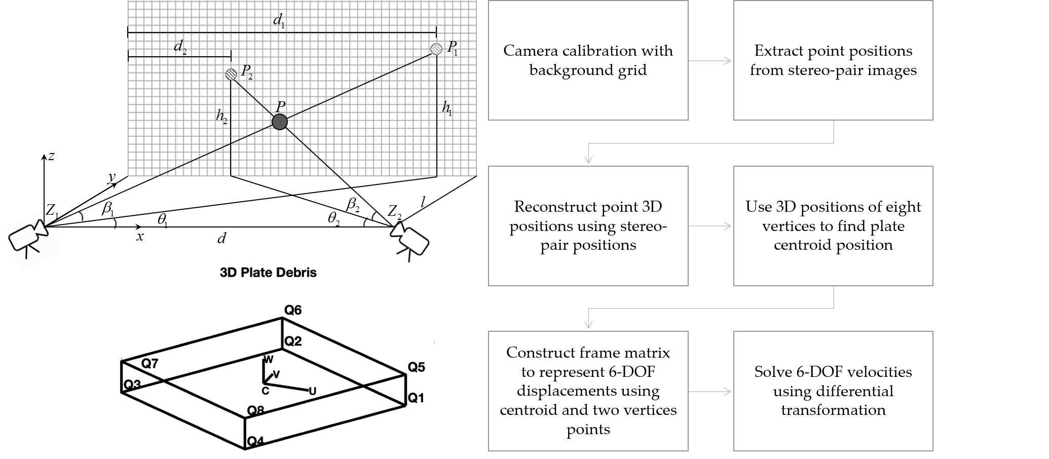
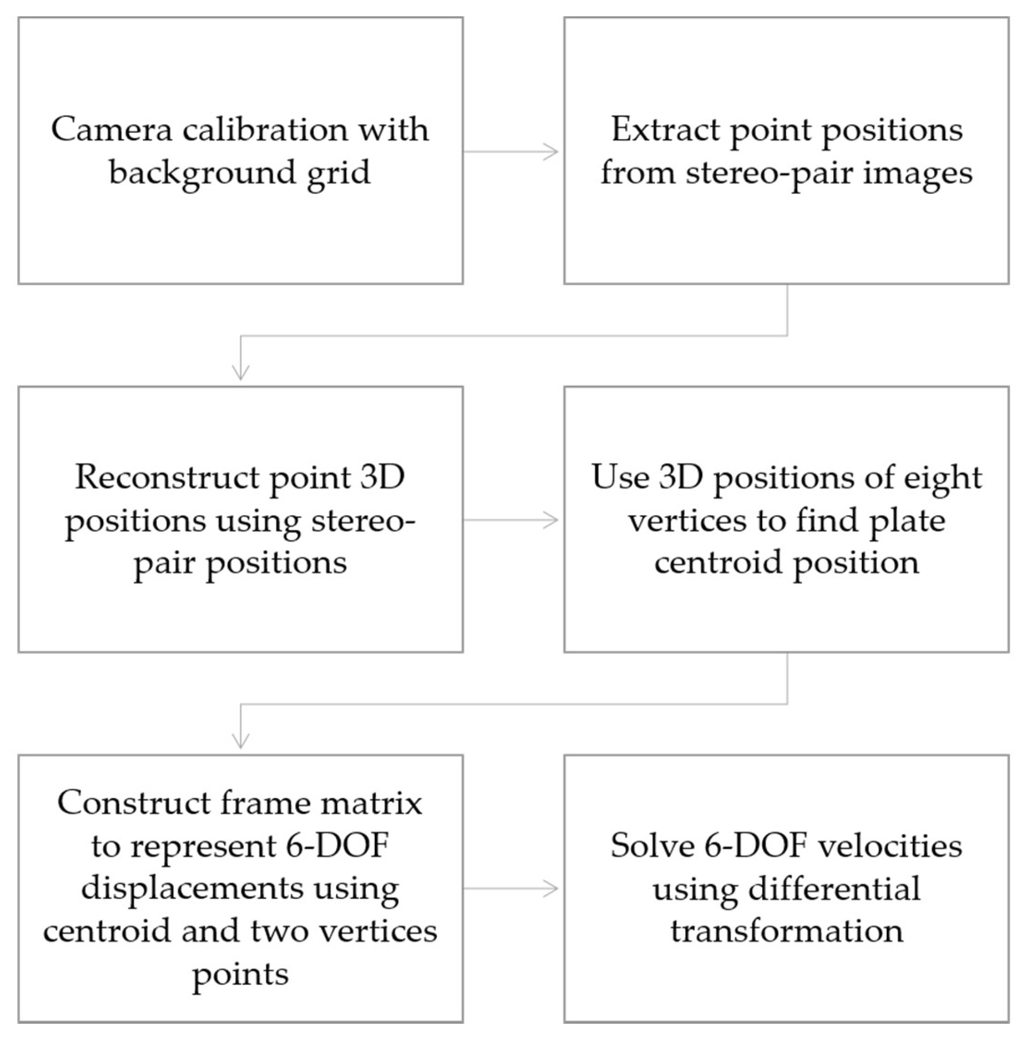
With this we complete the derivation of the formulations for determining the 6-DOF position and orientation along with the 6-DOF translation and rotational velocity of the rigid body debris. The full process of the proposed method for measuring the trajectory of plate-type debris is illustrated in Figure 3.

6. Conclusions

In this paper, we propose an algorithm to reconstruct the 6-DOF (three translational and three rotational) trajectory of flying debris using stereopairs of images from two high-speed cameras. Both the time histories of displacements and velocities can be determined by this algorithm. Specifically, this algorithm addresses the research gap in terms of a lack of algorithms/software for measuring three-rotational-DOF using stereophotogrammetry in the literature, and thus contributes to the new measurement science enabled by high-speed cameras and computer graphics theory. It is intended to be used for experimentally measuring the debris trajectory in a 3D wind field to support the investigation of the debris flight physics in an urban built environment and ultimately contributes to enhancing the reliability of building envelopes under windborne debris hazards. However, it may also be applied to reconstructing the 3D motion of people using surveillance cameras in buildings (e.g., to see how a robber is approaching a victim) or of vehicles in car accidents using traffic monitoring cameras. In this paper, we focused on the wind engineering application and developed this algorithm for two common types of debris, i.e., compact and thin-plate-like, in particular. For the former, the three-translational-DOF were reconstructed. Then the results were used to derive the three-rotational-DOF of the thin plate. In future studies, the algorithm can also be extended for rod-like debris, another type of debris commonly observed during wind risk. The current paper dealt with the theoretical development of the algorithm, while its implementation in conjunction with image processing techniques in wind tunnel experiments will be explored in our future studies.

References

- Holmes, J.D. Windborne debris and damage risk models: A review. Wind Struct. 2010, 13, 95–108. [Google Scholar] [CrossRef]
- Minor, J.E. Lessons learned from failures of the building envelope in windstorms. J. Archit. Eng. 2005, 11, 10–13. [Google Scholar] [CrossRef]
- Lee, B.E.; Wills, J. Vulnerability of fully glazed high-rise buildings in tropical cyclones. J. Archit. Eng. 2002, 8, 42–48. [Google Scholar] [CrossRef]
- Behr, R.A.; Minor, J.E. A survey of glazing system behavior in multi-story buildings during hurricane andrew. Struct. Des. Tall Build. 1994, 3, 143–161. [Google Scholar] [CrossRef]
- Sparks, P.R.; Schiff, S.D.; Reinhold, T.A. Wind damage to envelopes of houses and consequent insurance losses. J. Wind Eng. Ind. Aerodyn. 1994, 53, 145–155. [Google Scholar] [CrossRef]
- Dade County. Building Code Evaluation Task Force Final Report; Dade County: Miami, FL, USA, 1992.
- Dade County. Final Report of the Dade County Grand Jury, Dade County Grand Jury—Spring Term A.D. 1992; Dade County: Miami, FL, USA, 1992.
- Federal Emergency Management Agency. Building Performance: Hurricane Andrew in Florida; Federal Insurance Administration, FEMA: Washington, DC, USA, 1992.
- Wind Engineering Research Council (WERC). Preliminary Observations of WERC Post-Disaster Team; Wind Engineering Research Council (WERC): College Station, TX, USA, 1992. [Google Scholar]
- Oliver, C.; Hanson, C. Failure of residential building envelopes as a result of Hurricane Andrew in Dade County, Florida. In Hurricanes of 1992: Lessons Learned and Implications for the Future; Cook, R.A., Soltani, M., Eds.; ASCE: New York, NY, USA, 1994; pp. 496–508. [Google Scholar]
- Beason, W.L.; Meyers Gerald, E.; James Ray, W. Hurricane related Window glass damage in Houston. J. Struct. Eng. 1984, 110, 2843–2857. [Google Scholar] [CrossRef]
- Tachikawa, M. Trajectories of flat plates in uniform flow with application to wind-generated missiles. J. Wind Eng. Ind. Aerodyn. 1983, 14, 443–453. [Google Scholar] [CrossRef]
- Lin, N.; Letchford, C.; Holmes, J. Investigation of plate-type windborne debris. Part I. Experiments in wind tunnel and full scale. J. Wind Eng. Ind. Aerodyn. 2006, 94, 51–76. [Google Scholar] [CrossRef]
- Lin, N.; Holmes, J.D.; Letchford, C.W. Trajectories of wind-borne debris in horizontal winds and applications to impact testing. J. Struct. Eng. 2007, 133, 274–282. [Google Scholar] [CrossRef]
- Jain, A. Wind borne debris impact generated damage to cladding of high-rise building. In Proceedings of the 12th Americas Conference on Wind Engineering (12ACWE), Seattle, WA, USA, 16–20 June 2013. [Google Scholar]
- Visscher, B.T.; Kopp, G.A. Trajectories of roof sheathing panels under high winds. J. Wind Eng. Ind. Aerodyn. 2007, 95, 697–713. [Google Scholar] [CrossRef]
- Kordi, B.; Kopp, G.A. Effects of initial conditions on the flight of windborne plate debris. J. Wind Eng. Ind. Aerodyn. 2011, 99, 601–614. [Google Scholar] [CrossRef]
- Kordi, B.; Traczuk, G.; Kopp, G.A. Effects of wind direction on the flight trajectories of roof sheathing panels under high winds. Wind Struct. 2010, 13, 145–167. [Google Scholar] [CrossRef]
- Crawford, K. Experimental and Analytical Trajectories of Simplified Debris Models in Tornado Winds. Master’s Thesis, Iowa State University, Ames, IA, USA, 2012. [Google Scholar]
- Hughes, J.F.; Dam, A.V.; McGuire, M.; Sklar, D.F.; Foley, J.D.; Feiner, S.K.; Akler, K. Computer Graphics: Principle and Practice, 3rd ed.; Addison Wesley Professional: Boston, MA, USA, 2013. [Google Scholar]
- Niku, S.B. Introduction to Robotics Analysis, Control, Applications, 2nd ed.; Wiley: Hoboken, NJ, USA, 2011. [Google Scholar]
Figure 1.
The setup of parameters for the trajectory tracking problem (adapted from [19]).
Figure 2.
Rectangular plate representing debris.
Figure 3.
Flowchart of debris-tracking algorithm.
© 2019 by the authors. Licensee MDPI, Basel, Switzerland. This article is an open access article distributed under the terms and conditions of the Creative Commons Attribution (CC BY) license (http://creativecommons.org/licenses/by/4.0/).
Share and Cite
MDPI and ACS Style
Sabharwal, C.L.; Guo, Y. Tracking the 6-DOF Flight Trajectory of Windborne Debris Using Stereophotogrammetry. Infrastructures 2019, 4, 66. https://0-doi-org.brum.beds.ac.uk/10.3390/infrastructures4040066
AMA Style
Sabharwal CL, Guo Y. Tracking the 6-DOF Flight Trajectory of Windborne Debris Using Stereophotogrammetry. Infrastructures. 2019; 4(4):66. https://0-doi-org.brum.beds.ac.uk/10.3390/infrastructures4040066
Chicago/Turabian StyleSabharwal, Chaman Lal, and Yanlin Guo. 2019. "Tracking the 6-DOF Flight Trajectory of Windborne Debris Using Stereophotogrammetry" Infrastructures 4, no. 4: 66. https://0-doi-org.brum.beds.ac.uk/10.3390/infrastructures4040066