Model Calibration Methodology to Assess the Actual Lighting Conditions of a Road Infrastructure

Abstract

Street lighting plays an important role in the comfort and safety of drivers and pedestrians, so the control and management of the lighting systems operation and consumption is an essential service for a city. In this document, a methodology is presented to calibrate lighting models in order to assess the lighting performance through simulation techniques. The objective of this calibration is to identify the maintenance factor of the street lamps, determine the real average luminance coefficient of the road pavement and adapt the reflection properties of the road material. The method is applied in three stages and is based on the use of Radiance and GenOpt software suits for the modeling, simulation, and calibration of lighting scenes. The proposed methodology achieves errors as low as 13% for the calculation of illuminance and luminance, evincing its potential to assess the actual lighting conditions of a road.

1. Introduction

Artificial lighting has a great potential for savings since it accounts for 15% of the electricity consumption of the world and 5% of greenhouse gas emissions [1], with inefficient light sources still being used [2,3]. Ambitious energy policies and strategies for the future have been implemented on the part of the International Energy Agency (IEA) [4] and the European Union (EU). The 2030 climate and energy framework of the EU includes three targets to reduce 40% of greenhouse gas (GHG) emissions since 1990, increase renewable energy share to 32% and improve energy efficiency by at least 32.5% [5]. These energy reduction approaches are aligned with the Lighting Europe’s Strategy Roadmap 2025, focused on enhancing the lighting quality through LEDification, intelligent lighting systems, and human centric lighting based on a circular economy. Many studies have been dedicated to the study of indoor building lighting systems [6,7,8,9,10,11,12] to design energy saving measures. However, one of the main energy consumers is road lighting, representing around 1.3% of the global electricity use [2]. This research is focused on street and road lighting facilities considering that an adequate lighting system is essential for a city and its inhabitants. Artificial lighting contributes to the visibility and recognition of motorists and pedestrians, so it presents a great impact on road safety, well-being, and crime prevention [13,14,15].

Lighting optimization play an important role in the strategies to reduce energy consumption and lighting pollution [16]. For an optimal design of road lighting systems, EN 13201-2:2015 standard [17] provides photometric requirements on roads with motorized traffic (M lighting class), conflict areas (C lighting class) and pedestrians and pedal cyclists streets (P lighting class). Directives to select the most appropriate lighting class are included in technical report TR 13201-1:2014 [18]. Significant energy savings and CO₂ emission reductions can be achieved by also including energy performance indicators in the decision tools used in lighting studies [19] as well as considering traffic intensity data in the design of intelligent outdoor lighting [20]. The implementation of optimization techniques by simulation tools is also useful to improve the safety of the citizens as well as to manage the operation and the costs of the street lighting facilities. The most accepted lighting simulation tools and their combined use have been investigated by Baloch et al. [21], deducing that MATLAB is the most popular software adopted by researchers for lighting simulation and EnergyPlus for energy consumption. MATLAB was used by Shaikh et al. [11] to develop an intelligent multi-objective system for the management of the energy efficiency in buildings and the users’ comfort. However, other tools such as Radiance, Daysim, BuildOpt, DIALux, Relux, or Oxytech have also been used by other authors in their works. Zhang et al. [12] optimized the design of a school building using genetic algorithms and combining thermal and daylight simulations with EnergyPlus and Radiance. Manzan [22] carried out a genetic optimization approach to design the optimal externally shading device using Daysim to compute lighting loads. Yoomak et al. [23] analyzed by means of an optimization and a simulation in Dialux the influence of the pole spacing and the mounting height of the luminaires in the lighting quality comparing high pressure sodium (HPS) and light emitting diode (LED) luminaires. These authors considered different road conditions (wet and dry) and street lamps arrangements (staggered, opposite and single-sided) for their work, concluding that HPS luminaires can provide better average luminance whereas LED luminaires can achieve better visual and comfort performance. Vera et al. [8] implemented the hybrid particle swarm optimization/Hooke–Jeeves (PSO/HJ) algorithm combining a variety of tools for lighting and thermal simulation. They applied an efficient and robust process using Radiance, GenOpt and EnergyPlus.

Modeling outdoor scenes and optimizing their operation requires reflection properties of the road pavement, but the main methods to collect these data consist of laboratory or in-situ measurements [24]. The laboratory measurements demand a small sample of the road surface that must be cut and transported to the laboratory, which makes the process technically and economically complex. For the in-situ measurements, a portable reflectometer must be used. Considering the specific equipment necessary for these methods and their high cost, the most common practice is to adopt the reflection properties of a measured road with similar composition and construction method for which data are available in reflection tables, r-tables. However, the reflection properties mentioned are based on pavement materials measured in 1970s [25,26] and recent studies show that these data are not representative of the asphalt used nowadays [13,22,27]. Many authors have studied the photometric characteristics of existing pavements. Moretti et al. [28] conducted a research that analyzes a variety of pavements in tunnels and states that the whiter the pavement is, the less illuminance is necessary to achieve equal luminance values, reducing power consumption and improving visibility for drivers. Fotios [29] studied new concrete-based pavement materials such as porous asphalt or stone mastic asphalt, concluding that the representative road surface approach cannot describe accurately the reflection characteristics of these new materials. Chen et al. [26] detailed a portable instrument to perform in-situ measurements of the average luminance coefficient (Q₀) of a road in order to scale the standard r-tables with their particular value. Gidlund et al. [30] analyzed the impact on energy saving by comparing between taking into account the standard r-tables or laboratory measurements of a pavement sample in the design conditions of the installation, evidencing that the use of flux control systems are necessary to compensate the data discrepancies. Additionally, new asphalts such as cool pavements are being developed to mitigate the heat island phenomenon and reduce the temperature of cities [31] and due to the use of white high reflective paints they have very different properties from conventional materials. All these studies revealed the need to develop methodologies to characterize new asphalts at reduced costs and obtain new r-tables.

This document proposes a three-phase calibration methodology to obtain more precise models in order to evaluate the performance of outdoor lighting systems in motorized traffic roads. The objective is, on the one hand, to reflect the real deterioration of the luminaires in the model, and, on the other, to improve the modeling of the road surface properties, taking into account the discrepancies between the data used by default and the actual behavior of the pavements and the technical complexity of applying conventional measurement methods. First, a general method that can be applied to different lighting technologies and a variety of road conditions is presented. The approach is based on the combined use of Radiance, to execute the lighting simulations, and GenOpt, for the calibration by means of the Hooke–Jeeves algorithm. Then, this method is applied and validated with a real case study and the results obtained are analyzed and discussed.

2. Materials and Methods

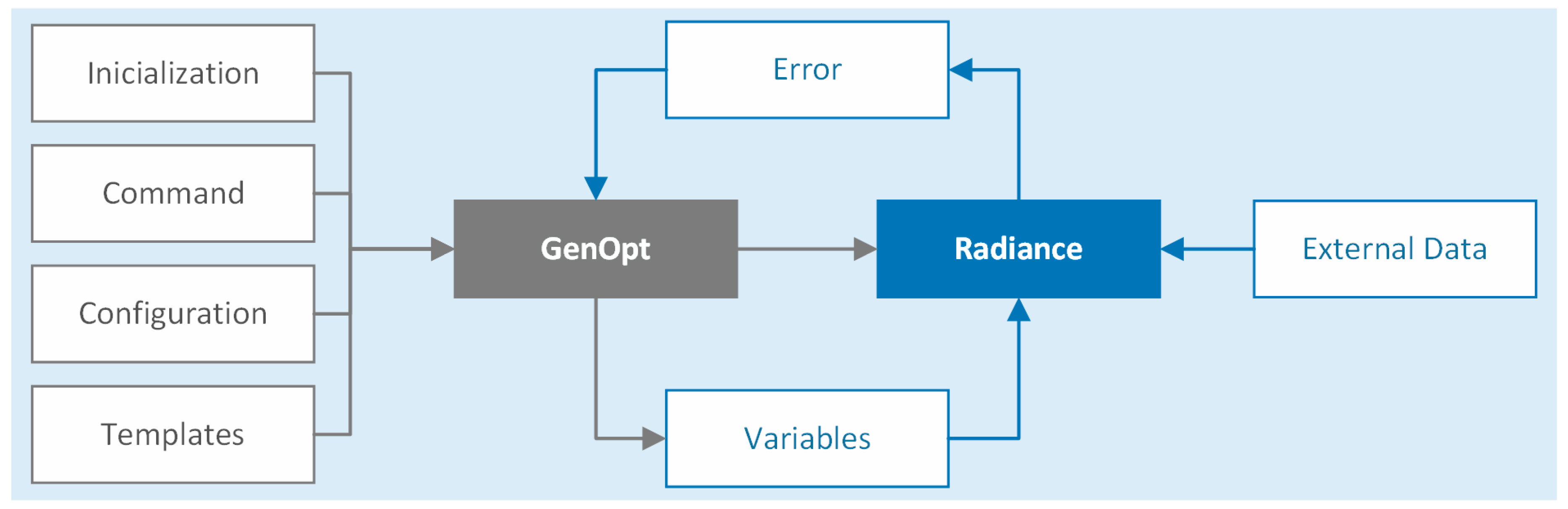
In this work, a deterministic calibration methodology geared to street lighting models is presented. The main purpose is to achieve models that reliably reflect the real conditions of the lighting system and the road so as to evaluate their operation and perform lighting optimization using simulation techniques. The calibration process is carried out using GenOpt as the optimization engine, which is a tool focused on minimizing the value of a certain cost function that is evaluated with other simulation software such as Radiance. Radiance is a suite of tools developed by the Lawrence Berkeley National Laboratory [32] that can be combined to recreate the environmental and lighting conditions of a variety of scenes. As part of the method, Radiance is used to model and simulate external lighting installations implementing the light-backwards ray tracing algorithm. Both tools work together in a custom software pipeline developed in the Python programming language.

GenOpt is used in this work to leverage the Hooke–Jeeves algorithm, which is based on the generalized pattern search (GPS). Its search pattern method [33] generates exploration directions iteratively combining exploratory movements and pattern movements under heuristic rules. The algorithm modifies the calibration parameters between the lower and upper established limits, starting from predefined values. For each iteration, the Radiance programs are executed by GenOpt, as shown in Figure 1, in order to simulate the scene and evaluate the cost function by comparing the model predictions and the measurements collected. The process ends when an optimal result that minimizes the error is achieved.

The coefficient of variation of the root mean squared error (CV(RMSE)) and the root mean squared error (RMSE) are used to evaluate the method [34], which can be calculated through Equations (1) and (2),

$$CV\left(RMSE\right)=\frac{\sqrt{\frac{1}{n}{\sum }_{n=1}^n{\left(\widehat{y_i}-y_i\right)}^2}}{\overline{y}}$$

(1)

$$RMSE=\sqrt{\frac{1}{n}{\displaystyle \sum }_{n=1}^n{\left(\widehat{y_i}-y_i\right)}^2}$$

(2)

where $\widehat{y_i}$ represents the variable measure, $y_i$ indicates the predicted value for this variable, $\overline{y}$ is the arithmetic mean of the measured samples, and $n$ is the number of considered measures. The method stages in which variables with the same units of measure are considered to calculate the error are assessed through the RMSE. Nevertheless, to compare calibrations carried out with different variables, a dimensionless index as the CV(RMSE) is used.

For the error calculation, different lighting evaluation criteria are utilized according to the variables to be calibrated. The purpose of lighting simulations is to design lighting systems that take care of the comfort of drivers and reduce the possibility of accidents at night. For this reason, to assess lighting quality with respect to the lighting level, luminance and illuminance parameters are defined and used in this work. The illuminance describes the amount of light that falls upon the road surface without relation to the lightness of that surface. However, luminance is strongly related to the shine that affects motorists since it denotes the light that is reflected from the road surface and, therefore, its lightness. The luminance of a road surface in any point can be expressed from the illuminance, $E$, through the luminance coefficient, $q$, that represents the reflection characteristics of the road surface as shown in Equation (3).

$$L=q·E$$

(3)

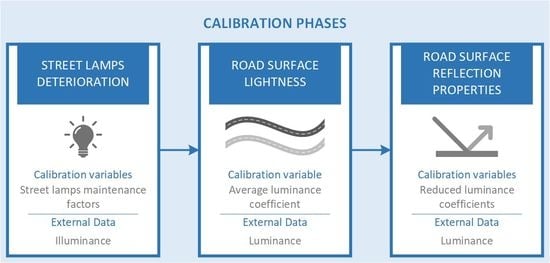
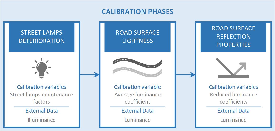
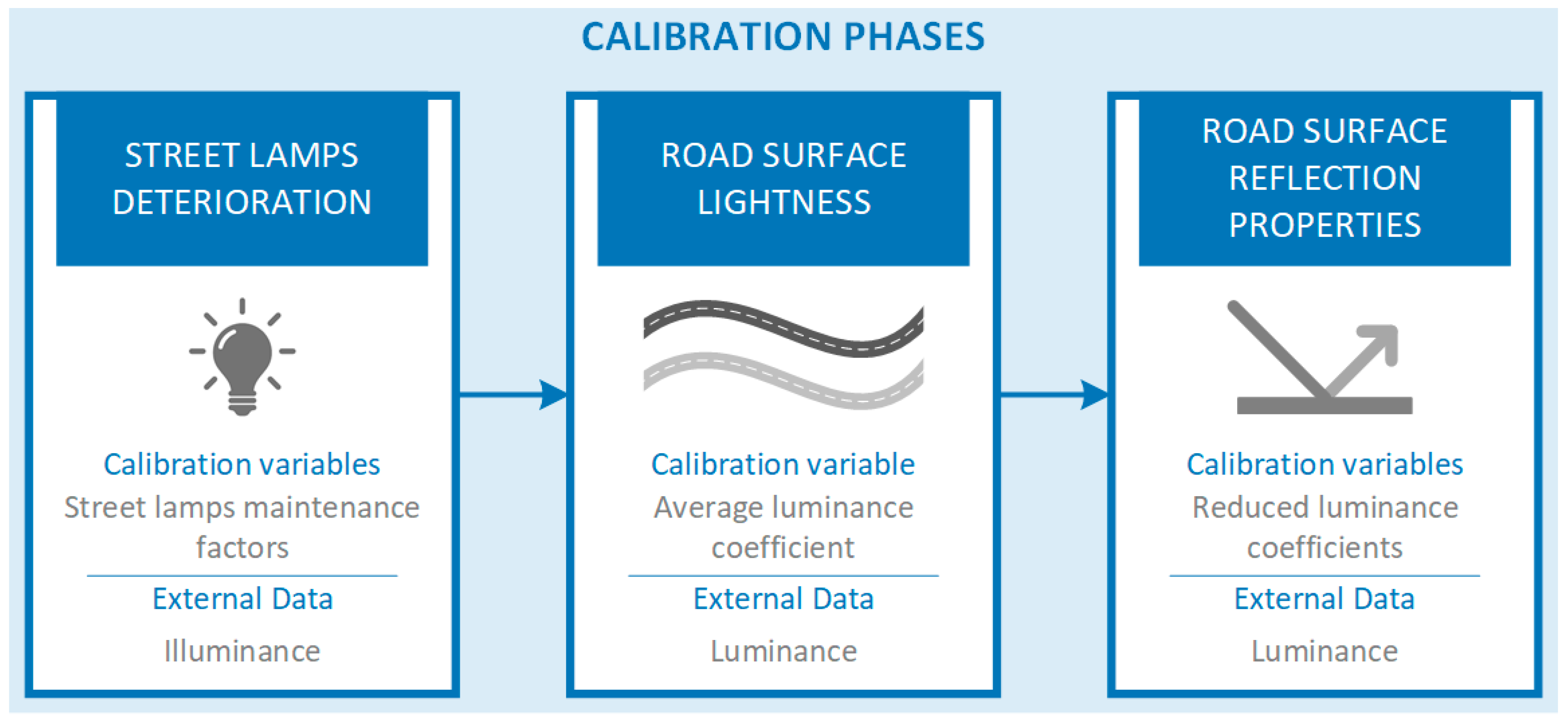
The calibration is carried out in three stages, indicated in Figure 2, trying to reduce the error successively: (i) maintenance factor identification of each luminaire, that allows for the calibration of the model from the illuminance of the scene by adjusting the amount of light emitted by the luminaries; (ii) calibration of Q₀ parameter, related to the type of pavement considered in the modeling stage, according to the luminance of the road; and (iii) adaptation of the reflection properties of said asphalt also using experimental luminance data.

2.1. Maintenance Factor Identification

This stage of the method allows for the identification of the individual maintenance factor [35,36] of each luminaire of the lighting installation, related to the lumen depreciation of the lamps, the dirt of lamps and luminaires and the probability of not failing in a specific time. This process is used to generate a model where the deterioration of the road lighting system is taken into account. For this, in order to improve the model and reduce errors made during the modeling and data collection stages, the calibration methodology presented in previous works of the authors is applied [37].

The design value used for the maintenance factor is calculated specifically for the lamps of the experimental system in accordance with CIE 154:2003 [35] and ISO/CIE TS 22012:2019 [36]. For the calibration, the error is calculated comparing the illuminance measured experimentally on the road and the illuminance estimated for the simulation software in a set of points.

2.2. Average Luminance Coefficient Calibration

The second stage of the method aims to improve the lighting model by correcting some of the inaccuracies derived from the modeling of the road material. For this purpose, the Q zero-S1 description system established by the CIE 030.2:1982 [38] is adopted. This system considers that most of the pavements can be described by means of their lightness and their specularity using the average luminance coefficient, Q₀, and the specular factor, S1, respectively. It should be noted that higher values of Q₀ correspond to darker surfaces, whereas a low S1 value represents a more diffuse and less specular surface.

The CIE 144:2001 [25] establishes different classifications of dry road surfaces (

Table 1. R-classification system for dry road surfaces established by the CIE.

Class	S1 Limit	Table	S1 Standard	Q0 Standard
RI	S1 < 0.42	R1	0.25	0.10
RII	0.42 ≤ S1 < 0.85	R2	0.58	0.07
RIII	0.85 ≤ S1 <1.35	R3	1.11	0.07
RIV	1.35 ≤ S1	R4	1.55	0.08

) so that a standard can be adopted instead of taking measurements on the road. The most used is the R-classification system, which considers four classes of surfaces, RI-RIV, characterized by its degree of specularity. Each class is associated with a predefined reflection table as well as values of Q₀ and S1, but the table can be rescaled if the real Q₀ of the considered road is known.

Q₀ is calibrated to adapt the lightness of the road, as its real value may be far from the default due to the deterioration of the pavement or simply for design reasons. Moreover, the four types of surfaces of the R-classification are studied, bearing in mind that it is difficult to reliably determine the properties of a given asphalt after deterioration. For all four cases, the calibration methodology is applied considering the standard Q₀ as the design value for the process and the luminance as the variable used for the error calculation. As a result of the method, the Q₀ that reduces the model errors for each kind of surface is obtained. Then, according to the CV(RMSE) and RMSE, it is possible to evaluate and decide which type of surface is more representative and, therefore, better fits the analyzed surface.

2.3. Adaptation of the Closest r-Table

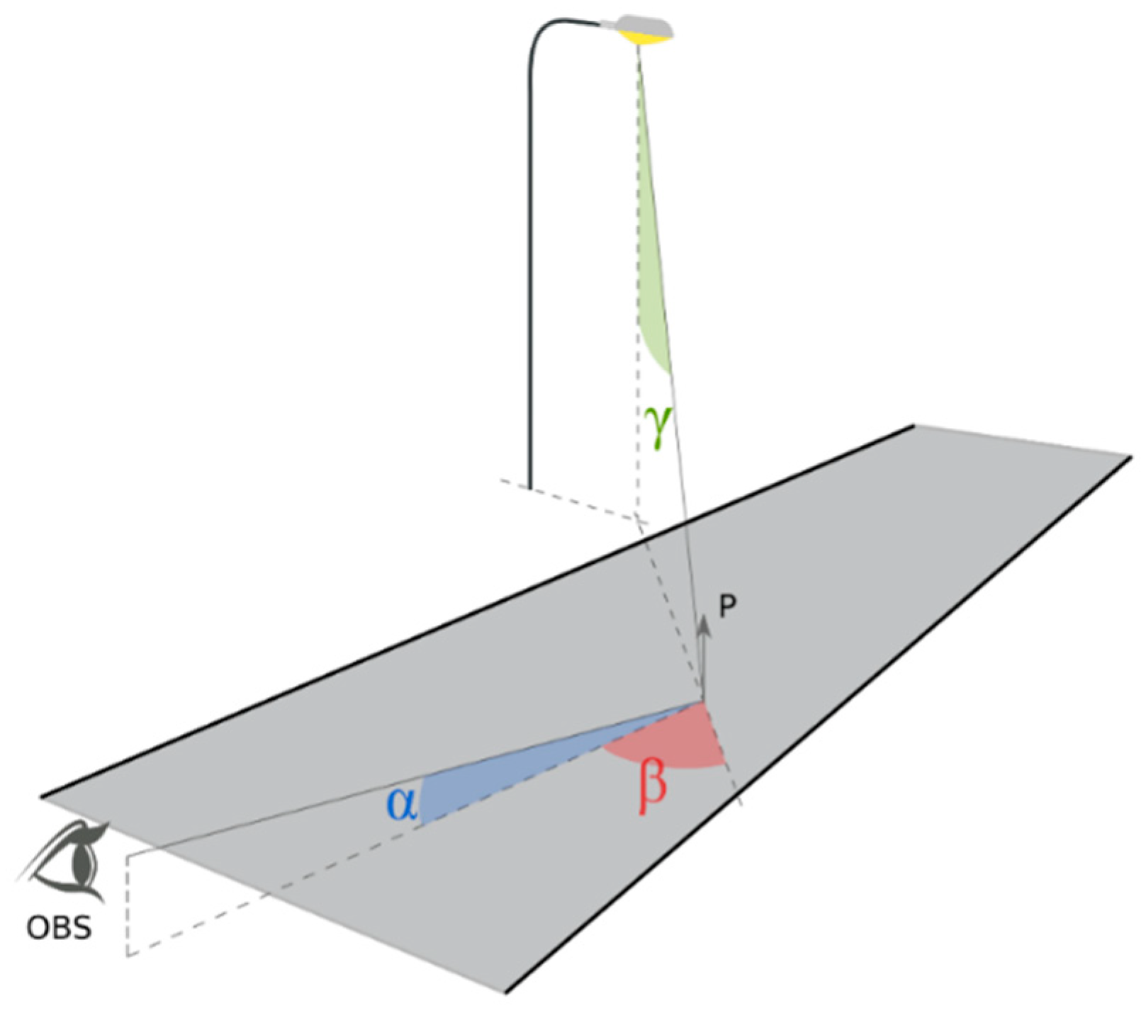
After the road lightness is calibrated, additional improvements in the modeling of the material are introduced in this stage to predict the luminance values with greater precision. The objective is to correctly define the reflection properties of the asphalt modifying the luminance coefficient of each point of the road. The luminance coefficient depends on the attributes of the road material, the observer position, the location of the point that the observer is visualizing, and the incident light direction at that point. Therefore, this parameter can be defined by means of three angles detailed in Figure 3: the observation angle (α), the angle between plane of light incidence and plane of observation (β), and the angle of light incidence (γ). For motorized traffic, α is usually ignored, since it presents little variation for the zone that the driver visualizes and it is typically considered as a constant value [39]. However, this is a general method that can be applied to adapt the reflection properties of the road for different observations angles.

The reflection table, r-table, includes the reflection characteristics of a road surface in terms of reduced luminance coefficients ($r$), related to the luminance coefficients through Equation (4):

$$q=\frac{r\left(\mathsf{\beta },\mathsf{\gamma }\right)}{co{s}^3\mathsf{\gamma }}$$

(4)

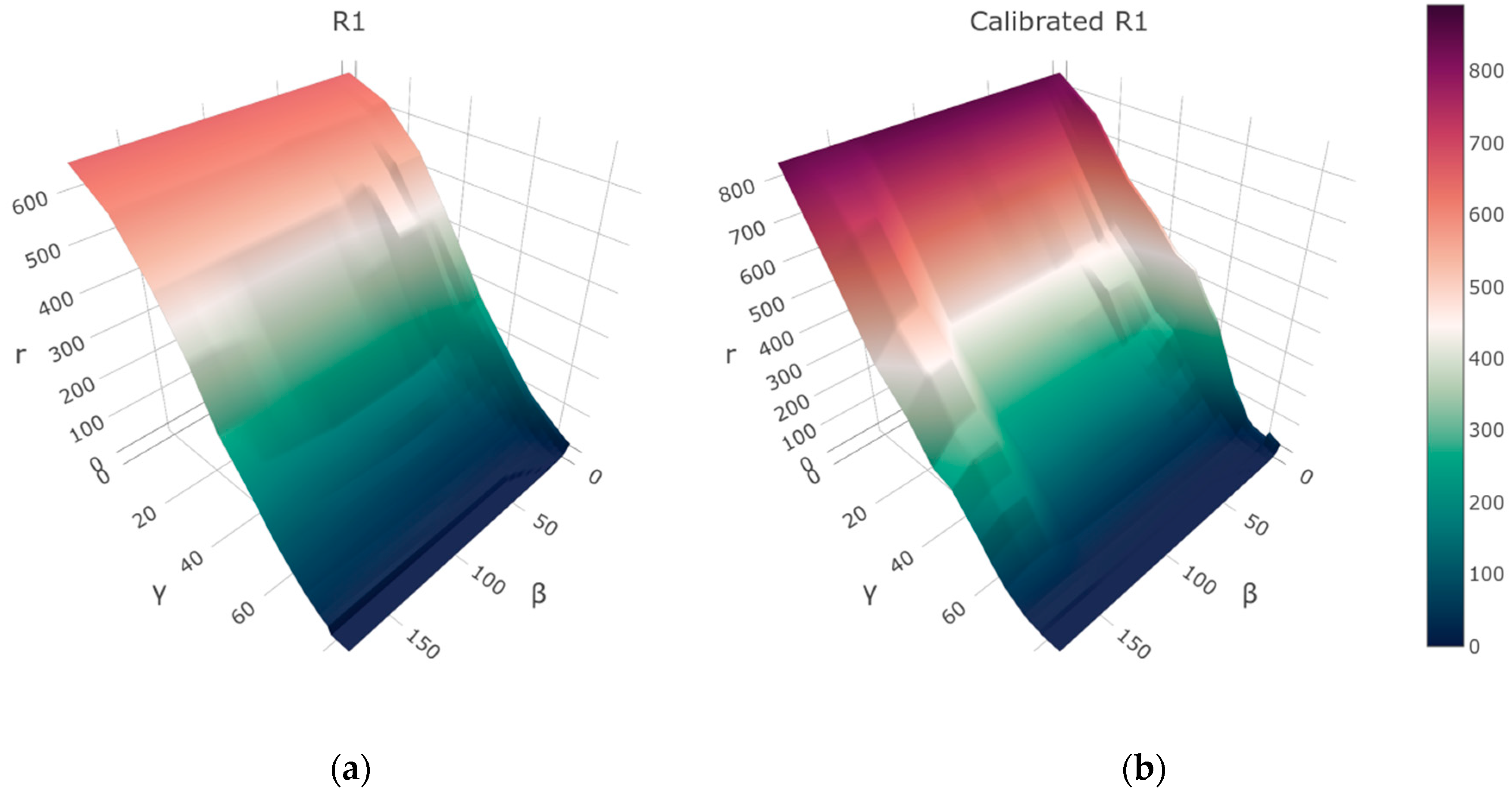
These parameters are specified for 396 combinations of the angles β and γ. The standard r-tables are designed specifically for a constant value of 1° for α, but the main purpose of this work is to develop a general methodology that can be implemented at different observation angles. For this reason, the original r-tables should be adapted to be used in simulations in which the position of the observer does not always correspond to the observation angle that the CIE establishes by default. The contents of the tables also indicate how diffuse or specular the material they represent is. Therefore, it is also interesting to adapt these contents to show the real specularity of the asphalt and not an approximation.

The r-table involves reduced luminance coefficients for the combination of 20 β angles and 29 γ angles. The calibration methodology proposed for the r-table consists on weighting each r coefficient using two multiplying factors, one of them related to the corresponding γ angle and another to the β. In this way, 49 calibration variables intervene in the process, one for each angle of the table. The calibrated r coefficient is calculated using Equation (5),

$$r_{cal}\left(\mathsf{\beta },\mathsf{\gamma }\right)=r\left(\mathsf{\beta },\mathsf{\gamma }\right)·a\left(\mathsf{\gamma }\right)·\left(b\left(\mathsf{\beta }\right)·\tan \mathsf{\gamma }+1\right)$$

(5)

where $a\left(\mathsf{\gamma }\right)$ is the factor corresponding to γ angle, $b\left(\mathsf{\beta }\right)$ represents the factor relative to the β angle and $r\left(\mathsf{\beta },\mathsf{\gamma }\right)$ indicates the reduced luminance coefficient included in the standard r-table.

This approach tries to avoid large variations to preserve a smooth shape. Taking into account the relation between the r-tables and the luminance, this is the factor used to evaluate the optimal result during the calibration. The design value for the calibration variables are those that maintain the original r-table without modifications.

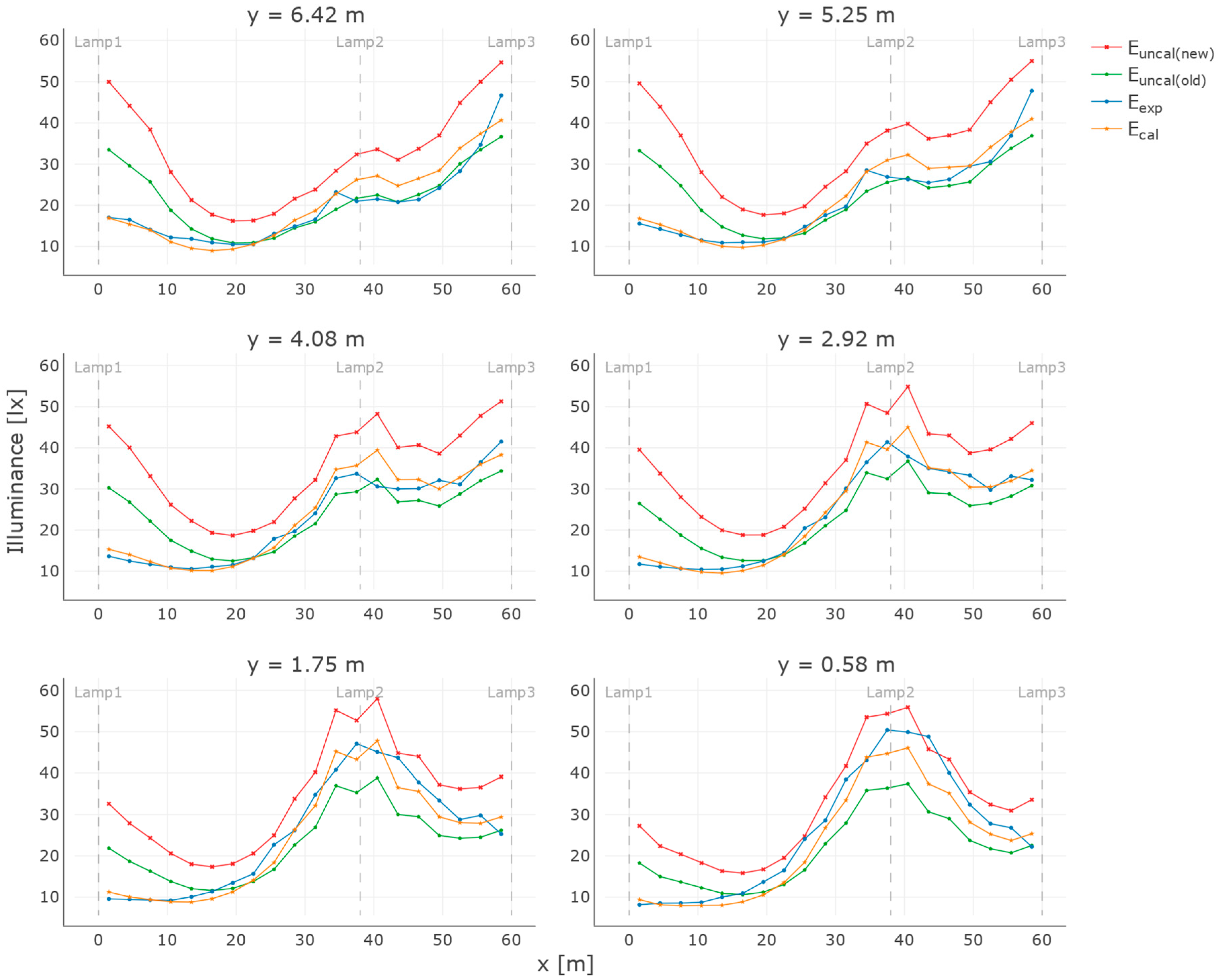
3. Experimental System

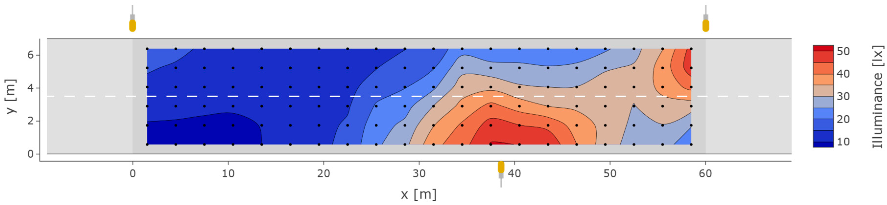
To test the developed methodology, it was applied to a real scenario, comparing real data collected on the road and simulation results. The test scenario is a strech of road located in Nigrán, south of Galicia, Spain. As stablishes in the European Standard EN 13201-3:2015 [39], an area between two lampposts placed on the same side of the road is used for calculations. The considered area is a two-lane road of 60 m length and 7 m width and the lighting installation includes three streetlights organized in staggered arrangement. Each streetlight involves a 250 W HPS light source mounted on a top of a 10 m pole with an overhang of 2 m. On both sides of the road the light points are located 1 m away from the edge.

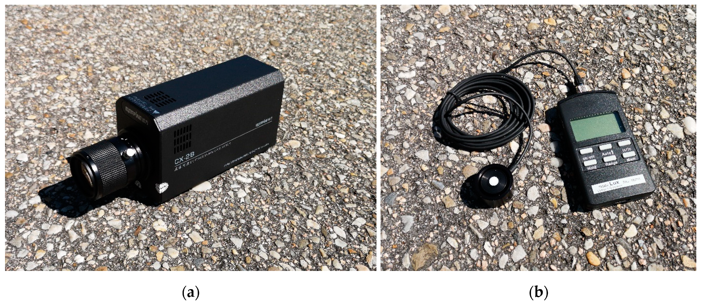
The calibration process described in the methodology demands experimental data about luminance and illuminance, so it was necessary to apply different data collection procedures using the specific measurement equipment showed in Figure 4. The technical specifications of both devices are detailed in

Table 2. Technical features of the Mobilux luxmeter and the CX-2B imaging luminance meter.

Mobilux Luxmeter
Light intensity range	From 0 to 120 klx
Light sensor	Silicon photo diode with V(λ) filter
Light sensitive surface of the diffuser	8 mm
Measuring rate	2 measurements per second
CX-2B Imaging Luminance Meter
Resolution	1360 × 1024
Focal length	56 mm
Luminance accuracy	±5%
CCD working temperature	5 °C
Field of view	9.1° (horizontal) × 6.7° (vertical)

. Illuminance on the road was collected using a portable luxmeter from Czibula & Grundmann GmbH, taking measurements at evenly distributed points on the road. According to the standard EN 13201-3:2015 [39], a grid of points with 6 rows and 20 columns is considered, so that points are spaced at regular intervals of 3 m in the x axis and 1.167 m in the y axis. The maintenance factor specifically calculated for this case was 0.67, a typical value for a low-maintenance installation that includes HPS lamps with long hours of operation and IP6x luminaires in a polluted environment [35]. All these data are used for the identification of the maintenance factors of the luminaires in the calibration process. 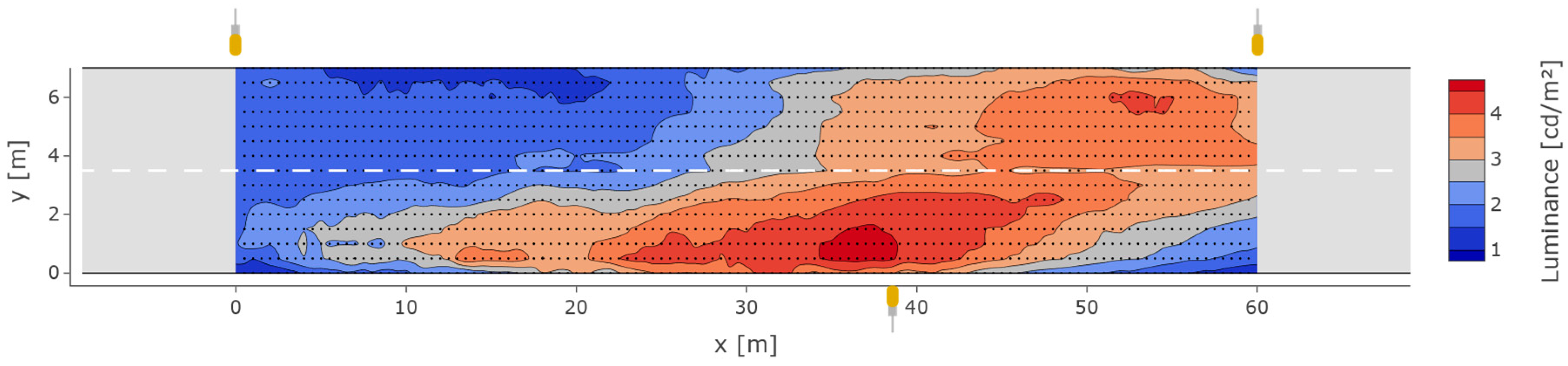Figure 5 shows the positions of the measured points, the illuminance in those points and the distribution of the street lamps on the roadway.

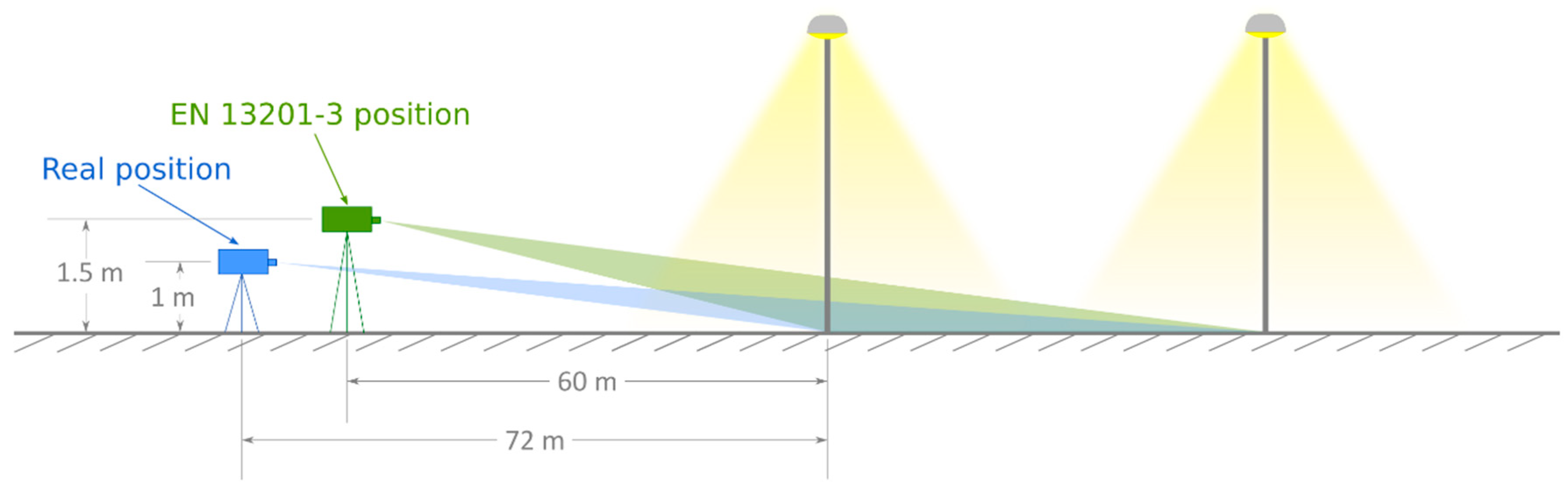
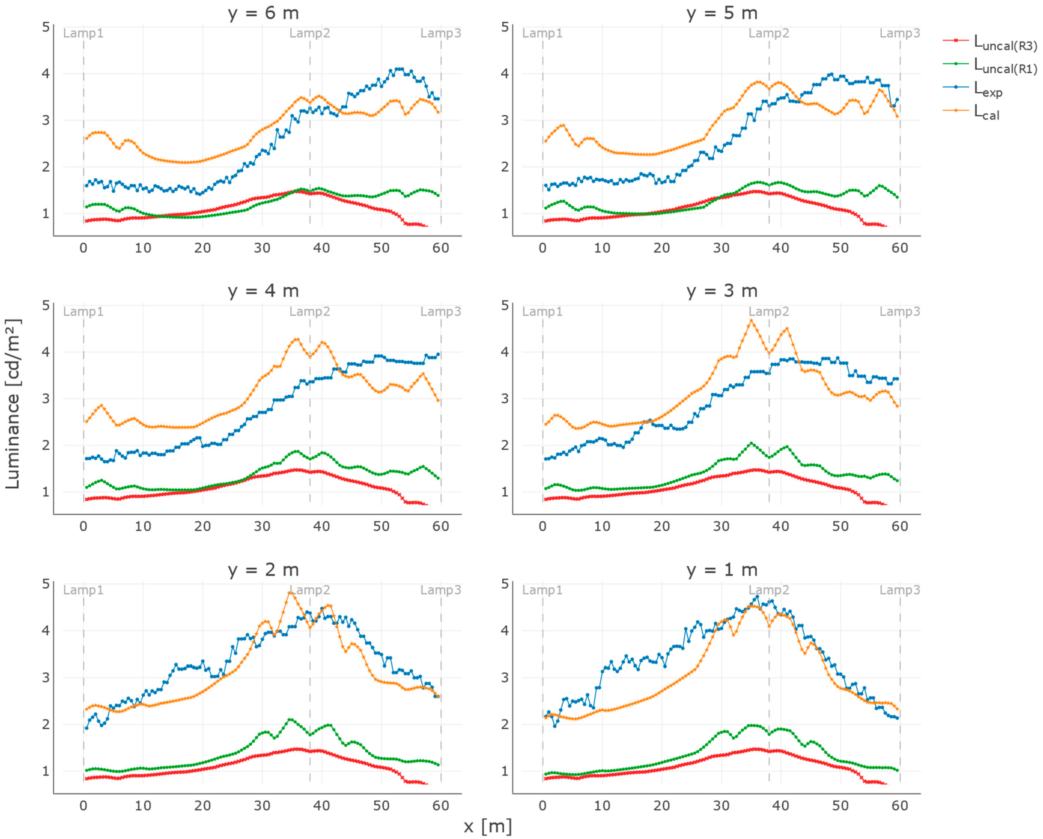
Furthermore, in order to collect luminance data from the road, a charge coupled device (CCD) luminance meter was used, a CX-2B model from Everfine Corporation. The luminance meter was approximately located on the central line of separation between the two lanes, spaced 72 m from the beginning of the calculation area and 1 m from the ground. Figure 6 shows the difference with respect to the data acquisition procedure proposed by EN 13201-3:2015 [39], in which the recommendation is to position the luminance meter in the center of each lane at a separation of 60 m with respect to the calculation area and 1 m in height. An observer position different than EN 13201-3 is chosen in order to generalize the methodology and demonstrate that it is valid for different observations angles. This is interesting since there is an increasingly common trend of obtaining measurements in a more automated way such as installing the measurement devices in vehicles in which it is sometimes complicated to ensure the exact position.

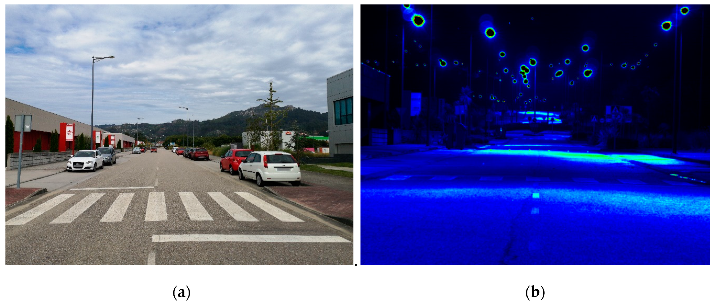
In order to avoid errors introduced during the measurement process, the PnP (Perspective-n-Point) method was used to accurately determine and validate the position of the equipment based on several control points placed on the street. The discrepancies between both measurement systems for the location of the luminance meter can be checked in

Table 3. Discrepancies between measuring the position of the luminance meter manually or using the PnP method.

Variable	Measured Value	PnP Value
x	72.000	72.002
y	3.500	3.568
z	1.000	1.083

. The PnP problem was solved through an iterative method based on the Levenberg–Marquardt optimization [40,41]. The equipment was oriented towards the calculation field, simulating the position of the observer. The result is a perspective image, as shown in Figure 7, where the luminance in the area can be appreciated.

The calculation area is selected in the perspective luminance image and the pixel values enclosed in that region are used to calculate the luminance values in the corresponding road plane. The correspondence between 2D and 3D points was made considering the intrinsic parameters and the distortion coefficients of the calibrated CCD sensor. The camera was calibrated using a set of 27 chessboard images and following the algorithm based on the work of Zhang [42] and Bouguet [43]. The average reprojection error obtained from the calibration process is 0.502 px. 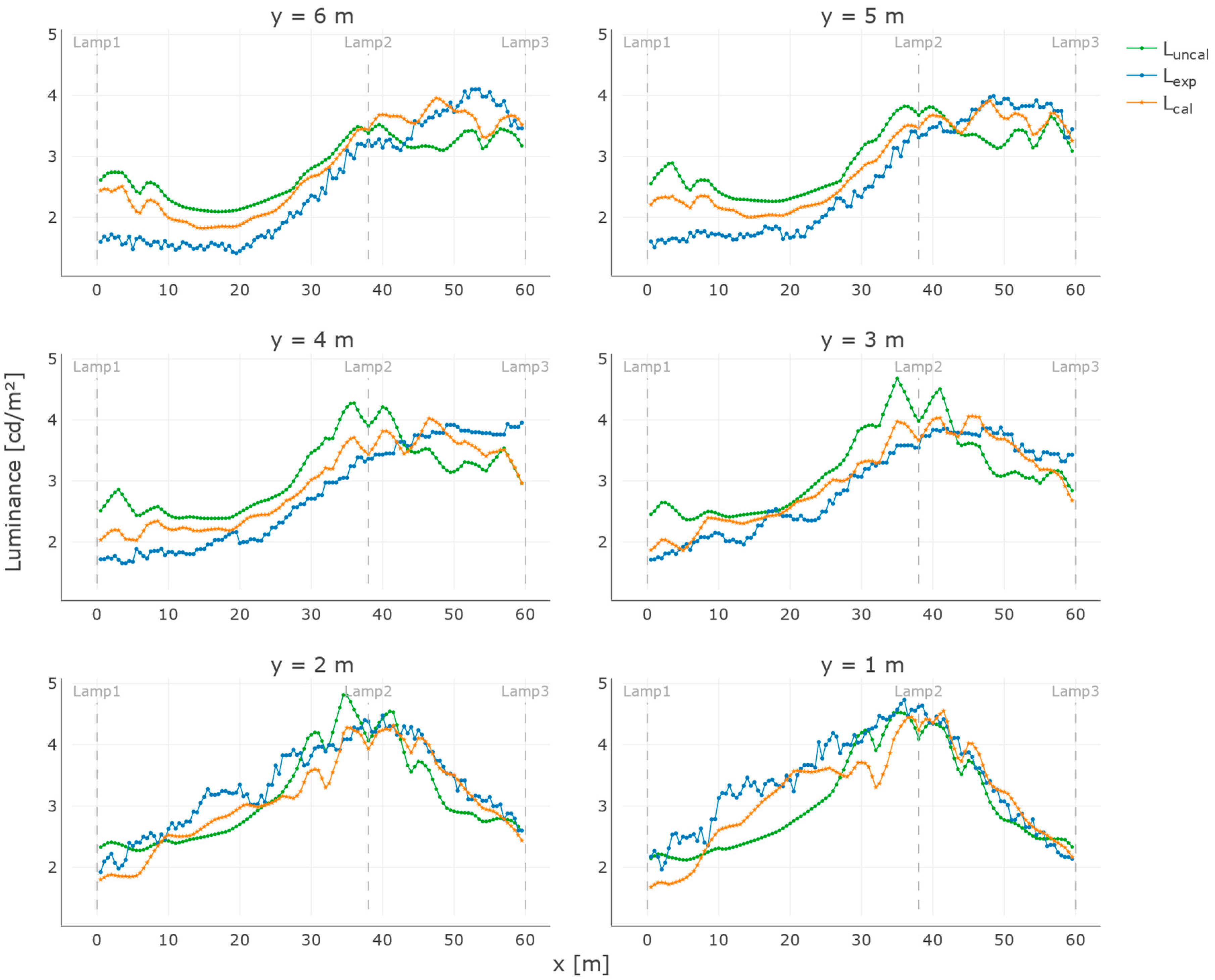Figure 8 illustrates a matrix in which each pixel is associated to the luminance of the corresponding road section after the perspective transformation. From this image, luminance data of points spaced at regular intervals of 0.5 m in x and y axis are picked to calibrate the model in the last two stages: the calibration of the Q₀ factor and the adaptation of the r-table.

4. Results and Discussion

In the following sections, the individual results of each of the calibration stages applied to the case study are analyzed.

4.1. Maintenance Factor Identification

To graphically analyze the results, longitudinal sections of the road are shown in Figure 9. For each section, experimental illuminance, $E_{exp}$, and simulated illuminance after the calibration of the model, $E_{cal}$, are compared. The similarity between both curves indicates that the method is favorable to reduce the errors of the model and to improve the accuracy of the simulation. The figure also includes a comparison between the experimental illuminance and the simulated illuminance from the uncalibrated model under the following assumptions: (i) the lamps have been installed recently and their maintenance factor is 1 for all of them, $E_{uncal\left(new\right)}$; and (ii) all the lamps have suffered some deterioration, with a typical maintenance factor of 0.67 as explained above, $E_{uncal\left(old\right)}$. Results indicate that each of the luminaries shows different performance. Although the lamps have been installed at the same time and the installation is not recent, it would not be correct to assume a uniform maintenance factor of 0.67 for the entire facility. Two of the lamps show a slightly higher level of illuminance while the other one offers a lower level.

This stage of the method is also used to identify shortcomings in the installation. Lamp maintenance factors calculated with the calibration methodology are included in

Table 4. Calibration variables of the model.

Variable	Design Value	Calibrated Value
Maintenance Factor for Lamp 1	0.67	0.3201
Maintenance Factor for Lamp 2	0.67	0.8481
Maintenance Factor for Lamp 3	0.67	0.7307

. Results show that lamp 1 is the most deteriorated lamp. The wide gap with respect to the others indicates that the lamp probably presents some technical issues. Nevertheless, lamps 2 and 3 show a better operation with a maintenance factor higher than expected. These results are consistent with the visual inspection carried out during the measurement process, in which a malfunction was observed in one of the luminaires.

Table 5. Error estimation for the simulation of the uncalibrated and the calibrated model.

Statistical Error	Initial Simulation	Calibrated Simulation	Reduction (%)
CV(RMSE) (%)	29.73	13.11	55.90
RMSE [lx]	6.88	3.02	56.10

includes the errors calculated from the simulations carried out considering the design value and the calibrated value for the maintenance factor. In terms of illuminance, the error is lowered from 6.88 lx to 3.02 lux, reducing the RMSE by 56%.

4.2. Average Luminance Coefficient Calibration

Results of calibrating the model considering the four pavement classes of the R-classification are included in

Table 6. Results of the calibration of the reduced luminance coefficient for the four pavement classes of the R-classification.

r-Table	Design Value	Calibrated Value	Statistical Error	Initial Simulation	Calibrated Simulation	Reduction (%)
R1	0.10	0.2288	CV(RMSE) (%)	130.96	19.06	85.45
R1	0.10	0.2288	RMSE (cd/m2)	1.73	0.58	66.47
R2	0.07	0.2048	CV(RMSE) (%)	191.52	25.73	86.57
R2	0.07	0.2048	RMSE (cd/m2)	2.02	0.79	60.89
R3	0.07	0.2018	CV(RMSE) (%)	185.30	39.41	78.73
R3	0.07	0.2018	RMSE (cd/m2)	2.03	1.25	38.42
R4	0.08	0.2122	CV(RMSE) (%)	162.32	47.88	70.50
R4	0.08	0.2122	RMSE (cd/m2)	1.98	1.55	21.72

. The calibrated Q₀ is greater than the design value for all the alternatives taken into consideration. This suggests that the road surface studied is less dark than the standard asphalt models adopted. Moreover, if the CV(RMSE) and the RMSE of the four tests are compared, it is verified that the R1 type of asphalt is the one that represents the measured surface with greater precision. Both the CV(RMSE) and the RMSE are lower for this alternative than for the rest, so it will be used to model the road in the following steps of the method. The fact that the surface approaches a type R1 pavement implies that the road is mainly diffuse. The table also shows that with this stage of the method it is possible to reduce the RMSE by 66%.

The main advantage of calibrating the Q₀ factor can be seen in Figure 10, in which the luminance levels in different longitudinal sections of the road have been represented. The luminance before the calibration, $L_{uncal\left(R1\right)}$, and the experimental luminance, $L_{exp}$, can be compared in the image. The data indicate that the simulation of the uncalibrated model is not an accurate method to determine the luminance on the road since the experimental luminance levels are much higher than those simulated. As mentioned, this is due to the fact that the road is not as dark as the standard parameters establish. By increasing the Q₀ factor the results of the calibrated simulation, $L_{cal}$, are closer to the experimental ones. Figure 10 also depicts the luminance calculated using reflection properties of R3 class, $L_{uncal\left(R3\right)}$, the typically pavement class used in lighting design.

4.3. Adaptation of the Closest r-Table

The values adopted by the calibration variables after applying the third stage of the developed methodology are presented in

Table 7. Calibration variables related with the initial and the calibrated model.

Variable	Design Value	Calibrated Value	Variable	Design Value	Calibrated Value
$a\left(\mathsf{\gamma }=0.00\right)$	1.000	1.286	$b\left(\mathsf{\beta }=0\right)$	1	1.188
$a\left(\mathsf{\gamma }=14.04\right)$	0.800	0.947	$b\left(\mathsf{\beta }=2\right)$	1	1.188
$a\left(\mathsf{\gamma }=26.57\right)$	0.667	0.717	$b\left(\mathsf{\beta }=5\right)$	1	0.937
$a\left(\mathsf{\gamma }=36.87\right)$	0.571	0.663	$b\left(\mathsf{\beta }=10\right)$	1	0.607
$a\left(\mathsf{\gamma }=45.00\right)$	0.500	0.618	$b\left(\mathsf{\beta }=15\right)$	1	0.506
$a\left(\mathsf{\gamma }=51.34\right)$	0.444	0.655	$b\left(\mathsf{\beta }=20\right)$	1	0.500
$a\left(\mathsf{\gamma }=56.31\right)$	0.400	0.582	$b\left(\mathsf{\beta }=25\right)$	1	0.500
$a\left(\mathsf{\gamma }=60.26\right)$	0.364	0.541	$b\left(\mathsf{\beta }=30\right)$	1	0.500
$a\left(\mathsf{\gamma }=63.43\right)$	0.333	0.448	$b\left(\mathsf{\beta }=35\right)$	1	0.500
$a\left(\mathsf{\gamma }=68.20\right)$	0.286	0.294	$b\left(\mathsf{\beta }=40\right)$	1	0.500
$a\left(\mathsf{\gamma }=71.57\right)$	0.250	0.228	$b\left(\mathsf{\beta }=45\right)$	1	0.500
$a\left(\mathsf{\gamma }=74.05\right)$	0.222	0.137	$b\left(\mathsf{\beta }=60\right)$	1	0.500
$a\left(\mathsf{\gamma }=75.96\right)$	0.200	0.100	$b\left(\mathsf{\beta }=75\right)$	1	0.500
$a\left(\mathsf{\gamma }=77.47\right)$	0.182	0.091	$b\left(\mathsf{\beta }=90\right)$	1	0.500
$a\left(\mathsf{\gamma }=78.69\right)$	0.167	0.083	$b\left(\mathsf{\beta }=105\right)$	1	0.500
$a\left(\mathsf{\gamma }=79.70\right)$	0.154	0.077	$b\left(\mathsf{\beta }=120\right)$	1	0.500
$a\left(\mathsf{\gamma }=80.54\right)$	0.143	0.072	$b\left(\mathsf{\beta }=135\right)$	1	0.500
$a\left(\mathsf{\gamma }=81.25\right)$	0.133	0.133	$b\left(\mathsf{\beta }=150\right)$	1	1.029
$a\left(\mathsf{\gamma }=81.87\right)$	0.125	0.125	$b\left(\mathsf{\beta }=165\right)$	1	0.890
$a\left(\mathsf{\gamma }=82.41\right)$	0.118	0.118	$b\left(\mathsf{\beta }=180\right)$	1	0.500
$a\left(\mathsf{\gamma }=82.87\right)$	0.111	0.111
$a\left(\mathsf{\gamma }=83.29\right)$	0.105	0.105
$a\left(\mathsf{\gamma }=83.66\right)$	0.100	0.100
$a\left(\mathsf{\gamma }=83.99\right)$	0.095	0.095
$a\left(\mathsf{\gamma }=84.29\right)$	0.091	0.091
$a\left(\mathsf{\gamma }=84.56\right)$	0.087	0.087
$a\left(\mathsf{\gamma }=84.81\right)$	0.083	0.083
$a\left(\mathsf{\gamma }=85.03\right)$	0.080	0.080
$a\left(\mathsf{\gamma }=85.24\right)$	0.077	0.077

. The comparison of these results with the design values initially assigned shows that the method does not introduce large variations in the reduced luminance coefficients, but that it slightly adapts the contents of the r-table in areas where the reflection properties of the asphalt are not correctly represented. Moreover, Figure 11 depicts the standard r-table for the R1 road surface together with the calibrated r-table calculated from the previous variables.

As expected, adapting the r-table has direct effects on the luminance. Figure 12 show the luminance in a set of points in longitudinal sections of the road to establish a comparative relation among the experimental values, $L_{exp}$, and results of the initial simulation, $L_{uncal}$, and the calibrated one, $L_{cal}$. It is observed that after calibration, the luminance values predicted with the simulation are closer to the experimental data collected on the road. This implies that the method is adequate to reduce modeling errors.

The application of the method brings about a reduction of the error by 35% in terms of luminance since the error decreases from 0.57 cd/m² to 0.37 cd/m². Furthermore,

Table 8. CV(RMSE) and RMSE calculated for the initial simulation and the simulation of the calibrated model.

Statistical Error	Initial Simulation	Calibrated Simulation	Reduction (%)
CV(RMSE) (%)	19.06	12.57	34.05
RMSE (cd/m2)	0.57	0.37	35.09

also shows that the CV(RMSE) is reduced by 34%, achieving a value lower than 13% for the calibrated simulation.

5. Conclusions

This document presents a methodology that combines the use of Radiance and GenOpt to simulate and calibrate outdoor lighting models. The method was tested through their application in three phases to a real scenario: first, the luminance factor of each luminaire was identified; then, the real average luminance coefficient of the road material was estimated; and finally, the reflection properties of the asphalt were adjusted. The purpose is to assess the effects of asphalt and luminaires deterioration on simulation results, especially on luminance. Asphalt tends to lighten over the years, increasing the luminance value, while luminaires are susceptible to reduce their luminous flux, contributing to lower luminance values. Thus, considering these two factors separately is especially important to correctly model the entire installation and predict its performance, as their potentially opposite effects might hide the actual behavior of its individual elements.

The identification of the maintenance factor of the street lamps from illuminance data provide a model that includes the actual deterioration suffered over time in the group formed by luminaire and lamp. The 56% reduction of the CV(RMSE) indicates that a considerable error is committed by not taking into account a real estimation of these factors, but that it is feasible to attenuate it after the calibration. This part of the method can be used to distinguish street lamps with operational deficiencies as a method of predictive maintenance and facilitate the management of the installation.

In the second part of the methodology, the Q₀ factor is calibrated in order to evaluate the lightness of the road asphalt using experimental luminance data. This is useful to improve the model by reducing the errors induced by not considering the deterioration of the road. Taking into account that the state of the road is not the same throughout its useful life, it is interesting to re-evaluate the properties of the asphalt every so often, especially before addressing modifications in the lighting system. Results corroborate that it is possible to achieve a CV(RMSE) reduction of 86% for the case study.

The r-table is adapted to reflect the real degree of specularity of the road material in the last step. This allows for the correction of the standard r-tables specified by the CIE from collected luminance data. The aim is to reproduce the real reflection properties of the road to consider them in the simulations and obtain more reliable results. The implementation of this part of the method supposes a decrease of 34% for the CV(RMSE) with respect to the non-calibrated simulation.

Overall, this work shows that this research can contribute to the improvement of modeling and simulation methods as well as the street lighting maintenance and the assessment of real road conditions.

References

1. United Nations Environment Programme. Accelerating the Global Adoption of Energy-Efficient Lighting; United for Efficiency (U4E) Policy Guide Series; United Nations Environment Programme: Nairobi, Kenya, 2017. [Google Scholar]
2. Donatello, S.; Rodriguez, R.; Quintero, M.G.C.; Wolf, O.; Van Tichelen, P.; Van, V.; Hoof, T.G.V. Revision of the EU Green Public Procurement Criteria for Street Lighting and Traffic Signals; CEN: Luxembourg, 2019. [Google Scholar]
3. Nardelli, A.; Deuschle, E.; de Azevedo, L.D.; Pessoa, J.L.N.; Ghisi, E. Assessment of Light Emitting Diodes technology for general lighting: A critical review. Renew. Sustain. Energy Rev. 2017, 75, 368–379. [Google Scholar] [CrossRef]
4. IEA. Available online: https://www.iea.org/about/ (accessed on 9 September 2019).
5. EU. 2030 Climate & Energy Framework. Available online: https://ec.europa.eu/clima/policies/strategies/2030_en (accessed on 11 September 2019).
6. Soori, P.K.; Vishwas, M. Lighting control strategy for energy efficient office lighting system design. Energy Build. 2013, 66, 329–337. [Google Scholar] [CrossRef]
7. Haq, M.A.U.; Hassan, M.Y.; Abdullah, H.; Rahman, H.A.; Abdullah, M.P.; Hussin, F.; Said, D.M. A review on lighting control technologies in commercial buildings, their performance and affecting factors. Renew. Sustain. Energy Rev. 2014, 33, 268–279. [Google Scholar] [CrossRef]
8. Vera, S.; Uribe, D.; Bustamante, W.; Molina, G. Optimization of a fixed exterior complex fenestration system considering visual comfort and energy performance criteria. Build. Environ. 2017, 113, 163–174. [Google Scholar] [CrossRef]
9. Zhang, A.; Bokel, R.; van den Dobbelsteen, A.; Sun, Y.; Huang, Q.; Zhang, Q. Optimization of thermal and daylight performance of school buildings based on a multi-objective genetic algorithm in the cold climate of China. Energy Build. 2017, 139, 371–384. [Google Scholar] [CrossRef]
10. Shaikh, P.H.; Nor, N.B.M.; Nallagownden, P.; Elamvazuthi, I. Intelligent multi-objective optimization for building energy and comfort management. J. King Saud Univ. Eng. Sci. 2018, 30, 195–204. [Google Scholar] [CrossRef] [Green Version]
11. Troncoso-Pastoriza, F.; Eguía-Oller, P.; Díaz-Redondo, R.P.; Granada-Álvarez, E.; Erkoreka, A. Orientation-constrained system for lamp detection in buildings based on computer vision. Sensors 2019, 19, 1516. [Google Scholar] [CrossRef] [Green Version]
12. Troncoso-Pastoriza, F.; Eguía-Oller, P.; Díaz-Redondo, R.P.; Granada-Álvarez, E. Use of BIM data as input and output for improved detection of lighting elements in buildings. Autom. Constr. 2019, 106, 102852. [Google Scholar] [CrossRef]
13. Peña-García, A.; Hurtado, A.; Aguilar-Luzón, M. Impact of public lighting on pedestrians’ perception of safety and well-being. Saf. Sci. 2015, 78, 142–148. [Google Scholar] [CrossRef]
14. Yoomak, S.; Jettanasen, C.; Ngaopitakkul, A.; Bunjongjit, S.; Leelajindakrairerk, M. Comparative study of lighting quality and power quality for LED and HPS luminaires in a roadway lighting system. Energy Build. 2018, 159, 542–557. [Google Scholar] [CrossRef]
15. Markvica, K.; Richter, G.; Lenz, G. Impact of urban street lighting on road users’ perception of public space and mobility behavior. Build. Environ. 2019, 154, 32–43. [Google Scholar] [CrossRef]
16. Papalambrou, A.; Doulos, L.T. Identifying, examining, and planning areas protected from light pollution. the case study of planning the first national dark sky park in Greece. Sustainability 2019, 11, 5963. [Google Scholar]
17. European Committee for Standardization. EN 13201-2:2015 Road lighting. Part 2: Performance Requirements; European Committee for Standardization: Brussels, Belgium, 2015. [Google Scholar]
18. European Committee for Standardization. TR 13201-12014 Road Lighting. Part 1: Guidelines on Selection of Lighting Classes; European Committee for Standardization: Brussels, Belgium, 2014. [Google Scholar]
19. Doulos, L.T.; Sioutis, I.; Kontaxis, P.; Zissis, G.; Faidas, K. A decision support system for assessment of street lighting tenders based on energy performance indicators and environmental criteria: Overview, methodology and case study. Sustain. Cities Soc. 2019, 51, 101759. [Google Scholar] [CrossRef]
20. Wojnicki, I.; Kotulski, L. Empirical study of how traffic intensity detector parameters influence dynamic street lighting energy consumption: A case study in Krakow, Poland. Sustainability 2018, 10, 1221. [Google Scholar] [CrossRef] [Green Version]
21. Baloch, A.A.; Shaikh, P.H.; Shaikh, F.; Leghari, Z.H.; Mirjat, N.H.; Uqaili, M.A. Simulation tools application for artificial lighting in buildings. Renew. Sustain. Energy Rev. 2018, 82, 3007–3026. [Google Scholar] [CrossRef]
22. Manzan, M. Genetic optimization of external fixed shading devices. Energy Build. 2014, 72, 431–440. [Google Scholar] [CrossRef]
23. Yoomak, S.; Ngaopitakkul, A. Optimisation of lighting quality and energy efficiency of LED luminaires in roadway lighting systems on different road surfaces. Sustain. Cities Soc. 2018, 38, 333–347. [Google Scholar] [CrossRef]
24. Van Bommel, W. Road Lighting: Fundamentals, Technology and Application; Springer: Berlin, Germany, 2014. [Google Scholar]
25. International Commission on Illumination. CIE 144:2001 Road Surface and Road Marking Reflection Characteristics; International Commission on Illumination: Vienna, Austria, 2001. [Google Scholar]
26. Chen, X.; Zheng, X.; Wu, C. Portable instrument to measure the average luminance coefficient of a road surface. Meas. Sci. Technol. 2014, 25, 035203. [Google Scholar] [CrossRef]
27. Ylinen, A.; Puolakka, M.; Halonen, L. Road surface reflection properties and applicability of the r-tables for today’s pavement material in Finland. Light Eng. 2010, 18, 78–90. [Google Scholar]
28. Moretti, L.; Cantisani, G.; Di Mascio, P. Management of road tunnels: Construction, maintenance and lighting costs. Tunn. Undergr. Space Technol. 2016, 51, 84–89. [Google Scholar] [CrossRef]
29. Fotios, S.; Boyce, P.; Ellis, C. The effect of pavement material on road lighting performance. Light. J. 2006, 71, 35. [Google Scholar]
30. Gidlund, H.; Lindgren, M.; Muzet, V.; Rossi, G.; Iacomussi, P. Road Surface photometric characterisation and its impact on energy savings. Coatings 2019, 9, 286. [Google Scholar] [CrossRef] [Green Version]
31. Santamouris, M. Using cool pavements as a mitigation strategy to fight urban heat island—A review of the actual developments. Renew. Sustain. Energy Rev. 2013, 26, 224–240. [Google Scholar] [CrossRef]
32. Lawrence Berkeley National Laboratory. Available online: https://www.lbl.gov/ (accessed on 17 September 2019).
33. Wetter, M. GenOpt Generic Optimization Program, User Manual; Version 3.1.1; Simulation Research Group, Lawrence Berkeley National Laboratory: Berkeley, CA, USA, 2016.
34. Ruiz, R.G.; Bandera, F.C. Validation of calibrated energy models: Common errors. Energies 2017, 10, 1587. [Google Scholar] [CrossRef] [Green Version]
35. International Commission on Illumination. CIE 154:2003 The Maintenance of Outdoor Lighting Systems; International Commission on Illumination: Vienna, Austria, 2003. [Google Scholar]
36. International Organization for Standardization. ISO CIE TS 22012:2019. Light and Lighting—Maintenance Factor Determination—Way of Working; International Organization for Standardization: Brussels, Belgium, 2019. [Google Scholar]
37. Ogando-Martínez, A.; López-Gómez, J.; Febrero-Garrido, L. Maintenance factor identification in outdoor lighting installations using simulation and optimization techniques. Energies 2018, 11, 2169. [Google Scholar] [CrossRef] [Green Version]
38. International Commission on Illumination. CIE 030.2:1982 Calculation and Measurement of Luminance and Illuminance in Road Lighting; International Commission on Illumination: Vienna, Austria, 1982. [Google Scholar]
39. European Committee for Standardization. EN 13201-3:2015. Road Lighting. Part 3: Calculation of Performance; European Committee for Standardization: Brussels, Belgium, 2015. [Google Scholar]
40. Levenberg, K. A method for the solution of certain non-linear problems in least squares. Q. Appl. Math. 1944, 2, 164–168. [Google Scholar] [CrossRef] [Green Version]
41. Marquardt, D.W. An algorithm for least-squares estimation of nonlinear parameters. J. Soc. Ind. Appl. Math. 1963, 11, 431–441. [Google Scholar] [CrossRef]
42. Zhang, Z. A flexible new technique for camera calibration. IEEE Trans. Pattern Anal. Mach. Intell. 2000, 22, 1330–1334. [Google Scholar] [CrossRef] [Green Version]
43. Bouguet, J.Y. Camera Calibration Tool Box for Matlab. 2004. Available online: http://www.vision.caltech.edu/bouguetj/calib_doc/ (accessed on 19 September 2019).
Figure 1. Calibration process combining GenOpt and Radiance for street lighting simulations.
Infrastructures 05 00002 g001
Figure 2. Stages of the calibration methodology: calibration variables and external data used for the error calculation.
Infrastructures 05 00002 g002
Figure 3. Angular relationships used for the luminance calculation.
Infrastructures 05 00002 g003
Figure 4. Measurement equipment used to collect luminance and illuminance data: (a) CX-2B imaging luminance meter; (b) Mobilux luxmeter.
Infrastructures 05 00002 g004
Figure 5. Position of the luminaires on the roadway and experimental illuminance. Black dots show the distribution of the points at which measurements were taken.
Infrastructures 05 00002 g005
Figure 6. Positioning of the luminance meter for the road data collection.
Infrastructures 05 00002 g006
Figure 7. Road lighting installation considered to verify the methodology: (a) picture of the real scenario; and (b) luminance image photographed with the luminance meter.
Infrastructures 05 00002 g007
Figure 8. Location of the luminaires on the roadway and experimental luminance collected. Black dots show the distribution of the points at which measurements were taken.
Infrastructures 05 00002 g008
Figure 9. Illuminance in longitudinal sections of the road. E e x p : illuminance collected experimentally; E c a l and E u n c a l ( o l d ) : simulated illuminance from the calibrated and uncalibrated model; and E u n c a l ( n e w ) : simulated illuminance considering recently installed lamps without losses.
Infrastructures 05 00002 g009
Figure 10. Luminance in longitudinal sections of the road. L e x p : luminance collected experimentally; L u n c a l ( R 1 ) : simulated luminance using the lightness established by default for a R1 road surface; L u n c a l ( R 3 ) : simulated luminance using the lightness established by default for a R3 road surface; and L c a l : simulated luminance after the calibration of the Q0 factor.
Infrastructures 05 00002 g010
Figure 11. Depiction of the r-table for the standard R1 road surface (a) and the calibrated surface (b).
Infrastructures 05 00002 g011
Figure 12. Luminance in longitudinal sections of the road. L e x p : luminance collected experimentally; L u n c a l : simulated luminance using the r-table established by default for a R1 road surface after calibration of the Q0 factor; and L c a l : simulated luminance after the calibration of the reduced luminance coefficients of the r-table.
Infrastructures 05 00002 g012