Discrete and Distributed Error Assessment of UAS-SfM Point Clouds of Roadways


Department of Civil and Environmental Engineering, University of Nebraska-Lincoln, Lincoln, NE 68588, USA
*
Author to whom correspondence should be addressed.
Infrastructures 2020, 5(10), 87; https://0-doi-org.brum.beds.ac.uk/10.3390/infrastructures5100087
Submission received: 29 September 2020
/
Revised: 13 October 2020
/
Accepted: 13 October 2020
/
Published: 18 October 2020
(This article belongs to the Special Issue Remote Sensing and Infrastructure Information Models: Methods, Applications and Smart Management of Infrastructure Data)
Abstract
:Perishable surveying, mapping, and post-disaster damage data typically require efficient and rapid field collection techniques. Such datasets permit highly detailed site investigation and characterization of civil infrastructure systems. One of the more common methods to collect, preserve, and reconstruct three-dimensional scenes digitally, is the use of an unpiloted aerial system (UAS), commonly known as a drone. Onboard photographic payloads permit scene reconstruction via structure-from-motion (SfM); however, such approaches often require direct site access and survey points for accurate and verified results, which may limit its efficiency. In this paper, the impact of the number and distribution of ground control points within a UAS SfM point cloud is evaluated in terms of error. This study is primarily motivated by the need to understand how the accuracy would vary if site access is not possible or limited. In this paper, the focus is on two remote sensing case studies, including a 0.75 by 0.50-km region of interest that contains a bridge structure, paved and gravel roadways, vegetation with a moderate elevation range of 24 m, and a low-volume gravel road of 1.0 km in length with a modest elevation range of 9 m, which represent two different site geometries. While other studies have focused primarily on the accuracy at discrete locations via checkpoints, this study examines the distributed errors throughout the region of interest via complementary light detection and ranging (lidar) datasets collected at the same time. Moreover, the international roughness index (IRI), a professional roadway surface standard, is quantified to demonstrate the impact of errors on roadway quality parameters. Via quantification and comparison of the differences, guidance is provided on the optimal number of ground control points required for a time-efficient remote UAS survey.
1. Introduction
With the emerging implementation of an unpiloted (or unmanned) aerial system (UAS) structure-from-motion (SfM) deployments for various field data collection, accuracy becomes a concern for engineering and survey applications and feature extraction. However, the introduction of ground control points (GCPs) and checkpoints (CPs) aims to improve accuracy and quantify the errors in the resultant point clouds [1]. The surveyed sites investigated in this paper consist of diverse geometry and a range of elevations, including vegetation, an active construction project, paved and gravel roadways, geotechnical slopes, etc. These sites are selected given their diversity in the landscape and features in the scene of interest. The authors were equipped with two light detection and ranging (lidar) scanners and a UAS with an onboard camera for data collection, which allows for a detailed comparison between the data modalities. For many structures and civil infrastructure with limited accessibility, UAS is an efficient, accurate, and economical approach for data acquisition to produce a three-dimensional point cloud. A point cloud is a set of vertices in three-dimensional space that can be used for surveying, measurements, and structural assessments (e.g., [2,3,4]). In contrast, lidar point cloud collection can be more time consuming, but it can be characteristic of high accuracy (at the centimeter level for registration). In this study, the UAS SfM errors are validated throughout the point cloud to locate and quantify their distribution.
Point cloud datasets are commonly collected for surveying and engineering applications. To perform this task efficiently, UAS based photogrammetric surveys are an optimal option [5], particularly given their overhead view of the site and the availability of inaccessible locations [6]. UAS data acquisition typically includes digital images and georeferencing information via a ground survey that can produce a point cloud using an advanced computer vision technique known as SfM. SfM uses a series of two-dimensional images with sufficient overlap to estimate the 3D reconstructed scene [7]. Given its efficiency, accuracy, density, and lower-cost (as rotary wing UAS in comparison to fixed-wing piloted aircraft surveys), UAS point cloud data acquisition has been widely applied to the areas of engineering, transportation, geology, surveying, etc. A few examples include roadside feature detection and feature extraction (e.g., [8]), landslide monitoring (e.g., [9]), and detailed surveying data (e.g., [10]).
One of the most popular deployments of UASs is following natural disasters for reconnaissance purposes. Natural disasters such as earthquakes, tornadoes, and hurricanes can cause many injuries, financial losses, and damage to civil infrastructure and agriculture (e.g., [11,12]). Following these events, post-disaster scene reconstruction is often limited by time and site accessibility imposed by precarious structures, debris, road closures, etc. However, rapid post-disaster assessments enable first responders and emergency managers logistical planning and effective deployment and damage assessment, loss estimates, and infrastructure assessment for insurance adjusters, engineers, and researchers. An example of post-hurricane site data collection via UAS is displayed in Figure 1 [13], in which the structure was in an extremely precarious state of potential collapse. For this example site and others with these similar limitations, SfM is a rapid, cost-effective, robust, and efficient approach for 3D point cloud data collection. Moreover, the operation ease and low-cost of UAS deployment also provide a comprehensive application for 3D modeling [14], where a 3D model, in this case, refers to a point cloud. The collected dataset can be permanently preserved and the investigation using 3D modeling.
The deployment of UAS platforms has been widely utilized in surveying and mapping. UAS data acquisition has a significant advantage over conventional approaches due to its efficiency, operation ease, and accurate results. These advantages are particularly true for the large-scale capability in surveying and mapping sites that can be achieved efficiently and accurately using UAS SfM [15]. In addition to these advantages, the dataset platforms are flexible such that the data can be shared and used in various software and workflows.
1.1. Literature Review
As an emerging technique, point clouds have been widely implemented in infrastructure assessments. However, traditional assessment approaches are still the most common, particularly in surveying, mapping, and post-disaster evaluation. Various methodologies and applications were introduced in past years to improve efficiency, accessibility, and accuracy and reduce the subjectivity. In what follows, a select literature review describes some of the recent studies that have used UASs for civil infrastructure assessments with a focus on the extensive applications and advantages.
In an early study, Adams et al. (2013) investigated the application of UASs in a post-disaster assessment at neighborhood and individual building scales following the 2012 Northern Alabama EF-3 tornado outbreak [16]. The study presented a UAS survey of two severely damaged residential buildings as a case study and reported that the team was able to collect images with a ground sampling distance of 2 mm via very low above ground level (AGL) flights using the onboard 12-megapixel camera. In addition, Adams et al. (2013) were able to observe and identify roof damage and specific building material in the debris field and perform quantitative analyses after a stereo-photogrammetric reconstruction. A case study by Chiu et al. (2017) proposed UAS-SfM processing and application for larger structures [17]. The case study focused on the deformation measurement of a 470 by 170-m membrane floating cover at the Melbourne Water Western Treatment Plant. Traditional structural health monitoring (SHM) techniques rely on surface mounted or built-in sensors, which can be a long-term and durable sensing method; however, it is often costly and dependent on sensor reliability. Given the efficiency, reliability, availability, and the low-cost of a UAS derived point cloud, UAS flights can be an optimal technique for data collection. In this study, three flight variations were carried out on individual dates to validate errors. The three flight operations included: (1) manual operation with UAS onboard GPS (typical consumer-grade accuracy around 5–10 m, (e.g., [18,19]) and without any RTK (real-time kinematic) ground control points; (2) flew autonomously via waypoints with a 50% imagery overlap with surveyed ground control points (GCPs); and (3) flew autonomously via waypoints with a 70% imagery overlap with ground control points (GCPs). As a result, the third flight yielded the best product in terms of accuracy, which was estimated at 0.46-m. In conclusion, the authors stated that this technology is also applicable to other high-value assets in SHM, as a novel approach to remotely inspect the inaccessible, large scale infrastructure. Note, however, that the level of error may or may not be acceptable for all projects as it is dependent on the type of survey and the deliverables requested.
UAS SfM data are also widely used in digital elevation models (DEMs) development (e.g., [20,21,22,23,24]). For example, the UAS SfM application proposed by Thiebes et al. (2016) analyzed a UAS derived digital surface model (DSM) in comparison to an existing 2006 lidar DSM dataset [24]. The study focused on a large landslide of an approximate volume of 30 million cubic meters. The two datasets were collected over nine years, where the UAS SfM data collection included 2033 images resulting in a GSD of 1.5 cm and a root mean square error (RMSE) of 6.3 cm. The temporal comparison was carried out by a DEM of difference and kinematics, where the maximum displacement reached 12 m. The authors concluded that the UAS-SfM dataset was useful on an annual basis, but the UAS survey requires careful interpretation for detailed analysis. Meanwhile, UAS-SfM applications are well documented in the literature. For example, UAS-SFM has been involved in various assessment applications, including roadways (e.g., [25,26,27]), railroads (e.g., [28,29]), structures (e.g., [5,7,30]), geotechnical slopes (e.g., [31,32]), and agricultural crops (e.g., [33,34,35]), and deep learning-based structural damage classification following natural hazard events (e.g., [36,37]).
Cloud-to-cloud distance computations between two or more point clouds are very useful in engineering applications, particularly to compute temporal changes. One of the more common methods to compute these differences includes the multiscale model to model cloud comparison (M3C2). Lague et al. (2013) developed this methodology in the open-source CloudCompare platform to quantify the surface changes within complex topography [38]. This work detailed the landscape and topographic changes at the Rangitikei River in New Zealand, including bedrock cliffs, riverbanks, rockfall debris, etc. The authors directly compared their M3C2 algorithm with existing methods (cloud-to-cloud and cloud-to-mesh). From their results, it was concluded that the M3C2 algorithm computes accurate surface changes and, more importantly, demonstrates its independence of factors like point density and surface roughness within the M3C2 algorithm.
Following the development of the M3C2 algorithm, Warrick et al. (2019) and Peppa et al. (2019) successfully carried out landslide quantifications using M3C2 on UAS-SfM point clouds [39,40]. In a unique dataset, Rossi et al. (2019) analyzed the change detection of an underwater coral reef using the M3C2 function [41]. Another more recent study conducted by Nesbit and Hugenholtz (2019) investigated the accuracy of UAS SfM 3D models in landscapes with a direct comparison to reference terrestrial lidar scanner (TLS) data [19]. The study site is a 100 by 80-m fossil-rich park with complex topography. The authors investigated the uncertainty caused by the image acquisition angle varying from 0 to 35°. The data processing revealed the need to combine various flight directions to reduce coverage inconsistencies and the required image overlap for sufficient point density. In a comparison of the processed SfM to the TLS point cloud, the SfM dataset underestimated high elevation points and overestimated low elevation points for their study. However, with the introduction of ground control points, the cloud-to-cloud distance measured in CloudCompare via M3C2 function was comparable at the centimeter level. The research did not, however, indicate an efficient number of ground control points to minimize the errors distributed in the point cloud.
Due to the high reliability and accuracy of a lidar point cloud, it is commonly used to compare UAS SfM results quantitatively. Lidar accuracy was discussed in Cawood et al. (2018) via a laboratory test to quantify the accuracy of static and mobile lidar scanning systems [42]. In this study, the authors investigated the differences at target coordinates and cloud-to-cloud differences using the M3C2 function. The authors found subcentimeter differences at the target locations and an M3C2 mean distance of 0.57 cm, which indicated no significant offset between the two datasets. For a second example, Guisado-Pintado et al. (2019) demonstrated a comparison of TLS and UAS 3D mapping on a temperate beach-dune zone (with an area of 11,520 m2) [43]. The authors discussed the efficiency, associated challenges, and relative performance over various terrain types and analytical approaches. In conclusion, both datasets were useful for mapping with different vegetation coverage with a reported mean error of 6 cm. TLS surveys produced more realistic surface models, especially for sparsely vegetated areas. However, UAS SfM had a key advantage over TLS for its rapid surveying time and ease of operation [44]. In another example, Nouwakpo et al. (2016) used UAS SfM and TLS to quantify soil surface microtopography. This was conducted on a 36 m2 region of interest where the difference of DEMs evaluated the two data collection platforms. The elevation difference in their study was 3 ± 5 mm. This centimeter-level error was acceptable, and therefore, the authors recommend the UAS SfM approach due to its key advantage in field research in regard to efficient data collection time and minimal processing effort.
Specific to the analysis and monitoring of structures and infrastructure, in some emergency situations, surveys can be restrained by time and security [2]. For example, Martínez-Espejo Zaragoza et al. (2017) outlines how TLS, sometimes referred to as ground-based lidar (GBL) [45], and UAS platforms were selected for data acquisition. TLS and UAS SfM were used along with real-time kinematic (RTK) surveyed ground control points to obtain a 3D model of the area of interest. The two datasets were compared quantitatively, where the structure of interest was the wood-framed Harzburger Hof Hotel, four stories in height, and located in Germany. The comparison resulted in the difference at the centimeter level, which was deemed sufficient by the authors for the large scale of the survey. A recent study by Zhou et al. (2018) has also investigated a corridor shaped scene via a precalibrated metric camera sensor, and global navigation satellite system (GNSS) assisted bundle block adjustment (BBA) approach [46]. Using their equipment, the authors will be able to achieve a 600 m corridor point cloud with an accuracy of 3.9 cm. Another study by Womble et al. (2017) performed a multiplatform remote sensing survey of one to two-story industrial structures that sustained moderate to severe damage during the 2015 tornado outbreak in Pampa, TX, USA [47]. The collection survey was performed by deploying GBL and two UAS platforms to collect a series of oblique images from the damaged structures. This approach enabled the team to create capture affected areas, including damaged structures and related debris fields. Moreover, this data allows for a more comprehensive damage analysis to validate new wind damage prediction models and other predictive damage modeling techniques. In comparison to earlier work, the authors were also able to demonstrate the unique overhead advantage of UAS SfM point clouds in the quantification of roof damage of a school building following the 2014 Pilger, Nebraska tornado. UAS-derived point clouds can also be used for geomorphic mapping modeling, as studied by Graham (2018) [48]. Due to the high price of lidar mapping, camera-based mapping technology has become popular, given the low-cost and efficiency. In this article, Graham (2018) compared the accuracy and resolution between SfM and lidar point clouds and discussed the idea to supplement SfM with lidar. This idea has been proposed by others, including Wood and Mohammadi (2013) [7]. As a result, the comparison of vertical network accuracy shows both mean errors from the UAS and lidar point clouds are within 2 cm. The author also investigated hard surface precision and vegetation, which often moves in the wind. The conclusions found that SfM point clouds are sufficient for mapping purposes, except for modeling the details of vegetation. This work by Graham (2018) agrees with earlier work conducted by Fonstad et al. (2013) [49]. Fonstad et al. (2013) investigated a UAS derived SfM point cloud with georeferenced points that can be used to create various digital elevation products of the Pedernales River in Texas (USA). The UAS SfM point cloud was compared to that of airborne lidar on the parameters of point density, horizontal and vertical precision, labor costs, expertise levels, etc. For the 200 m by 200 m irregularly shaped site of interest, the UAS survey consisted of hundreds of images, 25 ground control points (GCPs), and 15 checkpoints (CPs). While the resulting DEM has some pronounced differences, the UAS imagery was collected with a significant reduction in labor time and deployment costs. The average distance was 0.25 m, where vertical errors approached 0.60 m due to the vegetation in the area of interest. The study concluded that for their site of interest, the SfM point cloud density is lower than the lidar point cloud, but the accuracy of the SfM point cloud is controlled by the GCP collection.
Point clouds can also be used within existing infrastructure assessment workflows and inventory management. For example, the international roughness index (IRI) has been calculated to evaluate the roadway surface roughness and performance. This method assesses various longitudinal roadway profiles with the units of slope [50]. Alhasan et al. (2015) has investigated IRI assessment using lidar and SfM 3D point clouds [51]. In their study, five gravel and paved roadway sections were selected for testing and data acquisition with the GCPs applied. The IRI value is measured at longitudinal roadway profiles at approximately 10 cm intervals. In their work, it can be observed that corrugation started increasing while approaching intersections, which is anticipated given the acceleration and deacceleration of vehicles. The authors noted that the computed gravel roadway IRI has a range between 2 and 20 m/km; however, it is challenging to develop a statistical model of the IRI dynamic due to the limited amount of data collected. This publication demonstrates the ability to compute IRI from 3D point clouds as input, which highlights the ability to use UASs to quickly collect datasets of interest.
In another study, Zak (2016) developed a Python program to automatically compute IRI using extracted longitudinal profiles [52]. Three test sections were selected using the proposed methodology and compared to classical onsite measurement using rod and leveling as ground truth. Prior to being input to the program, the point cloud was filtered using a moving average and extracted along the longitudinal profile. As a result, each IRI was computed from a single longitudinal profile in a 0.25 m interval. Comparing to the measurements using classical methods, the computed IRI (r = 0.94) correlates well, which proves the reliability of the developed methodology.
With the increased demand for SfM point cloud accuracy in surveying and mapping applications, research topics have started to investigate the relationship between SfM point cloud accuracy and the numbers of distributed GCPs, specifically if reliable surveying quality can be obtained and maintained using off-the-shelf consumer UAS platforms. Various case studies and GCP configurations have been evaluated in past years. For example, Tonkin and Midgley (2016) investigated a case study of a 0.145 km2 irregular topography valley area with altitude ranges from 180 to 230 m to develop DSMs [53]. In this case study, the numbers of GCPs vary from a minimum of 3 to a maximum of 101 in intervals of 16. The results show that the vertical RMSE ranged from 0.059 to 0.076 m for cases with four or more GCPs, while the DSM accuracy increases with the increasing number of GCPs. The DSM accuracy in this study was validated at discrete locations. Another study focusing on a 1.5 km2 area with slopes and infrastructure was investigated by Tahar (2013) [54]. This study included six GCP configurations with the numbers of GCP ranging from 4 to 9 for DSM accuracy analysis. According to the RMSE analysis, DSMs with 8 and 9 GCPs have the lowest error, when validated at discrete locations. As a consistent conclusion from the investigations that had a significant level of difference in the density and distribution of GCPs, the accuracy increases with an increasing number of GCPs, but the researchers were not able to indicate the limitations or best practices.
1.2. Objective and Scope
As outlined by other researchers, UAS SfM is an efficient, low-cost tool for 3D mapping and survey proposes, especially in large areas. However, accuracy is a concern and needs to be investigated, particularly at the centimeter level. Moreover, the impact of accuracy has not been demonstrated directly on roadway surfaces. Accurate UAS SfM point clouds require the deployment of GCPs to constrain the resultant data, but the quantity and distribution of GCP necessary for certain levels of accuracy have yet to be fully understood for realistic survey sites. With the investigation of GCP numbers and SfM accuracy, both lower and upper bounds are to be explored for the study. It is noted that the SfM point cloud error will vary in terms of location, quantity, and noise. This has been noted in numerous studies, including Javernick et al. (2014), where the researchers computed unevenly distributed errors varying in magnitude up to 10 cm in non-vegetative areas of the riverbank when assessing a river in New Zealand [55].
The most closely related work by Agüera-Vega et al. (2017) investigated the UAS SfM accuracy as influenced by varying the number of GCPs [56]. The authors collected 160 images of a 114 by 190-meter area with 72 checkerboard targets scattered uniformly for both GCPs and CPs. The number of GCPs varied between 4 and 20 for nine distinct test cases, where the lowest root mean square error was 4.7 ± 0.86 cm for the 20 GCP case. Another closely related work, Caroti and Martínez-Espejo Zaragoza (2015) investigated the San Miniato Church in Marcianella (Pisa, Italy), specifically examining small structures with ornate geometric details [57]. The authors analyzed the front facade of this church with two variations on the number of GCPs. The authors concluded that 12 GCPs (in comparison to 6 GCPs) resulted in more accurate topographical data in comparison to lidar scans. However, the authors indicated that the error would also vary based on other parameters, including the site scale, geometry, and elevation.
While these studies and others provide some guidance on the distribution and number of GCP points, they do not quantify the errors distributed in the cloud as well as considering the potential for data overfit. Moreover, these studies concluded that increasing the number of GCPs will result in increased accuracy of the point clouds. This is in agreement with other studies [58,59], but no upper bound or limit is identified. Therefore, the scope of this paper is to compare the UAS SfM data to a reference lidar data on two large-scale civil infrastructure systems. Specifically, this is demonstrated on a roadway network (375,000 m2) and a 1.0-kilometer low-volume gravel road. These datasets are significantly larger than those investigated in the previous research studies and also contain a diverse set of natural and human-made features as well as various numbers of GCPs to investigate. However, since the focus on this study is civil engineering systems, only the hardscape (e.g., pavements and gravel roadway surfaces) will be examined in detail. This study will assess the positional errors at discrete locations via checkpoints and as distributed errors throughout the point clouds using the well-cited M3C2 algorithm [38]. Numerous cases will be explored for each site to quantify the impact of the number and distribution of ground control points to the accuracy and error with UAS SfM point clouds. The numbers of GCPs range from 0 to 14 and 36 for the two sites due to the workforce and site accessibility limitations. The comparisons are investigated in both discrete CP errors and distributed quantitative comparisons to lidar point clouds. The distributed error is essential to quantify and assess due to the unpredictable errors in SfM point clouds (e.g., [51], which can lead to cascading impacts on decision making. Here the study includes extensive distributed error analysis using the M3C2 algorithm and its associated statistical distributions. Moreover the impact of point clouds with varying accuracies is also demonstrated. This is conducted using the IRI computation of the gravel roadway section, where the quality and the accuracy of the input point cloud is correlated to the reliability of the computed IRI. Guidance on the number and the distribution of ground control is provided.
1.3. Description of the Two Sites
The first site selected for the survey is the White River bridge, a three-span 90-m steel girder bridge, located south of Presho, South Dakota on US Route 183 (approximately at latitude of 43,704 and longitude of −100,041), with various ground coverage features in predominate cardinal directions. A paved (asphalt and concrete) highway approximately bisects the site in the north–south direction. A curvy gravel road located in the northwest portion connects to the state highway in a predominant east–west direction. In the eastern section, an active construction site is located, while the southern border is primarily representative of extensive vegetation and low-height trees along the riverbank. The survey area consists of the concrete and asphalt roadways, riverbanks, vegetation, and other surrounding regions, representing diverse and varying ground cover features. The varying elevation is also a critical component to ensure accurately surveyed elevations. The entire region of interest measures 750 m by 500 m, with an elevation range of 24 m, a paved roadway of 500 m, a gravel roadway of 450 m, and approximately 70% vegetation coverage of the entire area of interest. Due to the civil engineering-focused nature of this study, the site will be segmented to extract out only the roadway and active construction site areas for detailed numerical evaluations.
The second site selected is a 1.0-km gravel road located northeast of Waverly, Nebraska, (approximately at latitude of 40,929 and longitude of −96,502). The gravel road is located just outside of the small town and primarily supports residential traffic, with some seasonal agricultural traffic. This site is predominately linear without an intersection or curve in nature with a modest elevation range of 9 m. The site contains adjacent vegetation including corn and soybean fields, trees, etc., but the linear roadway is segmented with a width of 5 m. The corridor configuration is representative of numerous surveying and mapping sites, including various infrastructure systems of roadways, powerlines, pipelines, etc. (e.g., [46]). Those two sites are selected due to the diverse and representative geometry features to investigate the relationship between SfM accuracy and GCP configurations, which can be further applied in more similar areas of interest for accurate analyses of civil infrastructure.
2. Methodology
2.1. Data Collection
To carry out the point cloud surveying task of the selected areas, two different remote sensing platforms, two lidar scanners, and a medium-size drone with an onboard camera were deployed. At the first site, the authors collected 22 scans of the roadway and its surrounding region using two ground-based lidar scanners. The lidar scanners included a Faro Focus3D S-350 (Figure 2a) and a Faro Foucus3D X-130 (Figure 2b) [60]. Two scanners were deployed to enable data collection with the time duration of a single day. The second site utilized the same lidar scanners with a total of 23 scans collected. At both sites, a DJI Inspire 2 UAS collected high-resolution 20.8-megapixel images with an onboard Zenmuse X5 camera and mounted a 15 mm lens (Figure 2c) in three flights at site 1 and two flights at site 2. All UAS deployments were conducted in accordance with the Federal Aviation Administration regulations, specifically part 107 [6].
2.1.1. UAS
The selected flight paths were fully controlled autonomously with the Pix4dcapture application on a handheld tablet. At the first site, a total of three flights were performed with an 85% overlap at an approximated targeted above-ground-level (AGL) altitude of 75 m, a camera angle of 75° from horizontal, and forward-facing camera orientation. Here, 75° refers to an oblique angle parameter with the UAS control software, where 90° corresponds to a completely vertical or nadir view and 0° as completely horizontal. Moreover, 75° was selected based on past UAS deployments by the authors and also aligned with other prior recommendations for increased accuracy and precision (e.g., [19]). Here an average AGL is reported since the site does have an elevation range of 24 m. This survey produced a total of 1495 images with a resultant ground sample distance (GSD) of 1.74 cm, which is represented by a measured AGL of 74 m. As can be observed in Figure 3a, the flights covered the area of interest where the image locations are shown in black dots and ground control in red/white circles. Note due to the topography in the area, a double-grid or bidirectional lawnmower-like flight paths were conducted for reliable point cloud reconstruction.
In a similar approach, two flights were performed for the second site with an 85% overlap at an approximated targeted above-ground-level (AGL) altitude of 50 m, a camera angle of 75° from horizontal, and forward-facing camera orientation. This resulted in a computed GSD of 1.11 cm. As shown in Figure 3b, the flights covered the area of interest, with black and red dots representing the image and ground control locations, respectively. Due to the limited topography at the site, a single-grid pattern was conducted. The ground control is placed in groups of four targets in approximately 40 m spacing, for a total of 96 targets.
2.1.2. Real-Time Kinematic Ground Control Survey
To georeference the collected data and serve as GCP/CP for the UAS survey, the authors collected the GPS coordinates of all checkerboard targets through the RTK position technique. The RTK system acquired a total of 17 and 96 checkerboard targets for sites 1 and 2, respectively, within the survey area of interest. The checkerboards are a plastic target of 1 m by 1 m for site 1 and 0.3 m by 0.3 m for site 2 with a crosshair at its center. Since the gravel road was open to traffic, the size of the checkerboards was reduced to minimize any potential interference with vehicles. Afterward, the collected GCP and CP data were imported into Pix4Dmapper in state plate coordinates for the finalized dense point cloud reconstruction. State plane coordinates are the survey standards at these locations, and this was accomplished via a known benchmark that exists close to the site of interest (for site 1). This benchmark served as a base station given its high elevation, clear sky conditions, and lack of tall trees in that area. With the same process, the collected GCP and CP were imported into the World Geodetic System (WGS). Note the accuracy of the RTK survey was verified by another known benchmark within the survey area for site 1, just west of the northern bridge approach. At this second benchmark adjacent to the bridge approach, RTK accuracy was verified to be below 2 cm and within the anticipated tolerance level. For site 2, no known survey points existed, so the absolute geolocation of the point cloud was not validated; however, the same RTK equipment was deployed to both sites. A summary of the GCP and CP layout for the two sites is shown in Table 1. The collected surveyed points were assigned as GCP or CP within six distinct case studies for site 1, as shown in Figure 4, and in ten cases within Figure 5 for site 2 to investigate the accuracy of various GCP setups. Here a GCP serves as accurate georeferenced GPS information to scale and restrain or fit the SfM resultant point cloud to this reference system and reduce uncertainty. On the other hand, a CP is defined as the known coordinate point to quantify the SfM point cloud errors.
2.1.3. Lidar
To conduct the lidar survey, the authors used a predominately closed transverse scanning strategy, when possible. With this strategy, a series of scan setups were planned to create a loop, where the first and last scans link together. This scanning strategy allowed a reduction in the error propagation during the alignment process and was possible for site 1. As illustrated in Figure 6a, within each region, two rows of scan setups exist to facilitate a closed scanning strategy when registered. In addition, each scan setup collects data of at least one checkerboard target, which are directly used within the UAS data processing. Each scan setting was set to execute a scan with a point-to-point spacing of 0.6 cm at a distance of 10 m, which corresponds to a total of 48 million points per scan within 15 min. This scan setting optimized the lidar data collection process regarding data quality for the surveying time.
Specific to site 2, the lidar scans were registered using the collected georeferenced coordinates. The lidar scans were collected with an approximate 40 m distance, with four targets per scan location to align in the georeferenced global coordinates. A single-value decomposition (SVD) transformation matrix estimated the coordinate transformation from local coordinates (for each lidar scan) and the georeferenced global coordinates. Within this 1.0-km section of the roadway, a total of 23 lidar scans were collected at site 2, as shown in Figure 6b. These scans were collected with a reduced resolution than site 1 for time efficiency. Specifically, the scan setting produced a point-to-point spacing of 0.8 cm at a distance of 10 m, which corresponds to a total of 9 million points per scan within 5 min. Moreover for site 2, neither of the scanners collected with color to reduce the time demand. Scanners were deployed in tandem, and scanning was collected while moving in an eastern direction.
2.2. Data Processing
Pix4D is a commercial software commonly utilized for UAS SfM processing, which utilizes high-resolution images to produce accurate deliverables, including digital models, point clouds, etc. The custom processing template was selected as 3D maps, image scale at one-half, point density of the optimal, and a minimum number of three matches. Specifically in terms of the tie points and the triangulation issues, the Pix4d workflow considered both automatic tie points, as chosen without any user intervention, and manual tie points that correspond to either GCP or CP in this case. The weights of the tie points were internally controlled, but greater weight was provided to the manual tie points (GCPs in this study). Linked to the tie points (matched keypoints) were the corresponding image pixels, denoted as 2D keypoints. In the site 1 SfM dataset, the median and mean numbers of the automatically identified 2D keypoints per image were 49,922 and 47,858, respectively. This number was reduced in terms of matching, but the resulting values were 15,731 and 16,861 for the median and mean values per image. For this SfM point cloud, the resultant mean reprojection error was 0.203 pixels, which was estimated at 0.35 cm for this average GSD (of 1.74 cm). Figure 7a illustrates the SfM point cloud generated by Pix4D software, which had a total of 119 million points. This resulted in an average density of 0.13 million points per m3. Specifically to the site 2 SfM dataset (1.0-km roadway section), the median and mean numbers of the automatically identified 2D keypoints per image were 63,443 and 64,849, respectively. This is reduced for matched keypoints as 15,211 and 15,188 for the median and mean values per image. For site 2, the resultant mean reprojection error was 0.131 pixels, which was estimated at 0.15 cm for the average GSD (of 1.11 cm). Figure 7b illustrates the resultant SfM point cloud generated by Pix4D software, which had a total of 91 million points. This resulted in an average density of 1923 points per m3.
The authors used the Faro Scene software platform to align the collected lidar scans for site 1. Faro Scene is proprietary software that matches the lidar equipment platform [1]. To achieve the alignment of the entire scene for site 1, lidar point clouds were registered together and the overall alignment accuracy was further enhanced using additional cloud-to-cloud refinements. The final point cloud has a mean alignment error of 2.48 cm, with an average point cloud density of 0.57 million per m3. Site 2 was aligned using an SVD approach, and its accuracy is directly tied to the RTK-GPS survey. For this reason, the error is estimated at approximately 2–3 cm.
These two point clouds will enable an error assessment at both discrete points (CPs) and its distribution throughout the site (since lidar data is available), and site 2 was used to demonstrate the impact on engineering assessment parameters (e.g., IRI of the roadway). Due to the river reflection, low point density, and variability in the vegetation, the hardscape roadways vertices were segmented out of the processed data for the detailed analysis. This is also done to minimize any differences in the areas covered between the lidar and SfM point clouds, including the variability differences previously observed when UAS SfM is performed on vegetation [56]. The point clouds are also uniformly subsampled to 0.04 and 0.07 m, respectively, for sites 1 and 2, to enable consistent quantitative comparison. No noise filtering was applied to either point cloud for a consistent evaluation of the UAS and lidar point clouds.
3. Results
Accurate and reliable datasets can be extracted from the point clouds for quantitative comparisons (e.g., [61,62]). Specific to this study and to visualize and compare the point clouds, one region and four cross-sections were extracted and described in this section. This was done to understand the accuracy of lidar, compare the small-detailed differences between the lidar and SfM datasets, and explore the reliability of further processing. In this section, the SfM point cloud used for comparison assumes all checkerboards are ground control points. Figure 8 illustrates the extracted regions, including a gravel roadway, vegetation, and slope from the southeast zone and denoted as “Region 1” for discussion in the following sections. Moreover, four roadway slices were extracted for quantification from both sites. The sections are denoted as “A-A” (northern section for site 1), “B-B” (southern section for site 1), “C-C” (western section for site 2), and “D-D” (eastern section for site 2) in the following sections.
3.1. Viewpoint Quality Assessment and Control of the Point Clouds
An example viewpoint visualization is illustrated from the southwest section of the point cloud from site 1. This initial comparison is qualitative; however, it highlights some of the key details contained within the point clouds. The reduced region of interest includes a short section of gravel roadway, vegetation ground cover, and a geotechnical slope. As shown in Figure 9, it can be observed that the lidar point cloud has more variation in elevation on the slope as evidenced by the noise and additional vertical features located on the roadway surface. The lidar in this extracted region can penetrate some of the vegetation (to the ground level), but it is also sensitive to noise due to the moving vegetation features (with ground-level winds estimated at 12 km/h). The moving vegetation features are illustrated as sparse points above the vegetation (Figure 9a). In comparison to this same region, the SfM point cloud is representative of the top of the vegetation and ground level features (below the vegetation) were not observed. For this reason, all vegetation vertices were removed due to the bias it may create in a detailed quantitative comparison. Moreover, in terms of detail, tire tracks were more pronounced in the lidar data on the gravel roadway, demonstrating greater vertical detail in the reproduced geometry. While this is shown on the dataset representing site 1, similar characteristics existed in the site 2 dataset.
The gravel roadway surface sections were further segmented for analysis to examine the geometric features in greater detail. This is shown in Figure 10a,b from site 1. The tire tracks or rutting can be observed in both the lidar and SfM point clouds, but it was more pronounced in the lidar cloud (Figure 10a). In quantifiable terms, a depth map was constructed to highlight the surface roughness and geometric features via a 0.3-m vertical binning interval (in the z-direction). Figure 10c,d demonstrated banded vertical differences and the roadway crown cross-section. However, the lidar point cloud had distinct color delineations representing more geometric features and less noise in comparison to the SfM point cloud. These features included the tire rutting in the top third of the segmented gravel road.
After a qualitative visualization of the different features in the point clouds, the overall accuracy and quality of the points are critical for reliable analysis and deliverables. Consequently, two cross-sections were extracted from the asphalt roadway for site 1 and quantitatively compared to known design dimensions [63]. The standard lane width at rural highways is required to be 3.66 m (12 ft), with a cross slope of 2%. To verify these dimensions on the point clouds, the lane widths and slopes were computed and averaged for both the northbound and southbound lanes at each of the extracted sections. As illustrated in Figure 11a and Table 1, section A-A lane width was quantified as 3.65 m and 3.67 m for the lidar and SfM point clouds, respectively. These values were very close to the design manual, but more importantly, were within a 2 cm difference between the datasets. In terms of the slope, lidar and SfM quantities indicate 2.4% and 2.7% values, respectively, with the lidar data closer to the design value. However, the values were similar and demonstrate only a centimeter-level difference in the vertical direction. Likewise for section B-B, as shown in Figure 11b and Table 2, the extracted roadway widths were within 1 cm and the slopes quantification varies between 2.2 and 2.4%, with SfM being the larger slope value for this cross-section.
The two extracted cross-sections on the gravel roadway (site 2) were compared to the onsite slope measurement using a digital level. These two cross-sections were not compared to a design manual since gravel roads can degrade quickly due to environmental and traffic loads. An external verification was performed using a digital level that was placed on a 1.0-m straight edge with a specified accuracy of 0.05° with a precision of one-tenth of a percent. The digital level provided measurements of 4.0% and 3.3% at sections C-C and D-D, respectively. The point clouds of the sections shown in Figure 11c,d, and computational results are illustrated in Table 3. Both lidar and SfM point clouds had slope values to onsite measurements of 4.0% and 3.3%, while lidar point clouds still had a lower difference. Note that these measurements will only be close since the digital level did not represent the entire lane width, but the largest difference was just 8% for the SfM slope at D-D. These values indicate that both datasets were similar, where the lidar values were slightly closer to the measured values with an average difference of 2%. As a result, the lidar point clouds will be used in the following sections to compare the accuracies of the SfM dataset.
3.2. Data Processing
3.2.1. Overview
To georeference the collected UAS data, GPS coordinates of selected checkerboard targets were imported as GCPs or CPs prior to point cloud processing into the Pix4D software to constrain and reduce the point cloud uncertainty. The distributed GCPs and CPs include information detailing the northing, easting, and height with local uncertainties of 8 mm horizontally and 15 mm vertically for both sites. For site 1, these points were constrained by a surveyed-in base station location of known localization in global or state plane coordinates. Note that this base station location did not correspond to a known survey monument location, but related to a construction control point. In site 2, due to the lack of a known point or a nearby survey monument, the global accuracy will vary due to the survey-in coordinate value from GPS (likely 20–30 cm error in global coordinates), but the local accuracy was still maintained. The ground control survey was done using the NAD83 South Dakota South projection for site 1 and standard WGS 84 for site 2, where the uncertainties of the GCPs and CPs were constrained by the rover receiving error corrections from the base using the RTK positioning technique. The processed and segmented lidar and SfM point clouds are shown in Figure 12.
3.2.2. Georeferencing Strategy Comparison
This study examines the positional errors in the point clouds due to various georeferencing strategies for each site. For each site, several cases were predefined where increasing ground GCPs were considered. Specifically for site 1, six georeferencing strategy cases were assigned from 0 to 15 GCPs in increasing intervals of 3, while the number of CPs ranged from low to high. In this study and common to both sites, the number of CPs were not reduced to a value of zero because they directly provide a discrete evaluation of point cloud accuracy. For site 1, case 1 had 17 CPs and no GCPs, to simulate a case where no GCP was available or used. Cases 2 and 3 explored the minimum of 3 and 6 GCPs, as typically recommended for accurate reconstructions, with 14 and 11 CPs. Cases 4 and 5 used a more spatially-distributed approach with 9 GCPs with 8 CPs and 12 GCPs with 5 CPs, respectively, representing a balanced GCP/CP approach. The final case, case 6, had 2 CPs at area boundaries and 15 GCPs, which might simulate a case with detailed ground control.
In a similar manner for site 2, the cases were arranged with an increasing number of GCPs, increasing in intervals of 4, and a decreasing number of CPs, up to a maximum of 36 GCPs. Specifically, case 1 had 96 CPs and 0 GCPs, simulating a case where no GCP was available nor used (akin to site 1). Case 2 had 92 CPs and 4 GCPs, where the GCPs were only located at the extreme corners on both ends of the site, representing the typically recommended minimum number of GCPs. Case 3 to Case 10 used an increasing numbers of GCPs by 4, which were well distributed, as illustrated in Figure 5 and Table 1. The last step stimulated a typical case with detailed ground control with 36 GCPs and 60 CPs.
3.2.3. Discrete Errors at Checkpoint (CP) Locations
In surveying or mapping of large areas with complex geometry features, the accuracy can be extensively affected by the application of GCPs. However, the error in SfM point clouds is known to vary both in distribution and amplitude throughout the datasets [7,63,64,65]. When the SfM processing method does not consider ground support, as in case 1 for both sites 1 and 2, the errors at each CP can achieve a magnitude of meters in the vertical direction. These errors are higher than the other cases because it is predominately controlled by the uncertainty of the consumer-grade GPS that is onboard the UAS platform (e.g., [18,20]). While these values seem high and they are in comparison to the other cases, it is noted that consumer-grade GPS (as onboard the UAS platform) and even survey quality RTK equipment cannot restrain the elevation reliably without a known surveyed point [66]. In addition, the 3D triangulation based on 2D image tie points is also generated on the UAS onboard GPS system, which creates propagated errors.
On the other hand, with the inclusion of GCPs, the errors were significantly reduced to the centimeter level up to a certain point, since after a certain number of GCPs the resulting error differences do not substantially decrease. Well distributed GCP locations are a critical parameter for point cloud accuracy, which are used to georeference the UAS photogrammetric data. However, it is not beneficial or efficient to overfit GCP in the scene of interest. Investigating the most accurate and efficient GCP layout distribution is essential in SfM applications. To depict the accuracy results of various GCP layout numbers, Figure 13 and Figure 14 are the plots showing absolute horizontal errors for the mean (50%), 68%, and 95% intervals comparison for each case against the number of GCPs. The general trend demonstrates that as the number of GCPs increased, the errors decreased. Moreover, it can be observed that case 5 for site 1 had the lowest and most conservative vertical errors, while case 9 for site 2 has the lowest and conservative vertical errors. It is indicated that case 5 for site 1 and case 9 for site 2 had the highest accuracy in the study when considering the 95% confidence level, which is typically the norm in the assessment of geospatial errors [67]. For each of these sites, the highest accuracies were noted in a case without the maximum number of GCPs. The next section will analyze the errors distributed over the entire area of interest.
3.2.4. Distributed Errors
The checkerboard and surveyed CP locations provide discrete quantitative measurements of errors distributed throughout the point clouds. However, the error and noise in the SfM construction are known to vary throughout the point cloud (e.g., [7,63,64,65,66]). To compute the differences relative to the lidar point cloud, the multiscale model-to-model cloud comparison (M3C2) distance was used to estimate the distance directly between two point clouds [38]. M3C2 is a signed distance metric between two point clouds that is relative to local surface normal orientation in a user-defined radius [68]. In the comparison, the lidar dataset was assumed to be the baseline dataset, given its low mean registration value and its high accuracy internal to each scan (submillimeter level). Moreover, since the focus here was on distributed errors, the two point clouds were aligned via a cloud-to-cloud optimization to provide details on the localized and distributed errors.
For conciseness, the visual representation of the discrepancies between the lidar and the SfM point clouds using M3C2 for the sites. Among all six cases of site 1, case 1 with respect to the lidar point cloud had a noted and substantial difference of several meters. This difference is noted even after the two point clouds were registered to eliminate any global difference and consequently indicates substantial localized errors. A difference is anticipated, but the difference is substantial and is directly due to the lack of restraints throughout the reconstruction, similar to the discrete error quantities at CPs. Previously it was shown that without any GCPs, the error in elevation could be substantial, but this error is pronounced in both the global and local accuracy sense. The distances range up to a few meters, which indicate a non-reliable point cloud for many engineering and surveying applications. For the linear-corridor like roadway site, 4 GCPs (or less) in the extreme corners only were not able to restrain the data with errors at the centimeter level. While differences are expected to a certain extent because of the difference in the viewpoint between the lidar and the UAS SfM datasets, the goal of this manuscript is to identify how to minimize errors to a manageable level. Figure 15 and Figure 16 display the distribution function of the M3C2 distance values, which can be statistically validated and compared, where the count refers to the number of vertices. For example with site 1, the counts were within a 90 cm range in case 1, but this was reduced to a 20 cm range for cases 2–6. Moreover, the distributions can be assessed in terms of mean, median, mode, and standard deviation. To illustrate the meaning of the distribution plot within site 1 and case 5, nearly 120,000 vertices had an M3C2 distance at 0 cm and are illustrated as a local extremum (or peak) on the distribution function with a mean value of 0.996 cm. As for site 2, it can be observed that cases 1 and 2 had substantially large distance counts at 10 and −0.5 m, demonstrating an undesirable fit between the SfM cases and the lidar reference file. However in site 2, Figure 16 shows that cases 6–10 had differences that were predominately within 5 cm, while cases 3–5 had a slightly larger range of data between −12 and 10 cm.
Examination of the distribution plots in greater detail, cases 3–6 for site 1 had a very sharp distribution shape with an amplitude near zero, while case 5 had the highest count for the distance metric at 0 cm. Likewise, for site 2, cases 9 had the highest counts at 0 cm. Cases 9 and 10 had a similar range of −4 cm to 4 cm but different peak locations, in which case 9 was closer to a distance of 0. The distribution functions show all of the error values for all points, but this information could be further simplified using the second moment of the area. The second moment of area was computed to illustrate the relationship between the distribution of counts and point clouds distances from zero, where a larger second moment of the area reflected a higher error distribution or more occurrences of a greater discrepancy between the lidar and SfM point clouds. The second moment of area, mean, mode, and standard deviation of distances are summarized in Table 4 and Table 5 for the two sites. These tables also highlight the cases with the lowest errors. The error was also computed at the 95% confidence interval (CI) using a normal-distribution assumption, which is common for geospatial data [67].
In the comparison of all cases for site 1, case 5 had the lowest second moment of area, mode, standard deviation, and 95% CI values and variation among all cases except the lowest mean in case 2; however, this was the arithmetic mean only. The lowest values in case 5 indicate a slight difference and improved quality in comparison to the other cases. This includes the possibility of overfitting the point cloud model in case 6 with 15 GCPs. For this study and the area of interest, including more GCPs did not necessarily produce a point cloud with smaller errors. Note, however, that the error minimization could not be generalized for all surveys given the many variations anticipated due to ground coverage features and topography.
However, the lowest parameters for site 2 were not consistent among the various cases, but the lowest second moment of area and mode were in case 9 with 32 GCPs. In contrast, the lowest standard deviation and 95% CI values were within cases 7 (24 GCPs) and 8 (28 GCPs), the lowest mean was in case 10 (36 GCPs). Consequently, these results concluded that case 9 had the highest overall accuracy for site 2, because the 95% CI error was a commonly assessed metric in geospatial errors. In a comparison of the two sites, the number of GCPs and layouts were affected and influenced by the site geometry, and accuracy did not always increase with the number of GCPs increases. Errors were noted to vary within the two sites, where both sites had the potential for overfitting (with a cross-like geometry). However, it is confirmed that a lack of GCPs will introduce errors as significant as several meters with cases without any GCPs.
3.2.5. IRI Assessment
The previous sections focused on accuracy only. While this is important, the impact of data accuracy on engineering decisions and infrastructure inventory is paramount. Consequently, this study also aimed to demonstrate the impact of point cloud accuracies on the assessment of roadways. To this end, the collected datasets for site 2 (1.0-km gravel road) were utilized for an international roadway index (IRI) evaluation. IRI was developed in 1986 as a standard roadway surface roughness measurement, which is computed from the measurements along the longitudinal roadway profiles [69]. This measurement is typically carried out using traditional methods as using profilometers or roughometers. Within the application of point clouds, the longitudinal profiles can be extracted by segmentation efficiently.
In this work, IRI computations were conducted within the Profile Viewer and Analyzer (ProVAL) platform. ProVAL is developed to view and analyze roadway profiles efficiently and robustly. The software platform was initially developed by the Federal Highway Administration (FHWA), originally in 2007. Within the software platform, the longitudinal profiles were imported for IRI calculation. The IRI calculation type can be defined by the user, including overall, continuous, and fixed interval options. In this work, the extracted point cloud longitudinal profiles were approximately 300 m, and the IRI calculation type was selected as continuous. As a result, the mean IRI for all cases ranged between 3.0 and 4.5 m/km, which indicates the gravel roadway roughness is in excellent condition. Previously in Figure 10, only minor rutting was observed in the point cloud.
Similar to the error assessment, the IRI evaluation was computed for all 10 UAS-SfM point clouds and the lidar dataset for a baseline comparison. The IRI values along the roadway lengths are displayed in Figure 17 and summarized in Table 6. As expected, cases 1 and 2, which had high errors, and higher IRI values in terms of mean, median, and standard deviation than the lidar baseline dataset. Among all statistical parameters of the IRI assessment, case 9 had the closest values consistently to lidar on the mean and median, which directly corresponded to the error section analysis. This also proves the potential overfit of case 10 with 36 GCPs and its potential impact on engineering and inventory management decisions.
4. Discussion
With the presentation of topographic features including hillsides and various ground coverage features including vegetation and human-made features of gravel and paved roads, a construction site, and a concrete highway, site 1 possessed distinct and varying geometry features. On the contrary, site 2 was also investigated, which was comprised of a 1.0-km corridor-like gravel roadway with a 9-m elevation change. Within both sites, the geometric features can be captured efficiently by UAS SfM point clouds accurately and with less workforce. To produce accurate point clouds at the centimeter level, the inclusion of GCP into the UAS-SfM is crucial, but also the most time-consuming aspect of the UAS field survey. Therefore, to provide guidance on how to most efficiently collect the data, it is critical to investigate the number of GCPs and their distribution and the relationship to the point cloud accuracy. Previous research (e.g., [55,56,57]) has concluded on smaller areas that the highest number of GCPs resulted in the least error, but this value was unbounded, and workforce effort and data collection are inversely proportional to additional GCPs. Therefore, this study investigated various cases with a varying number of GCPs for two sites. In general agreement with previous work, the errors associated with case 1 for both sites (without GCPs) were an order of magnitude higher than the results of other cases (with various numbers of GCPs).
This further substantiates the recommendation to utilize GCPs as constraints to minimize the uncertainty and errors for a large area of interest. While this finding is not entirely new, how many ground control points are required remains debatable. Therefore in comparing the accuracy between cases 2 and 6 for site 1, an increase in the number of GCP did improve and minimize the errors. However, this accuracy improvement was observed only up to case 5 in this dataset (which had the second-highest count of 12 GCPs). Similarly, in site 2, an increase in the number of GCPs reduced the error between cases 2 and 9. In a comparison of cases 2 through 9, the accuracy improved with the increase in the number of GCPs from 4 to 32. This is in contrast to corresponding to previous studies (e.g., [58,59,60]) that the highest number of GCPs results in the least error. However, if a large number of GCPs are included, model over-fitting may occur and degrade the quality of the point cloud in terms of accuracy, as demonstrated on both sites. While IRI results comparison results also correspond to the error assessment, case 9, among all the cases, had the closet IRI to the lidar dataset in terms of mean and median. This consistency proves the optimal case of 32 GCPs had the best accuracy, and case 10 with 36 GCPs was potentially overfitting. Overfitting within SfM is not well discussed in existing literature, partly due to the complications of distributed and varying errors within SfM point clouds. The findings of this project align with the findings by one published study to date [70]. In this study, the authors noted that overfitting was only observed in the distributed error assessment. This is speculated to be a result of overfitting within the block bundle adjustment.
In the site 1 case study, case 6 with 15 GCPs can be concluded as an overfit in terms of the distributed and discrete error assessment. Similarly, this overfit also existed in site 2 of case 10 with 36 GCPs. The overall cloud-to-cloud distance comparison identified that a 12 GCPs layout with consistent spacing had the most optimal accuracy for the cases considered and for the specific 350,000 m2 surveying area of site 1. Likewise for the 1.0-km gravel roadway surveying site, 32 well distributed GCPs resulted in the highest accuracy. The proposed cases for the two sites were planned in terms of the surveying site scale, vegetation coverage, elevation range, etc. As indicated by sites 1 and 2, the optimal number and distribution of GCP are anticipated to vary given the size of the surveyed site, elevation range, and ground cover features. Future work is being conducted on additional sites that vary with geometry, in terms of area and verticality, to identify the most-efficient ground control strategies for reliable SfM reconstructions.
5. Conclusions
UAS point cloud collection is efficient, requires less workforce than traditional methods, and is less reliant on human biases. This study investigated the comparison of SfM point clouds via UAS acquisition with various GCP setups, and comparisons between SfM and lidar point clouds to understand and quantify the errors distributed in the site. This study is primarily motivated by the increased usage of UAS for surveying and mapping deployments, but oftentimes with limited or no ground control. Ground control is often the most time-consuming aspect of UAS SfM surveys but is critical for accurate data and deliverables. SfM can have errors over several meters without ground control, while it can be reduced to manageable errors at the centimeter level with the introduction of ground control. In this paper, the two representative sites had demonstrated the relationship between the number of GCPs and the accuracy in the reconstructed point clouds. Site 1 had complex topographic features representing surveying and mapping of a large area. In contrast, site 2 was a corridor configuration with moderate elevation change. Corridor geometries are common in civil infrastructure, including surveys focused on tornado tracks, roadways, train tracks, levees, powerlines, pipelines, etc. Among all six cases for site 1, the cases with 15 and 12 GCPs resulted in the most accurate reconstructions that are characterized by similar discrete horizontal errors within 0.5 cm and discrete vertical errors of 0.7 cm and 1.2 cm, respectively, which can be considered acceptable for a 350,000 m2 site. Similarly for site 2, the cases including 12–36 GCPs had discrete horizontal errors within the subcentimeter level and discrete vertical errors within 1.2 cm. These errors can be considered as acceptable for a 1.0-km gravel road surveying site as well. Both sites resulted in errors within 2–4 times the ground sampling distance (GSD).
Comparing the overall cloud-to-cloud distances, in contrast to the conclusion of accuracy increases with an increasing number of GCPs, the case with 12 GCPs for site 1 contained the lowest distributed error as measured by the second moment of area of the distribution function. However, it is noted that this case did not have the largest number of GCPs, indicating potential overfitting with large numbers of GCPs, which introduces an upper bound count of GCPs for site 1. This is not unique to this dataset but also observed in the linear corridor-like gravel road (site 2). Overfitting of the data to a higher number of GCPs may be a result of the bundle block adjustment step [70]. In site 2, case 9 with the 32 GCPs resulted in the lowest discrete and distributed error measured by the second moment of area. While these results were specific to the case study locations, it was anticipated that sites with similar elevation ranges, geometric features, and region of interest dimensions would show similar error distributions. An additional assessment using the gravel road (site 2) point cloud was also evaluated using IRI evaluation, in which the discrete and distributed error assessment illustrated consistent results. However, these findings, as limited to the two diverse datasets, were being currently investigated for additional sites with various geometry (in area and verticality) in the future for generalization and best practice recommendations, as GCP layout and distribution will be site-specific.
Depending on various site geometric features, it is recommended that for most site surveying, especially large areas with various changes in elevations, to include the proper number and distribution of ground control to minimize errors. Likewise for smaller sites with regular shape and moderate elevation range such as sites with corridor configuration, it is recommended to utilize a well-distributed proper number of GCPs in regular distance intervals to minimize the errors. Moreover, onboard consumer-grade GPS platforms in common off-the-shelf UAS platforms may not provide reliable measurements without ground control techniques. When off-the-shelf UAS platforms with ground control are used, the corresponding errors can be unpredictable and distributed in nature. Consequently, careful detail to the GCP layout is critical to ensure that overfitting does not occur and that the accuracy meets the project’s need, since additional GCPs are not always beneficial (in terms of error reduction) and being labor- and time-intensive. UAS surveys for point cloud reconstructions demonstrated efficient data collection with acceptable measurements when ground control was adequately included. This type of data is extremely valuable for both large and regular datasets or inaccessible areas, particularly in surveying, mapping, and in the aftermath of natural disasters given various time restrictions for data acquisition.
Author Contributions
The author contributions include Y.L. for the original draft and writing and R.L.W. for reviewing and editing the writing. Both the authors have contributions to conceptualization, methodology, software, validation, etc. All authors have read and agreed to the published version of the manuscript.
Funding
This research was funded in part through grants from the South Dakota Department of Transportation, contract SD2013-10-F and the Nebraska Department of Transportation, project number M040. The contents of this article, funded in part through grant(s) from the Federal Highway Administration, reflect the views of the authors who are responsible for the facts and accuracy of the data presented herein. The contents do not necessarily reflect the official views or policies of the South Dakota Department of Transportation, Nebraska Department of Transportation, the State Transportation Commission (South Dakota), or the Federal Highway Administration. This article does not constitute a standard, specification, or regulation.
Acknowledgments
The authors would like to thank Chung R. Song, Mohammad Ebrahim Mohammadi, and Daniel P. Watson from the University of Nebraska-Lincoln as well as Alexis M. Laurent from the University of Louisiana at Lafayette for their dedicated assistance at the site and lidar registration at the two sites. Additionally, editorial reviews provided by Daniel P. Watson and Alexis M. Laurent are greatly appreciated on the initial draft of this manuscript.
Conflicts of Interest
The authors declare no conflict of interest.
References
- Liao, Y.; Wood, R.L.; Mohammadi, M.E.; Hughes, P.J.; Womble, J.A. Investigation of Rapid Remote Sensing Techniques for Forensic Wind Analyses, 5th ed.; American Association for Wind Engineering Workshop: Miami, FL, USA, 2018. [Google Scholar]
- Olsen, M.J. In Situ Change Analysis and Monitoring through Terrestrial Laser Scanning. J. Comput. Civ. Eng. 2015, 29, 4014040. [Google Scholar] [CrossRef]
- Dunham, L.; Wartman, J.; Olsen, M.J.; O’Banion, M.; Cunningham, K. Rockfall Activity Index (RAI): A lidar-derived, morphology-based method for hazard assessment. Eng. Geol. 2017, 221, 184–192. [Google Scholar] [CrossRef] [Green Version]
- Ellis, S.A. Using mobile lidar to deliver survey accurate data. In Proceedings of the Transportation Research Board 96th Annual Meeting, TRB, Washington, DC, USA, 8–12 January 2017; p. 17-00597. [Google Scholar]
- Galarreta, J.F.; Kerle, N.; Gerke, M. UAV-based urban structural damage assessment using object-based image analysis and semantic reasoning. Nat. Hazards Earth Syst. Sci. Discuss. 2014, 2, 5603–5645. [Google Scholar] [CrossRef]
- Federal Aviation Agency (FAA). Fact Sheet—Small Unmanned Aircraft Regulations (Part 107). 2016. Available online: https://www.faa.gov/news/fact_sheets/news_story.cfm?newsId=22615 (accessed on 6 October 2020).
- Wood, R.L.; Mohammadi, M.E. Lidar scanning with supplementary UAV captured Images for structural inspections. In Proceedings of the International LiDAR Mapping Forum 2015, Denver, CO, USA, 23–25 February 2015. [Google Scholar]
- Gargoum, S.; El-Basyouny, K.; Sabbagh, J.; Froese, K. Automated Highway Sign Extraction Using Lidar Data. Transp. Res. Rec. J. Transp. Res. Board 2017, 2643, 1–8. [Google Scholar] [CrossRef] [Green Version]
- Eker, R.; Aydın, A.; Hübl, J. Unmanned aerial vehicle (UAV)-based monitoring of a landslide: Gallenzerkogel landslide (Ybbs-Lower Austria) case study. Environ. Monit. Assess. 2017, 190, 28. [Google Scholar] [CrossRef] [PubMed]
- Federal Highway Administration (FHWA). Guide for Efficient Geospatial Data Acquisition Using Lidar Surveying Technology; Rep. No. FHWA-HIF-16-010; FHWA: Washington, DC, USA, 2016.
- Olsen, M.J.; Kayen, R.E. Post-Earthquake and Tsunami 3D Laser Scanning Forensic Investigations. Forensic Eng. 2012 2012, 477–486. [Google Scholar] [CrossRef]
- Yu, H.; Mohammed, M.A.; Mohammadi, M.E.; Moaveni, B.; Barbosa, A.R.; Stavridis, A.; Wood, R.L. Structural Identification of an 18-Story RC Building in Nepal Using Post-Earthquake Ambient Vibration and Lidar Data. Front. Built Environ. 2017, 3, 11. [Google Scholar] [CrossRef] [Green Version]
- Van Oldenborgh, G.J.; van der Wiel, K.; Sebastian, A.; Singh, R.; Arrighi, J.; Otto, F.; Haustein, K.; Li, S.; Vecchi, G.; Cullen, H.M. Attribution of extreme rainfall from Hurricane Harvey, August 2017. Environ. Res. Lett. 2017, 12, 12. [Google Scholar]
- Kijewski-Correa, T.; Gong, J.; Womble, A.; Kennedy, A.; Cai, S.C.S.; Cleary, J.; Dao, T.; Leite, F.; Liang, D.; Peterman, K.; et al. Hurricane Harvey (Texas) Supplement-Collaborative Research: Geotechnical Extreme Events Reconnaissance (GEER) Association: Turning Disaster into Knowledge, DesignSafe-CI, 2018. Dataset 2008. [Google Scholar] [CrossRef]
- Zhou, Z.; Gong, J.; Guo, M. Image-Based 3D Reconstruction for Posthurricane Residential Building Damage Assessment. J. Comput. Civ. Eng. 2016, 30, 4015015. [Google Scholar] [CrossRef]
- Adams, S.M.; Levitan, M.L.; Friedland, C.J.; Jones, C.P.; Griffis, L.G. High Resolution Imagery Collection Utilizing Unmanned Aerial Vehicles (UAVs) for Post-Disaster Studies. Adv. Hurric. Eng. 2012, 777–793. [Google Scholar] [CrossRef]
- Chiu, W.; Ong, W.; Kuen, T.; Courtney, F. Large Structures Monitoring Using Unmanned Aerial Vehicles. Procedia Eng. 2017, 188, 415–423. [Google Scholar] [CrossRef]
- Wing, M.G.; Eklund, A.; Kellogg, L.D. Consumer-Grade Global Positioning System (GPS) Accuracy and Reliability. J. For. 2005, 103, 169–173. [Google Scholar] [CrossRef]
- Nesbit, P.; Hugenholtz, C.H. Enhancing UAV–SfM 3D Model Accuracy in High-Relief Landscapes by Incorporating Oblique Images. Remote Sens. 2019, 11, 239. [Google Scholar] [CrossRef] [Green Version]
- Zang, Y.; Yang, B.; Li, J.; Guan, H. An Accurate TLS and UAV Image Point Clouds Registration Method for Deformation Detection of Chaotic Hillside Areas. Remote Sens. 2019, 11, 647. [Google Scholar] [CrossRef] [Green Version]
- Langhammer, J.; Janský, B.; Kocum, J.; Minařík, R. 3-D reconstruction of an abandoned montane reservoir using UAV photogrammetry, aerial LiDAR and field survey. Appl. Geogr. 2018, 98, 9–21. [Google Scholar] [CrossRef]
- Chandler, J.H.; Buckley, S. Structure from motion (SFM) photogrammetry vs terrestrial laser scanning. In Geoscience Handbook, 5th ed.; AGI Data Sheets; American Geosciences Institute: Alexandria, VA, USA, 2016; Section 20.1. [Google Scholar]
- Ouédraogo, M.M.; Degré, A.; Debouche, C.; Lisein, J. The evaluation of unmanned aerial system-based photogrammetry and terrestrial laser scanning to generate DEMs of agricultural watersheds. Geomorphology 2014, 214, 339–355. [Google Scholar] [CrossRef]
- Thiebes, B.; Tomelleri, E.; Mejia-Aguilar, A.; Rabanser, M.; Schlögel, R.; Mulas, M.; Corsini, A. Assessment of the 2006 to 2015 Corvara landslide evolution using a UAV-derived DSM and orthophoto. Landslides Eng. Slopes Exp. Theory Pract. 2016, 1897–1902. [Google Scholar] [CrossRef] [Green Version]
- Dobson, R.J.; Brooks, C.; Roussi, C.; Colling, T.; Brooks, C.L. Developing an unpaved road assessment system for practical deployment with high-resolution optical data collection using a helicopter UAV. In Proceedings of the 2013 International Conference on Unmanned Aircraft Systems (ICUAS), Atlanta, GA, USA, 28–31 May 2013. [Google Scholar]
- Zhang, C.; Elaksher, A. An Unmanned Aerial Vehicle-Based Imaging System for 3D Measurement of Unpaved Road Surface Distresses1. Comput. Civ. Infrastruct. Eng. 2011, 27, 118–129. [Google Scholar] [CrossRef]
- Liao, Y.; Mohammadi, M.E.; Wood, R.L.; Kim, Y.R. Improvement of Low Traffic Volume Gravel Roads in Nebraska (No. SPR-P1 (16) M040); Nebraska Department of Transportation: Lincoln, NE, USA, 2020.
- Jenkins, M.D.; Buggy, T.; Morison, G. An imaging system for visual inspection and structural condition monitoring of railway tunnels. In Proceedings of the 2017 IEEE Workshop, Environmental Energy and Structural Monitoring Systems, Milan, Italy, 24–25 July 2017; IEEE: Piscataway, NJ, USA, 2017; pp. 1–6. [Google Scholar]
- Soni, A.; Robson, S.; Gleeson, B. Structural monitoring for the rail industry using conventional survey, laser scanning and photogrammetry. Appl. Geomat. 2015, 7, 123–138. [Google Scholar] [CrossRef]
- Markiewicz, J.; Łapiński, S.; Kot, P.; Tobiasz, A.; Muradov, M.; Nikel, J.; Shaw, A.; Al-Shamma’A, A. The Quality Assessment of Different Geolocalisation Methods for a Sensor System to Monitor Structural Health of Monumental Objects. Sensors 2020, 20, 2915. [Google Scholar] [CrossRef] [PubMed]
- O’Banion, M.S.; Olsen, M.J.; Rault, C.; Wartman, J.; Cunningham, K. Suitability of structure from motion for rock-slope assessment. Photogramm. Rec. 2018, 33, 217–242. [Google Scholar] [CrossRef]
- Wu, H.; Zheng, D.; Zhang, Y.-J.; Li, D.-Y.; Nian, T.-K. A photogrammetric method for laboratory-scale investigation on 3D landslide dam topography. Bull. Int. Assoc. Eng. Geol. 2020, 1–16. [Google Scholar] [CrossRef]
- Hasheminasab, S.M.; Zhou, T.; Habib, A. GNSS/INS-Assisted Structure from Motion Strategies for UAV-Based Imagery over Mechanized Agricultural Fields. Remote Sens. 2020, 12, 351. [Google Scholar] [CrossRef] [Green Version]
- Arriola-Valverde, S.; Villagra-Mendoza, K.; Mendez-Morales, M.; Solorzano-Quintana, M.; Gomez-Calderon, N.; Rimolo-Donadio, R. Analysis of Crop Dynamics through Close-Range UAS Photogrammetry. In Proceedings of the 2020 IEEE International Symposium on Circuits and Systems (ISCAS), Sevilla, Spain, 10–21 October 2020; Institute of Electrical and Electronics Engineers (IEEE): Piscataway, NJ, USA, 2020; pp. 1–5. [Google Scholar]
- Gil-Docampo, M.; Arza-García, M.; Ortiz-Sanz, J.; Martínez-Rodríguez, S.; Marcos-Robles, J.L.; Sánchez-Sastre, L.F. Above-ground biomass estimation of arable crops using UAV-based SfM photogrammetry. Geocarto Int. 2019, 35, 687–699. [Google Scholar] [CrossRef]
- Liao, Y.; Mohammadi, M.E.; Wood, R.L. Deep Learning Classification of 2D Orthomosaic Images and 3D Point Clouds for Post-Event Structural Damage Assessment. Drones 2020, 4, 24. [Google Scholar] [CrossRef]
- Saovana, N.; Yabuki, N.; Fukuda, T. Development of an unwanted-feature removal system for Structure from Motion of repetitive infrastructure piers using deep learning. Adv. Eng. Inform. 2020, 46, 101169. [Google Scholar] [CrossRef]
- Lague, D.; Brodu, N.; Leroux, J. Accurate 3D comparison of complex topography with terrestrial laser scanner: Application to the Rangitikei canyon (N-Z). ISPRS J. Photogramm. Remote Sens. 2013, 82, 10–26. [Google Scholar] [CrossRef] [Green Version]
- Warrick, J.A.; Ritchie, A.C.; Schmidt, K.M.; Reid, M.E.; Logan, J. Characterizing the catastrophic 2017 Mud Creek landslide, California, using repeat structure-from-motion (SfM) photogrammetry. Landslides 2019, 16, 1201–1219. [Google Scholar] [CrossRef]
- Peppa, M.V.; Mills, J.P.; Moore, P.; Miller, P.E.; Chambers, J.E. Automated co-registration and calibration in SfM photogrammetry for landslide change detection. Earth Surf. Process. Landf. 2018, 44, 287–303. [Google Scholar] [CrossRef] [Green Version]
- Rossi, P.; Castagnetti, C.; Capra, A.; Brooks, A.J.; Mancini, F. Detecting change in coral reef 3D structure using underwater photogrammetry: Critical issues and performance metrics. Appl. Geomat. 2019, 12, 3–17. [Google Scholar] [CrossRef]
- Cawood, F.; Yu, M.; Kolapo, P.; Qin, C. Development of a Laboratory for Testing the Accuracy of Terrestrial 3D Laser Scanning Technologies. Int. J. Georesources Environ. 2018, 4, 105–114. [Google Scholar] [CrossRef]
- Guisado-Pintado, E.; Jackson, D.W.; Rogers, D. 3D mapping efficacy of a drone and terrestrial laser scanner over a temperate beach-dune zone. Geomorphology 2019, 328, 157–172. [Google Scholar] [CrossRef]
- Nouwakpo, S.K.; Weltz, M.A.; McGwire, K. Assessing the performance of structure-from-motion photogrammetry and terrestrial LiDAR for reconstructing soil surface microtopography of naturally vegetated plots. Earth Surf. Process. Landf. 2015, 41, 308–322. [Google Scholar] [CrossRef]
- Zaragoza, I.M.-E.; Caroti, G.; Piemonte, A.; Riedel, B.; Tengen, D.; Niemeier, W. Structure from motion (SfM) processing of UAV images and combination with terrestrial laser scanning, applied for a 3D-documentation in a hazardous situation. Geomat. Nat. Hazards Risk 2017, 8, 1492–1504. [Google Scholar] [CrossRef]
- Zhou, Y.; Rupnik, E.; Faure, P.-H.; Pierrot-Deseilligny, M. GNSS-Assisted Integrated Sensor Orientation with Sensor Pre-Calibration for Accurate Corridor Mapping. Sensors 2018, 18, 2783. [Google Scholar] [CrossRef] [PubMed] [Green Version]
- Womble, J.A.; Wood, R.L.; Smith, D.A.; Louden, E.I.; Mohammadi, M.E.; Soules, J.G. (Greg). Reality Capture for Tornado Damage to Structures. In Proceedings of the Structures Congress 2017, Denver, CO, USA, 6–8 April 2017. [Google Scholar]
- Graham, L. Drone mapping—SfM versus low precision lidar. In GeoCue; GeoCue Group: Madison, AL, USA, 19 June 2018. [Google Scholar]
- Fonstad, M.A.; Dietrich, J.T.; Courville, B.C.; Jensen, J.L.; Carbonneau, P.E. Topographic structure from motion: A new development in photogrammetric measurement. Earth Surf. Process. Landf. 2013, 38, 421–430. [Google Scholar] [CrossRef] [Green Version]
- Sayers, M.W. On the calculation of international roughness index from longitudinal road profile. Transp. Res. Rec. 1995, 1501, 1–12. [Google Scholar]
- Alhasan, A.A.; Younkin, K.; White, D.J. Comparison of Roadway Roughness Derived from LIDAR and SFM 3D Point Clouds. Trans Proj. Rep. 2015. [Google Scholar]
- Zak, J. On laser scanning, pavement surface roughness and international roughness index in highway construction. In Proceedings of the 6th Eurasphalt & Eurobitume Congress, Prague, Czech Republic, 1–3 June 2016. [Google Scholar]
- Tonkin, T.N.; Midgley, N.G. Ground-Control Networks for Image Based Surface Reconstruction: An Investigation of Optimum Survey Designs Using UAV Derived Imagery and Structure-from-Motion Photogrammetry. Remote Sens. 2016, 8, 786. [Google Scholar] [CrossRef] [Green Version]
- Tahar, K.N. An Evaluation on Different Number of Ground Control Points in Unmanned Aerial Vehicle Photogrammetric Block. ISPRS Int. Arch. Photogramm. Remote Sens. Spat. Inf. Sci. 2013, 40, 93–98. [Google Scholar] [CrossRef] [Green Version]
- Javernick, L.; Brasington, J.; Caruso, B. Modeling the topography of shallow braided rivers using Structure-from-Motion photogrammetry. Geomorphology 2014, 213, 166–182. [Google Scholar] [CrossRef]
- Agüera-Vega, F.; Carvajal-Ramírez, F.; Martínez-Carricondo, P. Assessment of photogrammetric mapping accuracy based on variation ground control points number using unmanned aerial vehicle. Measurement 2017, 98, 221–227. [Google Scholar] [CrossRef]
- Caroti, G.; Zaragoza, I.M.-E.; Piemonte, A. Accuracy Assessment in Structure from Motion 3d Reconstruction from Uav-Born Images: The Influence of the Data Processing Methods. ISPRS Int. Arch. Photogramm. Remote. Sens. Spat. Inf. Sci. 2015, 103–109. [Google Scholar] [CrossRef] [Green Version]
- Gindraux, S.; Boesch, R.; Farinotti, D. Accuracy Assessment of Digital Surface Models from Unmanned Aerial Vehicles’ Imagery on Glaciers. Remote Sens. 2017, 9, 186. [Google Scholar] [CrossRef] [Green Version]
- Agüera-Vega, F.; Carvajal-Ramírez, F.; Martínez-Carricondo, P. Accuracy of Digital Surface Models and Orthophotos Derived from Unmanned Aerial Vehicle Photogrammetry. J. Surv. Eng. 2017, 143, 4016025. [Google Scholar] [CrossRef]
- FARO. FARO Laser Scanner Focus 3D: Features, Benefits & Technical Specifications; FARO Technologies: Lake Mary, FL, USA, 2011. [Google Scholar]
- Jaboyedoff, M.; Oppikofer, T.; Abellán, A.; Derron, M.-H.; Loye, A.; Metzger, R.; Pedrazzini, A. Use of LIDAR in landslide investigations: A review. Nat. Hazards 2010, 61, 5–28. [Google Scholar] [CrossRef] [Green Version]
- Fowler, A.; Kadatskiy, V. Accuracy and error assessment of terrestrial, mobile and airborne lidar. In Proceedings of the American Society of Photogrammetry and Remote Sensing Conference (ASPRP 2011), Milwaukee, WI, USA, 1–5 May 2011. [Google Scholar]
- James, M.R.; Robson, S. Straightforward reconstruction of 3D surfaces and topography with a camera: Accuracy and geoscience application. J. Geophys. Res. Space Phys. 2012, 117, 3. [Google Scholar] [CrossRef] [Green Version]
- South Dakota Department of Transportation (SDDOT). Road Design Manual; Chapter 7; Cross Sections. 2019. Available online: http://sddot.com/business/design/docs/rd/rdmch07.pdf (accessed on 1 July 2019).
- Forlani, G.; Dall’Asta, E.; Diotri, F.; Cella, U.M.D.; Roncella, R.; Santise, M. Quality Assessment of DSMs Produced from UAV Flights Georeferenced with On-Board RTK Positioning. Remote Sens. 2018, 10, 311. [Google Scholar] [CrossRef] [Green Version]
- Sanz-Ablanedo, E.; Chandler, J.H.; Rodríguez-Pérez, J.R.; Ordóñez, C. Accuracy of Unmanned Aerial Vehicle (UAV) and SfM Photogrammetry Survey as a Function of the Number and Location of Ground Control Points Used. Remote Sens. 2018, 10, 1606. [Google Scholar] [CrossRef] [Green Version]
- Federal Geographic Data Committee (FGDC). Geospatial Positioning Accuracy Standards Part 3: National Standard for Spatial Data Accuracy; Report No. FGDC-STD-007.3-1998; USGS: Reston, VA, USA, 1998.
- CloudCompare (Version 2.7). Available online: http://www.cloudcompare.org (accessed on 8 August 2016).
- Sayers, M.W. Guidelines for Conducting and Calibrating Road Roughness Measurements; World Bank Technical Paper no. WTP 46; World Bank Group: Washington, DC, USA, 1986. [Google Scholar]
- Zhang, Z.; Gerke, M.; Vosselman, G.; Yang, M.Y. Patch-based Evaluation of Dense Image Matching Quality. arXiv 2018, arXiv:1807.09546. [Google Scholar] [CrossRef]
Figure 1.
Unpiloted aerial system (UAS) data acquisition after Hurricane Harvey in Rockport, TX, USA.
Figure 1.
Unpiloted aerial system (UAS) data acquisition after Hurricane Harvey in Rockport, TX, USA.

Figure 2.
Remote sensing platforms used to collect data: (a) Faro Focus3D S-350 lidar scanner, (b) Faro Focus3D X-130 lidar scanner, and (c) DJI Inspire 2 UAS platform.
Figure 2.
Remote sensing platforms used to collect data: (a) Faro Focus3D S-350 lidar scanner, (b) Faro Focus3D X-130 lidar scanner, and (c) DJI Inspire 2 UAS platform.

Figure 3.
UAS-structure-from-motion (SfM) image locations: (a) site 1 and (b) site 2.


Figure 4.
GCP and CP locations for each investigated case at site 1: (a) (a) case 1: 0 GCP, 17 CP, (b) case 2: 3 GCP, 14 CP, (c) case 3: 6 GCP, 11 CP, (d) case 4: 9 GCP, 8 CP, (e) case 5: 12 GCP, 5 CP, and (f) case 6: 15 GCP, 2 CP.
Figure 4.
GCP and CP locations for each investigated case at site 1: (a) (a) case 1: 0 GCP, 17 CP, (b) case 2: 3 GCP, 14 CP, (c) case 3: 6 GCP, 11 CP, (d) case 4: 9 GCP, 8 CP, (e) case 5: 12 GCP, 5 CP, and (f) case 6: 15 GCP, 2 CP.

Figure 5.
GCP and CP locations for each investigated case at site 2.

Figure 6.
Lidar scan locations on the registered lidar point clouds: (a) site 1 (RGB) and (b) site 2 (intensity).
Figure 6.
Lidar scan locations on the registered lidar point clouds: (a) site 1 (RGB) and (b) site 2 (intensity).

Figure 7.
Processed UAS-SfM point cloud (unedited): (a) site 1 and (b) site 2.

Figure 8.
Extracted sections for quality assurance/ quality control (QA/QC) verification: (a) site1 and (b) site 2.
Figure 8.
Extracted sections for quality assurance/ quality control (QA/QC) verification: (a) site1 and (b) site 2.

Figure 9.
Visualization comparison of extracted region: (a) lidar point cloud and (b) SfM point cloud.
Figure 9.
Visualization comparison of extracted region: (a) lidar point cloud and (b) SfM point cloud.

Figure 10.
Region 1 point clouds: (a) lidar and (b) SfM, and the resultant depth maps: (c) lidar and (d) SfM. Note the depth maps are colorized in 30 cm bins.
Figure 10.
Region 1 point clouds: (a) lidar and (b) SfM, and the resultant depth maps: (c) lidar and (d) SfM. Note the depth maps are colorized in 30 cm bins.

Figure 11.
Cross-section view at the extracted sections: (a) point clouds at section A-A, (b) point clouds at section B-B, (c) point clouds at section C-C, and (d) point clouds at section D-D.
Figure 11.
Cross-section view at the extracted sections: (a) point clouds at section A-A, (b) point clouds at section B-B, (c) point clouds at section C-C, and (d) point clouds at section D-D.

Figure 12.
Segmented point clouds used for detailed analysis: (a) lidar point cloud for site 1, (b) representative SfM point cloud for site 1, (c) lidar point cloud for site 2 (intensity), and (d) representative SfM point cloud for site 2 (RGB).
Figure 12.
Segmented point clouds used for detailed analysis: (a) lidar point cloud for site 1, (b) representative SfM point cloud for site 1, (c) lidar point cloud for site 2 (intensity), and (d) representative SfM point cloud for site 2 (RGB).

Figure 13.
Discrete errors for site 1, as measured at the checkpoints (CPs): (a) cases 1–6 and (b) cases 3–6.
Figure 13.
Discrete errors for site 1, as measured at the checkpoints (CPs): (a) cases 1–6 and (b) cases 3–6.

Figure 14.
Discrete errors for site 2, as measured at the checkpoints (CPs): (a) cases 1–10 and (b) cases 3–10.
Figure 14.
Discrete errors for site 2, as measured at the checkpoints (CPs): (a) cases 1–10 and (b) cases 3–10.

Figure 15.
M3C2 histograms for site 1. Note that the axis ranges vary to highlight the differences (a) cases 1–6 and (b) cases 3–6.
Figure 15.
M3C2 histograms for site 1. Note that the axis ranges vary to highlight the differences (a) cases 1–6 and (b) cases 3–6.

Figure 16.
M3C2 histograms for site 2. Note that the axis ranges vary to highlight the differences: (a) cases 1–10, (b) cases 3–10, (c) cases 6–10 and (d) cases 9–10.
Figure 16.
M3C2 histograms for site 2. Note that the axis ranges vary to highlight the differences: (a) cases 1–10, (b) cases 3–10, (c) cases 6–10 and (d) cases 9–10.

Figure 17.
International roadway index (IRI) plots for gravel roadway. Note that the axis ranges vary to highlight the differences: (a) cases 1–10, (b) cases 3–10, (c) cases 6–10, and (d) cases 9–10.
Figure 17.
International roadway index (IRI) plots for gravel roadway. Note that the axis ranges vary to highlight the differences: (a) cases 1–10, (b) cases 3–10, (c) cases 6–10, and (d) cases 9–10.


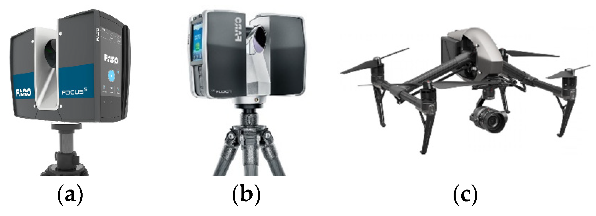
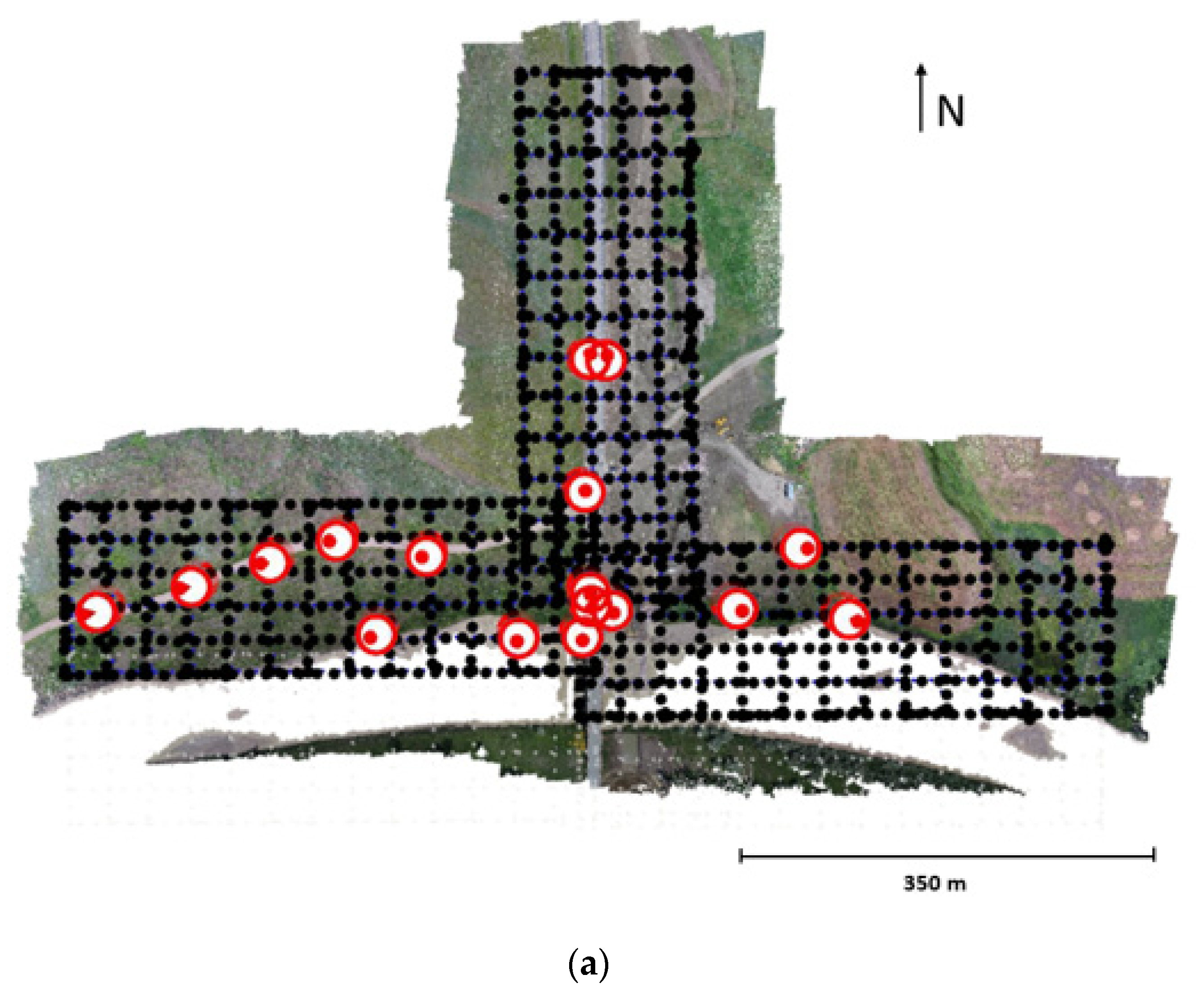
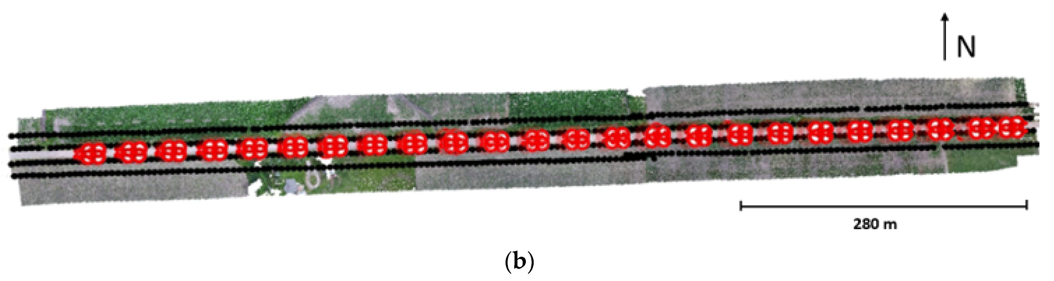
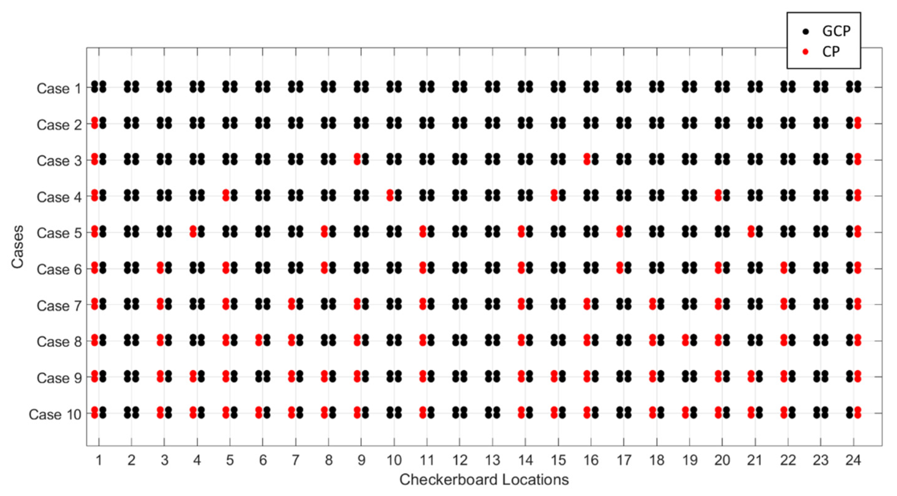
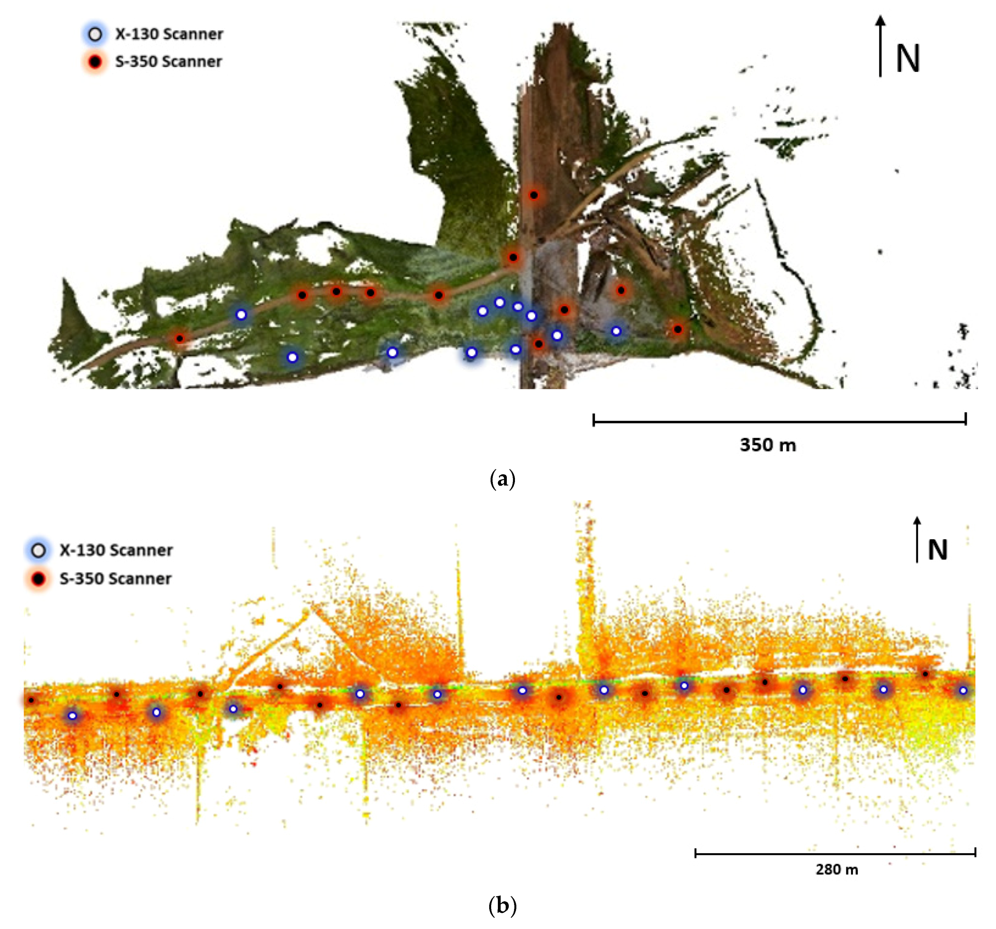
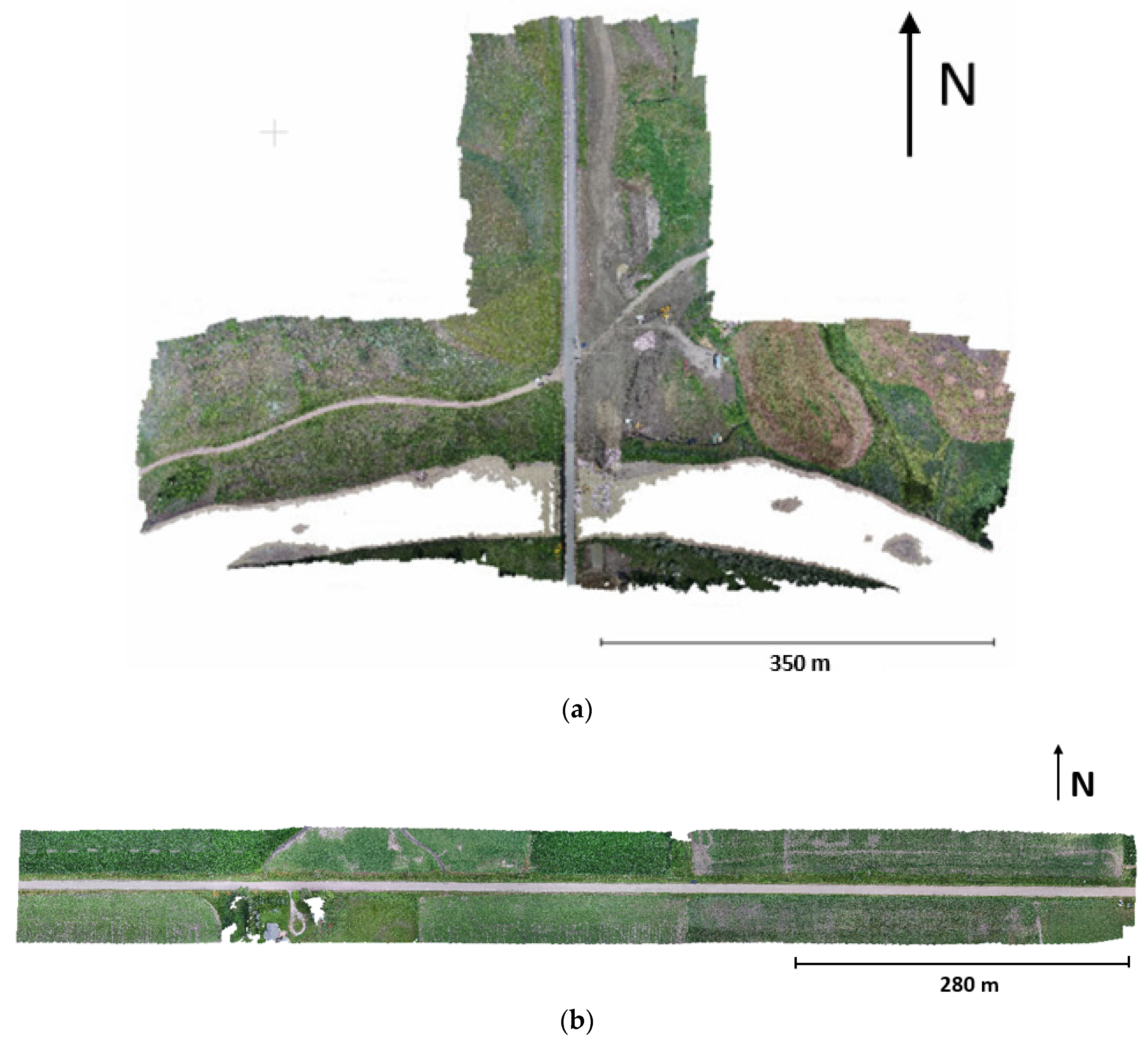
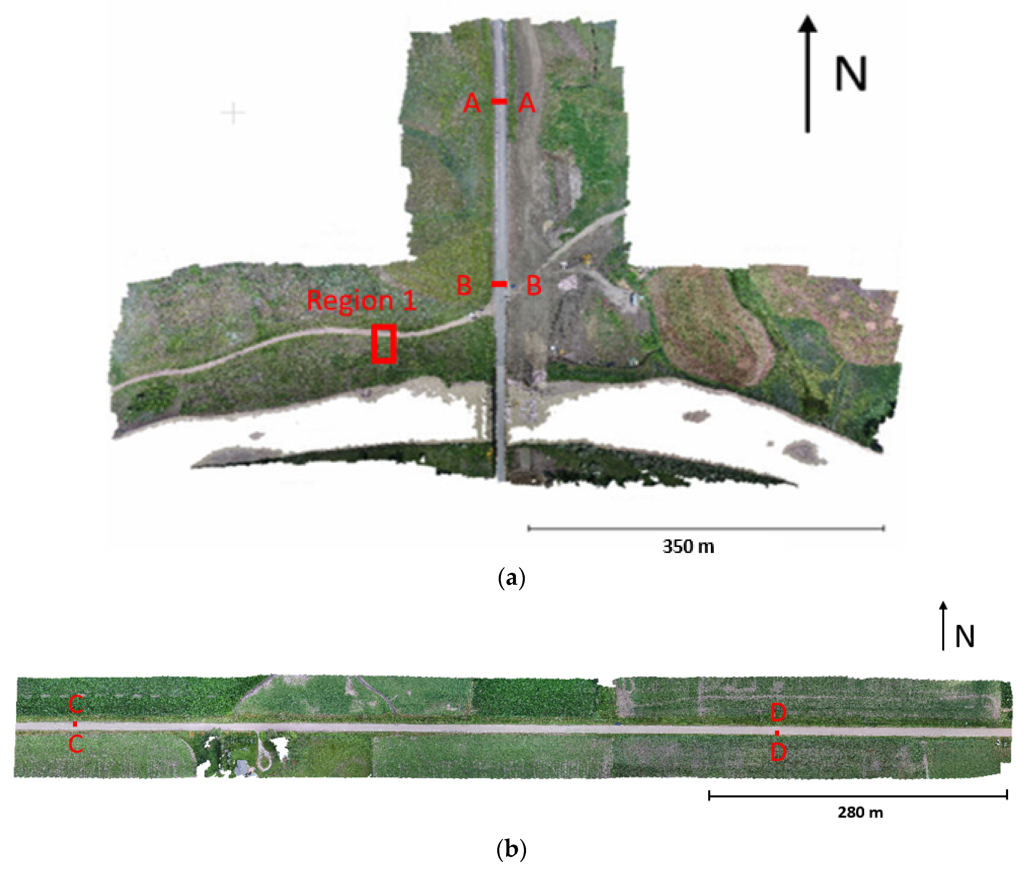
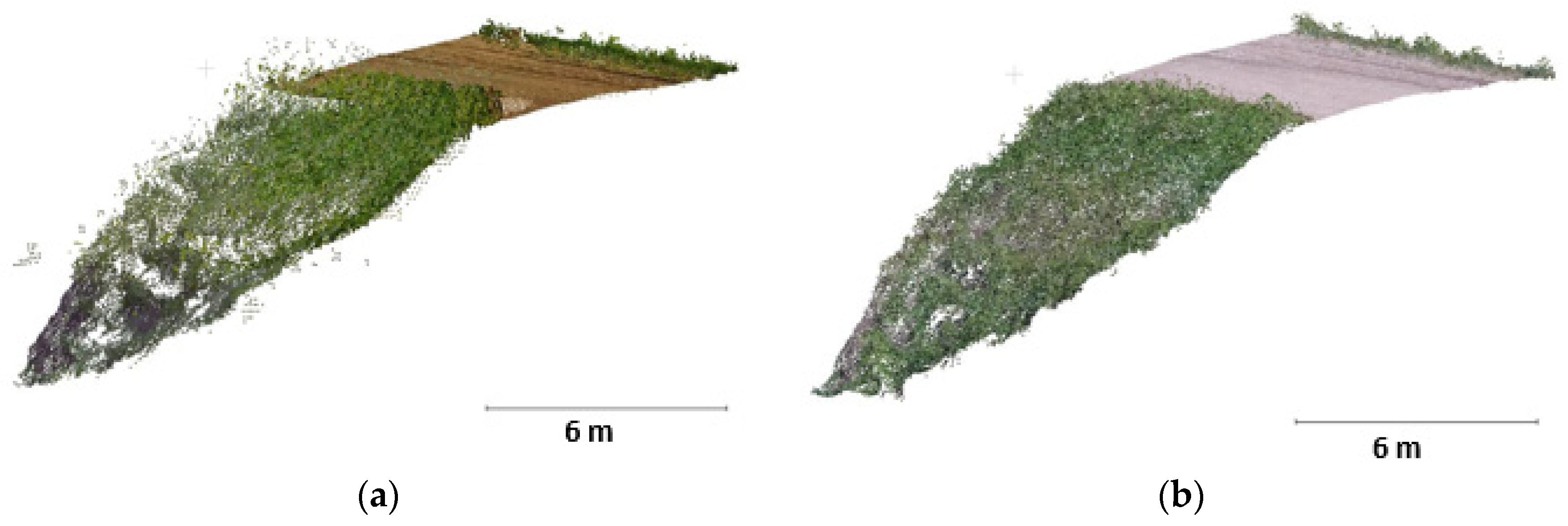
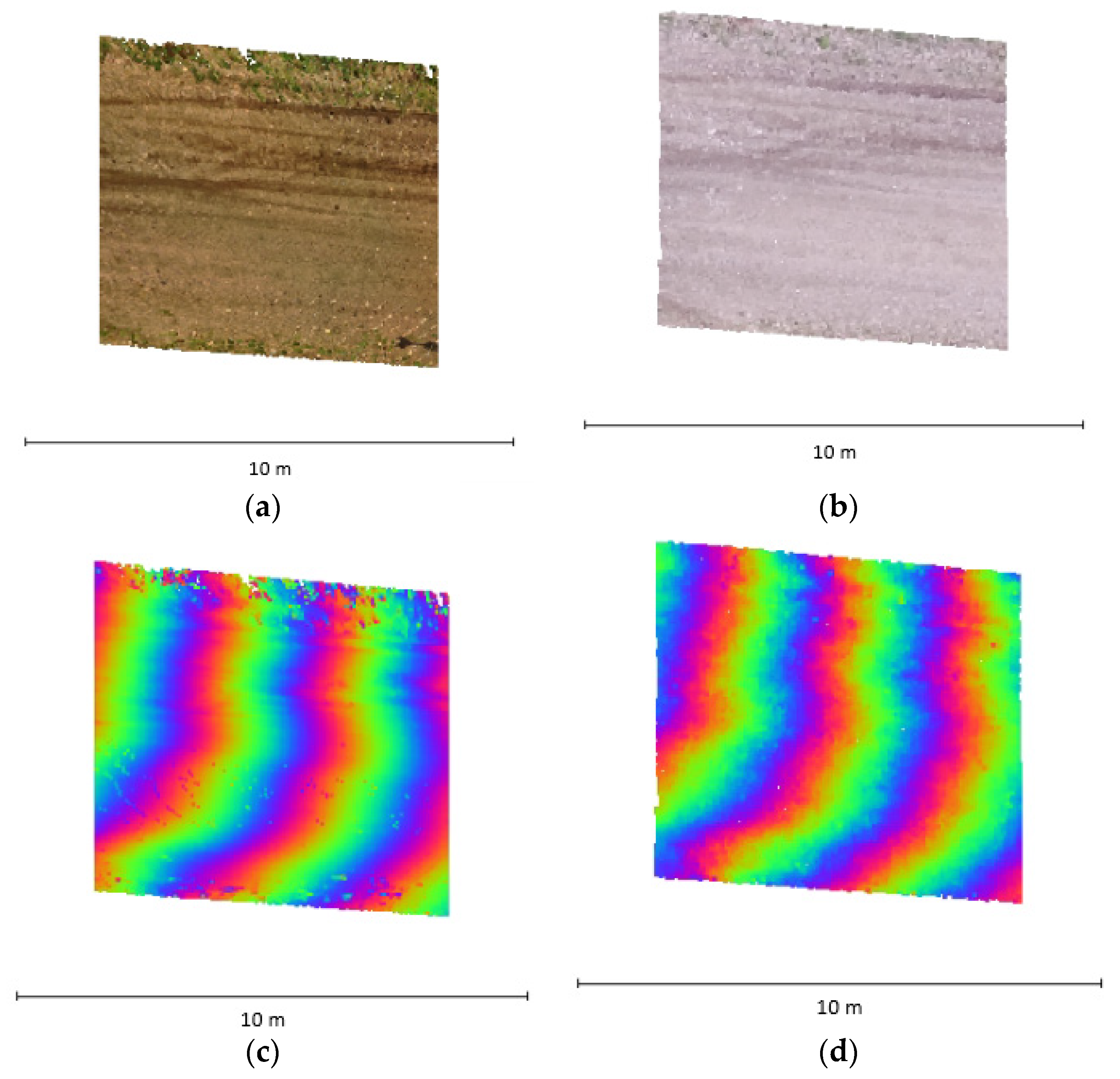
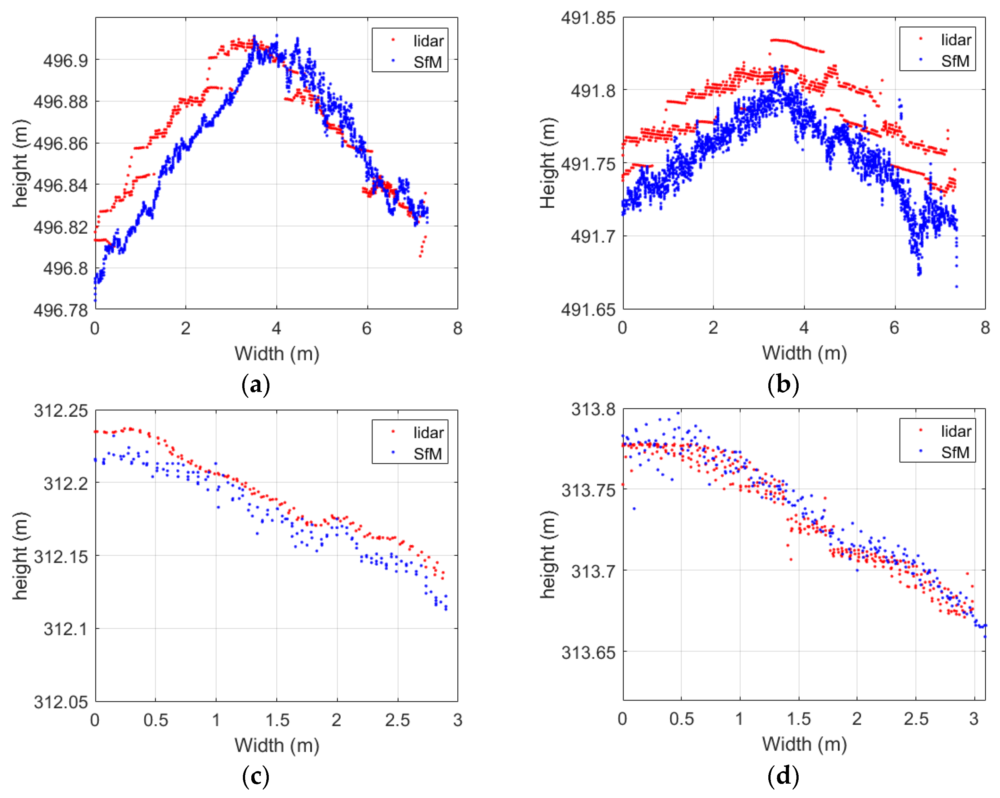
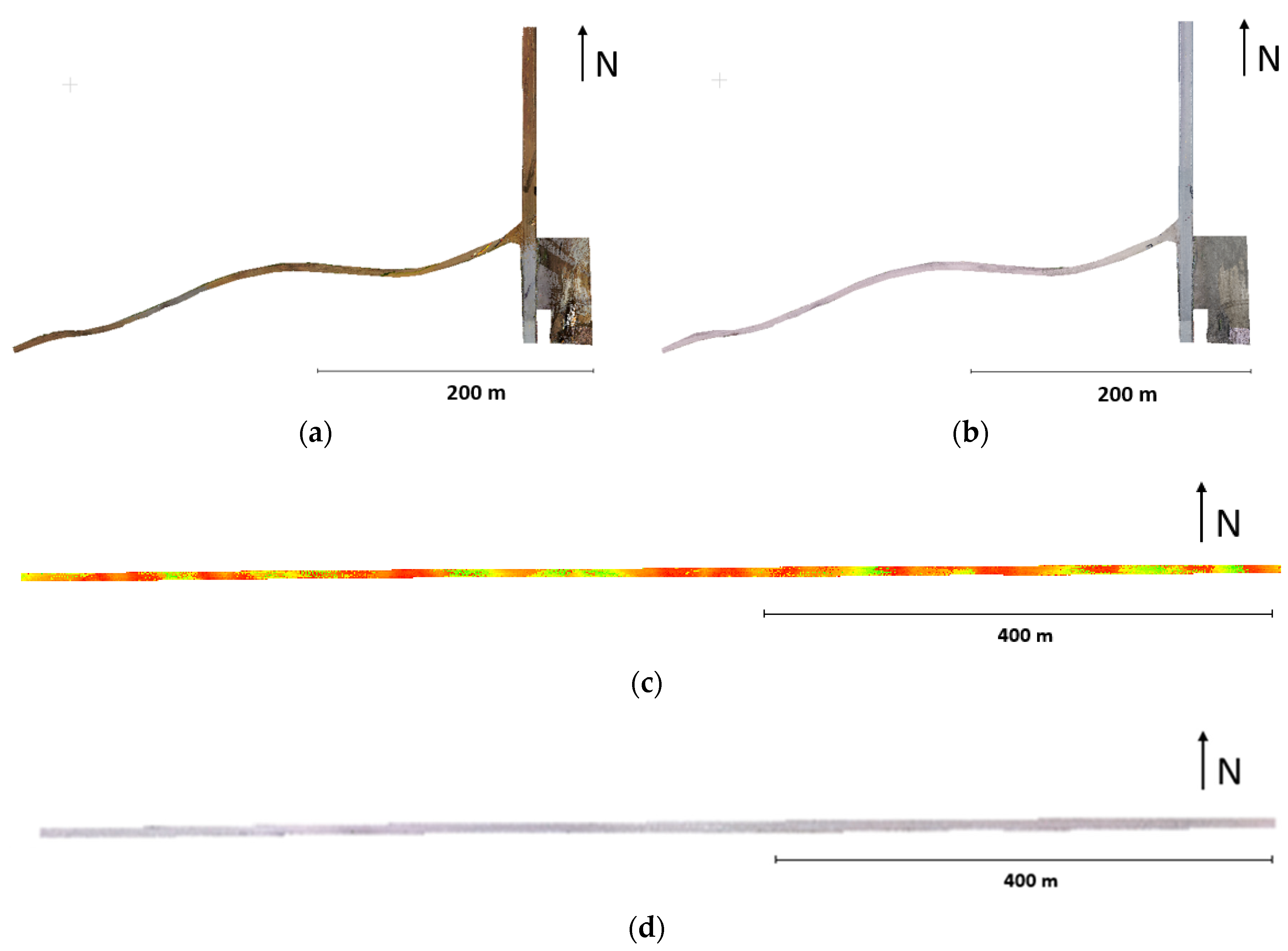
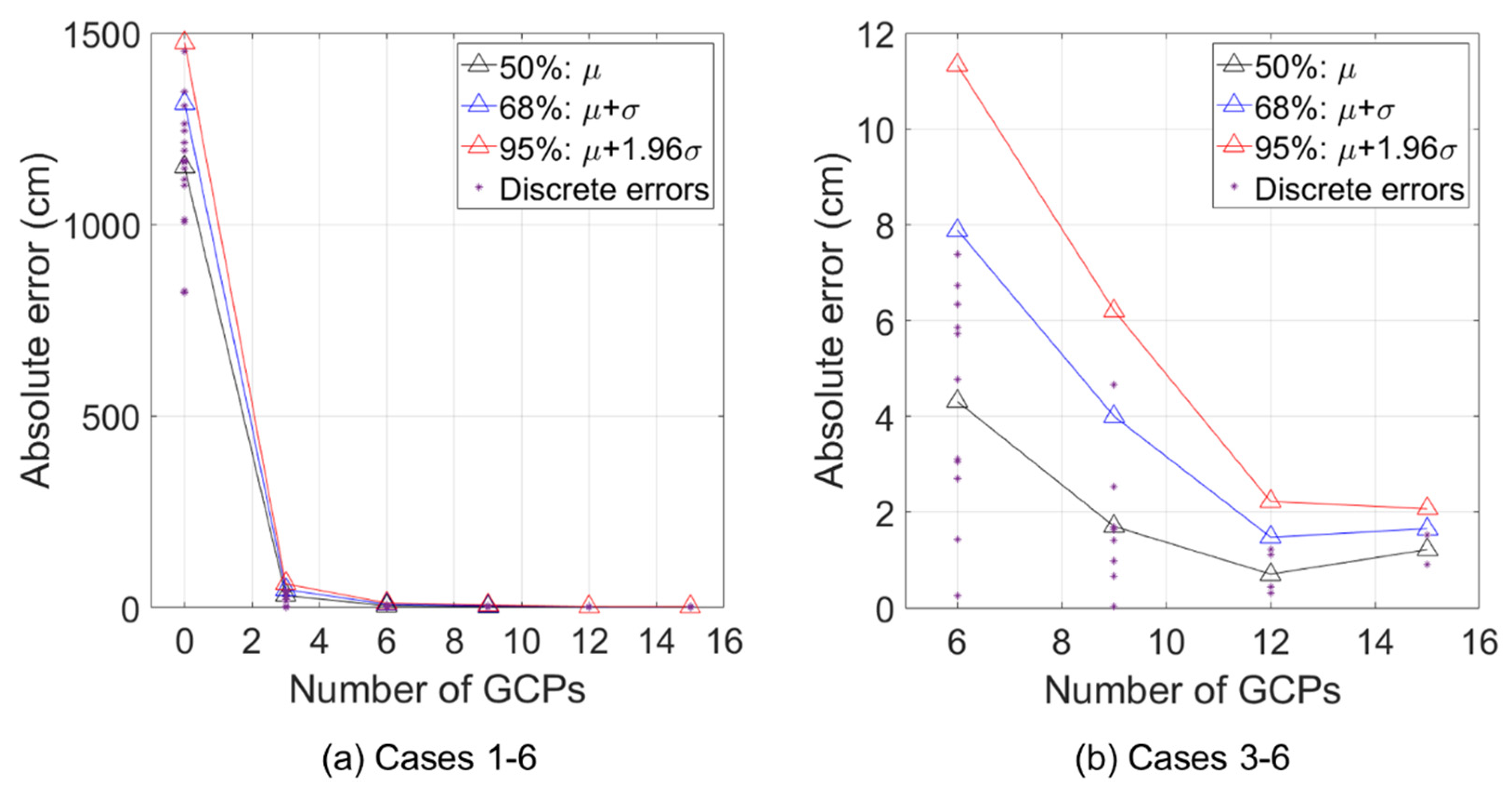
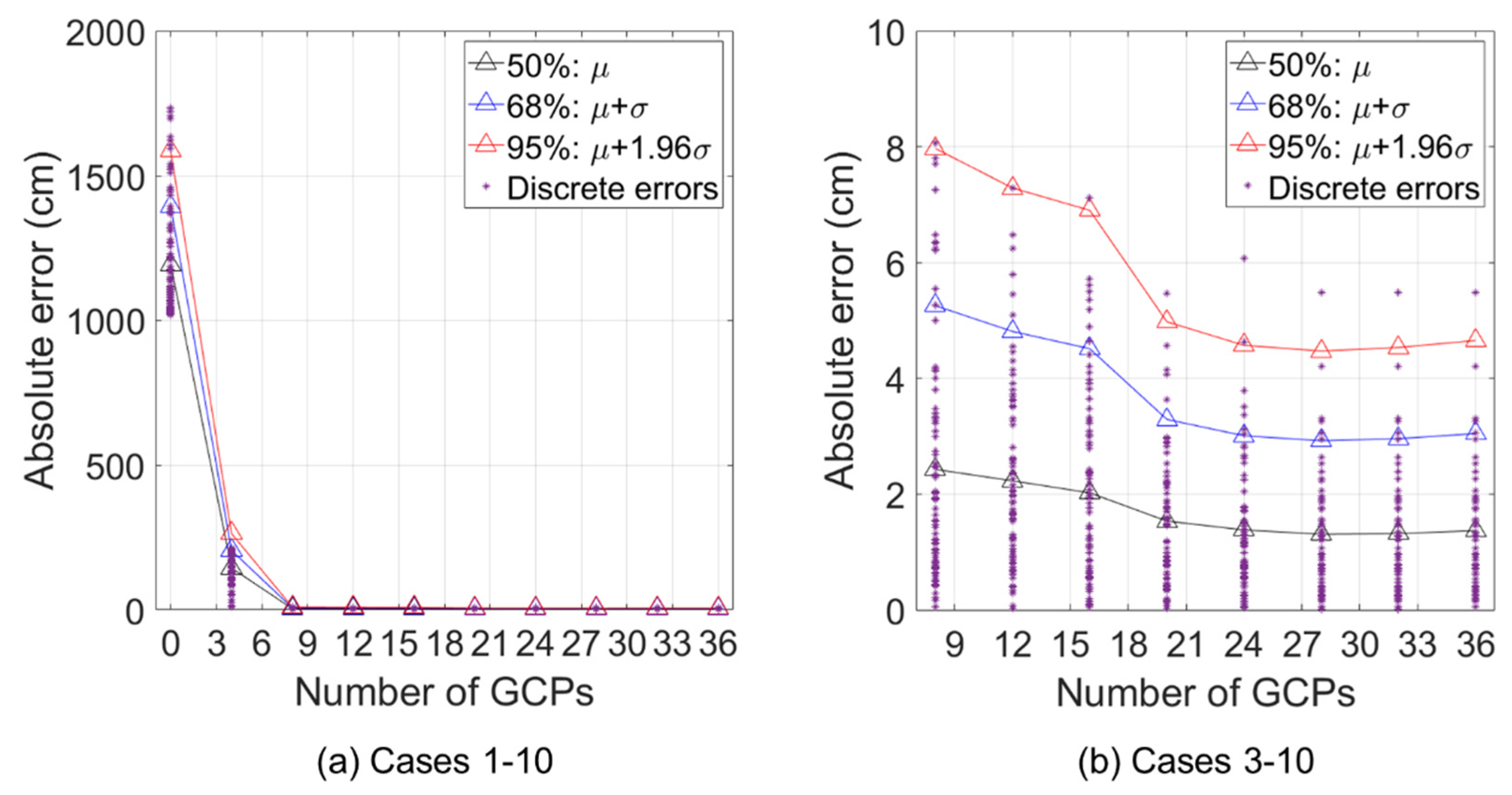
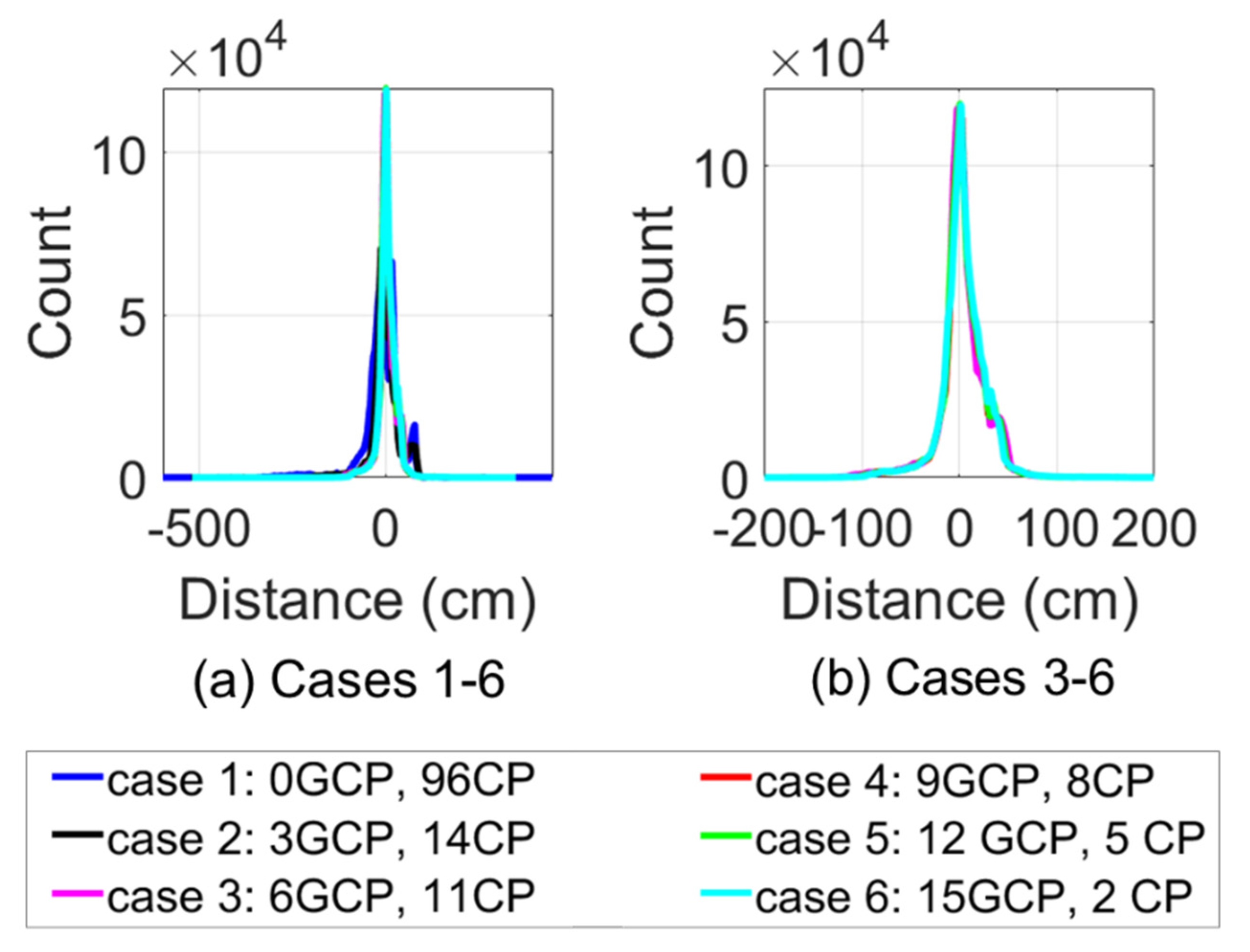
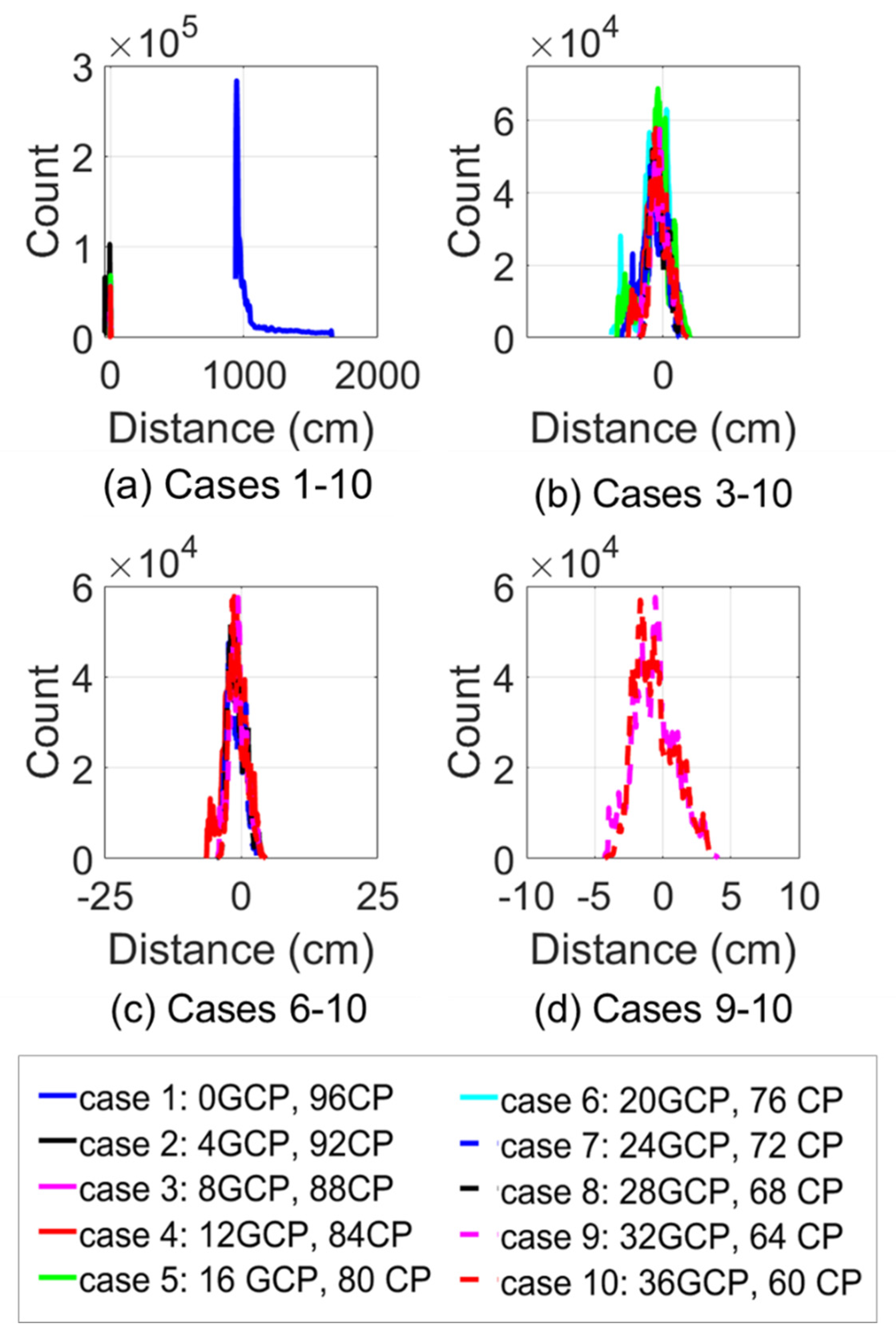
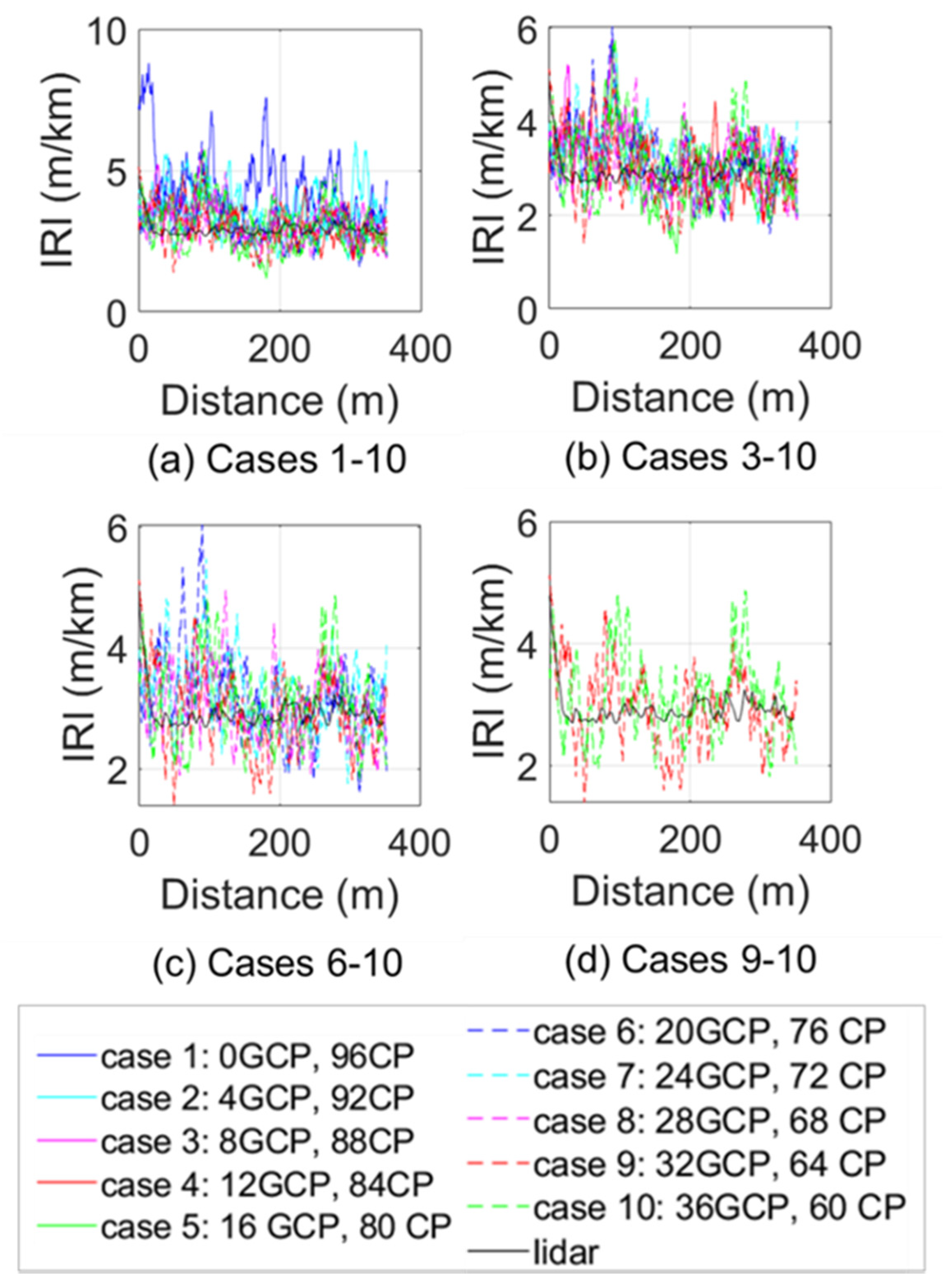
Table 1.
Ground control point (GCP) and checkpoint (CP) layout for the two sites.
| Site | Case | Target Count | GCP Count | CP Count | GCP Count to Target Count (%) |
|---|---|---|---|---|---|
| 1 | 1 | 17 | 0 | 17 | 0.0 |
| 1 | 2 | 17 | 3 | 14 | 17.6 |
| 1 | 3 | 17 | 6 | 11 | 35.3 |
| 1 | 4 | 17 | 9 | 8 | 52.9 |
| 1 | 5 | 17 | 12 | 5 | 70.6 |
| 1 | 6 | 17 | 15 | 2 | 88.2 |
| 2 | 1 | 96 | 0 | 96 | 0.0 |
| 2 | 2 | 96 | 4 | 92 | 4.2 |
| 2 | 3 | 96 | 8 | 88 | 8.3 |
| 2 | 4 | 96 | 12 | 84 | 12.5 |
| 2 | 5 | 96 | 16 | 80 | 16.7 |
| 2 | 6 | 96 | 20 | 76 | 20.8 |
| 2 | 7 | 96 | 24 | 72 | 25.0 |
| 2 | 8 | 96 | 28 | 68 | 29.2 |
| 2 | 9 | 96 | 32 | 64 | 33.3 |
| 2 | 10 | 96 | 36 | 60 | 37.5 |
Table 2.
Width and slope comparisons at extracted sections for site 1.
| Section | Average Width (m) | Average Slope (%) | ||
|---|---|---|---|---|
| Lidar | SfM | Lidar | SfM | |
| A-A | 3.65 | 3.67 | 2.4 | 2.7 |
| B-B | 3.66 | 3.67 | 2.2 | 2.4 |
Table 3.
Width and slope comparisons at extracted sections for site 2.
| Section | Calculated Slope (%) | Digital Level Measurement (%) | |
|---|---|---|---|
| Lidar | SfM | ||
| C-C | 4.08 | 4.12 | 4.0 |
| D-D | 3.36 | 3.58 | 3.3 |
Table 4.
The area under the curve and other metrics for site 1 1.
| Quantity | Case 1 | Case 2 | Case 3 | Case 4 | Case 5 | Case 6 |
|---|---|---|---|---|---|---|
| Second moment of area (1 × 107 cm4) | 3.59 | 2.74 | 1.84 | 1.80 | 1.79 | 1.82 |
| Mean (cm) | 9.17 | 0.04 | 3.49 | 4.29 | 4.16 | 4.56 |
| Mode (cm) | 11.91 | 11.77 | 1.89 | 2.95 | 1.03 | 1.97 |
| Standard deviation (cm) | 51.27 | 38.50 | 26.60 | 25.68 | 25.42 | 25.45 |
| Error at 95% CI (cm) | 12.56 | 9.43 | 6.52 | 6.29 | 6.23 | 6.23 |
1 The lowest error values are bold and underlined.
Table 5.
The area under the curve and other metrics for site 2 1.
| Quantity | Case 1 | Case 2 | Case 3 | Case 4 | Case 5 | Case 6 | Case 7 | Case 8 | Case 9 | Case 10 |
|---|---|---|---|---|---|---|---|---|---|---|
| Second moment of area (1 × 106 cm4) | 5542.41 | 113.35 | 12.14 | 10.43 | 10.82 | 9.36 | 7.66 | 7.24 | 6.98 | 6.99 |
| Mean (cm) | 1081.14 | 23.03 | 1.49 | 1.10 | 1.18 | 1.103 | 1.01 | 0.77 | 0.60 | 0.58 |
| Mode (cm) | 945.03 | 6.64 | 0.67 | 0.57 | 0.88 | 1.27 | 1.87 | 1.93 | 0.55 | 1.65 |
| Standard deviation (cm) | 188.5 | 13.11 | 2.78 | 2.38 | 2.62 | 1.99 | 1.45 | 1.45 | 1.55 | 1.49 |
| Error at 95% CI (cm) | 46.19 | 3.21 | 0.68 | 0.58 | 0.64 | 0.49 | 0.36 | 0.36 | 0.38 | 0.37 |
1 The lowest error values are bold and underlined.
Table 6.
IRI metrics for site 2 1.
| Quantity | Lidar | Case 1 | Case 2 | Case 3 | Case 4 | Case 5 | Case 6 | Case 7 | Case 8 | Case 9 | Case 10 |
|---|---|---|---|---|---|---|---|---|---|---|---|
| Mean (m/km) | 2.94 | 4.41 | 3.72 | 3.20 | 3.16 | 2.96 | 3.21 | 3.24 | 3.02 | 2.94 | 3.10 |
| Median (m/km) | 2.87 | 4.24 | 3.55 | 3.07 | 3.04 | 2.81 | 3.12 | 3.18 | 2.94 | 2.87 | 3.04 |
| Mode (m/km) | 2.56 | 3.72 | 2.45 | 2.54 | 2.51 | 2.16 | 2.57 | 2.65 | 2.05 | 2.20 | 2.31 |
| Standard deviation (m/km) | 0.33 | 1.67 | 1.13 | 1.00 | 0.77 | 1.00 | 0.94 | 0.94 | 0.83 | 0.88 | 0.93 |
1 Closest values to lidar baseline are bold and underlined.
Publisher’s Note: MDPI stays neutral with regard to jurisdictional claims in published maps and institutional affiliations. |
© 2020 by the authors. Licensee MDPI, Basel, Switzerland. This article is an open access article distributed under the terms and conditions of the Creative Commons Attribution (CC BY) license (http://creativecommons.org/licenses/by/4.0/).
Share and Cite
MDPI and ACS Style
Liao, Y.; Wood, R.L. Discrete and Distributed Error Assessment of UAS-SfM Point Clouds of Roadways. Infrastructures 2020, 5, 87. https://0-doi-org.brum.beds.ac.uk/10.3390/infrastructures5100087
AMA Style
Liao Y, Wood RL. Discrete and Distributed Error Assessment of UAS-SfM Point Clouds of Roadways. Infrastructures. 2020; 5(10):87. https://0-doi-org.brum.beds.ac.uk/10.3390/infrastructures5100087
Chicago/Turabian StyleLiao, Yijun, and Richard L. Wood. 2020. "Discrete and Distributed Error Assessment of UAS-SfM Point Clouds of Roadways" Infrastructures 5, no. 10: 87. https://0-doi-org.brum.beds.ac.uk/10.3390/infrastructures5100087