Use of Deep Learning to Study Modeling Deterioration of Pavements a Case Study in Iowa


1
Institute for Transportation, Iowa State University, Town Engineering Building, 394 Town Engineering, Ames, IA 50011, USA
2
Applied Research Associates (ARA), Transportation Infrastructure Division (Champaign Office) 100 Trade Centre Drive Suite 200, Champaign, IL 61820-7233, USA
*
Author to whom correspondence should be addressed.
Infrastructures 2020, 5(11), 95; https://0-doi-org.brum.beds.ac.uk/10.3390/infrastructures5110095
Submission received: 27 September 2020
/
Revised: 29 October 2020
/
Accepted: 30 October 2020
/
Published: 5 November 2020
(This article belongs to the Special Issue Pavement Management: Inspection and Life-Cycle Assessment)
Abstract
:This paper describes the process and outcome of deterioration modeling for three different pavement types (asphalt, concrete, and composite) in the state of Iowa. Pavement condition data is collected by the Iowa Department of Transportation (DOT) and stored in a Pavement-Management Information System (PMIS). In the state of Iowa, the overall pavement condition is quantified using the Pavement Condition Index (PCI), which is a weighted average of indices representing different types of distress, roughness, and deflection. Deterioration models of PCI as a function of time were developed for the different pavement types using two modeling approaches. The first approach is the long/short-term memory (LSTM), a subset of a recurrent neural network. The second approach, used by the Iowa DOT, is developing individual regression models for each section of the different pavement types. A comparison is made between the two approaches to assess the accuracy of each model. The results show that the LSTM model achieved a higher prediction accuracy over time for all different pavement types.
1. Introduction
Public agencies use pavement management systems (PMSs) to make objective decisions and conduct activities for maintaining pavements in acceptable conditions at minimal cost [1]. Since the early 1970s, departments of transportation (DOTs) and other transportation agencies have been implementing and establishing PMSs to match their needs, achieving significant savings and improvement in network conditions [2]. The Arizona DOT, for example, saved $14 million and $101 million during the first year and the first four years of PMS implementation, respectively [3]. The Colorado Department of Transportation (CDOT) uses PMS to efficiently spend its $740 million annual budget for maintaining and preserving more than 9100 center-line miles (about 23,000 total lane miles) [4]. It appears that there is potential for all such expenses to be more effective if PMS improvements can be developed and implemented.
A major component of any PMS is evaluation and modeling of pavement conditions at the network level. Recently, most states have begun to use automated pavement-condition surveying tools that generate images from remote sensors to collect distress information and report individual distresses through an overall condition index [5]. The concept of Pavement Condition Index (PCI), was developed by the U.S. Army Corps of Engineers in 1970 based on different types of distresses and severity levels [6]. Since then, most DOTs and related agencies have been using the PCI to evaluate pavement conditions. The PCI provides important information to pavement engineers by describing overall pavement condition based on different types of distress, roughness, and deflection [7]. The PCI is defined as a numerical rating between 0 and 100, with 0 being the worst condition and 100 the best condition for pavement segments. Based on monitored and modelled PCI values and other important condition indices, decision-makers can evaluate the functionality of pavement networks, predict the best time for maintenance and rehabilitation activities, and estimate future funding needs [8].
Long and short-term planning of maintenance and rehabilitation activities is the major tool for maximizing proper network conditions at the lowest possible cost and requires accurate and robust deterioration models for pavement networks. A deterioration model (DM) predicts future pavement conditions and helps agencies identify the most effective maintenance and rehabilitation activities [9,10], and such planning and optimization become more critical when agencies face budget reduction or are otherwise budget constrained [3].
Deterministic, probabilistic, neural network-based, and knowledge-based performance models have been used in pavement management to predict future conditions of pavement sections [11]. Currently, the Iowa Department of Transportation (Iowa DOT) forecasts the future conditions of pavement sections based on individual deterministic regression models for each pavement section. Deterministic models assume that the described process is nonrandom and that observed differences between predicted and measured values are due to random noise in the observation process.
A deterministic model will thus always produce the same output from a given starting condition or initial state. Most deterministic models are based on explicit regression expressions and are categorized into the empirical models, mechanistic models, and mechanistic-empirical models [12,13,14,15].
Probabilistic models are another group of pavement performance models, an alternative to deterministic models that do not provide probabilistic distribution of existing values. Markov probabilistic modeling uses samples of probabilistic models, with the transition process represented by a pavement–performance curve [12]. Using information from the pavement’s “before” state, the Markov process predicts the “after” state [9]. The Markov transition method is useful in network-level applications where neither historical data nor good regression equations are available [16].
In addition to Markov models, there are other types of probabilistic models like Bayesian decision models, Bayesian regression models, and semi-Markov models, which generate survivor curves [17]. The greatest advantages of probabilistic models are their capability for capturing uncertainty in the pavement prediction model, and for producing more realistic results than deterministic models.
Over the past few years, neural network (NN) applications have received greater attention, and many research studies on the application of NNs in transportation and civil engineering have been published [18,19,20,21]. Because of their capability for interconnecting neurons between layers, NN applications can often solve complex problems more efficiently than traditional methods [22]. The capabilities of neural network models for solving problems from several pavement-engineering categories are as follows [7]:
- Classification: Supervised learning in neural networks can be used to deal with unknown inputs. Neural network models have been used to investigate the classification of pavement distresses from digital images [23]. Another research study by [24] reported using a neural network to detect pavement cracks.
- Performance Prediction: Neural networks have been used in various studies as powerful and versatile computational tools for both determining the performance of existing pavement systems and predicting future conditions. The Pavement Distress Index (PDI), based on surface thickness, pavement age, and traffic level, was predicted using an NN model that outperformed other multiple-linear regressions [25]. A back-propagation neural network model was developed by [26] for predicting IRI based on pavement distress.
- Optimization and maintenance strategies: Neural networks have been used as computational tools to determine which maintenance and rehabilitation actions should be performed on deteriorated pavement sections, using a hybrid NN and genetic algorithm method developed for optimizing the maintenance strategy of flexible pavements [27].
- Distress Prediction: Neural networks can help pavement engineers predict future distresses, and a multi-layer perceptron back-propagation NN with one hidden layer has been used to predict future roughness distress in flexible pavements [28]. NNs could be a powerful alternative to traditional techniques that are always limited by normality, linearity, and collinearity assumptions. Two major advantages of using NNs are their ability to model complex and nonlinear large amounts of data and detect all possible interactions between predictor variables.
It should be mentioned that, because pavement deterioration happens over time, it is important to include the dependency of performance measures on historical data (time) in a prediction model. Accurate time-series prediction is also critical for abnormality detection, resource allocation, and financial planning [29]. Predicting data time-dependency is challenging because such prediction depends on external factors like weather and traffic load [30]. Time-series analysis works better with highly correlated measurements over time, because explanatory variables may fail to explain the correlation mechanisms. On the other hand, in regression analysis, the explanatory variables should sufficiently explain the trend, resulting in independent fitting residuals.
A deep-learning method designed for sequential data is the recurrent neural network (RNN) that has recently received additional attention from researchers primarily because of its capability in learning sequences [31,32,33]. RNNs have been widely applied to many time-dependent datasets for use in prediction problems like speech prediction, pattern prediction, economic prediction, and traffic prediction [34,35,36]. Since RNNs are developed to utilize historical data in time-series analysis, inclusion of a regression model that relies on explanatory variables and historical data of the response variable improved the model accuracy. These networks are designated as recurrent because future forecasting depends on both current and previous stages. Several RNN algorithms, such as the long short-term memory (LSTM) network, have been developed over the past two decades. LSTM was introduced to support modeling and forecasting of long-term data series. The network was developed to overcome the vanishing gradient problem in which algorithms tend to accumulate errors when a long string of observations are added as predictor variables, increasing prediction variability and associated total error. Based on the literature, another RNN network called the gated recurrent unit (GRU) also solved the vanishing gradient problem, but the LSTM outperformed the GRU in many details [37].
In this research, the LSTM method was used for time-dependent prediction of the pavement condition index. This network is suitable for pavement applications because the data is presented in time series with both low observation frequency and high levels of variability. The goal of this study was to develop a new robust deterioration model suitable for long-term forecasting, in which the model performance can be objectively evaluated. An LSTM network will utilize historical pavement condition records of the Iowa DOT (PMIS) in the time span between 1998 and 2018. The new time series algorithm, a deep-learning approach specifically developed by LSTM networks, was used to predict future conditions of the three different pavement types in the state of Iowa. The Keras software package, a high-level neural network API written in Python, was used for generating the LSTM model, with a focus on enabling fast experimentation. This package uses a deep-learning open-source library based on the TensorFlow software library. The performance and results of the new algorithm are compared to the current method used by Iowa DOT for deterioration modeling.
2. Methods
Figure 1 shows the steps required to be completed in the proposed method, with the individual steps described in detail in the following subsections.
2.1. Data Collection
To develop and implement the new framework, historical records of pavement condition data were acquired from the Iowa DOT (PMIS). These data were collected for Iowa’s interstate and primary network since 1997, the year in which the Iowa DOT began collecting automated pavement distress data [38]. The data used in this study were acquired between 1998 and 2018, and include information regarding highway system classification, construction and reconstruction dates, unique section identifiers, traffic levels, automated pavement distress data, and pavement ride quality. The pavement types included in the study were asphalt concrete (AC), Portland cement concrete (PCC), and composite (COM) pavements.
The pavement distress information collected includes rutting and cracking, data such as transverse cracking, longitudinal cracking, alligator cracking, wheel-path cracking, and patching, with low-, medium-, and high-severity levels assigned to cracking data for all pavement types. For AC and COM pavements, rutting was reported as the average rut depth in both wheel paths, and for PCC pavements, faulting was estimated using the acquired longitudinal profile. The international roughness index (IRI) was also used to characterize ride quality for all pavement types. Pavement condition data is collected in two-year cycles in which half the network is surveyed every other year. The Iowa DOT spends about $1 million annually on collecting pavement condition data [8].
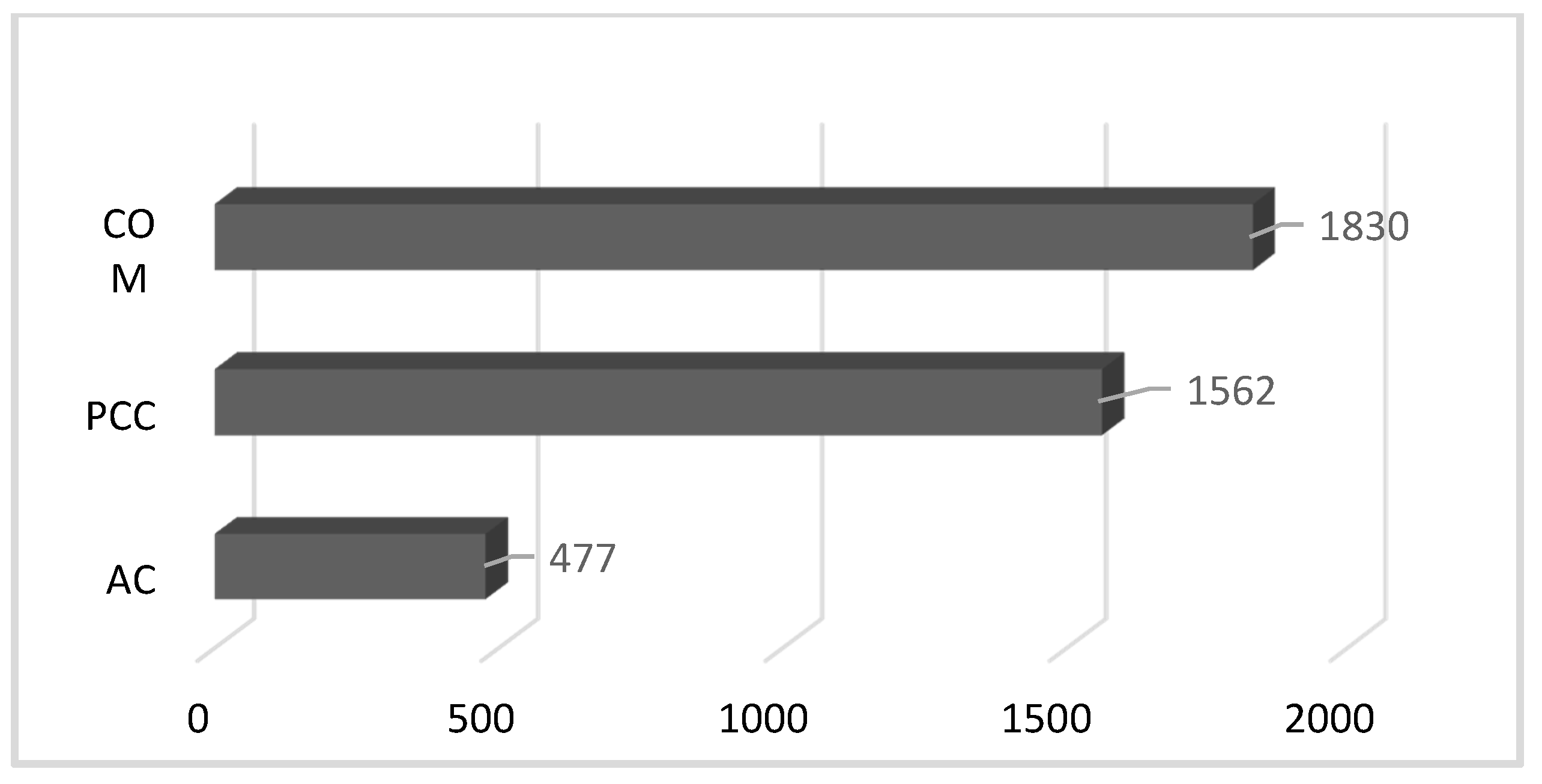
In many cases, minor maintenance and rehabilitation records were not available, so the maintenance impact on pavement condition over time was not modelled in this study. Moreover, segments with PCI values increasing over time were discarded from the analysis because they might be associated with unrecorded maintenance activities. A 10-point PCI increase was arbitrarily considered to be a normal fluctuation due to measurement errors or seasonal impacts. Figure 2 shows the number of different sections for each pavement type, with the descriptive statistics for each pavement type given in Table 1. The total number of data records for all of the 20-year time frame was comprised of 3805 AC records, 14,117 COM records, and 13,123 PCC records.
2.2. Preprocessing
After collecting and arranging the data based on pavement type, condition indices were estimated using the reported condition data. Pavement condition can be summarized using four scaled indices with values ranging from 0 to 100, with 0 corresponding to the worst condition and 100 to the best condition. These indices can then be used to calculate the overall PCI using the same scale for individual indices, resulting in the definition of a global index for comparing different pavement types. In this study, the indices were calculated based on definitions provided in a previous study for the Iowa DOT [8] and included:
- Riding index;
- Rutting index (AC and COM Only);
- Cracking index;
- Faulting index (PCC Only).
In AC and COM pavements, four different cracking sub-indices were used to calculate the cracking index; these included transverse, longitudinal, alligator, and longitudinal-wheel-path cracking. Only two sub-indices, transverse and longitudinal cracking, were used to characterize PCC pavements. Three severity levels were used by the Iowa DOT in evaluating pavement distresses, with 1, 1.5, and 2 coefficient values, used for low-, medium-, and high-aggregated severities, respectively. All severity levels were then converted into low severity. Since a maximum value (threshold) corresponds to a deduction of 100 points, a cracking sub-index of 0 was determined for each crack type within pavement type, and all threshold values were extracted from a previous Iowa DOT study [8]. Table 2 and Table 3 represent threshold values for the cracking sub-indices and weights for calculating the cracking index by pavement types, based on the coefficient values provided by Iowa DOT experts.
The cracking index values for all three pavement types, based on the coefficient values provided by Iowa DOT experts, were as follows:
The International Roughness Index (IRI) is the most commonly used ride-quality index. The riding index used in this study was based on the IRI acquired by the Iowa DOT and expressed on a scale of 100. IRI values below 0.5 m/km were taken as a perfect 100, while values above 4.0 m/km were taken as 0 on the index scale. Other values between 0.5 and 4 m/km were calculated using linear interpolation [8]. Rutting is defined as the permanent total deformation or consolidation accumulated in an asphalt pavement surface wheel path. The rutting index from this study used rut depths available in the PMIS database, and, based on previous research, a threshold value of 12 mm corresponded to 0 on the rutting index scale of 100, and values below 12 mm were applied as corresponding deductions [8]. Faulting is defined as the difference in slab elevation across a joint or crack occurring due to differential vertical displacement between two sides. Similar to the rutting index for AC pavements, the faulting index is expressed on a scale of 100, with the faulting value equal to or greater than 12 mm set to 0 and the faulting value equal to zero set to 100 on the index scale [8].
After calculating all cracking, riding, rutting, and faulting indices for AC, COM, and PCC pavements, a weighted average formula was used to calculate the PCI values. The current formulae for calculating the PCI for AC, COM, and PCC pavements are as follows [8]:
Based on PCI values, the Iowa DOT classifies pavement condition for the interstate highway system as good, with a PCI value between 76 and 100; fair, with a PCI value between 51 and 75; and poor, with a PCI value between 0 and 50. Based on these classifications, approximately 91% and 79% of the interstate highway system and the non-interstate highway system in the state of Iowa was categorized as good-condition pavement up to the end of 2017 [39].
2.3. Developing LSTM Model
To predict the future condition of individual pavement sections, a modified RNN algorithm called LSTM was used in this research. While in conventional feed-forward neural networks, all observations are considered independent, the models in RNN consider the effects of previous observations and therefore account for the correlation between consecutive observations. It is worth mentioning that traditional RNNs can work properly only with short-term dependencies, and for making an accurate prediction with an RNN, having information from previous stages is mandatory. In fact, an RNN fails when too many inputs from historical observations are used. Observations added as predictor variables will increase variability in the predictions and the total error, a phenomenon referred to as the vanishing gradient effect.
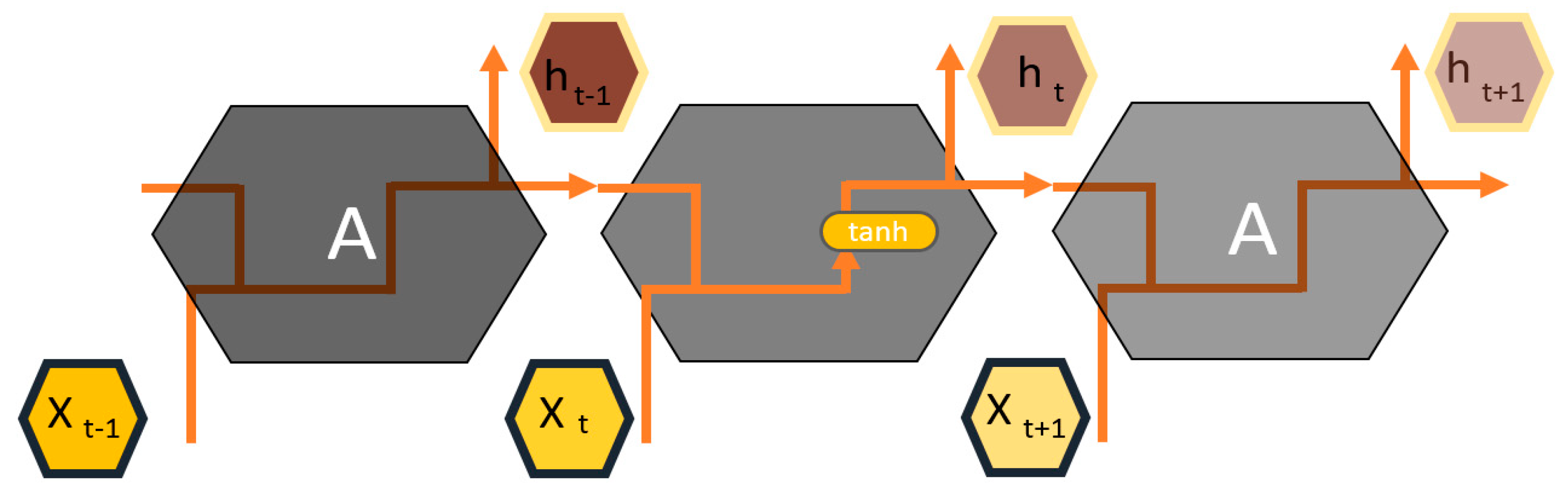
Generally, in feed-forward neural networks, the multiplication of errors from previous layers, rate of learning, and input for a layer define the updating weight for the following layer. As a result of several multiplications of the small value of activation-function derivatives (Sigmoid, Tanh, ReLU), the gradient approaches zero, increasing training complexity and causing information loss within the training layers. To overcome this limitation, LSTM was proposed as a modified version of traditional RNNs while taking advantage of the effectiveness of RNN methods. The information in LSTMs flows through a cell states mechanism in which LSTMs can selectively either forget or remember information based on its impact on model performance [40]. Figure 3 is a schematic of the repeating module in an RNN that goes through three major steps.
In the first step, the LSTM passes the output from the previous time step to the forget gate, where it is classified using the sigmoidal function shown in Equation (1) either as significant information passed to the next step in the training or insignificant information dropped from the training model [40]:
where represents the forget gate, is the Sigmoid function, represents the weight for the forget gate neurons, is the output of a previous LSTM block at time , represents the input at the current time step, and represents biases for the forget gate.
In the second step, the LSTM decides what new information should be stored in the cell state by identifying values requiring updating by the Sigmoidal function and the vector of new candidate values created by the Tanh function that could be added to the next state. These two functions are shown in Equations (2) and (3) [40]:
where represents the input gate, represents the weight for respective gate neurons, represents the input at the current time step, and represents the candidate for cell state at time step (t).
By combining information from the previous cell and the input gate from the current time step, the information for the later step will be updated. Equation (4) represents how information is filtered from the forget gate layer combined with new information from the current time step. Other Sigmoid and Tanh functions help the LSTM cell decide what information should be taken as output. Equations (5) and (6) represent the Sigmoidal and Tanh functions in the last step [40]:
where is a cell state (memory) at time step (t), represents the output gate, and represents the output of the LSTM block at time step (t).
2.4. Training
For the learning process in the LSTM algorithm, the dataset corresponding to PCC and COM pavements is divided into training (70%) and validation (30%) sets. Because the number of records in AC pavements was less than that of the two other pavement types, the database was divided into training (80%) and validation (20%) sets for AC pavements. The training dataset was used for developing the model and conducting the learning process, while the validation dataset was used for checking the accuracy of the model.
2.5. Validation
Model validation is performed to confirm that the output of the statistical model is acceptable with respect to the collected data (actual data). In order to evaluate any machine learning model, it is necessary to test the model with data not used in the training set. In this study, a Train Test split approach was used for cross-validation (CV), a validation technique that checks the effectiveness of the machine-learning model. After performing model training on 70% of the database (the training dataset), the validation dataset was used as a test sample to validate model performance.
2.6. Comparison
The LSTM model performance was compared with the sigmoidal and exponential functions used by Iowa DOT to fit deterioration models for individual sections. The accuracy of each model with respect to riding, cracking, and rutting in AC and COM pavement types, and riding, cracking, and faulting in PCC pavement types was compared for both models.
3. Results and Discussion
In the following sections, the application of each modeling approach in the databases of the three different pavement types is described and the results are presented and discussed. The overall results from both models are presented in Table 4, with the actual value of each index compared with the predicted value of the same index from the LSTM and Iowa DOT regression models.
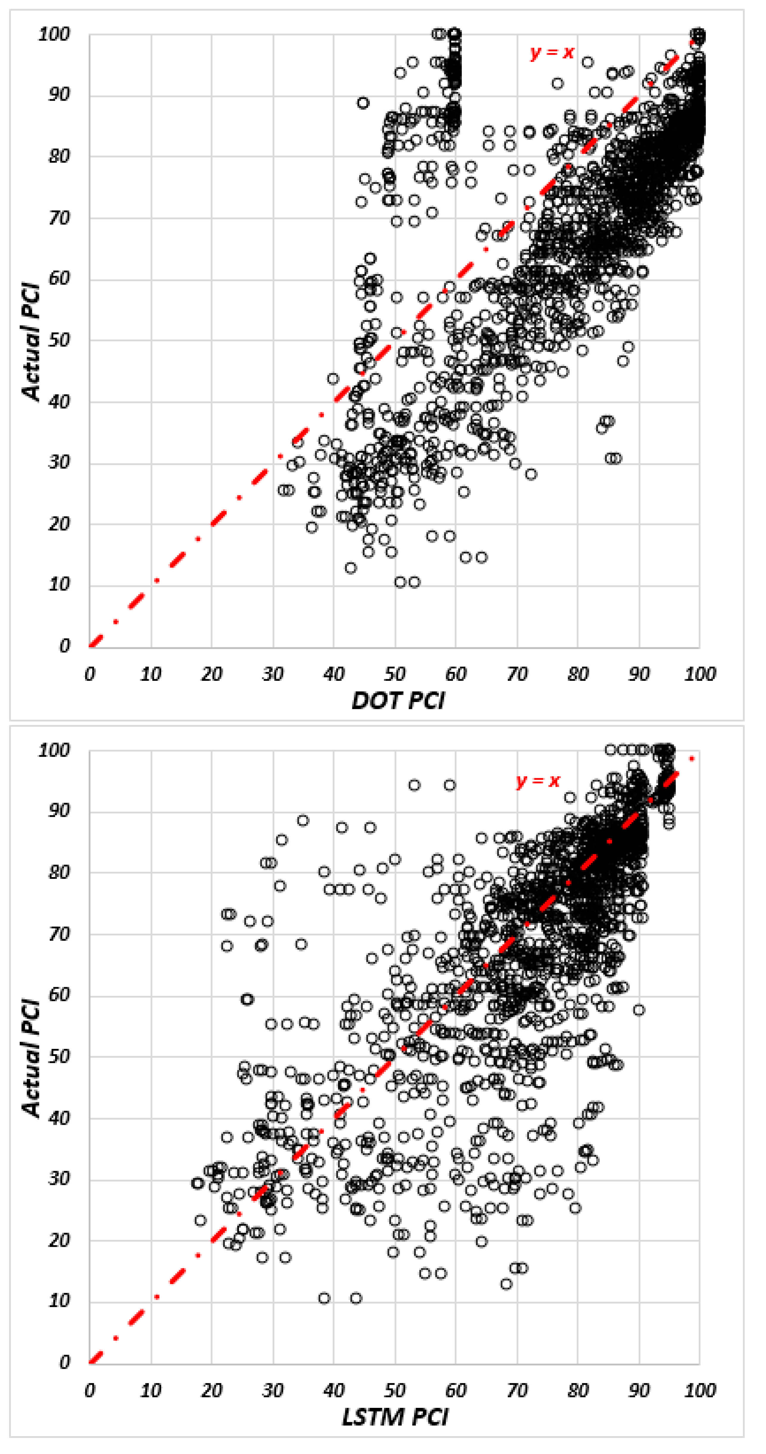
The Iowa DOT has an individual regression model for each individual section with specific factors for predicting the future condition of the pavements based on age. While the sigmoidal transformation functions were applied to cracking, rutting, and faulting indices, the exponential function was used to fit the riding index. Based on the actual and predicted values of each index, the PCI value was calculated for each pavement type. Figure 4, Figure 5 and Figure 6 present the comparisons between the actual PCI value and predicted PCI value for each pavement type in the DOT and LSTM models.
It should be noted that the evaluations of the regression models are restricted to the residuals between the fitted functions and the actual readings, although the LSTM evaluation was based on its ability to predict full performance curves not included during the training stage. For validating the prediction results of the individual regression models and comparing the results of the current Iowa DOT method with LSTM models, 50 AC, 80 PCC, and 80 COM sections were tested. The results were compared with the actual value of each index.
The comparison included models developed for AC, COM, and PCC pavements. R-square and the standard error of estimate (SEE) were considered to evaluate the accuracy of the models. The R-square and SEE functions are shown in Equations (7) and (8):
where is the actual value, is the predicted value, is the average of actual values, and N represents the number of observations.
The results for AC pavements show that the LSTM model obtained a higher prediction accuracy, compared to the individual DOT regression models. The R-square values in the LSTM models were 0.61 for the riding index, 0.19 for the rutting index, 0.35 for the cracking index, and 0.61 for the PCI while the values for the DOT models were 0.55, −5.11, 0.15, and 0.31, respectively. It is worth mentioning, that R-square is defined as the proportion of variance explained by the fit; if the fit is actually worse than just fitting a horizontal line, then R-square is negative. Additionally, the result of SEEs for both models indicates that the LSTM model obtained less standard error of estimate, compared to DOT models. The SEE values in the LSTM models were 18.66 for the riding index, 19.74 for cracking index, 13.58 for rutting index, and 12.18 for the PCI while the values for the DOT models were 20.08, 22.57, 37.40, and 16.17, respectively.
Additionally, the results for the COM pavements show that the LSTM model obtained a higher prediction accuracy. The R-square values were 0.43 for the riding index, 0.19 for the rutting index, 0.39 for the cracking index, and 0.50 for the PCI in LSTM models while the corresponding values for the DOT models were −0.02, −4.7, −0.05, and 0.11, respectively. Additionally, the SEE metrics for both models indicate that the LSTM model obtained less standard error of estimate, compared to DOT models. The SEE values in the LSTM models were 24.5 for the riding index, 15.29 for cracking index, 15.57 for rutting index, and 13.78 for the PCI while the values for the DOT models were 32.7, 19.72, 41.48, and 18.46, respectively.
Additionally, the LSTM model outperformed DOT’s regression models with respect to PCC pavements. Fluctuations in the PCC database due to maintenance activities were less than the two other pavement types. The R-square values were 0.86 for the riding index, 0.62 for the faulting index, −0.26 for the cracking index, and 0.70 for the PCI in LSTM models, and the corresponding values in the DOT models were 0.66, −3.68, 0.26, and 0.44, respectively. Additionally, the result of SEEs for both models indicates that the LSTM model obtained less standard error of estimate, compared to DOT models. The SEE values in the LSTM models were 14.71 for the riding index, 26.83 for cracking index, 12.4 for faulting index, and 12.51 for the PCI while the values for the DOT models were 22.96, 20.37, 43.35, and 17.21, respectively.
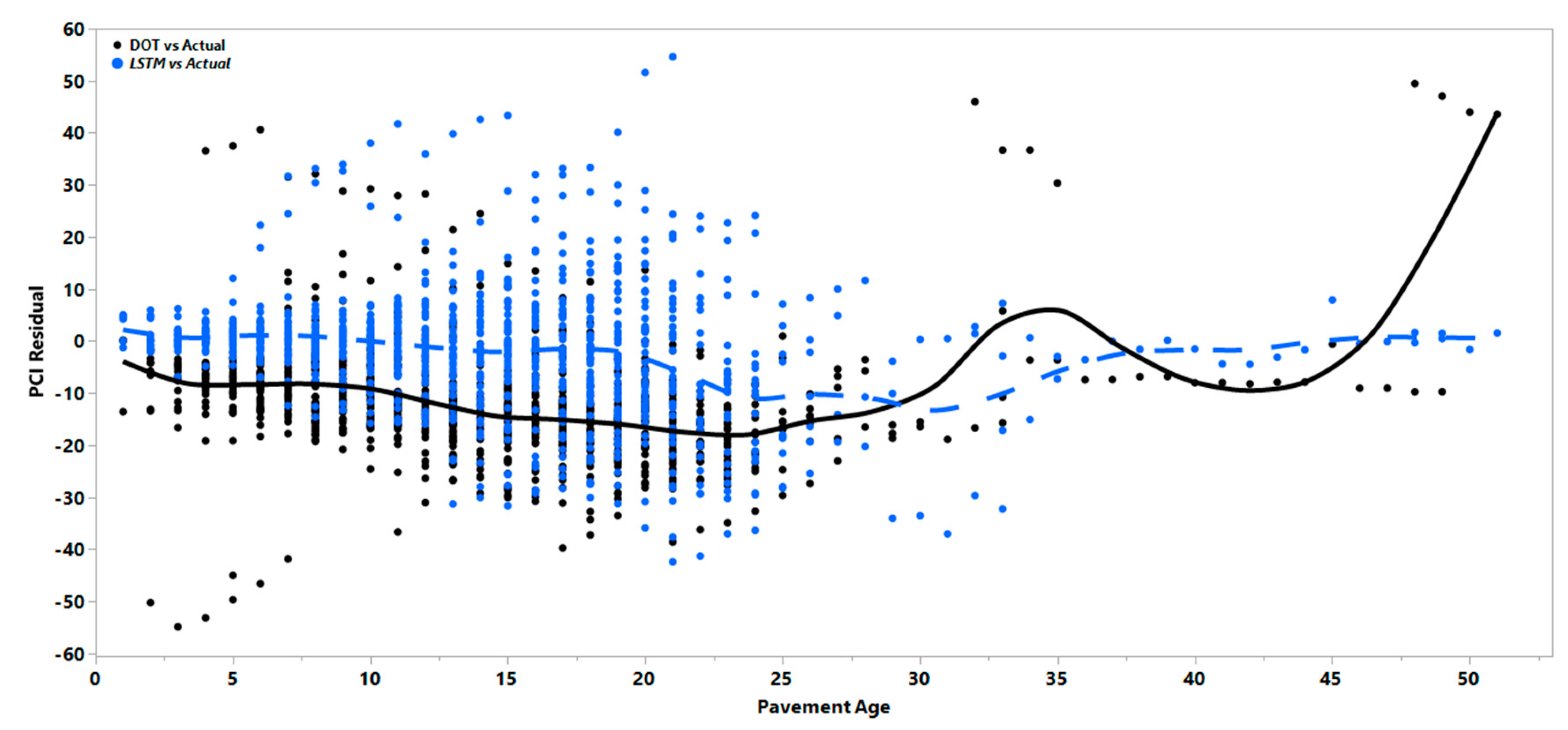
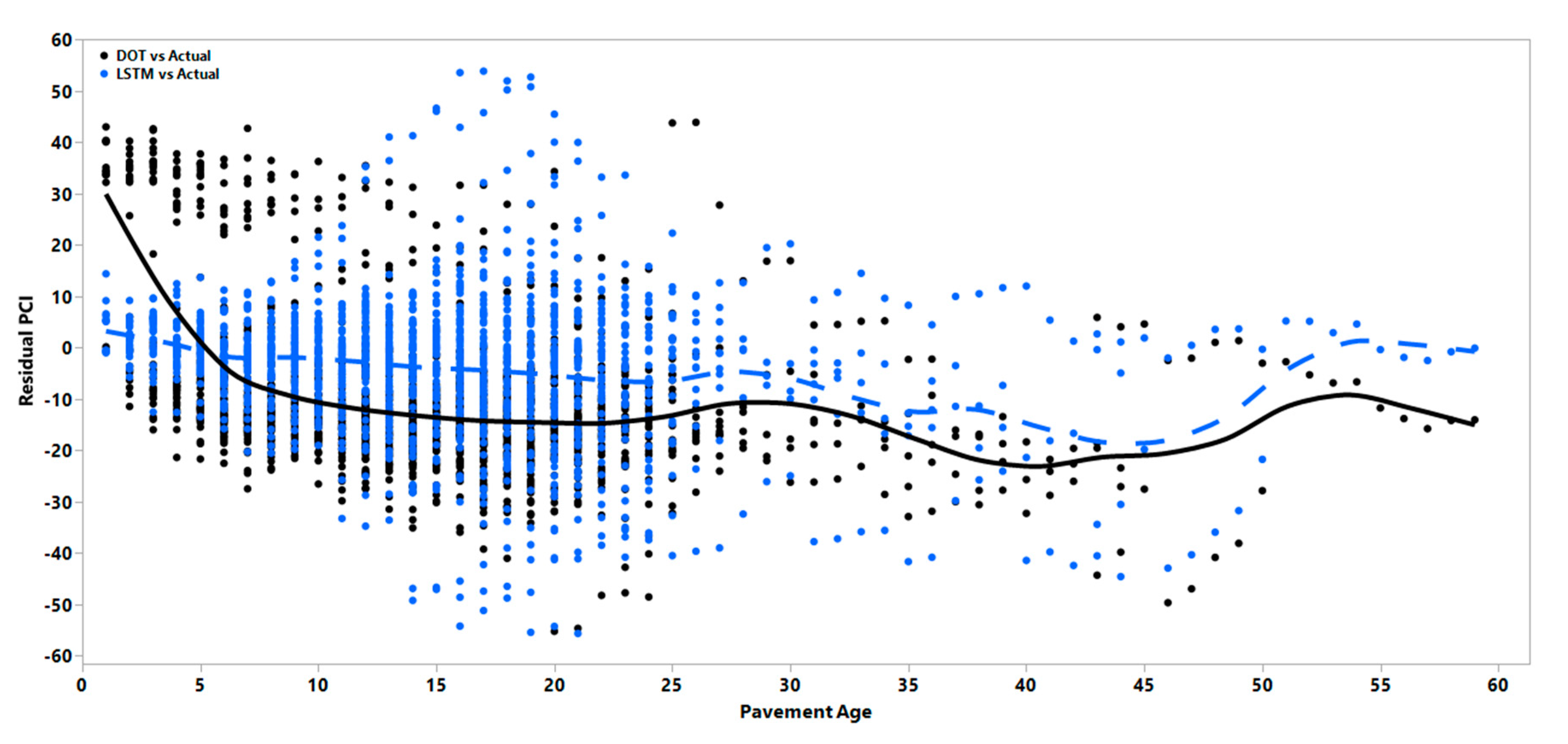
Figure 7, Figure 8 and Figure 9 also reflect the effect of age on the prediction residuals for each model in both the short- and long-term duration. These results show that the errors will more significantly widen and fluctuate after the first five years of pavement age for all three pavement types. Residuals can generally be either positive or negative; however, consistent differences between the predicted and observed values to one side of the prediction model is referred to as bias, and the variability in the mean observed value of these residuals is referred to as variance. Bias can be formally defined as the expected value of the model residuals, as shown in Equation (9):
where is the predicted value, is the observed value, and is the model residual .
As can be seen in Figure 7, Figure 8 and Figure 9, the DOT regression models show a consistently higher bias as the average line deviates from the zero value. To check whether the bias of the DOT regression model was significantly higher or lower than the LSTM model bias, a hypothesis test was performed to calculate the regression and LSTM models’ average absolute residual values. To determine the possibly unequal residual variance between the models, the Kolmogorov–Smirnov test, a non-parametric test that allows for testing with unequal variances, was performed. Results showed that the regression model had a significantly higher bias with a negative value, meaning that the regression model will consistently overestimate the index values and result in less conservative predictions. Even though the variance of the residuals increased in the LSTM over time, the mean of the residual in the LSTM model was still less than that of the regression models. The solid black line and dotted blue line in the figures show how the mean errors changed over time. Table 5 represents the mean of residuals of the PCI for the DOT and LSTM models.
4. Conclusions
The deterioration models of the historical pavement condition data for the state of Iowa were developed using an LSTM approach. The proposed model and current method in Iowa DOT were compared to investigate the model accuracy.
- The comparison between the developed model and the individual regression models used by the Iowa DOT from the three different pavement types indicates that the prediction accuracy in the LSTM model is higher than individual regression models.
- The LSTM achieved a higher PCI prediction accuracy than the individual regression models in all three pavement types.
- A hypothesis analysis of the mean was conducted for the PCI residual in both techniques and the results exhibited less LSTM bias than that of the individual regression models.
- Each of these two methods has its own advantages and disadvantages. The equation of the individual regression models requires an annual update, and each section will exhibit a new year-by-year behavior, making the prediction process more complex. The LSTM is only one more consistent model compatible for all sections using a training process. The LSTM approach was sensitive to the data fluctuation resulting from unrecorded maintenance activities.
- While the evaluation of the regression models was restricted to residuals between the fitted functions and the actual readings, the evaluation for the LSTM was based on its ability to predict full performance curves not included during the training stage.
Author Contributions
Conceptualization, S.A.H., A.A. and O.S.; methodology, S.A.H.; data curation, S.A.H.; writing—original draft preparation, S.A.H.; writing—review and editing, S.A.H., A.A. and O.S.; visualization, S.A.H.; supervision, O.S. All authors have read and agreed to the published version of the manuscript.
Funding
This research received no external funding.
Conflicts of Interest
The authors declare no conflict of interest.
References
- AASHTO. Pavement Management Guide, 2nd ed.; AASHTO: Washington, DC, USA, 2012. [Google Scholar]
- Vasquez, C.A. Pavement Management Systems on a Local Level. Master’s Thesis, Utah State University, Logan, UT, USA, 2011. [Google Scholar]
- Hassan, R.; Lin, O.; Thananjeyan, A. A comparison between three approaches for modelling deterioration of five pavement surfaces. Int. J. Pavement Eng. 2015, 18, 26–35. [Google Scholar] [CrossRef]
- Saha, P.; Ksaibati, K.; Atadero, R. Developing pavement distress deterioration models for pavement management system using markovian probabilistic process. Adv. Civ. Eng. 2017, 2017, 1–9. [Google Scholar] [CrossRef] [Green Version]
- Ragnoli, A.; De Blasiis, M.R.; Di Benedetto, A. Pavement distress detection methods: A review. Infrastructures 2018, 3, 58. [Google Scholar] [CrossRef] [Green Version]
- Shahnazari, H.; Tutunchian, M.A.; Mashayekhi, M.; Amini, A.A. Application of soft computing for prediction of pavement condition index. J. Transp. Eng. 2012, 138, 1495–1506. [Google Scholar] [CrossRef]
- Ceylan, H.; Birkan Bayrak, M.; Gopalakrishnan, K. Neural networks applications in pavement engineering: A recent survey. Int. J. Pavement Res. Technol. 2014, 7, 434–444. [Google Scholar] [CrossRef]
- Bektas, F.; Smadi, O.G.; Al-Zoubi, M. Pavement Management Performance Modeling: Evaluating the Existing PCI Equations Institute for Transportation at Iowa State University Project Reports. 2014. Available online: https://lib.dr.iastate.edu/intransreports/100/ (accessed on 6 November 2014).
- Pantuso, A.; Flintsch, G.W.; Katicha, S.W.; Loprencipe, G. Development of network-level pavement deterioration curves using the linear empirical Bayes approach. Int. J. Pavement Eng. 2019, 1–14. [Google Scholar] [CrossRef] [Green Version]
- Lytton, R.L. Concepts of pavement performance prediction and modeling. In Proceedings of the 2nd North American Conference on Managing Pavements, Toronto, ON, Canada, 2–6 November 1987; Volume 2, pp. 27–33. [Google Scholar]
- Wolters, A.S.; Zimmerman, K.A. Research of Current Practices in Pavement Performance Modeling (No. FHWA-PA-2010-007-080307). 2010. Available online: https://trid.trb.org/view/919191 (accessed on 6 November 2019).
- Li, N.; Xie, W.C.; Haas, R. Reliability-based processing of Markov chains for modeling pavement network deterioration. Transp. Res. Rec. 1996, 1524, 203–213. Available online: https://0-journals-sagepub-com.brum.beds.ac.uk/doi/abs/10.1177/0361198196152400124?journalCode=trra (accessed on 6 November 2019). [CrossRef]
- Silva, F.D.M.E.; Van Dam, T.J.; Bulleit, W.M.; Ylitalo, R. Proposed pavement performance models for local government agencies in michigan. Transp. Res. Rec. J. Transp. Res. Board 2000, 1699, 81–86. [Google Scholar] [CrossRef]
- Mills, L.N.O.; Attoh-Okine, N.O.; McNeil, S. Developing pavement performance models for delaware. Transp. Res. Rec. J. Transp. Res. Board 2012, 2304, 97–103. [Google Scholar] [CrossRef]
- Haas, R.; Hudson, W.; Zaniewski, J. Modern Pavement Management; Krieger Publishing Company: Malabar, FL, USA, 1994; Volume 102, p. 583. [Google Scholar]
- Shabanpour, R. Pavement Performance Modeling: Literature Review and Research Agenda, Illinois Asphalt Pavement Association. 2017. Available online: https://ilasphalt.org/files/7315/1803/1691/Ramin_Shabanpour_2017_UICg.pdf (accessed on 17 June 2020).
- Golroo, A.; Tighe, S.L. Development of pervious concrete pavement performance models using expert opinions. J. Transp. Eng. 2012, 138, 634–648. [Google Scholar] [CrossRef]
- Adeli, H. Neural networks in civil engineering: 1989–2000. Comput. Civ. Infrastruct. Eng. 2001, 16, 126–142. [Google Scholar] [CrossRef]
- Dougherty, M. A review of neural networks applied to transport. Transp. Res. Part. C Emerg. Technol. 1995, 3, 247–260. [Google Scholar] [CrossRef]
- Flood, I. Towards the next generation of artificial neural networks for civil engineering. Adv. Eng. Inform. 2008, 22, 4–14. [Google Scholar] [CrossRef]
- Flood, I.; Kartam, N. Neural networks in civil engineering. I: Principles and understanding. J. Comput. Civ. Eng. 1994, 8, 131–148. [Google Scholar] [CrossRef]
- Basheer, I.; Hajmeer, M. Artificial neural networks: Fundamentals, computing, design, and application. J. Microbiol. Methods 2000, 43, 3–31. [Google Scholar] [CrossRef]
- Nallamothu, S.; Wang, K.C. Experimenting with recognition accelerator for pavement distress identification. Transp. Res. Rec. 1996, 1536, 130–135. [Google Scholar] [CrossRef]
- Cheng, H.D.; Wang, J.; Hu, Y.G.; Glazier, C.; Shi, X.J.; Chen, X.W. Novel approach to pavement cracking detection based on neural network. Transp. Res. Rec. J. Transp. Res. Board 2001, 1764, 119–127. [Google Scholar] [CrossRef]
- Owusu-Ababio, S. Effect of neural network topology on flexible pavement cracking prediction. Comput. Civ. Infrastruct. Eng. 1998, 13, 349–355. [Google Scholar] [CrossRef]
- Lin, J.; Yau, J.-T.; Hsiao, L.-H. Correlation analysis between international roughness index (iri) and pavement distress by neural network. In Proceedings of the 82nd Transportation Research Board Annual Meeting, Washington, DC, USA, 12–16 January 2003. [Google Scholar]
- Evolutionary Neural Network Model for the Selection of Pavement Maintenance Strategy. Available online: http://onlinepubs.trb.org/Onlinepubs/trr/1995/1497/1497-009.pdf (accessed on 18 June 2019).
- Huang, Y.; Moore, R.K. Roughness level probability prediction using artificial neural networks. Transp. Res. Rec. J. Transp. Res. Board 1997, 1592, 89–97. [Google Scholar] [CrossRef]
- Laptev, N.; Yosinski, J.; Li, L.E.; Smyl, S. Time-series extreme event forecasting with neural networks at uber. In Proceedings of the International Conference on Machine Learning, Sydney, Australia, 6–11 August 2017; Volume 34, pp. 1–5. Available online: http://roseyu.com/time-series-workshop/submissions/TSW2017_paper_3.pdf (accessed on 14 July 2019).
- Hosseini, S.A. Data-Driven Framework for Modeling Deterioration of Pavements in the State of Iowa. Ph.D. Thesis, Iowa State University, Ames, IA, USA, 2020. [Google Scholar]
- Hosseini, S.A.; Smadi, O. How Prediction Accuracy Can Affect the Decision-making Process in Pavement Management System. engrXiv 2020. Available online: https://engrxiv.org/t28ue/ (accessed on 17 June 2020).
- Horne, J.; Manzenreiter, W. Accounting for mega-events. Int. Rev. Sociol. Sport 2004, 39, 187–203. [Google Scholar] [CrossRef]
- Graves, A. Supervised Sequence Labelling with Recurrent Neural Networks; Springer: Berlin, Germany, 2012; pp. 5–13. [Google Scholar]
- Lecun, Y.; Bengio, Y.; Hinton, G. Deep learning. Nature 2015, 521, 436–444. [Google Scholar] [CrossRef]
- Training Recurrent Neural Networks. Available online: https://www.cs.utoronto.ca/~ilya/pubs/ilya_sutskever_phd_thesis.pdf (accessed on 1 October 2019).
- Busseti, E.; Osband, I.; Wong, S. Deep Learning for Time Series Modeling, Final Project Report. 2012. Available online: https://pdfs.semanticscholar.org/a241/a7e26d6baf2c068601813216d3cc09e845ff.pdf (accessed on 14 October 2019).
- Chung, J.; Gulcehre, C.; Cho, K.H.; Bengio, Y. Empirical evaluation of gated recurrent neural networks on sequence modeling. arXiv 2014, arXiv:1412.3555. [Google Scholar]
- Bursanescu, L.; Blais, F. Automated pavement distress data collection and analysis: A 3-D approach. In Proceedings of the International Conference on Recent Advances in 3-D Digital Imaging and Modeling (Cat. No.97TB100134), Ottawa, ON, Canada, 12–15 May 1997; pp. 311–317. [Google Scholar] [CrossRef] [Green Version]
- Iowa Department of Transportation Transportation Asset Management Plan. 2018. Available online: https://iowadot.gov/systems_planning/fpmam/IowaDOT-TAMP-2018.pdf (accessed on 18 October 2019).
- Chris Olah. Understanding LSTM Networks-Colah’s Blog. 2015. Available online: https://colah.github.io/posts/2015-08-Understanding-LSTMs/ (accessed on 14 October 2019).
Figure 1.
Research steps.

Figure 2.
Number of sections in each pavement types.

Figure 3.
Schematic of a repeating module in RNN [40].
Figure 3.
Schematic of a repeating module in RNN [40].

Figure 4.
The actual PCI over predicted PCI in AC sections for DOT and LSTM models, respectively.

Figure 5.
The actual PCI over predicted PCI in COM sections for DOT and LSTM models, respectively.

Figure 6.
The actual PCI over predicted PCI in PCC sections for DOT and LSTM models, respectively.

Figure 7.
PCI residual vs. age in AC pavements.

Figure 8.
PCI residual vs. age in COM pavements.

Figure 9.
PCI residual vs. age in PCC pavements.


Table 1.
Summary statistic of pavement sections.
| Pavement Types | Average Length (Miles) | Minimum Length (Miles) | Maximum Length (Miles) |
|---|---|---|---|
| AC | 3.88 | 0.16 | 18.61 |
| PCC | 2.71 | 0.05 | 18.91 |
| COM | 2.69 | 0.05 | 18.14 |
Table 2.
Threshold values for the cracking sub-indices.
| Sub-Index | AC and COM | PCC |
|---|---|---|
| Transverse Cracking (count/km) | 300 | 300 |
| Longitudinal Cracking (m/km) | 500 | 500 |
| Wheel-path Cracking (m/km) | 500 | - |
| Alligator Cracking (m2/km) | 360 | - |
Table 3.
Cracking sub-index weights for calculating Cracking Index by pavement type.
| Sub-Index | PCC | AC and COM |
|---|---|---|
| Transvers | 60% | 20% |
| Longitudinal | 40% | 10% |
| Wheel-path | - | 30% |
| Alligator | - | 40% |
Table 4.
Summary statistic of each model on the test data.
| Actual Mean | Predicted Mean | Actual Standard Deviation | Predicted Standard Deviation | R-Square | |||
|---|---|---|---|---|---|---|---|
| PCC | DOT | PCI | 58.06 | 68.63 | 23.18 | 19.14 | 0.44 |
| Crack | 79.62 | 83.02 | 23.83 | 17.56 | 0.26 | ||
| Fault | 61.27 | 99.74 | 20.04 | 0.21 | −3.68 | ||
| Ride | 34.89 | 38.69 | 39.55 | 37.82 | 0.66 | ||
| LSTM | PCI | 58.06 | 54.13 | 23.18 | 21.12 | 0.70 | |
| Crack | 79.62 | 67.67 | 23.83 | 20.95 | −0.26 | ||
| Fault | 61.27 | 62.78 | 20.04 | 14.30 | 0.62 | ||
| Ride | 34.89 | 36.27 | 39.55 | 40.48 | 0.86 | ||
| COM | DOT | PCI | 68.71 | 78.66 | 19.61 | 17.9 | 0.11 |
| Crack | 62.91 | 78.08 | 19.74 | 15.75 | −0.05 | ||
| Rut | 60.44 | 98.36 | 17.35 | 0.57 | −4.7 | ||
| Ride | 78.64 | 74.51 | 32.41 | 34.35 | −0.02 | ||
| LSTM | PCI | 68.71 | 72.48 | 19.61 | 17.55 | 0.50 | |
| Crack | 62.91 | 66.01 | 19.74 | 16.88 | 0.39 | ||
| Rut | 60.44 | 61.92 | 17.35 | 15.35 | 0.19 | ||
| Ride | 78.64 | 84.23 | 32.41 | 29.03 | 0.43 | ||
| AC | DOT | PCI | 71.02 | 82.95 | 19.58 | 17.73 | 0.31 |
| Crack | 64.11 | 80.88 | 24.52 | 16.02 | 0.15 | ||
| Rut | 64.05 | 98.42 | 15.14 | 0.47 | −5.11 | ||
| Ride | 81.51 | 77.29 | 29.83 | 33.73 | 0.55 | ||
| LSTM | PCI | 71.02 | 72.89 | 19.58 | 17.36 | 0.61 | |
| Crack | 64.11 | 67.08 | 24.52 | 21.78 | 0.35 | ||
| Rut | 64.05 | 63.74 | 15.14 | 12.33 | 0.19 | ||
| Ride | 81.51 | 83.28 | 29.83 | 27.65 | 0.61 |
Table 5.
Mean of errors for DOT and LSTM models.
| Pavement Types | DOT vs. Actual | LSTM vs. Actual |
| PCC | −10.57 | 3.93 |
| AC | −11.93 | −1.87 |
| COM | −9.94 | −3.77 |
Publisher’s Note: MDPI stays neutral with regard to jurisdictional claims in published maps and institutional affiliations. |
© 2020 by the authors. Licensee MDPI, Basel, Switzerland. This article is an open access article distributed under the terms and conditions of the Creative Commons Attribution (CC BY) license (http://creativecommons.org/licenses/by/4.0/).
Share and Cite
MDPI and ACS Style
Hosseini, S.A.; Alhasan, A.; Smadi, O. Use of Deep Learning to Study Modeling Deterioration of Pavements a Case Study in Iowa. Infrastructures 2020, 5, 95. https://0-doi-org.brum.beds.ac.uk/10.3390/infrastructures5110095
AMA Style
Hosseini SA, Alhasan A, Smadi O. Use of Deep Learning to Study Modeling Deterioration of Pavements a Case Study in Iowa. Infrastructures. 2020; 5(11):95. https://0-doi-org.brum.beds.ac.uk/10.3390/infrastructures5110095
Chicago/Turabian StyleHosseini, Seyed Amirhossein, Ahmad Alhasan, and Omar Smadi. 2020. "Use of Deep Learning to Study Modeling Deterioration of Pavements a Case Study in Iowa" Infrastructures 5, no. 11: 95. https://0-doi-org.brum.beds.ac.uk/10.3390/infrastructures5110095