Hourly Capacity of a Two Crossing Runway Airport


Department of Civil, Building and Environmental Engineering, Sapienza University of Rome, Via Eudossiana, 18-00186 Rome, Italy
*
Author to whom correspondence should be addressed.
Infrastructures 2020, 5(12), 111; https://0-doi-org.brum.beds.ac.uk/10.3390/infrastructures5120111
Submission received: 16 November 2020
/
Revised: 30 November 2020
/
Accepted: 3 December 2020
/
Published: 4 December 2020
Abstract
:At the international level, the interest in airport capacity is growing in the last years because its maximization ensures the best performances of the infrastructure. However, infrastructure, procedure, human factor constraints should be considered to ensure a safe and regular flow to the flights. This paper analyzed the airport capacity of an airport with two crossing runways. The fast time simulation allowed modeling the baseline scenario (current traffic volume and composition) and six operative scenarios; for each scenario, the traffic was increased until double the current volume. The obtained results in terms of average delay and throughput were analyzed to identify the best performing and operative layout and the most suitable to manage increasing hourly movements within the threshold delay of 10 min. The obtained results refer to the specific examined layout, and all input data were provided by the airport management body: the results are reliable, and the pursued approach could be implemented to different airports.
1. Introduction
There are several definitions of “airside capacity” in the literature: it quantifies the aptitude of airport infrastructure to accommodate a number of movements in a unit of the reference time. According to the International Civil Aviation Organization (ICAO), the airport capacity is the maximum number of simultaneous movements of aircraft and vehicles that the system can safely support with an acceptable delay commensurate with the runway and taxiway capacity of the aerodrome [1]. On the other hand, ICAO [2] defines capacity as the number of movements per unit of time that can be accepted during different meteorological conditions. Therefore, the concept of capacity depends on visibility meteorological conditions, but many other variables exist: wind conditions, aircraft mix, systems capability, staffing. Indeed, Airport Council International (ACI) defines capacity as maximum aircraft movements per hour, assuming an average delay of no more than four minutes, or such other number of delay minutes as the airport may set [3]. The Federal Aviation Administration (FAA)-sponsored Airport Cooperative Research Program (ACRP) assumes the capacity as the maximum number of sustained movements per unit of time that can be accepted during different local capacity factors [4,5,6]. ACRP introduces the concept of “sustainable capacity” and refers to local capacity factors: it would lead to specifying the definition to other parameters and obtaining different specific capacity values for each situation. It would provide more detailed information than the actual state of the infrastructure in its various configurations, but a single value of capacity is currently required and declared. According to Eurocontrol [7], capacity is the theoretical air traffic movement capability of an airport. The introduced concept of possibility decouples capacity away from other factors or circumstances and describes the potential of the airport infrastructure.
Therefore, the airport capacity is the attitude to dispose of air traffic at take-off and landing movements: the maximum number of aircraft that can be disposed of is the saturation capacity [8]. The reference time unit depends on the reason of calculation:
- hourly capacity takes into account: demand peaks, fleet mix, runway dependencies, a mix of arrivals/departures, and variations in aircraft separations.
- daily capacity gives information on the maximum sustainable capacity for a relatively long period of time: congestion or workload of the Air Traffic Control Operator (ATCO) can be considered as parameters that limit the analyses.
- annual capacity provides a high-level guide useful to plan the master plan and foresee the timing of the airport saturation, taking into account the traffic forecast.
Moreover, different capacities can be determined as regards the weather conditions: optimal capacity (i.e., number of movements that can be managed in 1 h in optimal qualified conditions when a visual flight is possible) and reduced capacity (i.e., obtained for adverse weather conditions, especially for low visibility conditions, when the flight should be instrumental) [8]. Other factors affect the overall airport capacity [9]: the geometrical layout of the runway and taxiway systems, geometrical and logistic setup of the apron areas, the size and speed of expected aircraft, the approach and departure procedures [10], the procedures adopted by ATCO [11], the traffic routes and the air traffic management technologies, and the safety [12,13,14] and environmental procedures adopted to manage the traffic.
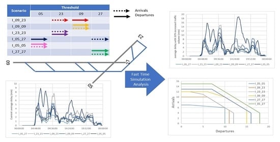
Having regard to the airside capacity (which takes into account runways, taxiways, aircraft stand taxi lanes, apron taxiways, and aircraft stands), the technical capacity value is the maximum number of aircraft movements that can be managed in a unit of time over a peak period, having regard to the adopted procedures, traffic rules, and an acceptable average delay that reflects the quality of service (Figure 1 presents a technical capacity curve for a 10-min delay threshold).
The declared capacity is the number of movements that can be processed in one hour. It is a fixed value provided by each airport manager. This value reveals a strategic choice made by the airport manager: the declaration of a much lower capacity than the optimal one allows reducing the possible delays until the weather conditions are unfavorable, but the number of hourly movements that can be performed is smaller.
The present study aims to calculate the technical capacity of an airport whose infrastructure layout has two crossing runways. Six scenarios have been considered: each one refers to the busiest volume in the reference year under different weather conditions. The current number of managed movements has been increased, with 10% steps up to double it. Therefore, 10 clones have been examined for each starting scenario (one clone to each 10% increase). Once the various clones have been simulated, output data have been extrapolated in terms of occupancy, delay, and taxiing time in order to determine the airside capacity for each of them. The results from different scenarios have allowed the identification of the best performing configuration.
2. Methods
Different methods allow calculating airport capacity: they differ in terms of effort, data requirements, and costs [10]. ACRP [6] distinguishes 5 types of airport capacity assessment tools:
- Level 1: the capacity performances depend on the runway layout and the fleet mix composition. An example of this level is provided by FAA AC 150/5060-5 [4]: it provides the maximum hourly capacity values and an annual capacity of the analyzed system, modeling it as a predefined layout that fits as well as possible the examined airport;
- Level 2: charts, nomograms, and spreadsheets consider the airport layout (i.e., taxiways and gates), the fleet mix composition, the percentage of arrivals to total operations, and the percentage of touch and go operations. Chapter 3 of FAA AC 150/5060-5 reports an example of this method [4];
- Level 3: analytical models consider the final speed of approaching aircraft, separations, and ATC rules. Capacity values are relatively easy to calculate, but they overlook the airside layout and the airspace characteristics. Chapter 5 of [4] reports an example of this approach;
- Level 4: simulation models consider both input data of Level 3 and factors, such as the geometry of arrival and departure routes or fleet mix on each runway;
- Level 5: aircraft delay simulation models (e.g., fast time simulation or real-time models) are the most advanced tool to study the whole airport: they cover all aspects of the airport, not only the airside-related ones, reconstructing the overall gate-to-gate environment. The output data contain data on capacity and delays, curves of noise, engine-on waiting time, fuel consumption, environmental impacts, and workload of air traffic controllers. These methods have been studied for several years, and, currently, there are some very sophisticated software products [15,16] that can give results very close to reality when the configuration of the infrastructure is complex or an advanced design level is required [8,10,17,18,19,20,21,22]. Level 5-models can incorporate a wide range of features (e.g., complete airport layouts, ATC procedures, airport operating procedures, runway entry and exit points and taxiways routes, fleet mix, wake turbulence classification, separation over time, turnaround times, and control tower activities) [11,18]. The output data contain data on capacity and delays, curves of noise, engine-on waiting time, fuel consumption, environmental impacts, and workload of air traffic controllers [11].
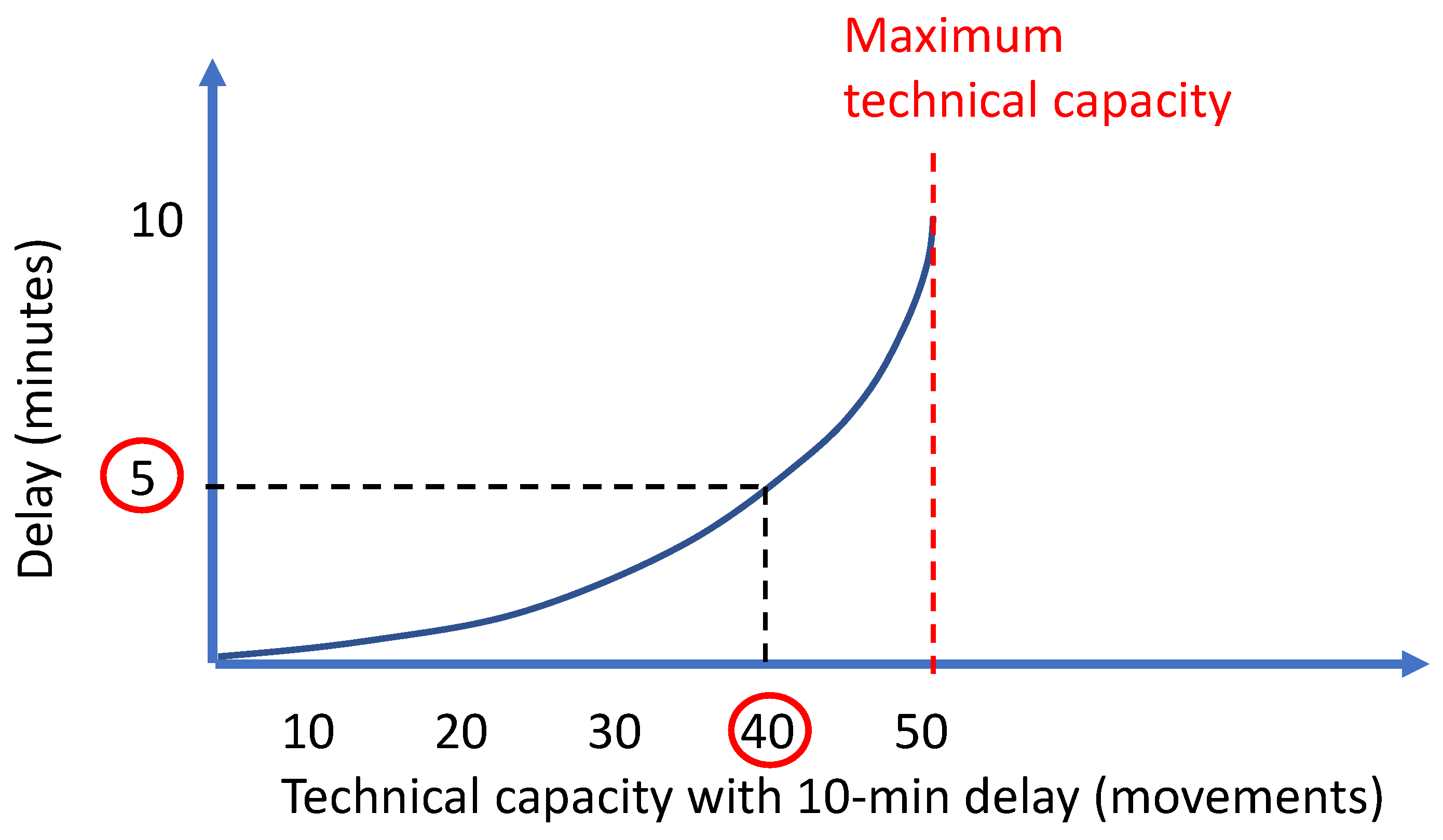
In this study, a fast time simulation (FTS) model has been built to calculate the capacity of an international airport whose layout is composed of a two-runway system, with two dependent, not perpendicular runways (i.e., RWY 09/27 and RWY 05/23) (Figure 2). The used software is AirTOp (Air Traffic Optimization), a gate-to-gate fast time simulator [16]. The simulation model is a simplified and virtual replica of a real system: given required levels of precision and detail, it reflects the set of relevant geometrical and procedural characteristics. The algorithms in the platform allow realistic simulations by creating airport models and air spaces in a 3D environment that changes over time and can be configured by setting a series of input variables. The analyses are faster than reality: depending on the number of input data, the software can take a few seconds or minutes to simulate one day of real-time. In the implemented model, all geometrical input data comply with the Aeronautical Information Publication of the airport: they consider runways, taxiways, rapid exit taxiways, aprons, and holding bays; moreover, this source has been considered to implement in the simulation all the adopted airside and ground side procedures (e.g., self-maneuvering or push-back procedures on the apron, standard instrument departure, and standard terminal arrival route for departures and arrivals, respectively).
In 2019, almost 45,000 movements (90% performed by A319 and A320) and more than 7,000,000 passengers were registered in this airport. The volume of movements strongly depends on the month and the day of the week: the number of movements during the busiest month (i.e., August) differs by more than 30% from that of the less-trafficked one (i.e., March); during the busiest month, the number of daily movements ranges between 145 and 186. Statistical anomalies of traffic volume in the busiest month (e.g., days with unfavorable weather conditions, closure of airside infrastructure, irregular occurrences, and errors in air traffic management systems) have been ignored in order to identify the statistically significant value of daily movement. Table 1 lists the input data about weather conditions.
Under such conditions, the value of the occurred daily movements nearest to the statistical average value has been 178. Wake turbulence (WT) and size category of the airplanes composing the fleet mix have been analyzed in order to consider their negative effects on throughput (e.g., on-air longitudinal separation and on-ground constraints). Indeed, a homogeneous traffic fleet leads to higher throughput and a standard minimum separation equal to 3 NM. On the other hand, when the fleet mix is mixed (e.g., variable VT category [4,23]), the airplane on-air longitudinal separation is up to 8 NM if a light aircraft follows a super heavy one. In this study, the mixed fleet mix has required the definition of a variable airplane on-air longitudinal separation during simulations. Particularly, for each movement that occurred during this day, the FTS simulations have considered origin/destination, route, aircraft type, airline, flight number, and arrival/departure time.
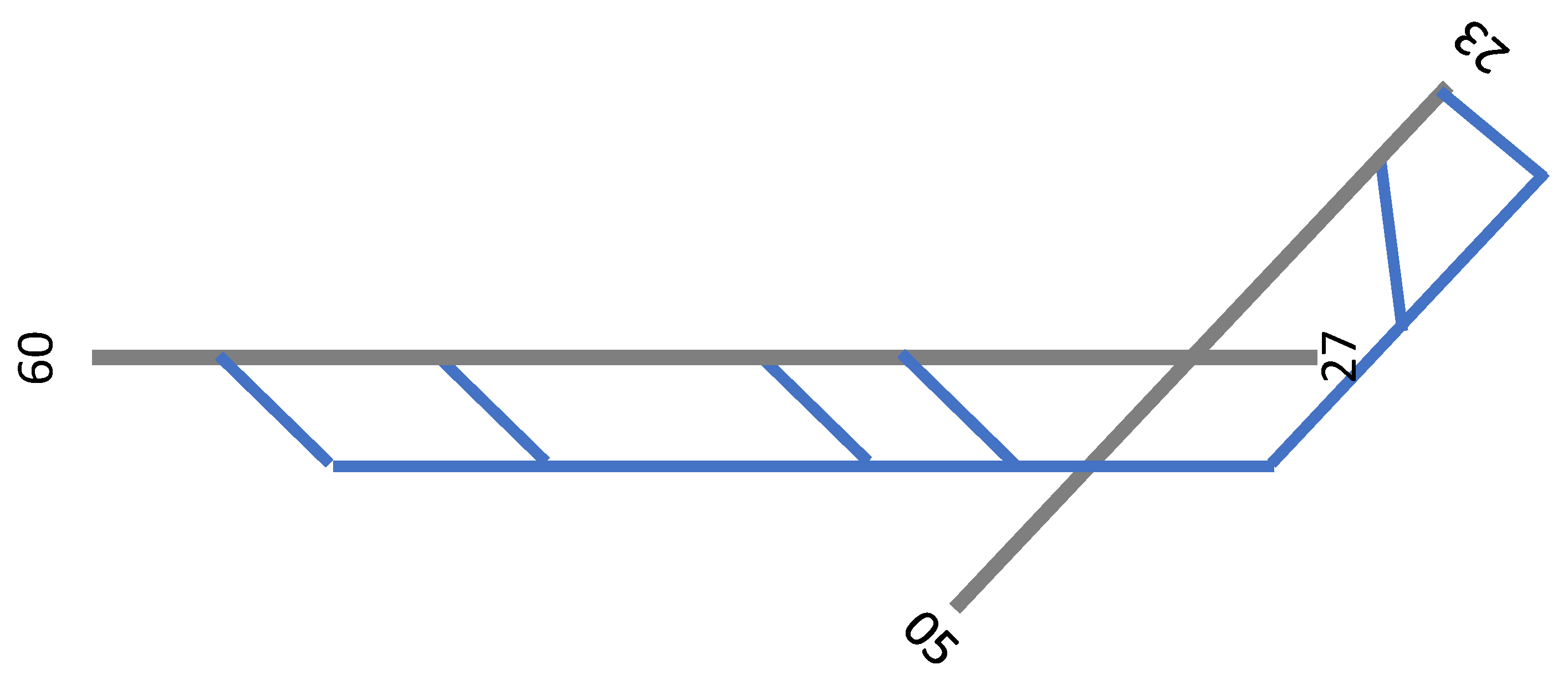
The baseline scenario (i.e., traffic volume and composition in the busiest day) (BS) and six operative scenarios with increased traffic volume have been analyzed: they differ for runway use under different wind conditions (in Figure 3, departures are represented by continuous arrows, arrivals by dotted arrows):
- Scenario 05_27 (I_05_27): departures from threshold 05 and arrivals on threshold 27 (blue arrows in Figure 3);
- Scenario 09_23 (I_09_23): departures from threshold 09 and arrivals on threshold 23 (red arrows in Figure 3);
- Scenario 27_27 (I_27_27): both departures and arrivals in threshold 27 (green arrows in Figure 3);
- Scenario 09_09 (I_09_09): both departures and arrivals in threshold 09 (orange arrows in Figure 3);
- Scenario 23_23 (I_23_23): both departures and arrivals in threshold 23 (purple arrows in Figure 3);
- Scenario 05_05 (I_05_05): both departures and arrivals in threshold 05 (pink arrows in Figure 3).
The traffic volume of BS has been increased with 10% steps up to double BS. Therefore, 10 clones (CLs) have been examined for each increased scenario (one clone to each 10% increase). The FTS simulation has allowed to model and simulate separately all the examined cases in order to identify their performances and weaknesses. Particularly, for each CL, 10 runs have been calculated in order to minimize randomness in the obtained results.
Data reports are automatically organized into 10-min buckets and rolling hours: for each period, the total delay (i.e., both approaching delay and on-ground delay) and the hourly activity (i.e., both arrivals and departures) have been considered. For each increased scenario, two graphs are produced:
- the former presents delays. Particularly, each delay value is the average of ten delay values obtained from 10 runs carried out for each clone. This representation allows verifying if the average delay overcomes the average delay threshold (i.e., 10 min);
- the latter presents the daily throughput in a Cartesian plane. Given an average delay for a single aircraft of less than 10 min, each point represents the number of operations that can be performed in one hour without violating air traffic control rules, assuming continuous aircraft demand.
The Pareto frontier (i.e., the set of pairs of arrivals and departures at which both the arrival and the departure rate cannot be simultaneously increased) identifies the saturation capacity of the airport. Firstly, the study has identified the maximum throughput at the balanced priority (i.e., the maximum admitted movements on the 45-degree line) and then verified that other points on the frontier ensure the maximum throughput within the admitted delay.
3. Results
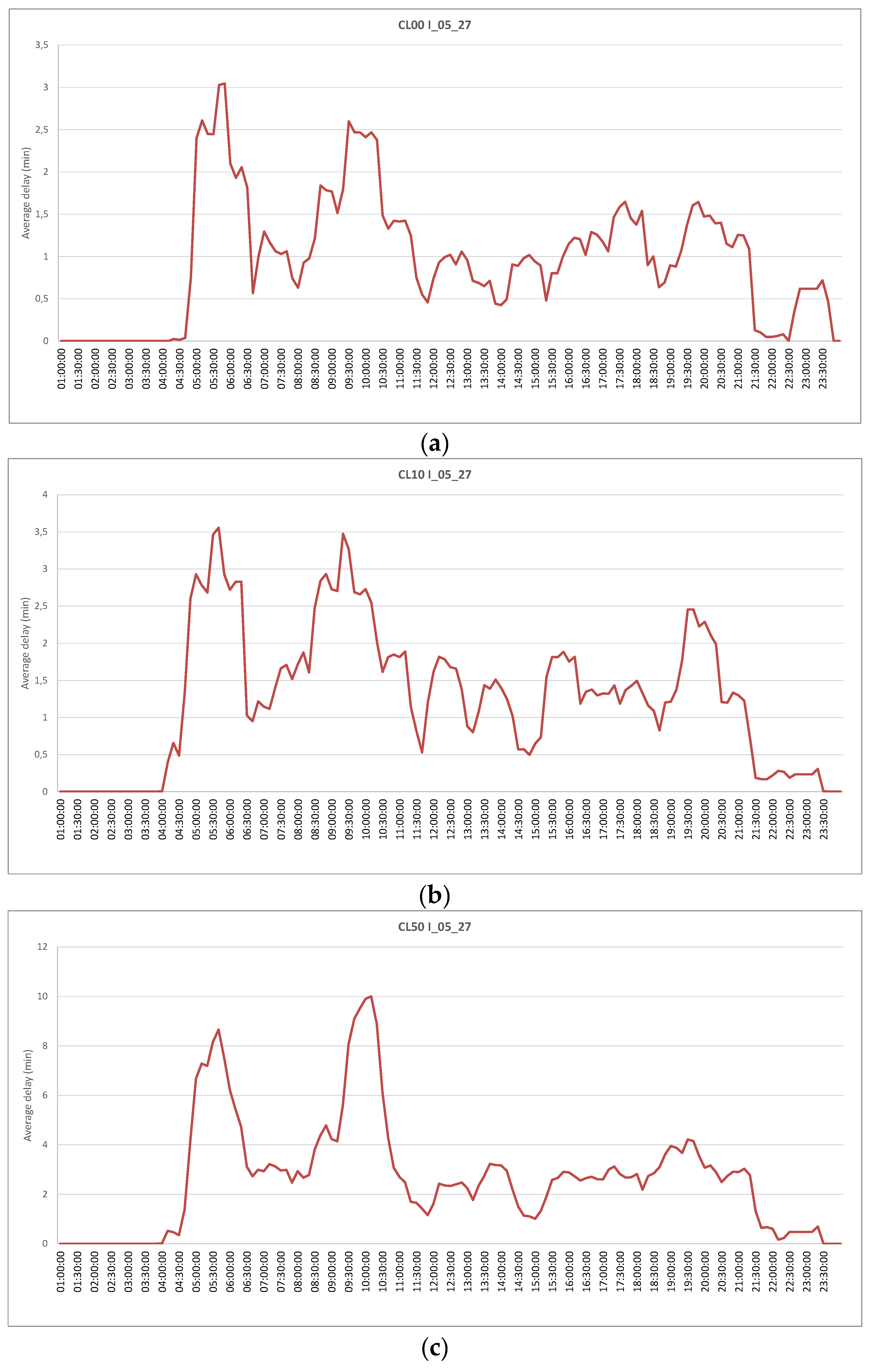
The simultaneous study of the delay report and the Pareto frontier has permitted to evaluate the saturation of the examined airport having regard to its throughput. For each examined scenario, the average hourly delay and the number of movements have been considered: the average delay is calculated considering the sum runs of each clone; when its value reaches or exceeds 10 min, the run is considered. The throughput representation refers to all 10 runs for each clone: it allows studying the daily trend of movements. Figure 4, Figure 5 and Figure 6 represent the results for I_05_27: average delay, throughput, and Pareto frontier, respectively.
In Figure 4, the average delay for I_05_27 CL00 (current traffic volume) is below the limit (i.e., 10 min) (Figure 4a); with CL10, the average delay has increased, but it is below the limit (Figure 4b); CL50 is the first examined clone where average delays coincide with the limit (Figure 4a): it is the last step of increased traffic not overcoming the average delay threshold. Therefore, in Figure 4, the authors have not presented the results from other clones.
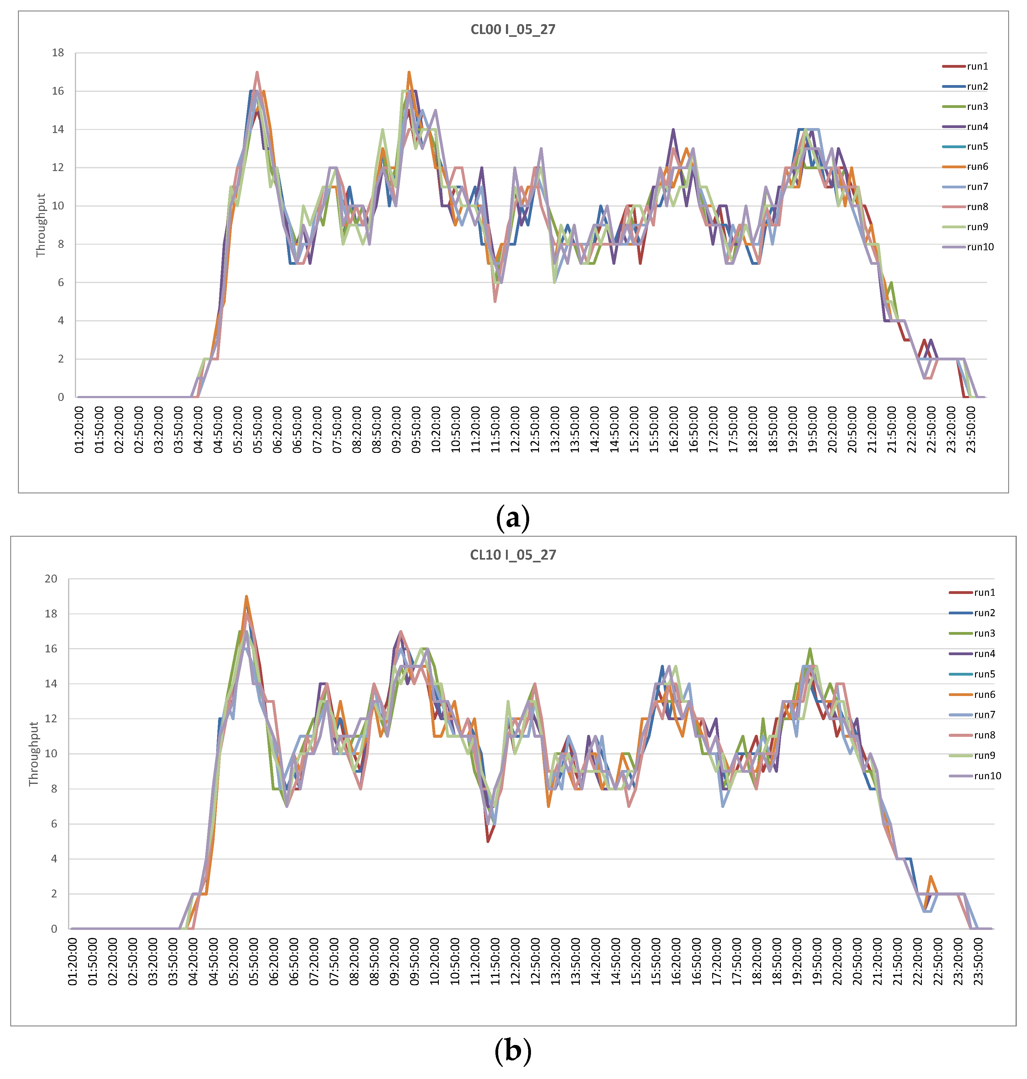
The results in Figure 5 highlight that peaks of hourly throughput correspond to peaks of average delay (Figure 4); for each clone, throughput in different runs is almost constant: during simulations, traffic jams or difficulty in the management of the demand have been absent. Moreover, throughput peaks are increasing with the clones (Figure 5a,b) until CL50 saturation conditions do not occur. Over CL50 (Figure 5c,d), the already achieved throughput peaks are almost constant: by increasing the airport traffic by over 50%, the current volume causes saturation of the infrastructure.
Figure 6 represents the envelope of the Pareto frontier (green line) obtained for I_05_27 clones from CL00 to CL50: the FTS software has increased by 50% the current arrival/departure mix to obtain that of CL50. In the balanced mode (i.e., on the main diagonal), the overall number of movements is 22 (11 departures and 11 arrivals), and it is the maximum throughput value that ensures a not more than 10 min delay. Once identified the maximum balanced throughput, it is taken as a reference for identifying other points on the frontier, varying the number of movements, and having delay values under the established threshold. Therefore, points obtained for clones with more than 50% traffic increase are not represented because they refer to average delay values over 10 min.
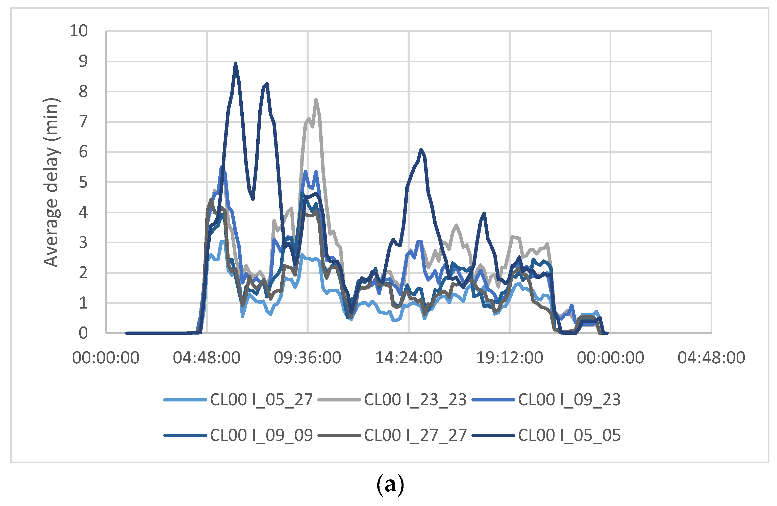
The presented output have been considered for all the examined scenarios. Figure 7a,b represent the comparison of average delay for CL00 and CL30, respectively.
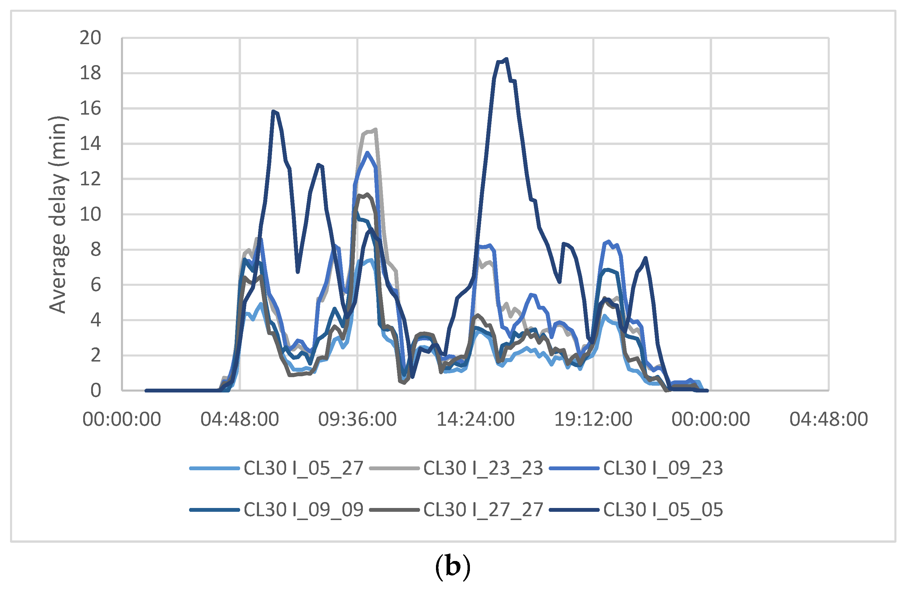
In Figure 7a, all delay values are below the limit threshold: on average, the lowest average one is in I_05_27. This result is related to the runway layout: RWY 27, where arrivals are scheduled, crosses in its initial part RWY 05, where departures are scheduled. This allows departures to leave immediately after the landing of the arriving aircraft. Scenarios I_09_09 and I_27_27 have the average delay curve similar to that of I_05_27: it is consistent because they are the same physical runway, but different thresholds are considered. Delays of I_09_09 and I_27_27 are greater than I_05_27 because of the runway’s layout: it is necessary to wait for the arriving aircraft to cover the entire runway before being able to free it. I_ 09_23 crosses RWY 23, where the arrivals are expected: this means that a departing aircraft on RWY 09 should wait for the arriving aircraft on RWY 23 to clear at least half runway: such conditions justify the high average delay values. Finally, I_05_05 and I_23_23 give the worst performance because of double crossings. With the same traffic increase (30%), the I_05_05 configuration has the highest delay (i.e., more than 18 min) and does not satisfy the 10-min limit threshold at different times of the day. Therefore, a traffic increase of 30% is not sustainable for I_05_05; the same is for I_23_23 (maximum average delay 15 min). The scenario that best supports this increase in terms of delays is I_05_27 (maximum average delay almost equal to that of CL_00). I_27_27 and I_09_09 tend to remain below the limit threshold (maximum average delay of 11 min and 10.5 min, respectively). However, I_09_09 has a slightly lower average delay (i.e., 10.5 min) than I_27_27 as the arrivals can take the quick exits on the runway, leaving the runway free faster than I_27_27. Finally, I_09_23 has a maximum average delay (13 min), higher than the other critical scenarios I_05_05, I_27_27, and I_09_09.
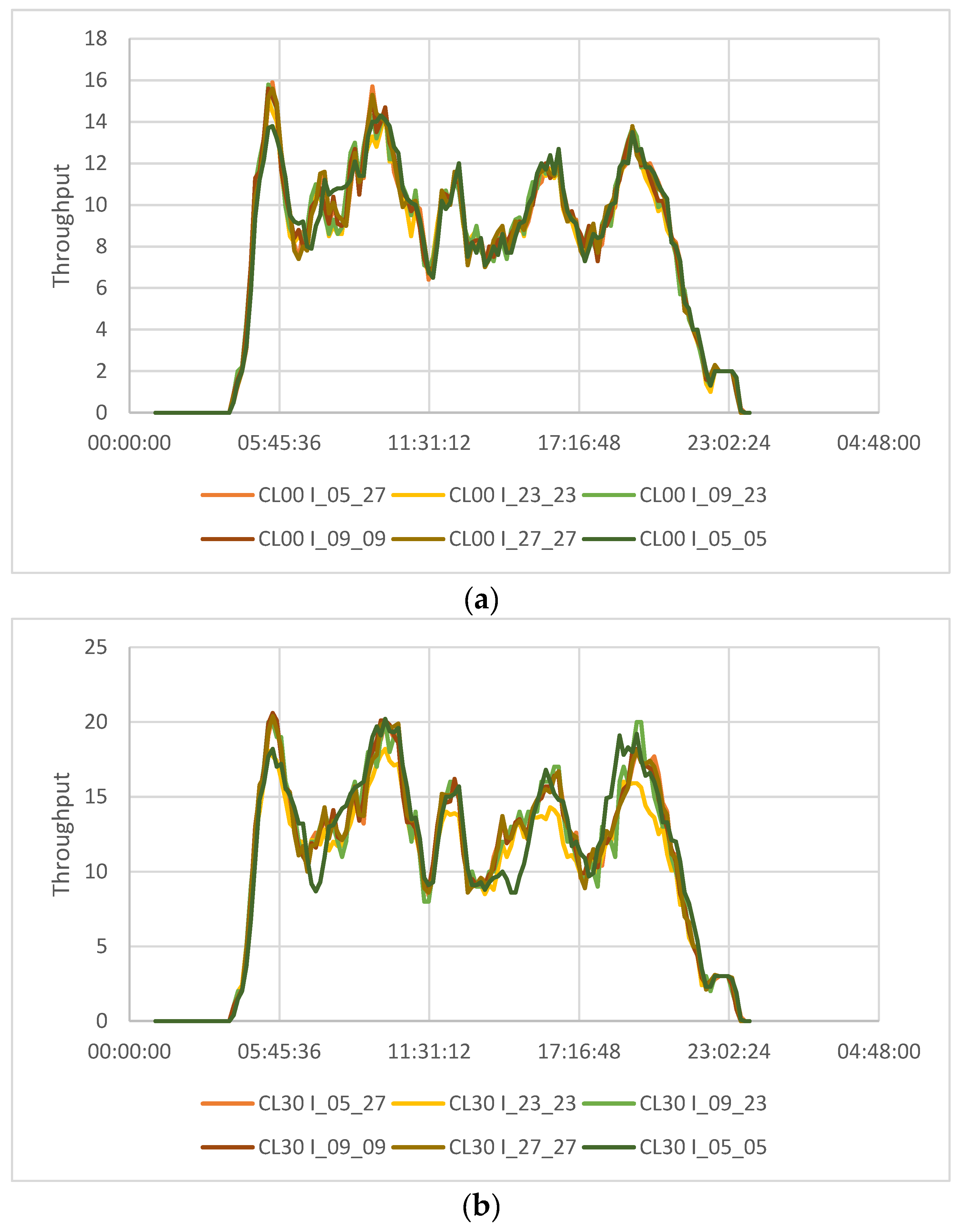
In all the examined scenarios, the highest delays are during morning hours, but important differences are in terms of throughput of CL00 and CL30 (Figure 8a,b, respectively).
In Figure 8a, all scenarios have the same throughput trend: CL_00 does not report increases, and, consequently, it is expected that the behavior of each scenario is almost similar. Only scenarios I_05_05 and I_23_23 deviate from other throughput curves because they cannot support the same number of movements of others. It requires moving some movements to the following time slots with a consequent increase in delays and deviation of the movement curves compared to the standard trend. The other four scenarios could efficiently manage the movements even after the 30% increase.
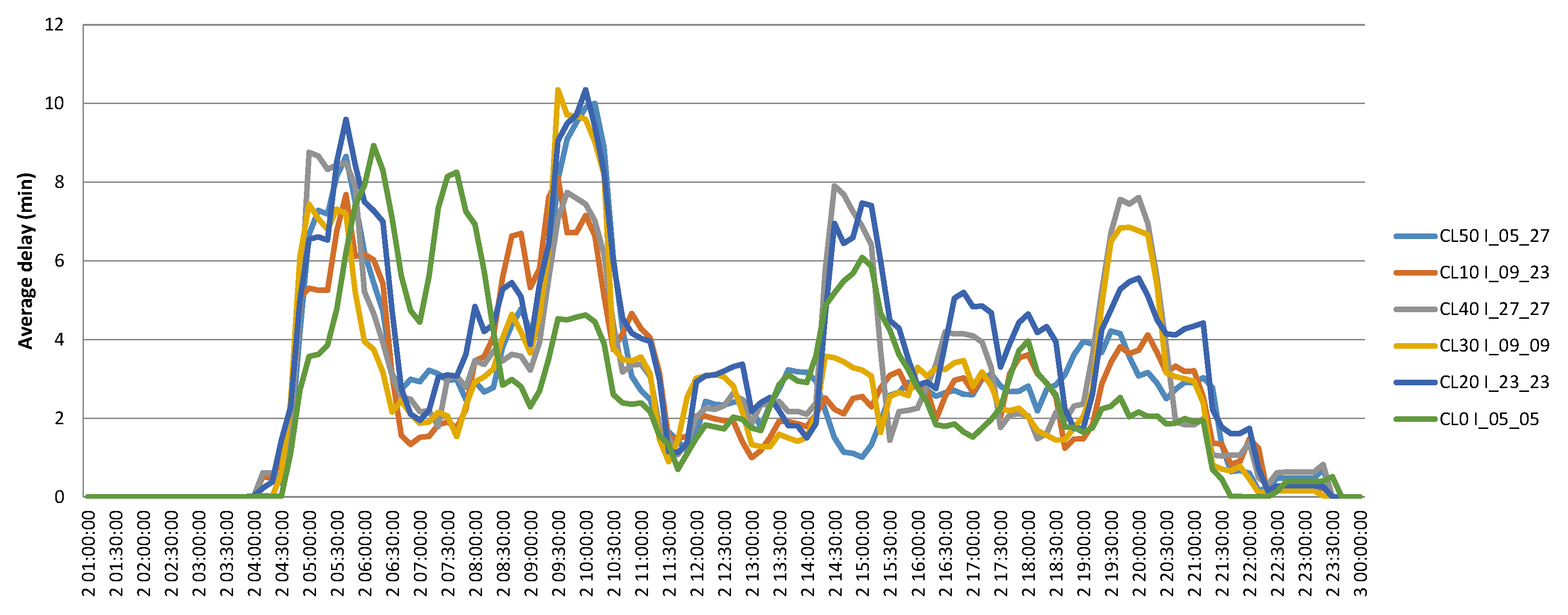
Finally, the authors have compared values of delays and movements obtained for saturation clones of each scenario (Figure 9).
The clones that cause saturation on each scenario are different: CL50 for I_05_27, CL10 for I_09_23, CL40 for I_27_27, CL30 for I_09_09, CL20 for I_23_23, and CL00 for I_05_05. Therefore, the most performing scenarios are I_05_27, I_27_27, and I_09_09 because they have higher percentages of traffic increase within the threshold delay limit. Among these, I_05_27 has the lowest delay and the highest increase, but it is a mixed configuration and has the disadvantage of runway crossing. Particularly, for I_27_27, it is possible to reach a higher increase compared to I_09_09, but it involves a greater delay. The choice of the most advantageous scenario between them depends on a strategic decision: the airport manager will opt for I_27_27 if he prefers having more traffic; on the other hand, he will opt for I_09_09 if he prefers having lower delay values. I_09_23 has rather low delays, but the maximum traffic increase value is equal to 10%: a limited number of movements can be accepted in order not to exceed the delay. Due to runway crossing, both I_05_05 and I_23_23 have quite high delays and rather limited traffic increases.
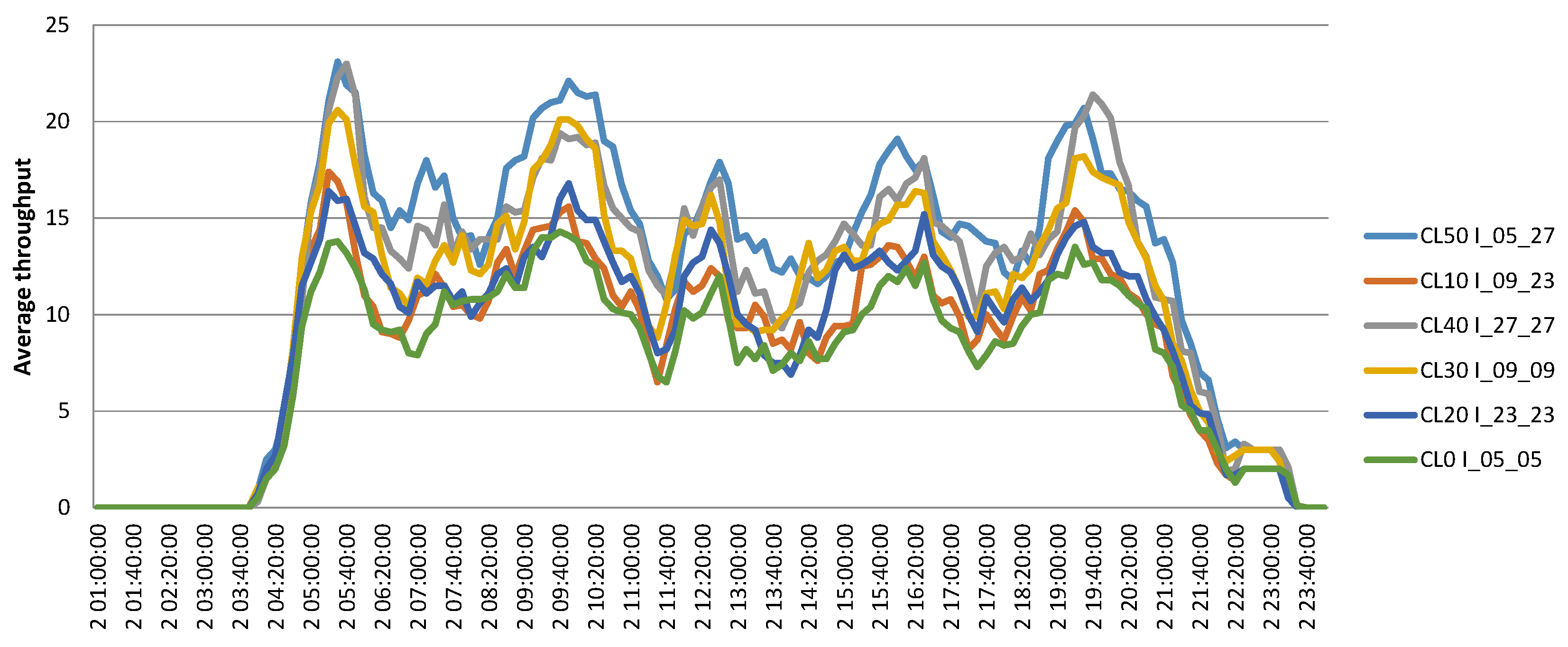
Having regard to the average results obtained for the saturation clone of each scenario, Figure 10 compares the throughput output.
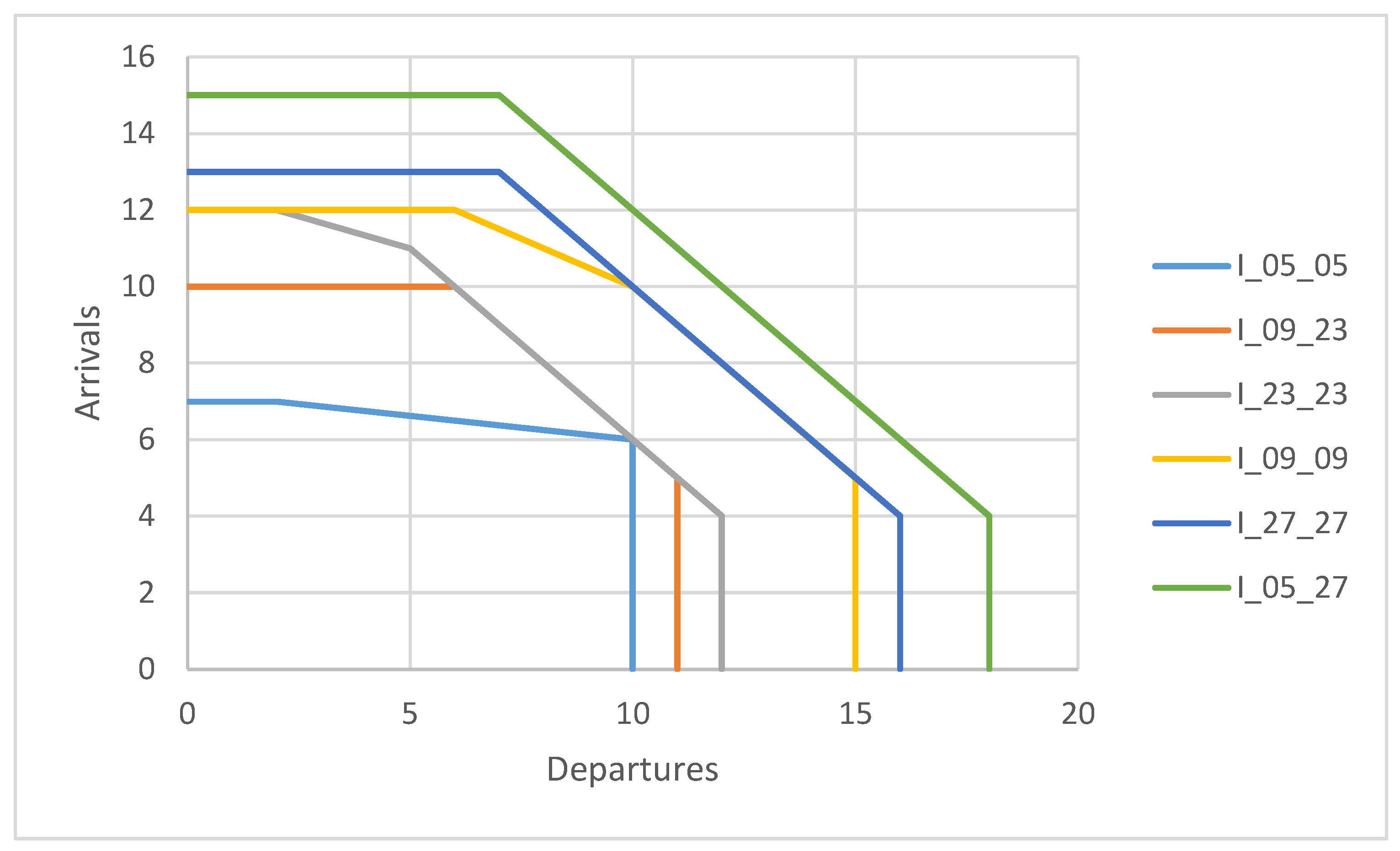
The throughput analysis highlights that I_05_27 has the highest number of hourly movements: it complies with the discussed data in Figure 9. Finally, the Pareto frontiers of the examined saturation scenarios are in Figure 11.
I_05_27 is the scenario that ensures the higher number of hourly movements (i.e., 22 with balanced conditions); both I_27_27 and I_09_09 allow 20 hourly movements with balanced conditions: they have a similar frontier. Both runway layout and aeronautical procedures affect the maximum hourly capacity of other scenarios: in balanced conditions, I_23_23, I_05_05, and I_09_23 have the same maximum number of allowable movements per hour (i.e., 16), but with decreasing performances in unbalanced conditions (when departures are given priority 12, 11, and 10, respectively; when arrivals are given priority 12, 10, and 7, respectively).
4. Conclusions
The airside capacity is the attitude to manage air traffic at take-off and landing movements with safety and within acceptable delays. It can be assessed with different five levels of analysis: simplistic and no longer updates methods attempt to describe real situations by approximating them to predefined configurations (levels 1 and 2); analytical capacity models (level 3) permit to analyze small size airports and some more information in inputs; most recent simulation techniques (levels 4 and 5) allow extremely detailed analyses.
In the present study, a fast time simulation model has been built to assess the airside capacity of an international airport whose layout is composed of two crossing runways. The obtained results, which depend on the input data (e.g., geometry, aeronautical procedures, ground handling processes, anemometric conditions, fleet mix composition), allow the airport manager to identify the most critical configurations in terms of delay and number of movements managed in 1 h having regard to the current traffic volume. Six scenarios have been considered: each one refers to the busiest volume in the reference year under different weather and usage conditions. On the other hand, the current number of managed movements has been increased with 10% steps up to double it in order to explore the technical or logistic feasibility of grown traffic. The most performing configurations are I_05_27 (22 movements/hour), I_09_09 (20 movements/hour), and I_27_27 (20 movements/hour). However, I_05_27 is less preferable than the others because it has an intersection between runways that slows down the airplane path fluidity. Therefore, it allows a possible increase in traffic and a lower delay value, but it cannot be considered the most performing because movements are less fluid than I_09_09 and I_27_27.
Author Contributions
Conceptualization, P.D.M. and L.M.; methodology, P.D.M.; software, L.M.; validation, L.M. and P.D.M.; formal analysis, L.M.; investigation, L.M.; data curation, P.D.M. and L.M.; writing—original draft preparation, L.M.; review and editing, P.DM. and L.M.; supervision, P.D.M. All authors have read and agreed to the published version of the manuscript.
Funding
This research received no external funding.
Acknowledgments
The authors sincerely thank Eng. Martina Possanzini for her support in building the FTS model and Italian air navigation service provider (ENAV) for having granted the use of the software AirTOp.
Conflicts of Interest
The authors declare no conflict of interest.
References
- International Civil Aviation Organization (ICAO). Advanced Surface Movement Guidance and Control Systems (A-SMGCS) Manual. Doc 9830 AN/452, First Edition. Available online: https://www.icao.int/Meetings/anconf12/Document%20Archive/9830_cons_en[1].pdf (accessed on 9 October 2020).
- International Civil Aviation Organization (ICAO). Manual on Global Performance of the Air Navigation System. Doc 9883, First Edition. Available online: http://www.aviationchief.com/uploads/9/2/0/9/92098238/icao_doc_9883_-_manual_on_global_performance_of_air_navigation_system_-_1st_edition_-_2010.pdf (accessed on 9 October 2020).
- Airports Council International (ACI). Guide to Airport Performance Measures; ACI World: Montreal, QC, Canada, 2012. [Google Scholar]
- FAA. Airport Capacity and Delay; AC 150/5060-5; APP-400, Office of Airport Planning & Programming, Planning & Environmental Division: Washington, DC, USA, 1983.
- ACRP. Evaluating Airfield Capacity; Report 079; Transportation Research Board: Washington, DC, USA, 2012. [Google Scholar]
- ACRP. Defining and Measuring Aircraft Delay and Airport Capacity Thresholds; Report 104; Transportation Research Board: Washington, DC, USA, 2014. [Google Scholar]
- Eurocontrol. Airport Capacity Methodology Assessment. ACAM Manual, v.1.1. 2016. Available online: https://www.eurocontrol.int/sites/default/files/publication/files/nom-apt-acap-acamman-v1-1.pdf (accessed on 9 October 2020).
- Di Mascio, P.; Cervelli, D.; Comoda Correra, A.; Frasacco, L.; Luciano, E.; Moretti, L.; Nichele, S. A Critical Comparison of Airport Capacity Studies. J. Airpt. Manag. 2020, 21, 307–321. [Google Scholar]
- Horonjeff, R.; McKelvey, F.; Sproule, W.J.; Young, S.B. Planning & Design of Airports, 5th ed.; Mc Graw Hill: New York, NY, USA, 2010. [Google Scholar]
- Di Mascio, P.; Cervelli, D.; Comoda Correra, A.; Frasacco, L.; Luciano, E.; Moretti, L. Effects of Departure MANager (DMAN) and Arrival MANager (AMAN) Systems on Airport Capacity. J. Airpt Manag. 2020. accepted paper. [Google Scholar]
- Di Mascio, P.; Carrara, R.; Frasacco, L.; Luciano, E.; Moretti, L.; Ponziani, A. Influence of Tower Air Traffic Controller Workload and Airport Layout on Airport Capacity. J. Airpt. Manag. 2020. accepted paper. [Google Scholar]
- Moretti, L.; Cantisani, G.; Caro, S. Airport veer-off risk assessment: An italian case study. ARPN J. Eng. Appl. Sci. 2017, 12, 900–912. [Google Scholar]
- Di Mascio, P.; Loprencipe, G. Risk analysis in the surrounding areas of one-runway airports: A methodology to preliminary calculus of PSZs dimensions. ARPN J. Eng. Appl. Sciences 2016, 11, 13641–13649. [Google Scholar]
- Di Mascio, P.; Perta, G.; Cantisani, G.; Loprencipe, G. The public safety zones around small and medium airports. Aerospace 2018, 5, 46. [Google Scholar] [CrossRef] [Green Version]
- FAA. Simmod Manual: How Simmod Work. 2010. Available online: http://www.tc.faa.gov/acb300/how_simmod_works.pdf (accessed on 22 August 2020).
- Airtopsoft. Airtopsoft Overview. Available online: http://airtopsoft.com (accessed on 22 August 2020).
- Ignaccolo, M. A Simulation Model for Airport Capacity and Delay Analysis. Transp. Plan. Technol. 2003, 26, 135–170. [Google Scholar] [CrossRef]
- Čokorilo, O. Human Factor Modelling for Fast-Time Simulations in Aviation. Aircr. Eng. Aerosp. Technol. 2013, 85, 389–405. [Google Scholar] [CrossRef]
- Di Mascio, P.; Rappoli, G.; Moretti, L. Analytical Method for Calculating Sustainable Airport Capacity. Sustainability 2020, 12, 9239. [Google Scholar] [CrossRef]
- Bubalo, B.; Daduna, J.R. Airport Capacity and Demand Calculations by Simulation—The Case of Berlin-Brandenburg International Airport. NETNOMICS Econ. Res. Electron. Netw. 2011, 12, 161–181. [Google Scholar] [CrossRef]
- Tee, Y.Y.; Zhong, Z.W. Modelling and Simulation Studies of the Runway Capacity of Changi Airport. Aeronaut. J. 2018, 122, 1022–1037. [Google Scholar] [CrossRef]
- Postorino, M.N.; Mantecchini, L.; Malandri, C.; Paganelli, F. A Methodological Framework to Evaluate the Impact of Disruptions on Airport Turnaround Operations: A Case Study. Case Stud. Transp. Policy 2020, 8, 429–439. [Google Scholar] [CrossRef]
- International Civil Aviation Organization (ICAO). Doc 8643—Aircraft Type Designators. Available online: https://www.icao.int/publications/DOC8643/Pages/default.aspx (accessed on 22 August 2020).
Figure 1.
Example of the technical capacity curve for a 10-min delay threshold.

Figure 2.
Airport layout.

Figure 3.
Operative airport layout.

Figure 4.
Average delay for I_05_27 (a) CL00; (b) CL10; (c) CL50.

Figure 5.
Throughput for I_05_27 (a) CL00; (b) CL10; (c) CL50; (d) CL100.


Figure 6.
The envelope of Pareto frontier for I_05_27 clones from CL00 to CL50.

Figure 7.
Comparison of the average delay for all the examined scenarios (a) CL00; (b) CL30.


Figure 8.
Comparison of throughput for all scenarios (a) CL00; (b) CL30.

Figure 9.
Comparison of saturation capacity average delay for each scenario.

Figure 10.
Comparison of saturation capacity throughput for each scenario.

Figure 11.
The Pareto frontier of the examined scenarios.


Table 1.
Input data of weather conditions.
| Air Temperature (°C) | Humidity (%) | Visibility (km) | Wind Speed (km/h) | Pressure (mb) | Rain (mm) | Gusts | |||
|---|---|---|---|---|---|---|---|---|---|
| Average | Minimum | Maximum | Average | Maximum | |||||
| 19 | 13 | 23 | 80 | 20 | 11 | 21 | 1016 | 0 | absent |
Publisher’s Note: MDPI stays neutral with regard to jurisdictional claims in published maps and institutional affiliations. |
© 2020 by the authors. Licensee MDPI, Basel, Switzerland. This article is an open access article distributed under the terms and conditions of the Creative Commons Attribution (CC BY) license (http://creativecommons.org/licenses/by/4.0/).
Share and Cite
MDPI and ACS Style
Mascio, P.D.; Moretti, L. Hourly Capacity of a Two Crossing Runway Airport. Infrastructures 2020, 5, 111. https://0-doi-org.brum.beds.ac.uk/10.3390/infrastructures5120111
AMA Style
Mascio PD, Moretti L. Hourly Capacity of a Two Crossing Runway Airport. Infrastructures. 2020; 5(12):111. https://0-doi-org.brum.beds.ac.uk/10.3390/infrastructures5120111
Chicago/Turabian StyleMascio, Paola Di, and Laura Moretti. 2020. "Hourly Capacity of a Two Crossing Runway Airport" Infrastructures 5, no. 12: 111. https://0-doi-org.brum.beds.ac.uk/10.3390/infrastructures5120111