Application of Ground Penetrating Radar to Estimate Subgrade Soil Density


School of Environmental, Civil, Agricultural, and Mechanical Engineering, College of Engineering The University of Georgia, Athens, GA 30602, USA
*
Author to whom correspondence should be addressed.
Infrastructures 2020, 5(2), 12; https://0-doi-org.brum.beds.ac.uk/10.3390/infrastructures5020012
Submission received: 30 December 2019
/
Revised: 16 January 2020
/
Accepted: 23 January 2020
/
Published: 27 January 2020
(This article belongs to the Special Issue Smart Cities and Infrastructures)
Abstract
:Ground penetrating radar (GPR) technology has been widely used in pavement assessment over the last decade. Assessing the subgrade condition and monitoring its temporal variation provide valuable information regarding changes associated with pavement deterioration, allowing for the beneficial prediction of future road maintenance. This paper presents a method to estimate the density and water content of prepared subgrade soils of highly plastic silt using a 2 GHz GPR scan system and a simple exponential model. A bulk density prediction model was developed based on electromagnetic mixing theory to back calculate subgrade soils density. The model developed determines the soil’s dielectric constant, considering dielectric and volumetric properties of the three major components of soil: air, water, and solid particles. A series of laboratory tests was conducted on six (6) soil samples at various density levels to validate the newly developed model. For validation purposes, sand cone and dynamic cone penetration (DCP) tests were performed and compared with the estimated soils strength from GPR data. The results show that the prediction of soils density and stiffness using nondestructive technology helps efficiently forecast not only pavement deterioration, but potential risks to the subsurface pavement structure with all the advances of time saving using air coupled GPR antenna mounted on a moving vehicle.
1. Introduction
The main function of the subgrade is to provide adequate support to the pavement structure. Therefore, the subgrade should possess enough stability under adverse climate and loading conditions. Subgrade soil and its properties are also important in the design of pavement structure.
Pavement structure deteriorates over time, and pavement condition surveys are conducted periodically. Assessment of road condition comprises of two steps. The initial step is the visual inspection to distinguish cracks’ areas and useful assessment by evaluating surface parameters such as roughness and skid resistance. Besides, a structural evaluation is performed to assess subsurface layers to check for decreased thickness, need of interlock between different layers, engendering of splits, and loss of subsurface materials (i.e., sinkholes) that may well be in advance [1]. The whole pavement system depends basically on the subgrade strength that provides support to the pavement layers and guarantees an effective distribution of loads along depth. Subsequently, keeping up a strong subgrade supporting system is key for a structurally-sound pavement structure.
GPR scanning systems’ productivity is so promising that it is expected that hundreds of miles of road networks can be inspected in a shorter time duration than when using traditional methods. This finding makes it possible to support the decision-making process and to address maintenance funds in the most sustainable and efficient way. In addition, the accuracy of the radar inspection is also strategic for identifying and planning the most effective rehabilitation and maintenance works. Finally, the methodology is also very useful in preventing the severe damage that is not yet visible on the top surface of the pavement [2]. Most of the GPR scanning systems are used to estimate pavement layers thicknesses. According to the mechanistic empirical pavement design guide [3], ground penetrating radar GPR surveys of existing pavements are a key assessment method for pavement rehabilitation design. Although primarily used for thickness determination, GPR scans are also used to identify defects (e.g., voids, sinkholes) within the pavement layers and beneath the pavement [4].
This study evaluates the pavement structure using electromagnetic (EM) waves as a useful asset management tool. For homogeneous layers, the speed of the EM waves is proportional to speed of light. The coefficient of proportionality is the inverse of the square root of the layer dielectric constant [2].
The primary material property obtained from GPR surveys is the dielectric constant. The dielectric constant, also known as the relative permittivity, of a homogeneous media relates the relative EM velocity in a material to the speed of light in free space [5]
where,
εr = (c/ν) 2,
- εr = dielectric constant,
- c = speed of light in free space of 3 × 10⁸ m/s,
- ν = EM velocity in the material.
According to the EM mixing theory, the dielectric constant of an asphalt mixture is a function of the dielectric and volumetric properties of its components, that is, air, asphalt binder, and aggregate, yielding a direct physical relation between the dielectric constant of an asphalt mixture and its density [6]. Consequently, if validated mathematical models between the asphalt mixture dielectric constant and its density can be developed [6]. As shown in Equations (2)–(4), these density models are developed based on three EM mixing models, namely the complex refractive index model (CRIM), the Rayleigh model, and the Bottcher model, respectively [7].
where,
| Gmb = the bulk specific gravity of asphalt mixture, | εHMA = the dielectric constant of asphalt mixture, |
| Gmm= maximum specific gravity of asphalt mixture, | εb = the dielectric constant of binder, |
| Gsb = the bulk specific gravity of aggregate, | εs = the dielectric constant of aggregate |
| Gb = the specific gravity of binder, | Pb = the binder content, |
Note that in these equations, the specific gravity of a material is equal to the density of the material divided by the density of water at 4 °C (1 g/cm3), and therefore is numerically the same as the density of the material in g/cm3 [6].
2. Research Approach
The density of soil depends on the specific gravities and volumetric fractions of its components. Soil is a composite media that consists of voids, water, and solids. In a similar way the dielectric constant of the soil is a function of the dielectric and volumetric properties of its components. Various EM mixing models are available to predict the dielectric constant based of a mixture on the dielectric constants and volume fractions of its components.
In this study, mathematical models were developed to predict subgrade soil bulk specific gravity, which is equivalent to soil bulk density based on the dielectric constant using EM mixing formulae.
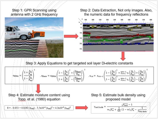
3. Data Acquisition and Processing
Laboratory and field equipment were used to build-up samples and record data for the analysis regarding this research as follows
3.1. Ground Penetrating Radar (GPR) System
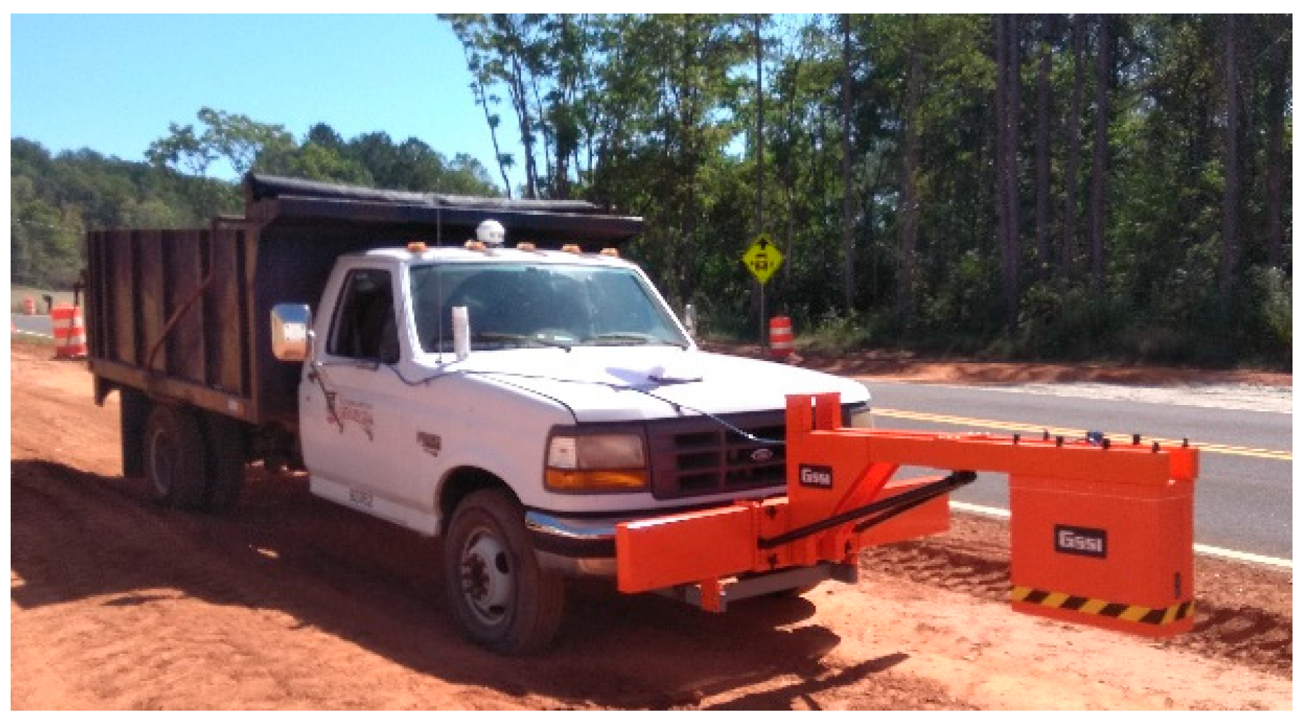
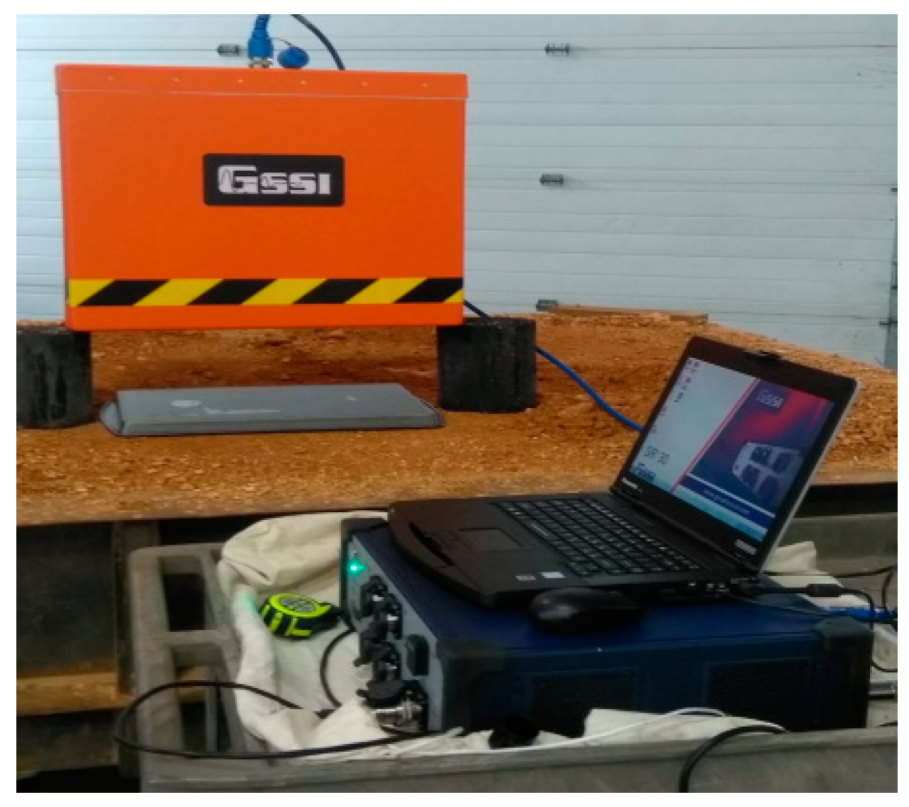
A 2 GHz air-coupled GPR antenna system is being used for this study. The GPR system was manufactured by Geophysical Survey Systems, Inc (GSSI). As depicted in Figure 1, the antenna was mounted in front of a truck, with the control unit set inside of the driving cabin. The global positioning system (GPS) device was used to precisely locate the data collected with the GPR longitudinally on the road. Figure 2 shows the data acquisition system to collect GPR and GPS data. The data acquisition system should be calibrated before each scan in order to validate the signals with a perfect reflection on a metal plate. In addition, this calibration provides some preliminary data for the data processing, with Am (amplitude of the reflected wave on the metal plate) to estimate the dielectric constants for the subsequent layers in order to calculate the density for the targeted layers by the GPR scan.
3.2. Samples Preparation
A problematic soil type readily found in North Georgia was used as the subgrade material. The soil index properties for these soils are provided in Table 1. The soil is classified as high plasticity silt (MH) per the Unified Soil Classification System (USCS) [8] or A-7-5 according to the American Association of State Highway and Transportation (AASHTO) classification system [9] or (SiH) according to the European Soil Classification System ESCS [10,11].
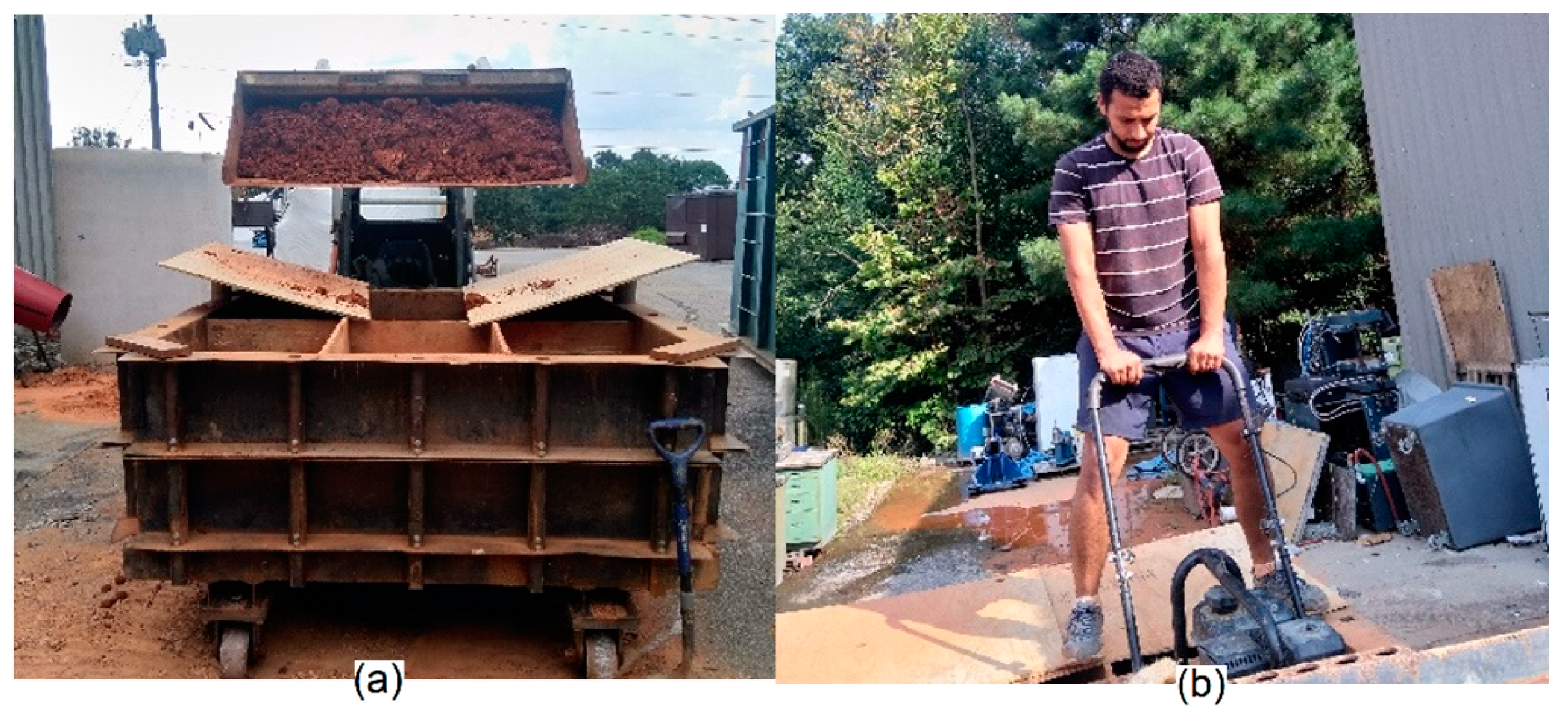
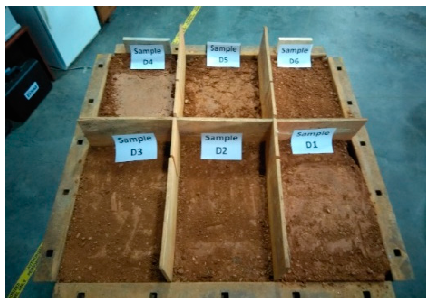
Test specimens were prepared in a large metal box measuring 1.8 m long × 1.8 m wide × 0.6 m deep (6 ft long × 6 ft wide × 2 ft deep), the box is divided to six sections as shown in Figure 3 and Figure 4. Each sample measures 0.9-m-long × 0.6 m wide. The soil was mixed with water till it reached the desired water content for soil compaction. The soil was then transported to the steel box and compacted using flat compactor as shown in Figure 3. Subgrade soil specimens were constructed with 0.3 m (12 in.) in depth and compacted to reach six (6) different density levels, as shown in Figure 4.
4. Data Analysis
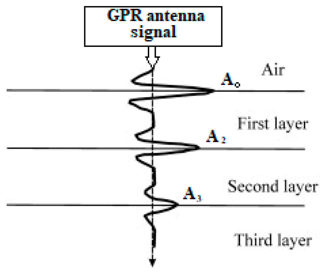
Figure 5 shows a schematic diagram of the reflections of a GPR signal from a layered pavement system.
4.1. Dielectric Constant(ε)
The dielectric constant is the ratio of the permittivity of a substance to the permittivity of free space. It is a dimensionless value and is also called relative permittivity. Permittivity is the measure of a material’s ability to store an electric field in the polarization of the medium. The dielectric constant is the ratio of capacity of a capacitor filled with dielectric material to the capacity of identical capacitor filled with air. It represents the ability of a material to store electrical energy in the presence of an electric field.
The dielectric values of the asphalt concrete and the base layers can be computed using the following Equations (5) and (6), respectively [12].
where
- εHMA = dielectric constant for the HMA layer,
- Ao = amplitude of the surface reflection, and
- Am = amplitude of the reflected signal collected over a metal plate placed on the surface.
- Abase = amplitude of the reflected signal collected over subbase layer surface.
The dielectric value εn for the third layer onwards (nth layer) can be evaluated as Equation (7):
γi is the reflection coefficient at the ith layer interface.
By far the most important factors in determining a soil’s dielectric permittivity are porosity and water saturation. Air has a relative permittivity of 1.0, whereas common soil-forming minerals have much higher relative permittivity. This means that for dry samples, the soil’s bulk dielectric permittivity decreases as the porosity increases [13].
4.2. Proposed Analytical Model
As mentioned earlier, it is concluded that soil bulk density, water content and porosity could be estimated based on the value of the dielectric constant.
Accordingly, a model is proposed through this research to estimate both mass water content and soil bulk density, using a dielectric constant calculated depending on field or lab measurements of GPR.
If Equation (2), which is made for asphalt concrete, is used for the soil medium with its different components, and using parameters of soil instead of Asphalt layer parameters as follows, Equation (9) can be written as
where,
| Gmb = γbulk = the bulk density of soil, | εHMA = εsoil = the dielectric constant of soil, |
| Gmm= γdmax = maximum dry density of soil, | εb = εw = the dielectric constant of water, |
| Gsb = GS = the bulk specific gravity of soil, | εs = εs = the dielectric constant of soil particles, |
| Gb = the specific gravity of binder =1, | Pb = w = water content, |
Topp et al. (1980) [14] proposed Equation (10) to estimate the volumetric water content (θ) in relation with dielectric constant of the soil. The water content of soil is calculated from volumetric water content as shown in Equation (11).
θ = −0.053 + 0.0292 (εsoil) − 5.5 × 10⁻⁴ (εsoil)2 + 4.3 × 10⁻⁶ (εsoil)3,
Relationship between gravimetric and volumetric water contents
Gravimetric water content (w) = mass of water/mass of dry soil = Mw/Ms
Volumetric water content (θ) = volume of water/volume of undisturbed soil = Vw/Vs
w * → Where (Soil Bulk Density)
w = θ/γsoil
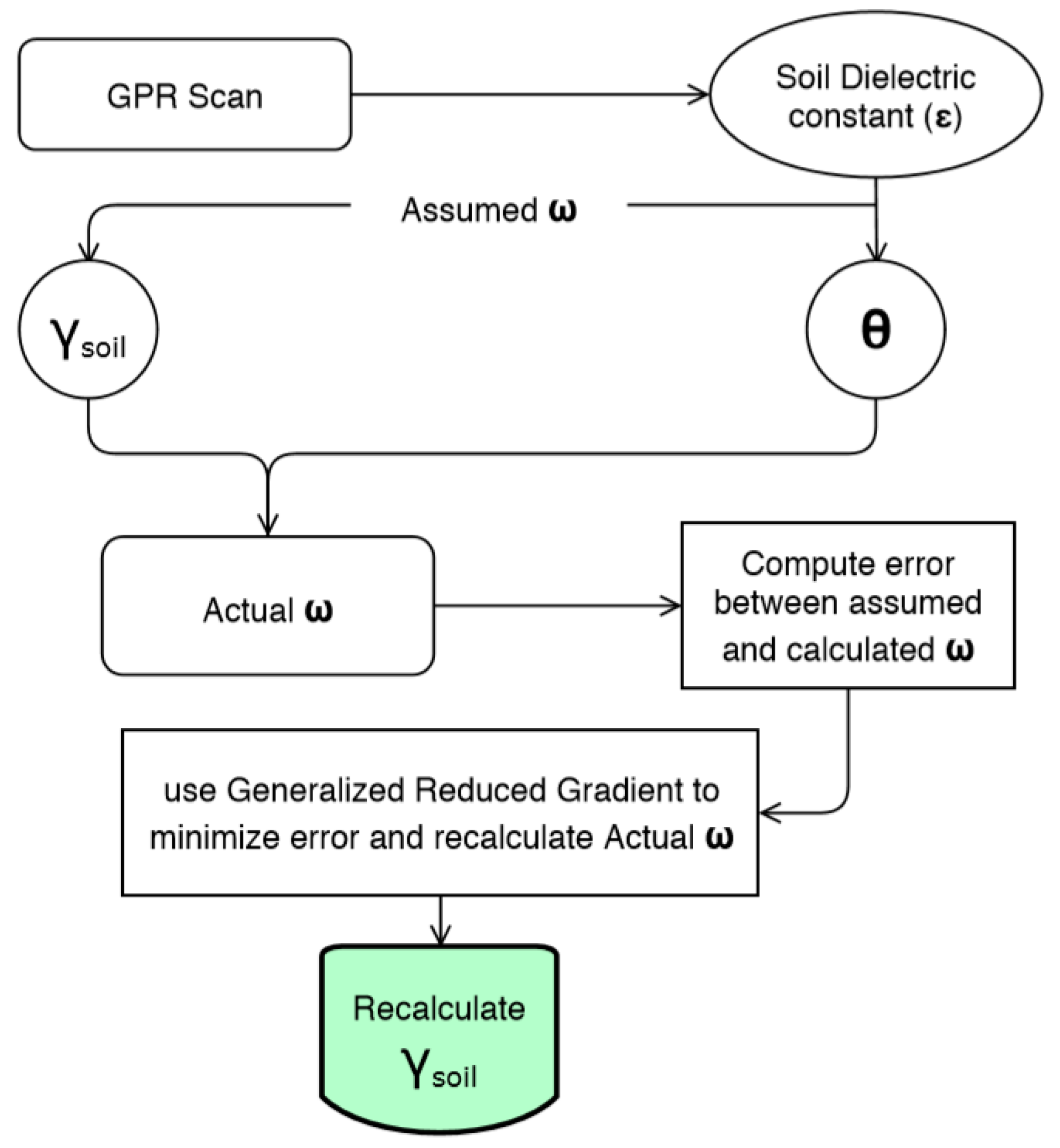
The soil bulk density is calculated using Equation (10) with an assumed gravimetric water content (w). Volumetric water content (θ) is calculated using Equation (11). It calculates the gravimetric water content (w), followed by the determination of error between the calculated and estimated gravimetric content. Generalized reduced gradient (GRG) was used to minimize the error and recalculate the correct values for estimated and calculated gravimetric water content, as shown in the flow chart in Figure 6.
5. Results
5.1. Soil Density
After the specimens were prepared, bulk density of each specimen was measured using sand cone tests. The results of sand cone tests are illustrated in Table 2.
5.2. GPR Data Collection
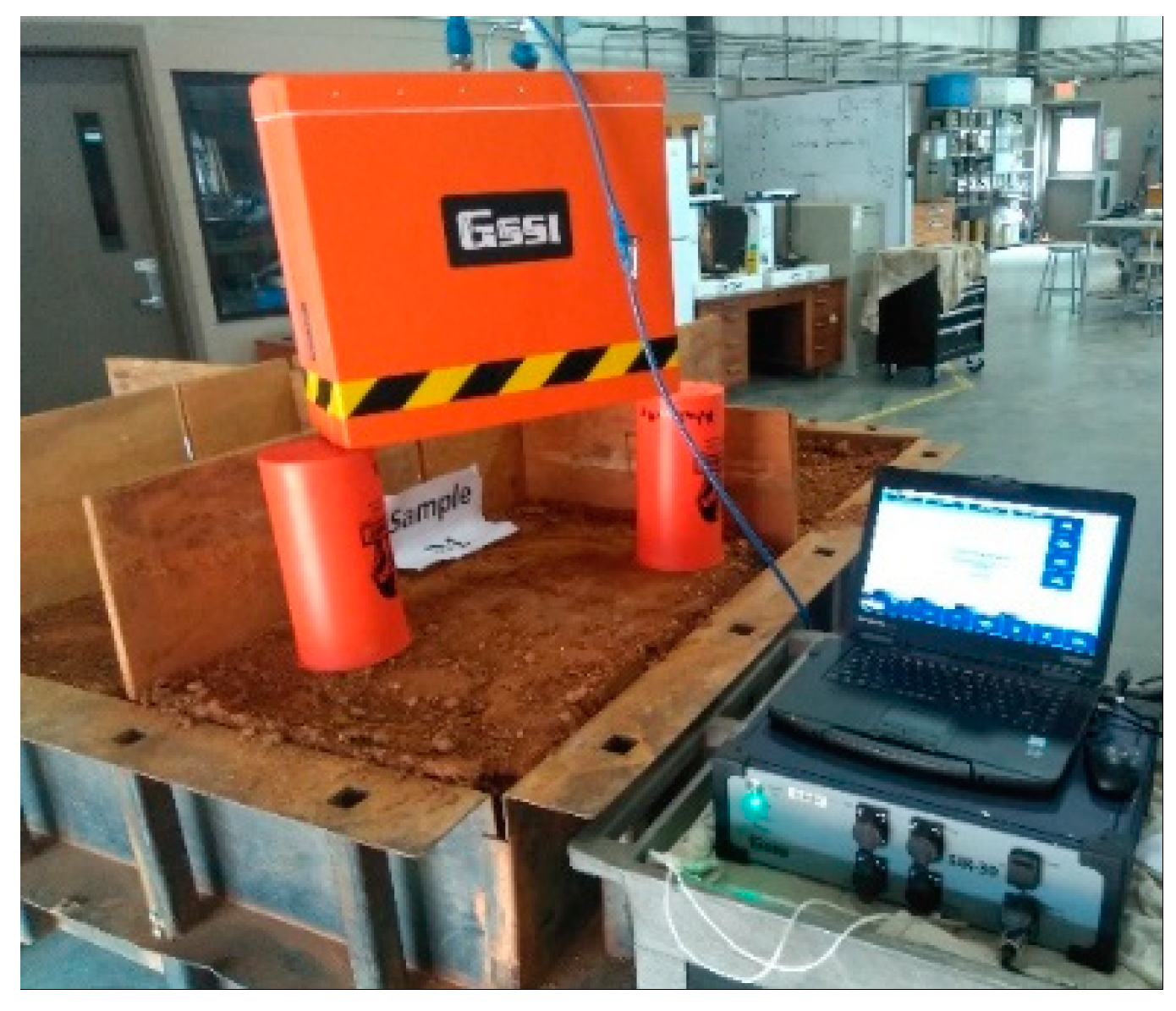
After sand cone tests were conducted, GPR data were collected from six (6) samples using a 2.0-GHz air-coupled antenna as shown in Figure 7.
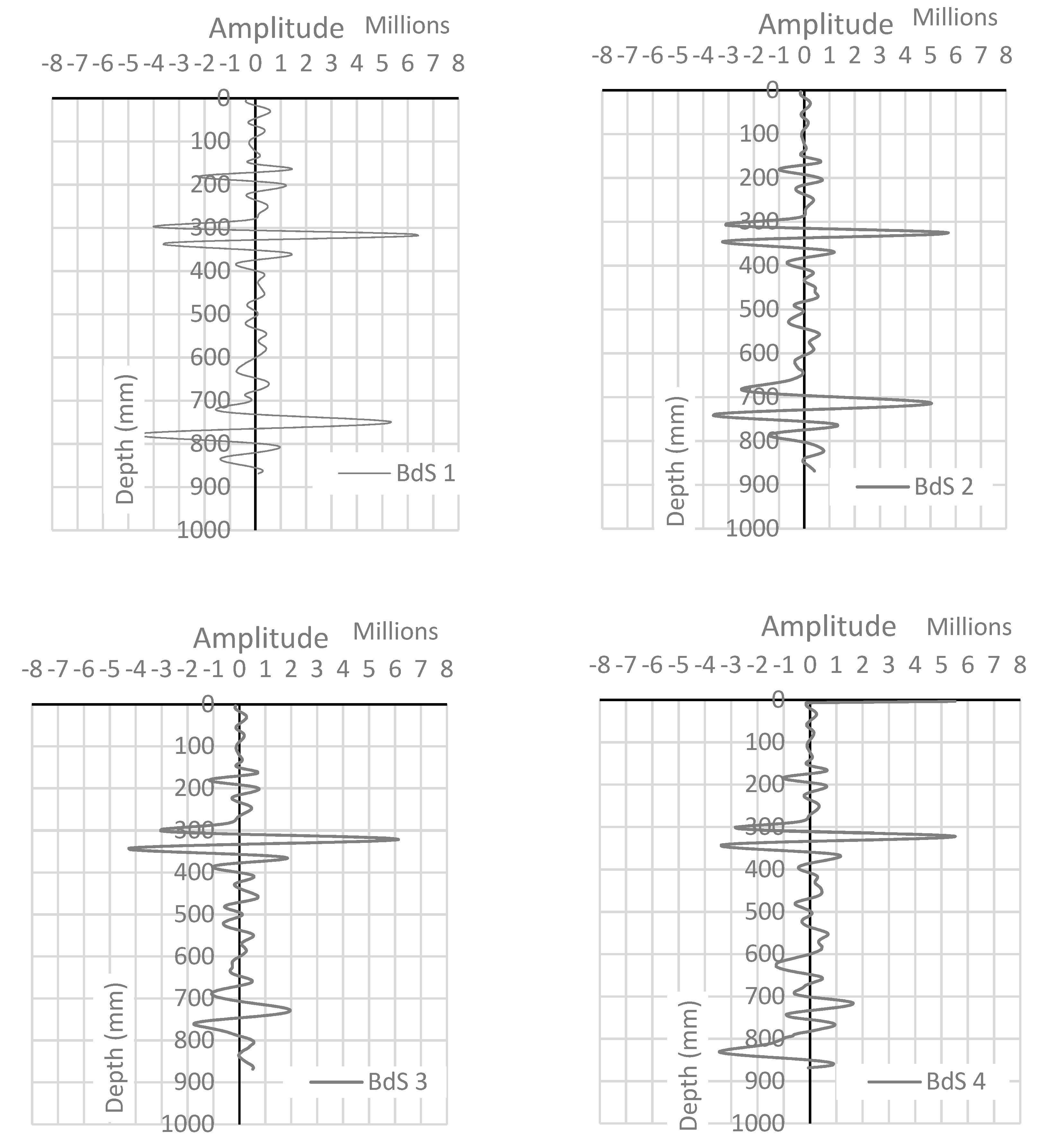
Figure 8 shows the amplitude of the surface reflection measured from each soil specimen using the GPR system. From the calibration process with a metal plate on top of soil specimen, Am was found to be 7,942,173. Using the measured amplitude values from GPR, dielectric constants for six (6) soil specimens were calculated using Equation (5). Table 3 summarizes the dielectric constant calculated for each specimen.
Based on Equations (9)–(11), soils bulk density and water content were calculated as illustrated in Table 4.
6. Analysis
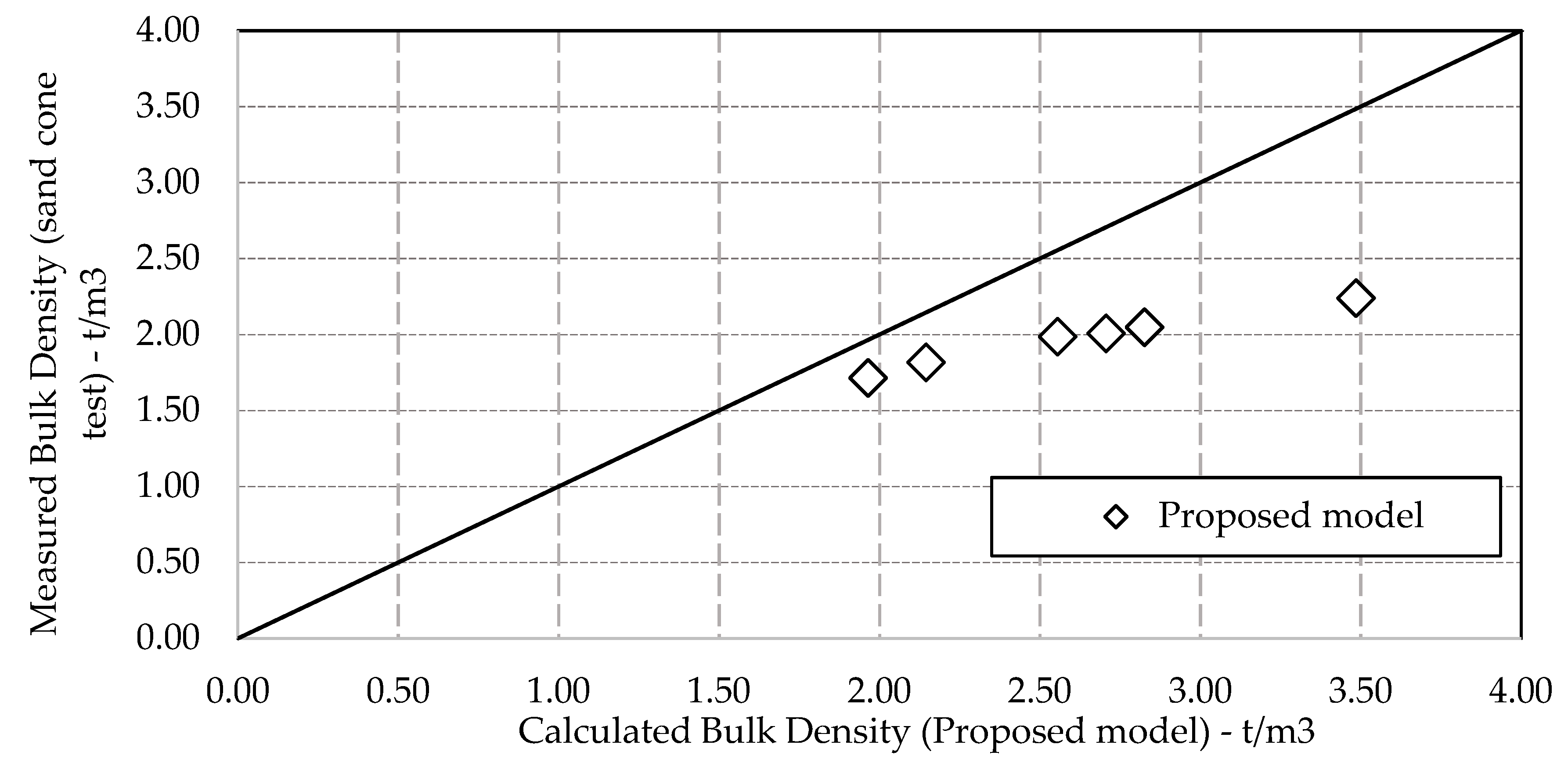
Compared to the lab-measured values mentioned in Table 2, higher bulk density was estimated from GPR data. Generally, the percent error ranged from 8 to 31% for the tested sections in the lab. A substantial error of 57% was observed for the specimen with the highest density. Figure 9 shows the comparison of measured and calculated bulk densities, along with line of equality.
Figure 9 shows that in spite of the proposed model gives higher results than the actual density, there’s a consistent relation that could be developed. Therefore, an exponential model was utilized to adjust the error between the calculated and measured bulk densities, as shown in Equation (12).
where, i and j = factors depend on soil type.
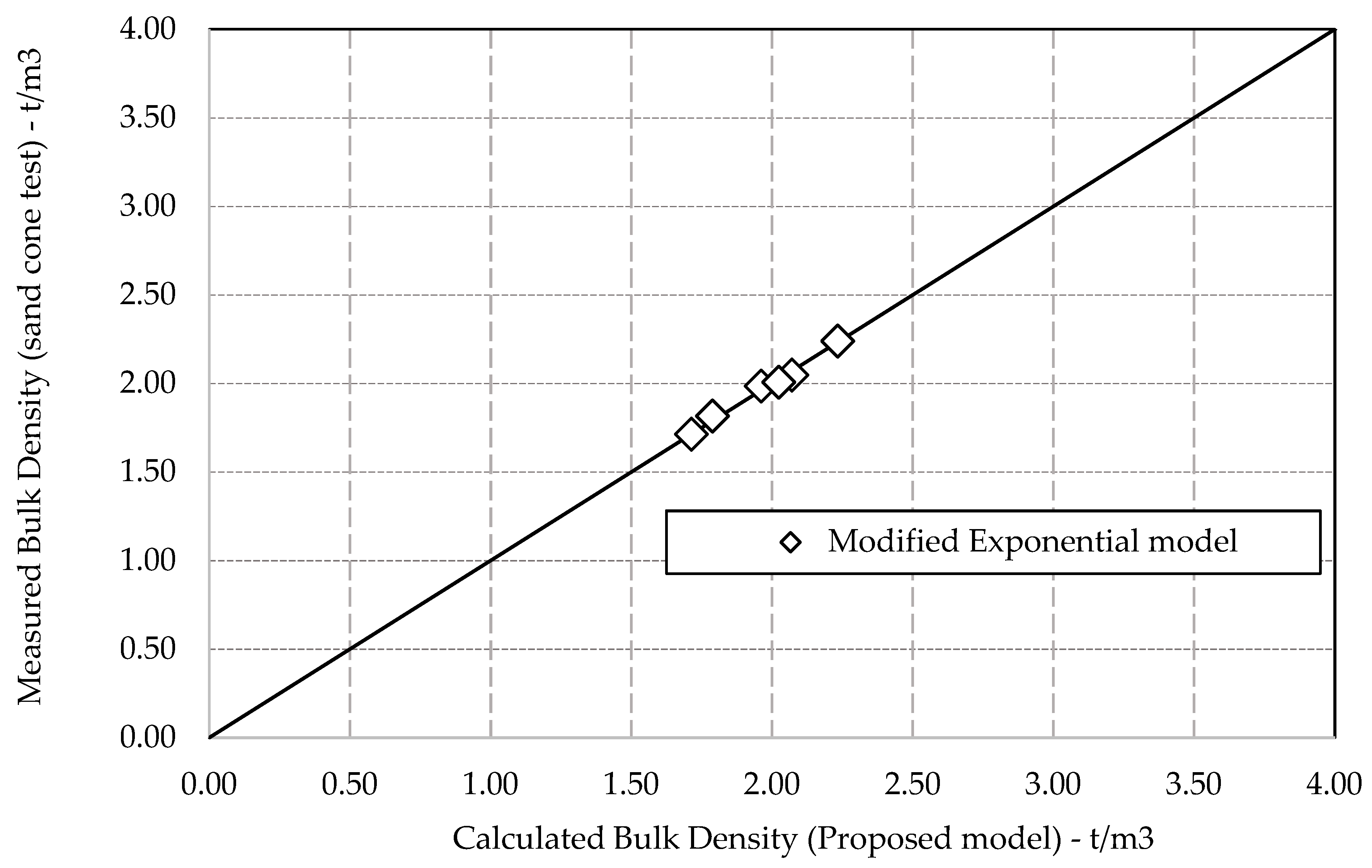
Based on the non-regression analysis, the fitting coefficients of i and j were estimated as 1.271 and 0.463, respectively, for the tested sample. The results of the exponential method are shown in Table 5.
The results from the modified exponential model (Equation (12)), show good agreement with those measured by sand cone lab test. As shown in Figure 10, this model gives a good estimate, with a maximum error of 2.1% of the measured bulk density.
7. Conclusions and Discussion
The GPR scanning technique has been used to assess the subgrade soils’ density. An air-coupled antenna operating at 2 GHz central frequencies has been utilized for investigation purposes. A numerical approach was tested to estimate the bulk density of subgrade soil. The soil densities estimated by GPR and measured by the sand cone method have less than 2.1% error for the MH soil tested.
According to the aforementioned results and conclusions, this technique has a high potential for several applications in civil geotechnical projects. To mention some of them, during construction of new roads it could be used for the quality control of subgrade layers compaction or for any compaction operations in several civil works. Also, it could be used in maintenance and rehabilitation decision making, by conducting periodical scan procedures in order to decide precisely when to perform rehabilitation.
Future research will examine the estimation of different soil types’ physical (density, water content) and mechanical (strength and elasticity) properties for more than soil type (laboratory and field), using different GPR antennas (air-coupled, ground-coupled) with different frequencies. The technique discussed in this paper constitutes a revolutionary technique with the potential for a new era in roads and geotechnical inspection methodologies.
Author Contributions
The authors confirm contribution to the paper as follows: Study conception and design, S.S.K.; data collection, A.A.; Analysis and interpretation of results, S.S.K. and A.A.; draft manuscript preparation, A.A. and S.S.K.; draft manuscript review and editing: A.A. and S.S.K.. All authors reviewed the results and approved the final version of the manuscript.
Funding
The work presented in this paper is part of a research project (RP 19-21) sponsored by the Georgia Department of Transportation. The contents of this paper reflect the views of the authors, who are solely responsible for the facts and accuracy of the data, opinions, and conclusions presented herein. The contents may not reflect the views of the funding agency or other individuals.
Acknowledgments
The authors would like to thank the many GDOT personnel that assisted with this study. A special thanks to Ms. Monica Flournoy, GDOT State Materials Engineer and Mr. Ian Rish, P.E., GDOT State Pavement Engineer.
Conflicts of Interest
The authors declare no conflict of interest. The funding sponsors had no role in the design of the study; in the collection, analyses, or interpretation of data; in the writing of the manuscript, and in the decision to publish the results.
References
- Abdelmawla, A.M.; Durham, S.A.; Kim, S. Estimation of Subgrade Soil Density Using Ground Penetrating Radar. In Proceedings of the 2019 ICSC Conference, Seoul, Korea, 17–19 July 2019. [Google Scholar]
- Benedetto, A.; Benedetto, F.; Tosti, F. GPR applications for geotechnical stability of transportation infrastructures. Nondestruct. Test. Eval. J. 2012, 27, 253–262. [Google Scholar] [CrossRef]
- AASHTO. Mechanistic-empirical pavement design guide: A manual of practice; American Association of State Highway Officials and Transportation Officials: Washington, DC, USA, 2008. [Google Scholar]
- Hu, J.; Vennapusa, P.K.; White, D.J.; Beresnev, I. Pavement thickness and stabilised foundation layer assessment using ground-coupled GPR. Nondestruct. Test. Eval. J. 2016, 31, 267–287. [Google Scholar] [CrossRef]
- Barman, M.; Nazari, M.; Imran, S.A.; Commuri, S.; Zaman, M.; Beainy, F.; Singh, D. Quality control of subgrade soil using intelligent compaction. Innov. Infrastruct. Solut. 2016, 1, 23. [Google Scholar] [CrossRef] [Green Version]
- Leng, Z.; Al-Qadi, I.L.; Baek, J.; Lahouar, S. Selection of Antenna Type and Frequency for Pavement Surveys Using Ground Penetrating Radar (GPR). Presented at the 88th Annual Meeting of the Transportation Research Board, Washington, DC, USA, 11–15 January 2009. [Google Scholar]
- Saarenketo, T. Using Ground-Penetrating Radar and Dielectric Prob Measurements in Pavement Density Quality Control. Transp. Res. Rec. 1997, 1575, 34–41. [Google Scholar] [CrossRef]
- ASTM D2487-17. Standard Practice for Classification of Soils for Engineering Purposes (Unified Soil Classification System); ASTM International: West Conshohocken, PA, USA, 2017; Available online: http://www.astm.org (accessed on 11 March 2019).
- Hogentogler, C.A.; Terzaghi, K. Interrelationship of load, road and subgrade. Public Roads 1929, 10, 37–64. [Google Scholar]
- EN ISO 14688-1:2002/A1:2013. Geotechnical Investigation and Testing—Identification and Classification of Soil—Part 1: Identification and Description—Amendment 1; Européen de Normalisation: Brussels, Belgium, 2013; pp. 3–4. Available online: http://78.100.132.106/External%20Documents/Intenational%20Specifications/British%20Standards/BS%20EN%20ISO/BS%20EN%20ISO%2014688-1-2002%20+%20A1-2013.pdf (accessed on 15 December 2019).
- EN ISO 14688-2:2004/A1:2013. Geotechnical Investigation and Testing—Identification and Classification of Soil—Part 2: Principles for a Classification—Amednment 1; Européen de Normalisation: Brussels, Belgium, 2004; pp. 8–10. Available online: http://78.100.132.106/External%20Documents/Intenational%20Specifications/British%20Standards/BS%20EN%20ISO/BS%20EN%20ISO%2014688-2-2004%20+%20A1-2013.pdf (accessed on 15 December 2019).
- Leng, Z.; Al-Qadi, I.L.; & Lahouar, S. Development and validation for in situ asphalt mixture density prediction models. NDT E Int. 2011, 44, 369–375. [Google Scholar] [CrossRef]
- EM GeoSci App Docs Page. Available online: https://em.geosci.xyz/content/physical_properties/dielectric_permittivity/dielectric_permittivity_factors.html, (accessed on 15 March 2019).
- Topp, G.; Davis, J.L.; Annan, A.P. Electromagnetic determination of soil water content: Measurements in coaxial transmission lines. Water Resour. Res. 1980, 16, 574–582. [Google Scholar] [CrossRef] [Green Version]
Figure 1.
Ground penetrating radar (GPR) Horn Antenna.

Figure 2.
SIR30 Road scan system.

Figure 3.
Subgrade soil preparation (a) soil placement, (b) soil compaction.

Figure 4.
Soil samples.

Figure 5.
Soil samples schematic diagram for reflections from layer interfaces in a typical pavement system [6].
Figure 5.
Soil samples schematic diagram for reflections from layer interfaces in a typical pavement system [6].

Figure 6.
Flow chart for the soil bulk density estimation process.

Figure 7.
Scanning and calibration for different samples.

Figure 8.
Amplitude for different soil samples.


Figure 9.
Measured vs. estimated (proposed) soil bulk density.

Figure 10.
Measured vs. Estimated (Exponential Model) soil bulk density.


Table 1.
Soil Index Properties.
| Specific Gravity | USCS Classification | Fines (%) | PL | LL | PI | Max Dry Density (kg/m3 (pcf)) | Optimum Moisture Content (%) |
|---|---|---|---|---|---|---|---|
| 2.76 | MH | 57.21 | 37.44 | 57.1 | 19.7 | 1853.3 (115.7) | 15.4 |
Table 2.
Sand cone test results.
| Sample | Bulk Density (γbulk) | Dry Density (γdry) | Compaction Obtained | Water Content | ||
|---|---|---|---|---|---|---|
| (t/m3) | (pcf) | (%) | (%) | |||
| BdS 1 | 2.240 | 139.8 | 1.871 | 116.8 | 100% | 20% |
| BdS 2 | 2.047 | 127.8 | 1.737 | 108.5 | 93% | 18% |
| BdS 3 | 1.985 | 123.9 | 1.673 | 104.4 | 89% | 19% |
| BdS 4 | 2.007 | 125.3 | 1.664 | 103.9 | 89% | 21% |
| BdS 5 | 1.817 | 113.4 | 1.564 | 97.6 | 84% | 16% |
| BdS 6 | 1.714 | 107.0 | 1.472 | 91.9 | 79% | 16% |
Note: BdS = Bulk density Sample
Table 3.
Dielectric constant results.
| Sample ID | Amplitude | Dielectric Constant (ε) |
|---|---|---|
| BdS 1 | 6,198,456 | 65.76 |
| BdS 2 | 5,896,713 | 45.77 |
| BdS 3 | 5,830,069 | 42.52 |
| BdS 4 | 5,739,976 | 38.60 |
| BdS 5 | 5,450,763 | 28.90 |
| BdS 6 | 5,298,273 | 25.08 |
Table 4.
Dielectric constant results.
| Sample ID | θ | w (Calculated) | Bulk Density (γbulk) Estimated | |
|---|---|---|---|---|
| t/m3 | pcf | |||
| BdS 1 | 71% | 20% | 3.48 | 217.6 |
| BdS 2 | 54% | 19% | 2.83 | 176.4 |
| BdS 3 | 52% | 19% | 2.71 | 168.9 |
| BdS 4 | 50% | 20% | 2.56 | 159.5 |
| BdS 5 | 44% | 20% | 2.14 | 133.9 |
| BdS 6 | 40% | 20% | 1.96 | 122.7 |
Note: εw = 80 (80–81), εs = 6 (5–8)
Table 5.
Exponential model results.
| Sample ID | i (γbulk Estimated)j | γbulk Measured. | Error % | ||
|---|---|---|---|---|---|
| t/m3 | pcf | t/m3 | pcf | ||
| BdS 1 | 2.29 | 142.8 | 2.24 | 139.8 | 2.10% |
| BdS 2 | 2.03 | 126.6 | 2.05 | 127.8 | 1.00% |
| BdS 3 | 1.99 | 124.3 | 2.01 | 125.3 | 0.80% |
| BdS 4 | 1.96 | 122.6 | 1.99 | 123.9 | 1.10% |
| BdS 5 | 1.86 | 115.8 | 1.82 | 113.4 | 2.00% |
| BdS 6 | 1.72 | 107.5 | 1.71 | 107.0 | 0.50% |
© 2020 by the authors. Licensee MDPI, Basel, Switzerland. This article is an open access article distributed under the terms and conditions of the Creative Commons Attribution (CC BY) license (http://creativecommons.org/licenses/by/4.0/).
Share and Cite
MDPI and ACS Style
Abdelmawla, A.; Kim, S.S. Application of Ground Penetrating Radar to Estimate Subgrade Soil Density. Infrastructures 2020, 5, 12. https://0-doi-org.brum.beds.ac.uk/10.3390/infrastructures5020012
AMA Style
Abdelmawla A, Kim SS. Application of Ground Penetrating Radar to Estimate Subgrade Soil Density. Infrastructures. 2020; 5(2):12. https://0-doi-org.brum.beds.ac.uk/10.3390/infrastructures5020012
Chicago/Turabian StyleAbdelmawla, Ahmad, and S. Sonny Kim. 2020. "Application of Ground Penetrating Radar to Estimate Subgrade Soil Density" Infrastructures 5, no. 2: 12. https://0-doi-org.brum.beds.ac.uk/10.3390/infrastructures5020012