1. Introduction
In recent years, there has been a strong interest in long term monitoring of in-service pavements, and in using non-destructive tools to evaluate pavement performance. Several non-destructive testing methods have been developed to measure the surface deflection and to assess the structural capacity of asphalt pavements. The most commonly used are static measurement methods like the Benkelman beam and impulse loading methods like the FWD. These methods present the advantage of reproducing closely the loading conditions and the stress state in the pavement. However, these techniques can only measure the deflection at discrete locations, and require interrupting the traffic. Hence, these techniques are costly and the measurements are recorded infrequently, i.e., only once per year or two years.
The need to collect the data without disruption of the traffic flow and to measure the response continuously, under normal traffic, has led to the development of pavement instrumentation with different sensors. Strain sensors and temperature probes are the most commonly used devices to instrument and characterize pavement conditions. Some applications have also used piezoelectric sensors to measure stresses and strains in pavement layers, to monitor the fatigue damage of pavements [
1,
2,
3].
In paper [
4] the work focuses on the vibro-acoustic response of transportation infrastructure. It uses a lightweight deflectometer to identify the localization of cracks and variations in the elastic modulus of the pavement by using the road traffic noise as its vibration source and by the help of microphones drilled in the upper layer of the pavement which record the vibration noise. These vibrations are analyzed to identify the severity of the cracks and the level of damage. In [
5], the author discusses an approach using the falling weight deflectometer to back-calculate the layer moduli using a probabilistic approach. The static and dynamic deflection bowls are used from the FWD data sets, for the back-calculation of layer moduli and a comparative study is made to accurately back-calculate pavement layer moduli.
The work of [
6] focuses on using a laser dynamic deflectometer that has four laser Doppler sensors and a rigid beam to measure the deflection velocity and then compute the deflection basin. It defines the relation between the measured values and the position of the sensors and analyzes the effectiveness of both dynamic and static calibration methods on measurement accuracy. It also studies the impact of the traffic speed on obtained results and concludes that both methods produce effective results.
Geophones and accelerometers are designed to measure the inertial vibrations of the pavement and used in research studies to calculate the deflection basin of the pavement caused by the passage of wheel loading. In the work done by Lie et al. [
7], an experimental setup with an array of geophones was used to measure the vibrations during the passage of a known vehicle load. The responses, along with a mobile load simulator and a back-calculation tool, were used to measure the pavement deteriorations.
The work done by Arraigada et al. [
8] consisted in measuring the pavement deflections using accelerometers and deflectometers. They also used a visco-elastic pavement model to fit the measurements obtained with the deflectograph. This research points out the difficulties in converting the acceleration into deflections, due to the integration process and noise and drift in the signal. A spline-based correction method was used to convert the acceleration signal into deflections.
The work done by Levenberg [
9] describes the use of an accelerometer embedded in asphalt pavement. The loading is applied by a vehicle of known dimensions and weight passing near the accelerometer. These accelerations could then be used for back-calculating the pavement layer properties, without converting the measurements into deflections, which eliminates the integration and amplification errors.
Ngoc Son et al. [
10] use geophones to measure pavement deflections and to monitor evolution of pavement layer properties with respect to traffic and environmental conditions. They also focus on the need to improve signal processing to get accurate results using geophones.
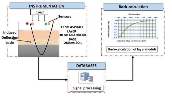
This work is part of a research that aims at developing a monitoring system for asphalt pavements focusing on the use of geophones and accelerometers for measuring deflections and accurately back-calculating pavement layer moduli. The sensors are evaluated first in the laboratory, and then on an accelerated pavement testing facility, under various testing conditions. In each case, a reference sensor is used to evaluate measurement accuracy. In the laboratory tests, a laser displacement sensor is used and for the full-scale accelerated pavement tests, an anchored deflectometer is installed. These reference sensors have a good accuracy, but their deployment on a real road site is difficult.
The main advantage of using accelerometers or geophones is the ease of embedment on a real pavement before and even after the construction of the pavement, with a possibility of having continuous pavement monitoring, under real traffic. The determination of the type of vehicles and their corresponding speeds is also possible with the aid of these sensors.
Objectives
As in-service roads advance with time, their initial mechanical properties (modulus, fatigue resistance, etc.) are highly affected. Traffic loads, environmental effects, such as temperature and moisture variations, and aging cause structural damage and surface wear. For this reason, it is important to measure the pavement response like deflection to predict pavement performance and continuously monitor the health of the pavement for condition-based maintenance decisions. Presently, deflections are mainly measured by the FWD and deflectograph, and the results are used for back-calculation of pavement layer properties. The drawback of these methods is that the measurements require to close the road to traffic, and that the road cannot be monitored continuously, measurements being made at best once a year. Using total deflection data obtained from accelerometers or geophones, as demonstrated in this paper, could facilitate the measurement of pavement response, and enable continuous monitoring of pavement condition.
To test the possibility to monitor pavement layer properties, deflection basins obtained from the geophone and accelerometer measurements, are used to back-calculate pavement layer moduli. For that purpose in this work,
Section 2 presents the selection of suitable sensors for measuring the vertical displacement.
Section 3 presents pavement response calculations, which are used to determine the theoretical deflection response of bituminous pavement, under heavy vehicle loading.
Section 4 describes the laboratory tests done with the selected sensors and the experimental protocol. The sensor measurements are converted accurately to deflections using signal processing techniques, as described in
Section 5. The sensors are also tested at the accelerated pavement facility as explained in
Section 6 and using these responses, the pavement design software Alize is used for the back-calculation of pavement layer moduli, described in
Section 7.
2. Geophones and Accelerometers Selected for Pavement Deflection Measurement
Selecting the Sensors to Measure Pavement Deflection
There are several criteria to consider in order to select the appropriate geophones and accelerometers for the application of deflection measurement:
The typical deflection levels are between 0.1 and 1 mm, hence sensors should be sensitive enough to carry measurements in this range.
The resonance frequency of the sensors should be low when compared to the frequency of the deflection signals (typically between 2 and 20 Hz).
The sensors should have a small size, to facilitate embedment in the pavement layers
Durability, mechanical resistance, and stability of the sensor response are also important factors, as pavement measurements need to be performed over periods of several years.
Relatively limited cost, to enable widespread use of this type of instrumentation.
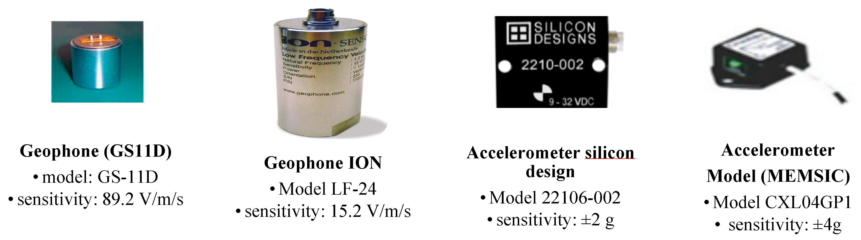
These criteria have led to select two types of geophones and two accelerometers, described in
Figure 1.
3. Pavement Modelling with Alize
There is a number of technical standards and documents followed for pavement structural design in France. In order to evaluate the response of the sensors mentioned and to define a reference deflection signal for conducting laboratory tests, the linear elastic software Alize is used [
11]. This software is based on the theory of Burmister, which defines the solution for axisymmetric problems for a single uniform circular load pressure [
12]. For this reason, a multilayer, linear elastic, semi-infinite and continuous pavement model is modeled using Alize. The interfaces can be considered bonded or sliding, depending on the pavement material being used. For this work, we have used bonded interfaces. It also uses a static pressure load on the pavement model to calculate the mechanical responses like horizontal and longitudinal strains and deflections. This software also includes a procedure for the back-calculation of pavement layer moduli.
The typical flexible pavement structure used to calculate the pavement response is defined in
Table 1. The layer moduli correspond to standard values used in the French pavement design method for a wearing course bituminous concrete (BBSG), an unbound granular material of category 2, and a subgrade of intermediate bearing capacity [
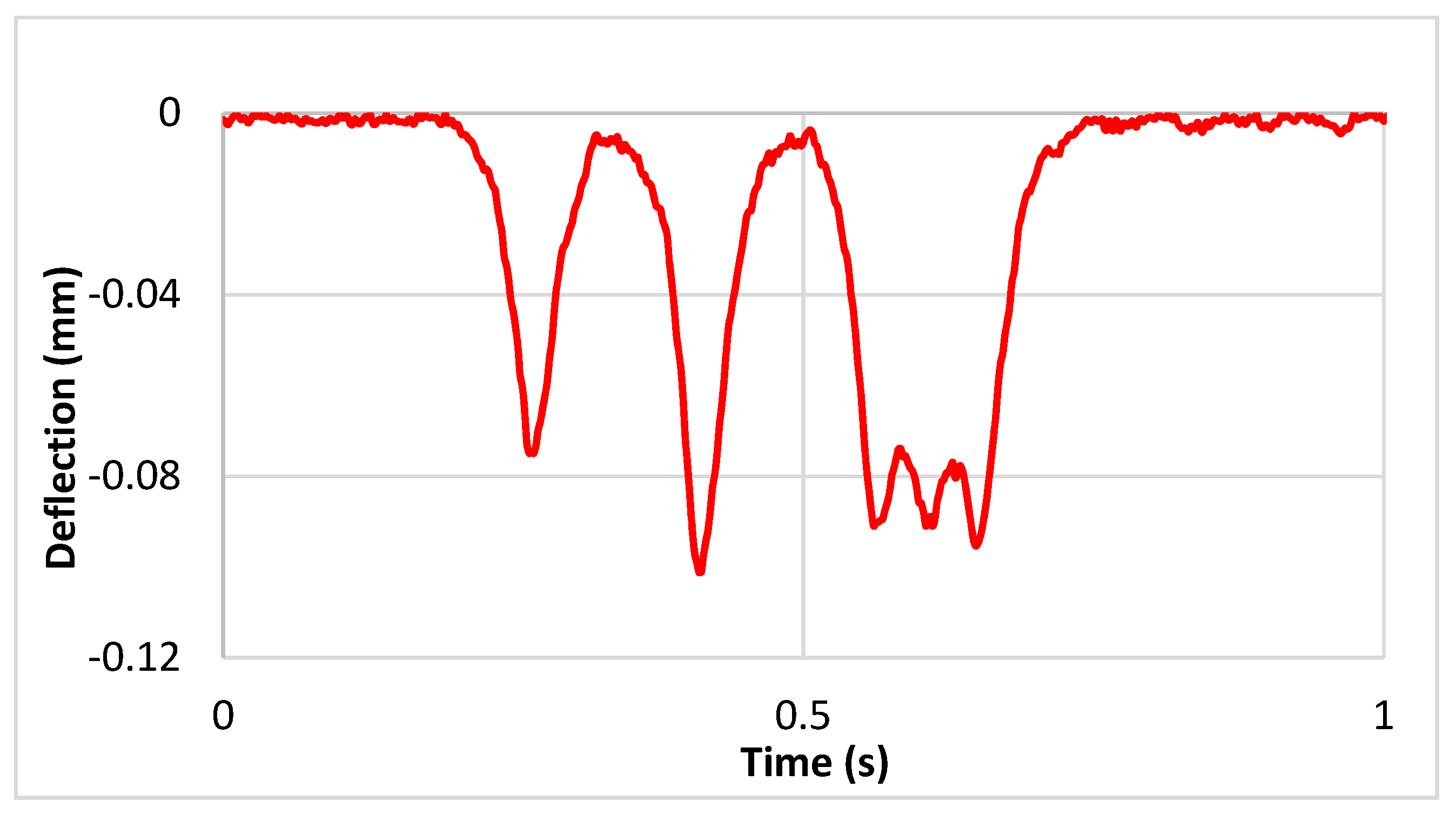
13]. The Poisson ratio was taken equal to 0.35 for all the pavement layers. The vehicle load considered is a 5-axle semi-trailer vehicle, with a total load of 40 tons. The deflection obtained with these parameters is defined in
Figure 2.
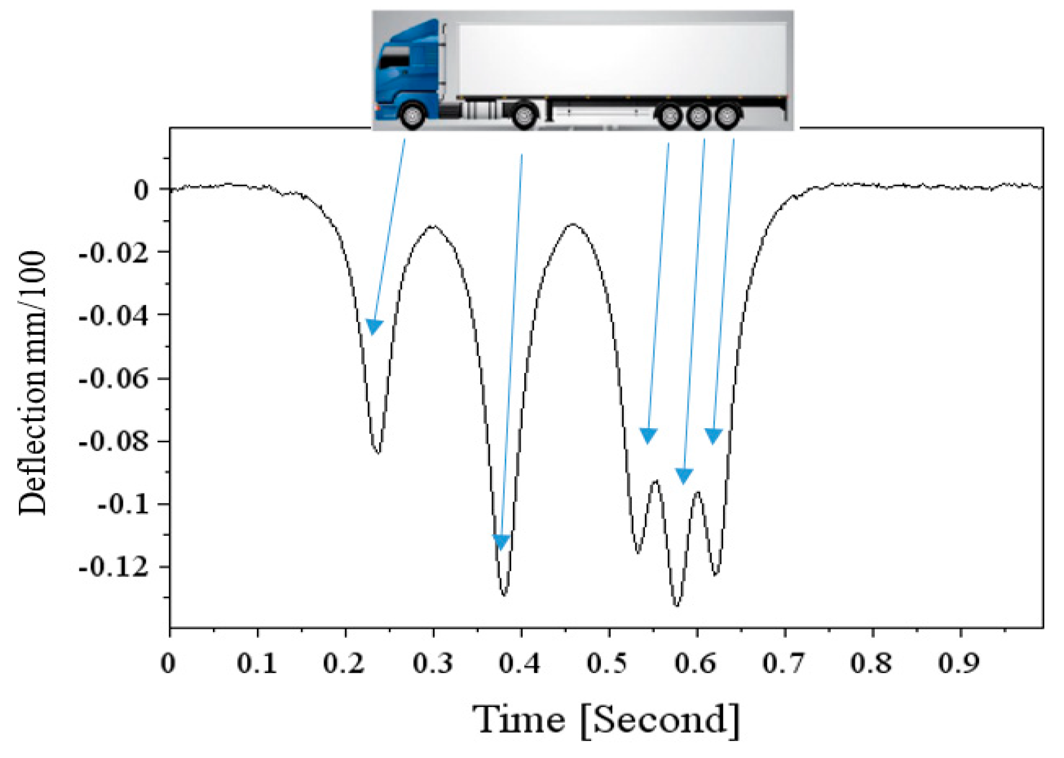
Displacement Signals
Figure 2 presents a typical deflection basin of the pavement, during the passage of a 5-axle heavy vehicle, generated with the ALIZE Software. The signal presents five peaks in the downward direction, corresponding to the five axles of the vehicle. The amplitude of the deflection depends on the axle loads, and the vehicle speed. For the geophones and accelerometers, the objective is to integrate the signals, in order to convert them into correct deflection values. As each negative peak in the signal corresponds to one axle of the vehicle, vehicle silhouettes can also be identified by counting and matching these peaks.
4. Laboratory Tests
The mechanical sensors come out with a predefined set of characteristics given by the manufacturers. However, it was considered important to verify the properties of the sensors, for typical pavement loading conditions, before installing them on an actual test site. In the application for pavement instrumentation, the sensitivity of the sensors is of utmost importance, due to the low displacement and acceleration levels. In addition, the signal to noise ratio of the sensors, with the actual acquisition system, and in real measurement conditions, needed to be determined. These tests were performed with different signal amplitudes and frequencies corresponding to typical heavy vehicle loading.
The tests were carried out at IFSTTAR using a vibrating table, with a hydraulic actuator, which applies the displacement to the horizontal plate with sensors installed on it. The responses of the different sensors were compared with the measurements of a reference Keyence laser displacement sensor. The following characteristics were determined:
The sensitivities of the geophones and accelerometers.
Signal responses for different amplitudes and velocities.
The intrinsic parameters like low-frequency noise that affect the response of the devices.
The tests on the vibrating table were carried out using controlled displacement signals, reproducing the deflection created by a 5-axle semi-trailer truck. These deflection signals were defined using pavement calculations, performed with the Alize pavement design software for the pavement structure in
Table 1. A signal of realistic shape was thus produced, and then applied at different amplitudes and frequencies, to simulate different vehicle loads and speeds.
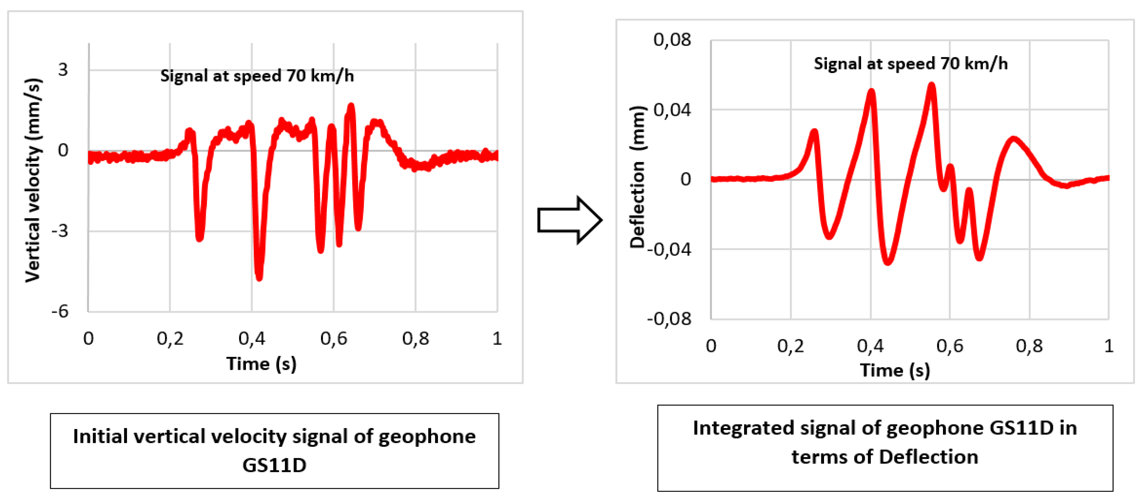
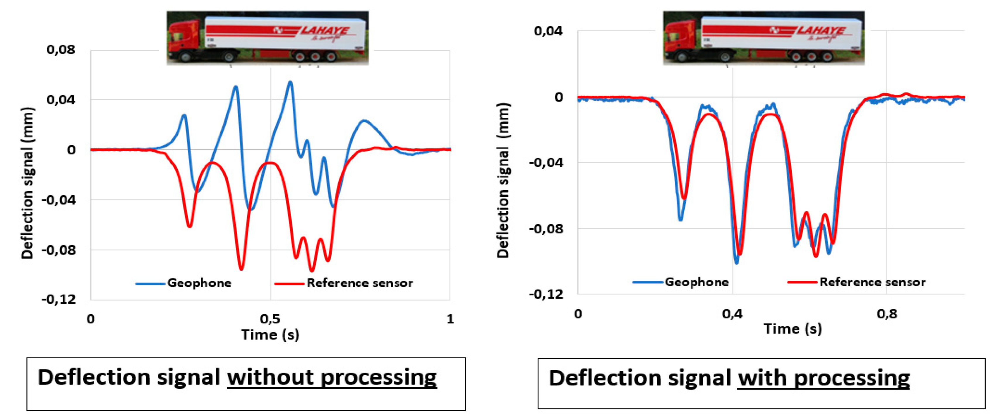
Four sensors can be tested at the same time on the vibrating table, as the acquisition system has four channels. Out of four, one channel was reserved to the Keyence laser sensor, used as reference to measure the displacements of the vibrating table. The measurements of the geophones and accelerometers require some treatment in order to convert them into appropriate values of vertical displacements or deflections. The measurements are to be integrated from velocity and accelerations into vertical displacements (deflections). For analyses purpose,
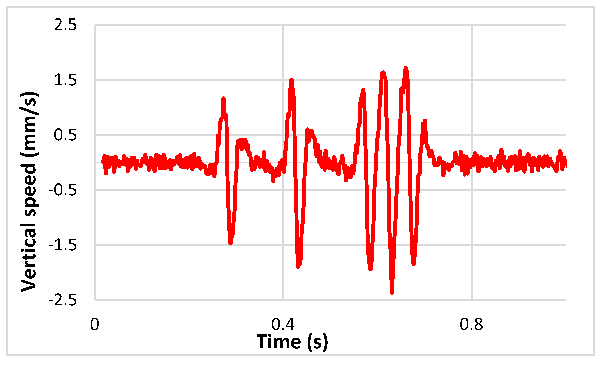
Figure 3 represents a raw geophone signal (measured displacement velocity), and the signal obtained after a simple integration. The same trend is observed for the values of acceleration after integration. It can be seen that after a simple integration process, the displacement signal obtained does not correspond exactly to the reference signal applied to the vibrating table (signal calculated with Alize). As can be seen in
Figure 3, the amplitudes of the peaks differ from the reference signal, and the shape of the signal is also different, showing some positive (upward) displacements. These upward movements are not realistic as only a downward displacement is applied to the sensors. The differences between the reference signal and the sensor signal are due to two main reasons:
- (1)
The direct integration process tends to attenuate the low-frequency components of the signal [
8]. The integration process also introduces a constant, and thus adds a continuous component to the signal. This may explain the unrealistic shape of the signal, with positive displacement values.
- (2)
In addition, as can be seen, the raw geophone and acceleration signals present some noise, which can also lead to inaccurate results. The noise generates high-frequency variations in the response signals, which do not represent the actual vertical displacement of the pavement and needs to be filtered [
14].
5. Signal Processing and Filtering of Sensor Responses
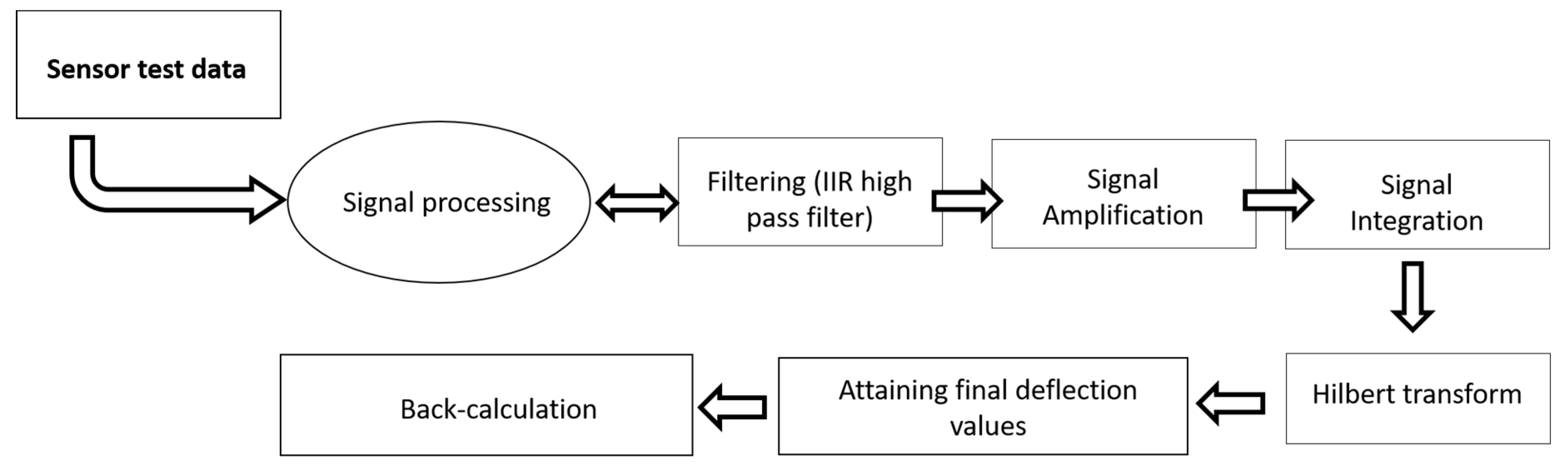
5.1. Scheme to Convert the Sensor Response into Vertical Displacement and Improving the Accuracy
One of the objectives of this work is to find an appropriate method to convert the vertical velocities and accelerations into realistic values of vertical pavement deflections, which can then be used for back-calculation of the pavement layer moduli, as described in
Figure 4. For that, a signal-processing method has been tested and a methodology to correct the measurements has been developed. This procedure has been applied to the measurements of the two types of geophones used (Geospace GS11D and Ion LF-24) and two types of accelerometers (MEMSIC and CXL04GP1). In the following figures, explaining the treatment procedure, only the responses obtained with the geophone GS11D are shown for illustration. This methodology is described in the following steps.
Step1: Filtering of the Signals
The first step consists in suppressing the lower frequency components of the signal using a recursive filter. The advantages of using Infinite Impulse Response (IIR) filter are that the noise suppression of the filtering is very low and the computation is faster [
15]. One of the downsides of using the IIR filter could be having unequal phase delays at each frequency component. For this reason, a zero-phase shifting filter is used, which uses forward and reverse filtering processes to compensate for the delay. As the output is created with a significant delay, it is fed back to the filter, to reverse the data points in time and align the signal to its original phase. The first pass performs the forward direction filtering using IIR filters and bypassing this signal through a zero-phase shift filter the backward filtering is achieved. In this work, an IIR highpass Chebyshev filter gave the best results, as it allows certain frequencies to pass and suppresses the lower frequencies containing noise and unwanted frequency content. It was observed that the cut-off frequency of the filter has a huge impact on the filtering process, and needs to be adapted to the vehicle speed. For low speeds, a cut-off frequency of 4.5 Hz is selected, which is increased as the speed is increased. For the maximum speed (20 m/s), a cut-off frequency of 20 Hz is used. The
Figure 5 shows the signal after filtering.
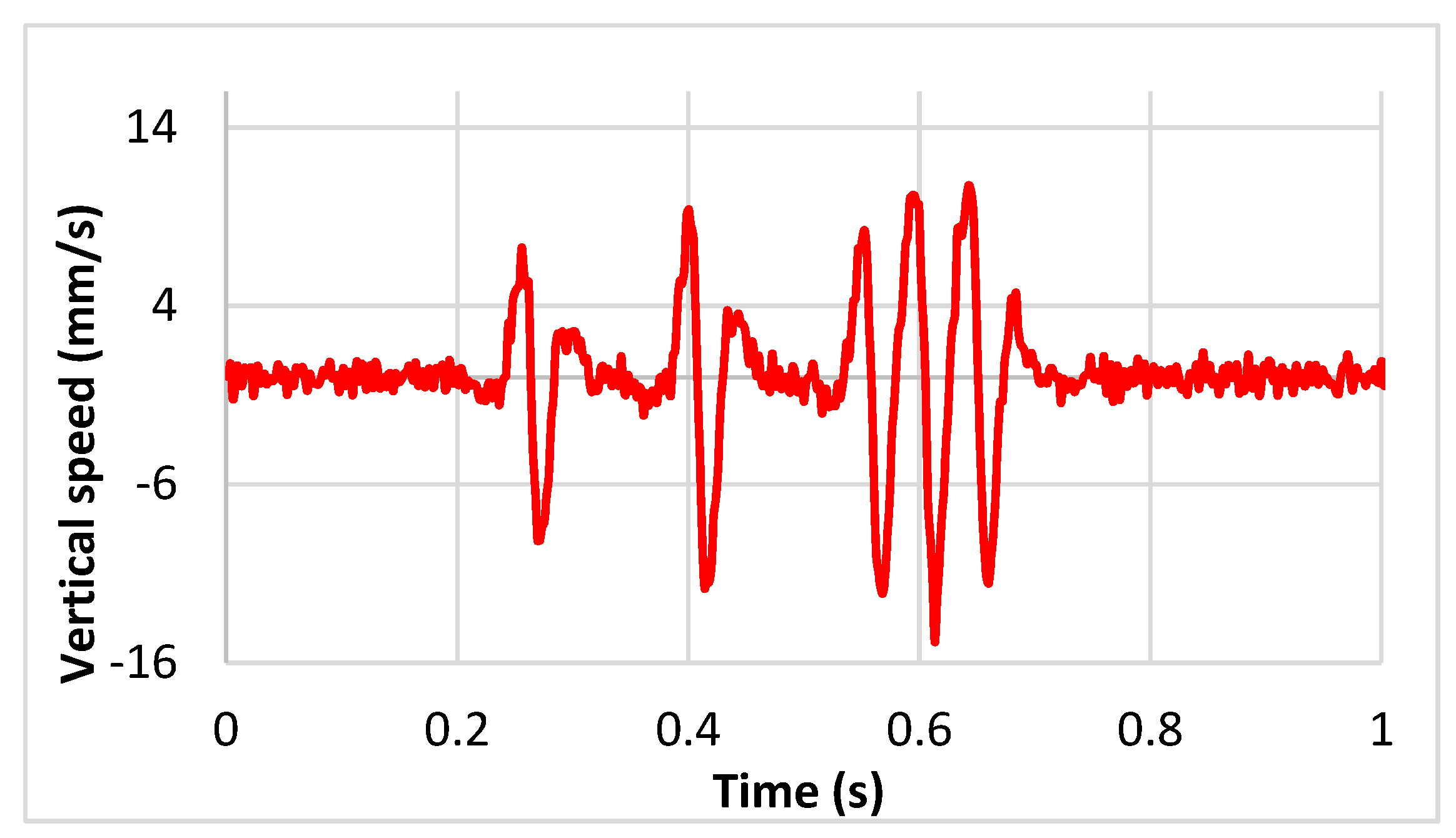
Step 2: Signal Amplification
It was observed that when the cut off frequencies are kept lower than the values indicated above, the noise was not sufficiently reduced. Hence, the shape of the signal was deteriorated. With high cut off frequencies, filtering improved the overall shape of the signal but reduced the amplitude of the signal. When the final filtered signal was compared to the reference signal, the amplitude was lower. For this reason, after filtering, the signal had to be amplified (by a linear constant amplification factor), to keep the initial amplitude as shown in
Figure 6.
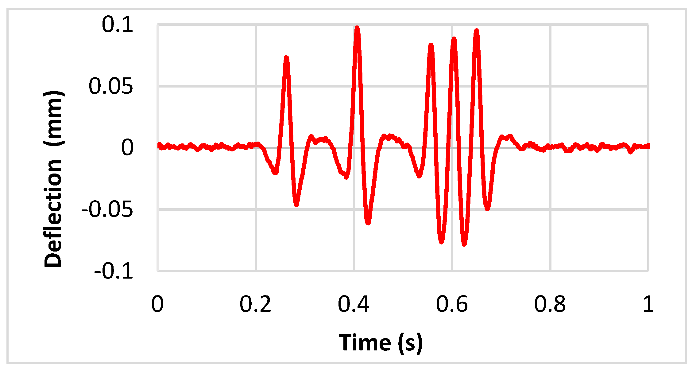
Step 3: Signal Integration and Detrending
After filtering, the vertical velocity is integrated to be converted into vertical displacement and the vertical acceleration is double integrated in a similar manner, to get the displacement. Simply integrating and double integrating the velocity and acceleration would increase small frequencies in the signal as well. Hence pre-processing is necessary before the integration of the signals.
As mentioned above, the integration step adds a continuous component to the signal as described by Equations (1) and (2). Hence, a detrending function is applied to suppress this continuous component. The signal after integration and detrending is shown in
Figure 7.
where V is the velocity, A is the acceleration, d is the displacement and ∆t is the difference in time.
Step 4: Application of the Hilbert Transform to the Signal
Due to the oscillations observed in the signals of the geophones and accelerometers, it seemed appropriate to use the Hilbert transform, to eliminate these oscillations from the sensor response. Time and frequency data analysis using the Hilbert transform specifically for structural health monitoring application has shown favorable results for interpreting structure response [
16]. Other applications of the Hilbert transform for vibration analysis include machine diagnosis, signal decomposition and industrial applications like health monitoring of powering systems [
17]. The common application of the Hilbert transform is the demodulation operation for extracting the envelope of the initial signal. As the oscillations detected in the signal from the sensors recall those of modulated signals, hence the Hilbert transform is used in our study. This function shifts the phase component of the signal by ±90 degrees, and thus the Hilbert transform of a sine signal would be a cosine signal with the same magnitude. Hence, when the signal is combined with its Hilbert transform the periodical oscillations in the signal are removed and the upward lifts in the signal are eliminated. In the time domain, the signal is the convolution of the signal and the Hilbert transform of the signal as expressed in Equation (3), where X(t) is the Hilbert transform H of the signal x(t)
where h(t) =
.
In the frequency domain, it is obtained with the Fourier transform and corresponds to the multiplication of the complex signal by –jsgn(w), where the signum function (sgn) is defined by Equation (4) [
18]. This multiplication produces a phase shift of the signal by ±90° or
, to generate the Hilbert transform. Hence, in the frequency domain, the Hilbert transform is actually a phase shift of the real signal.
The principle of the Hilbert transform is to combine a signal that is the real part (analytical signal) of the signal and an imaginary part of the signal used to extract the envelope of the signal. Hence, the corrected signal is given by:
The corrected signal at the end of the process S
a (t) corresponds to the envelope of the signal s(t),. This analytical signal is determined by the amplitude (A) and phase Ø, defined by
And the phase is given as
This function A also describes the dynamical behavior of amplitude modulation of the signal. This is why it is also known as the amplitude of the envelope. The function of phase is a measure of the signal at an instant in time and is therefore known as the instantaneous phase [
19]. In this case, this treatment drastically improves the shape of the signal, and leads to a response close to the theoretical deflection under a five-axle vehicle, as evident in
Figure 8.
5.2. Comparison of the Reference Laser Sensor with the Improved Measurements
Finally, the proposed correction procedure has been applied to the geophone and accelerometer signals obtained at different speeds and amplitudes, and the results have been compared with the reference deflection values obtained with the Keyence Laser sensor (
Figure 9). Generally, the procedure improves the geophone and accelerometer measurements significantly and leads to realistic signal shapes and displacement amplitudes, as described in the section below.
5.3. Results
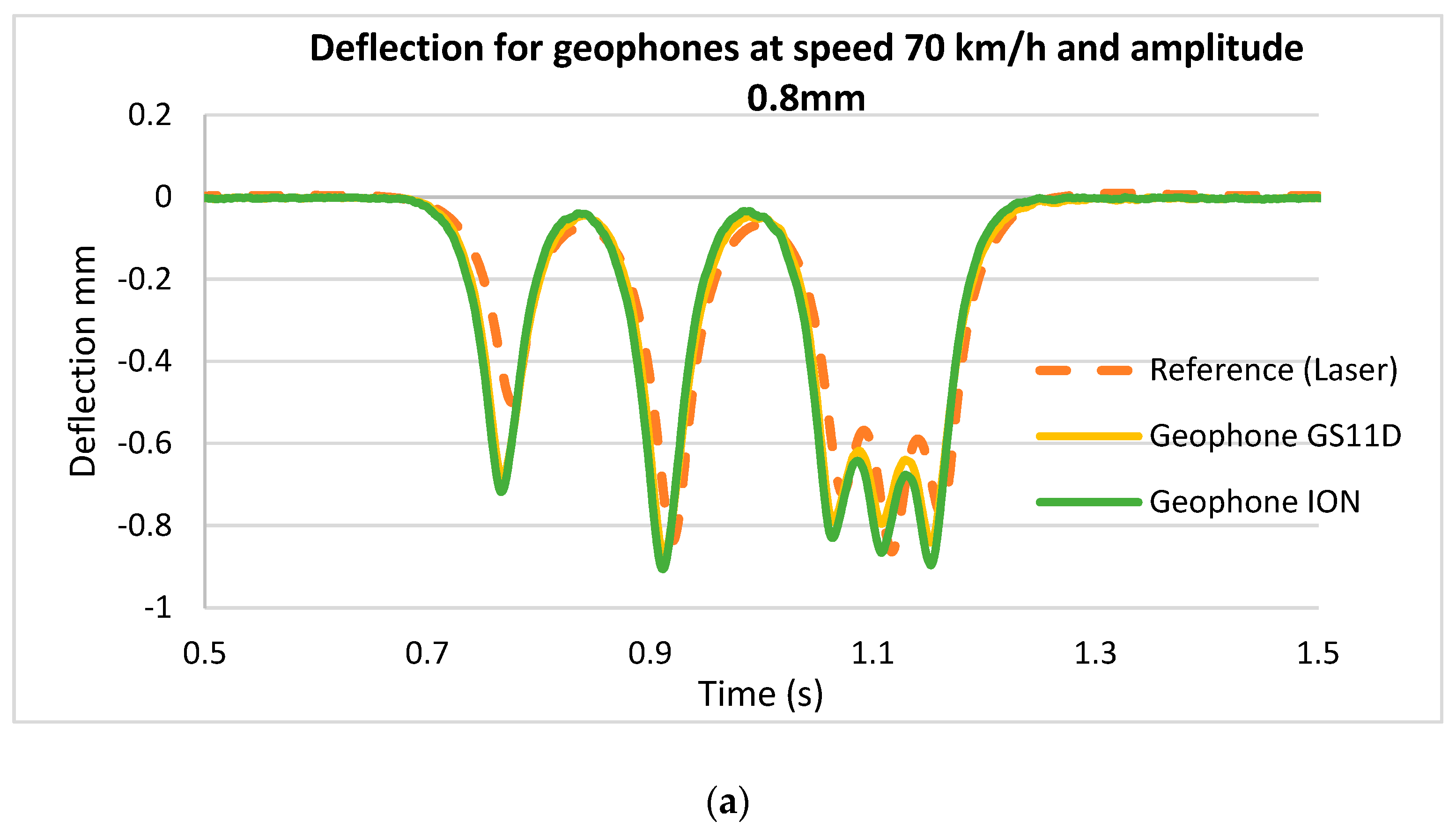
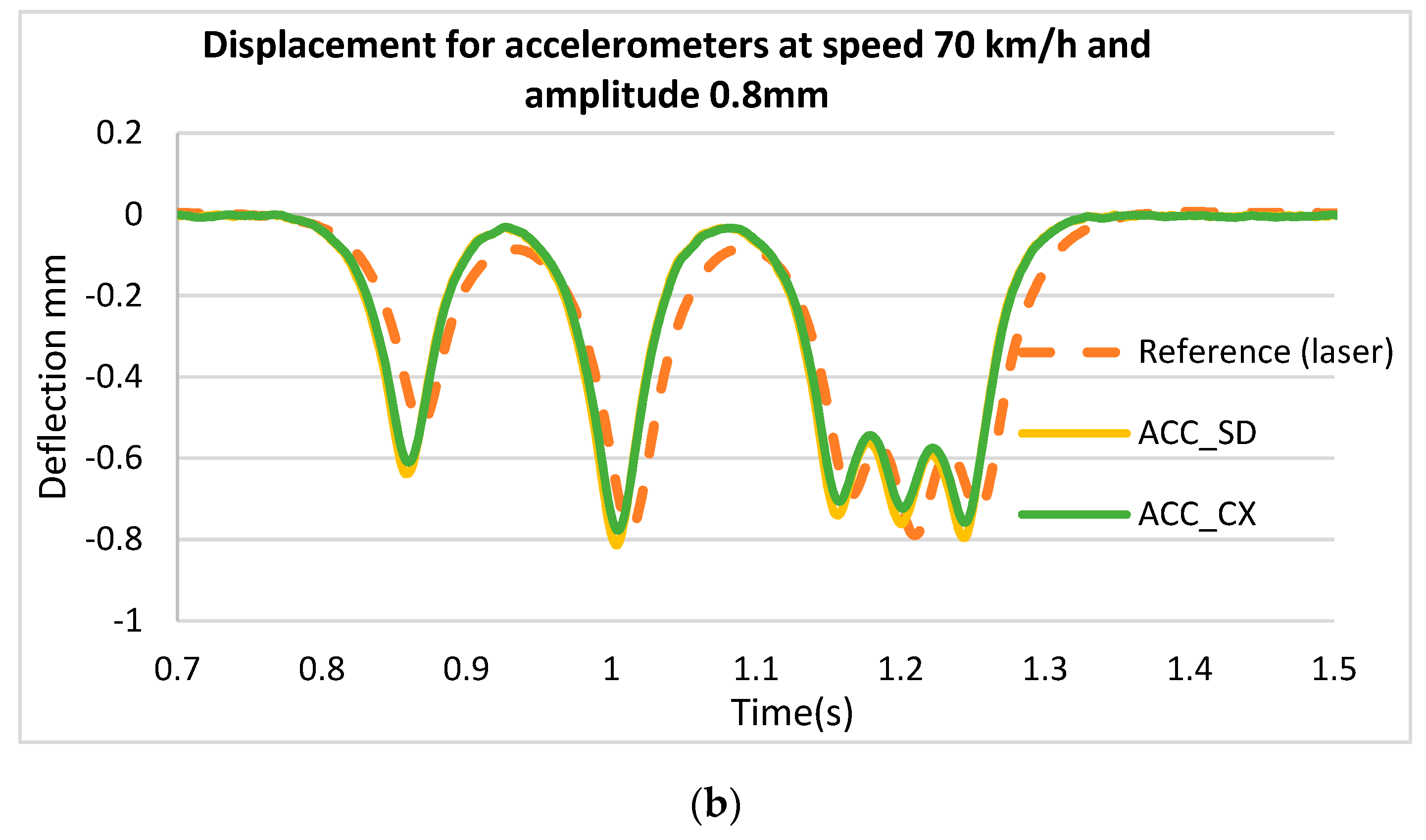
This section presents examples of laboratory results, namely displacement values obtained for a speed of 70 km/h (approx. 20 m/s), for the two geophones and two accelerometers (see
Figure 10). These values are treated in the same manner as described in
Section 5.1. The treated signals are compared with the response of the Keyence laser displacement sensor and it is important to note that the treatment procedure is the same for all the amplitudes and speeds. The parameter which is different is the cut-off frequency of the filter, which needs to be increased as the speed increases. With different cut off frequencies, the amplification factors are varied and the optimal shapes of the signals are obtained, which are very close to the reference signals.
6. Accelerated Pavement Tests
6.1. Experimental Setup
The sensors described in
Section 2 (two geophones and two accelerometers) were embedded in a pavement structure tested on the IFSTTAR accelerated pavement testing (APT) facility. A reference, anchored deflectometer was also installed, to serve as a reference for the measurement of the deflection response.
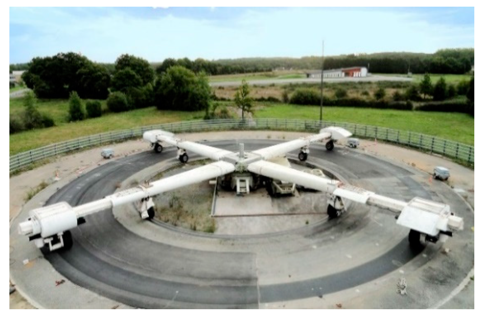
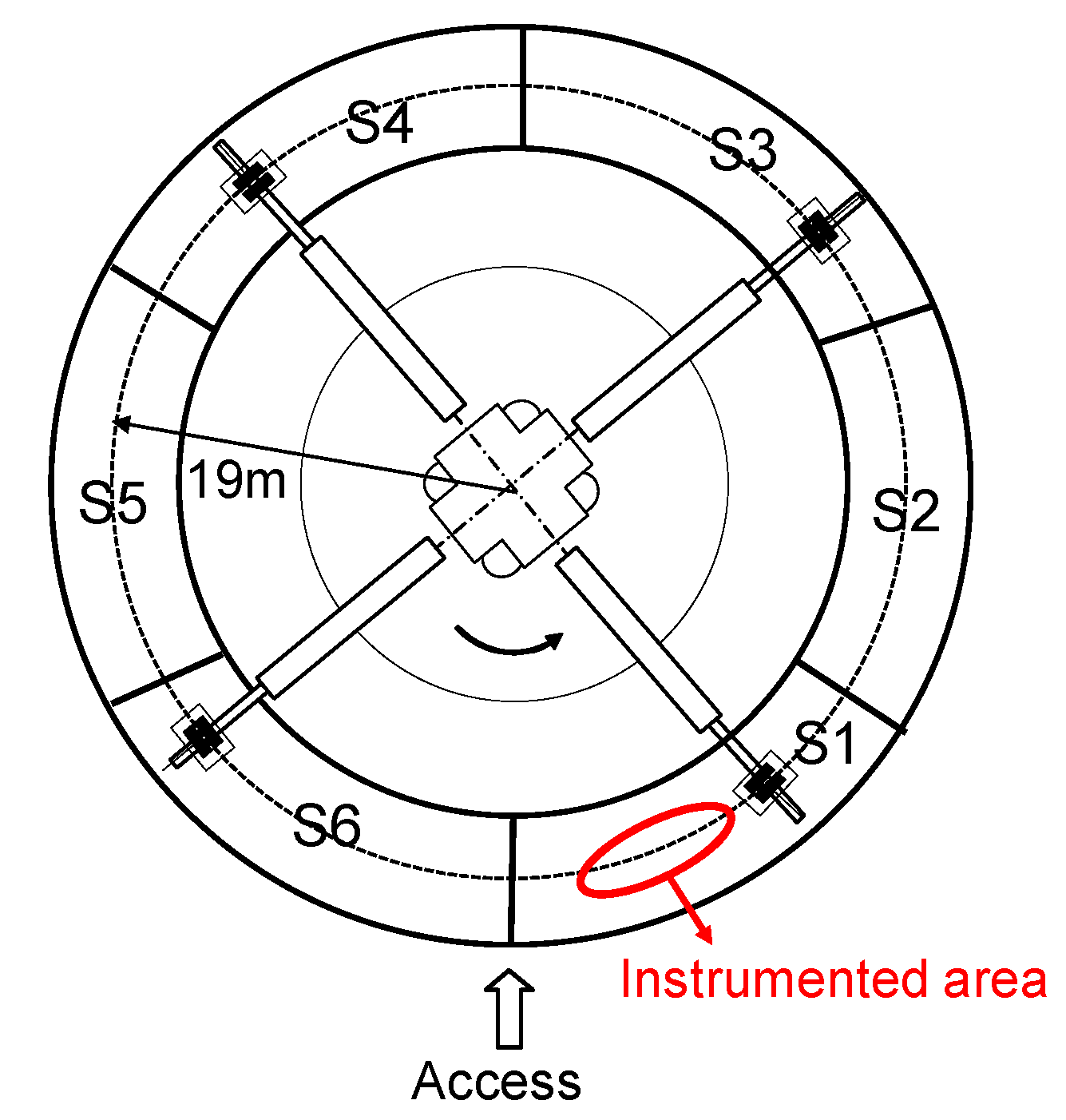
The IFSTTAR APT, or fatigue carrousel, is a circular outdoor testing facility that consists of a circular test track of 40 m diameter and a central loading system (
Figure 11). The carousel has four identical loading arms, each equipped with a wheel carriage which can carry loads up to 13 tons.
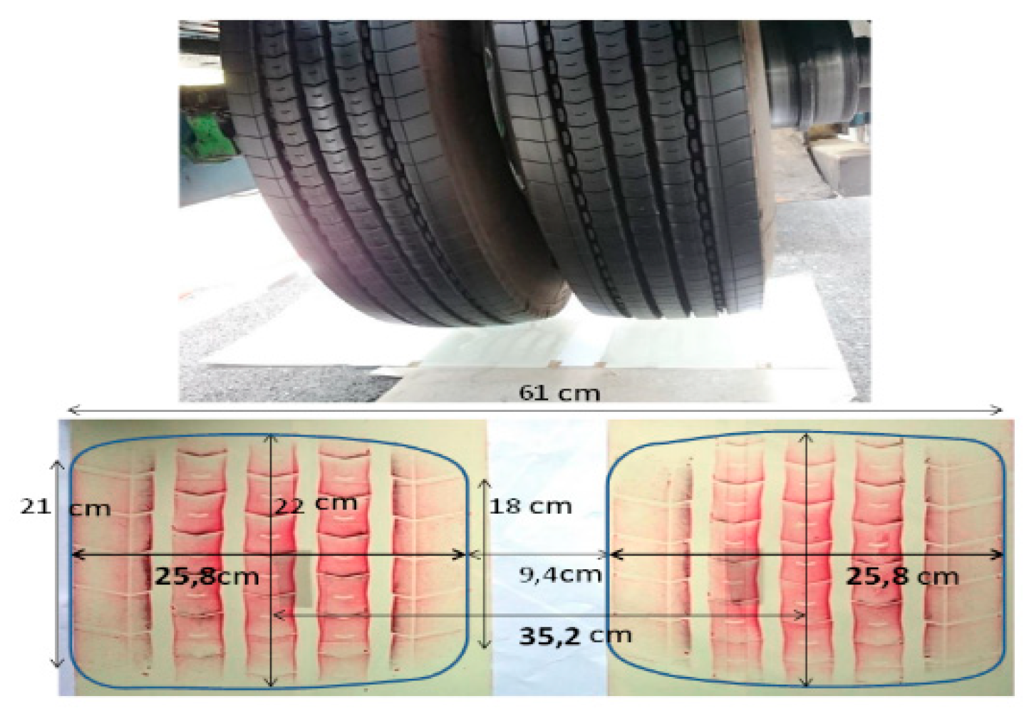
The wheel carriages can comprise different wheel arrangements. In this experiment, dual wheels were used. The wheel dimensions are shown in
Figure 12, and the tire-pavement contact stress was equal to 0.6 MPa. The sensors were installed in one of the six test sections of the carousel, called Section S1 (
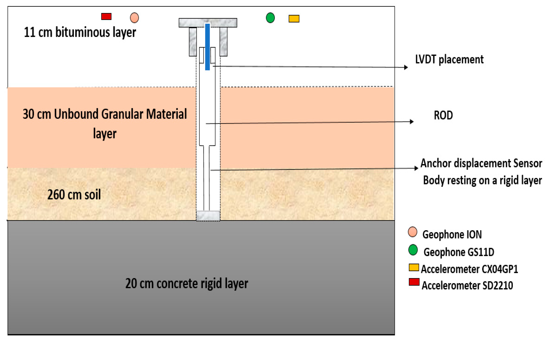
Figure 13). This pavement section was 22 m long and consisted of an 11 cm thick asphalt concrete layer, and a granular base. The positions of the geophones, accelerometers and anchored deflectometer on the pavement section are shown in
Figure 14. The geophones and accelerometers were placed 1 cm below the pavement surface, in the center of the wheel path. Each sensor placed in small boreholes drilled in the asphalt layer, and sealed with resin. A small trench was also cut in the pavement, up to the pavement edge, and the sensor cable was inserted in this trench and sealed with resin. The anchored deflectometer consists of an LVDT which is connected to a rod, anchored at a significant depth (here three meters), and which measures the total vertical displacement between the pavement surface and the bottom of the rod, supposed fixed.
The characteristics of the pavement structure where the sensors were installed are given in
Table 2. The characteristics of the pavement layers were determined using the following tests:
Thicknesses of the different layers were determined from the controls made during and after construction
Bituminous material complex moduli were determined from laboratory tests on the field produced mix
The moduli of the granular layer were determined by back-calculation, from FWD measurements
The moduli of the subgrade were determined from Benkelman beam deflection measurements.
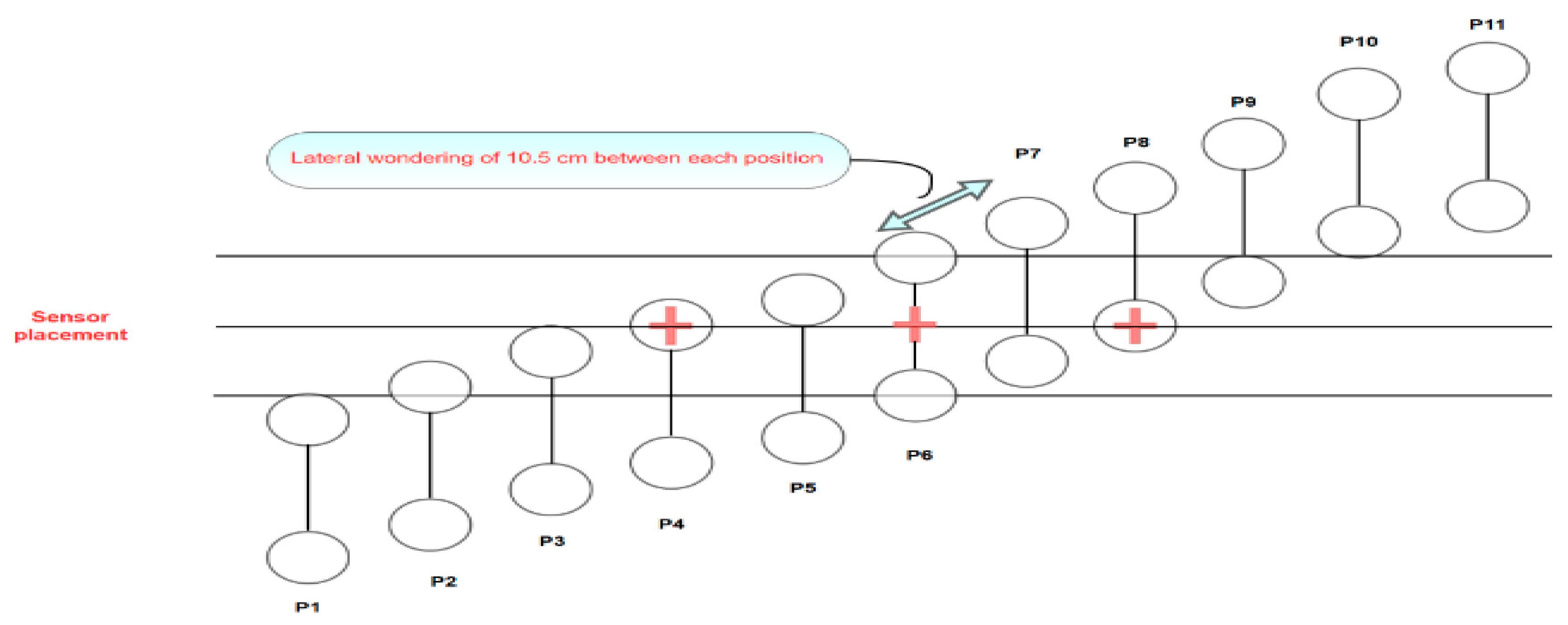
The tests were conducted at different speeds and positions of the wheels with respect to the sensor positions, as shown in
Figure 15. The wheels can move in the transverse direction, over 11 different positions, with a spacing of 10.5 cm. Position 6 corresponds to the central position, where the sensors are placed between the two wheels. For positions 4 and 8, the sensors are placed under the center of one wheel.
6.2. Tests Results
The tests were carried out at three load levels (45, 55, and 65 kN), at speeds varying from 6 m/s to 20 m/s and at surface temperatures of 19 °C to 20 °C. For each test condition, the deflections measured, after signal processing, with the two types of geophones and two types of accelerometers (defined in
Figure 1) were compared with the anchored deflectometer measurements. In this section, in
Figure 16,
Figure 17,
Figure 18 and
Figure 19 the following acronyms are used for the sensors: Geo_ion for Geophone ion, Geo_GS11D for Geophone GS11D, Acc_SD for Accelerometer Silicon Design and ACC_CX for accelerometer CXL04GP1.
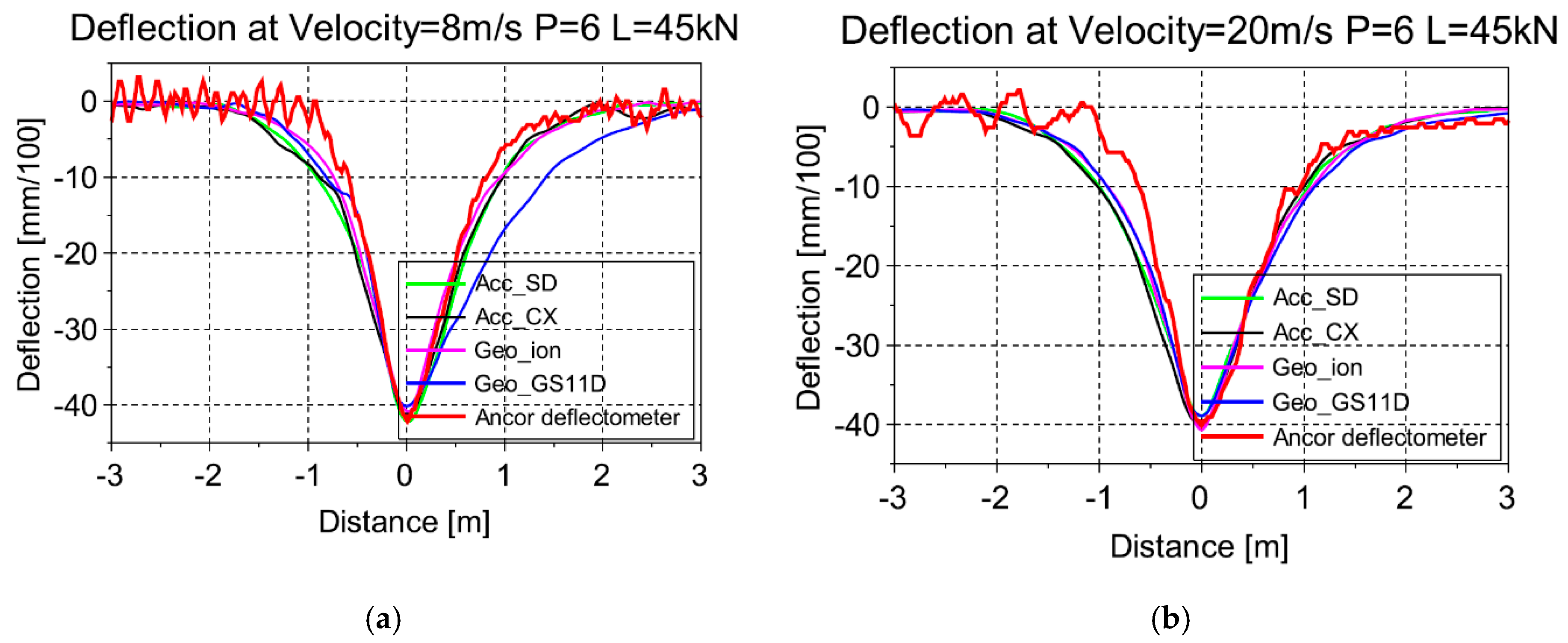
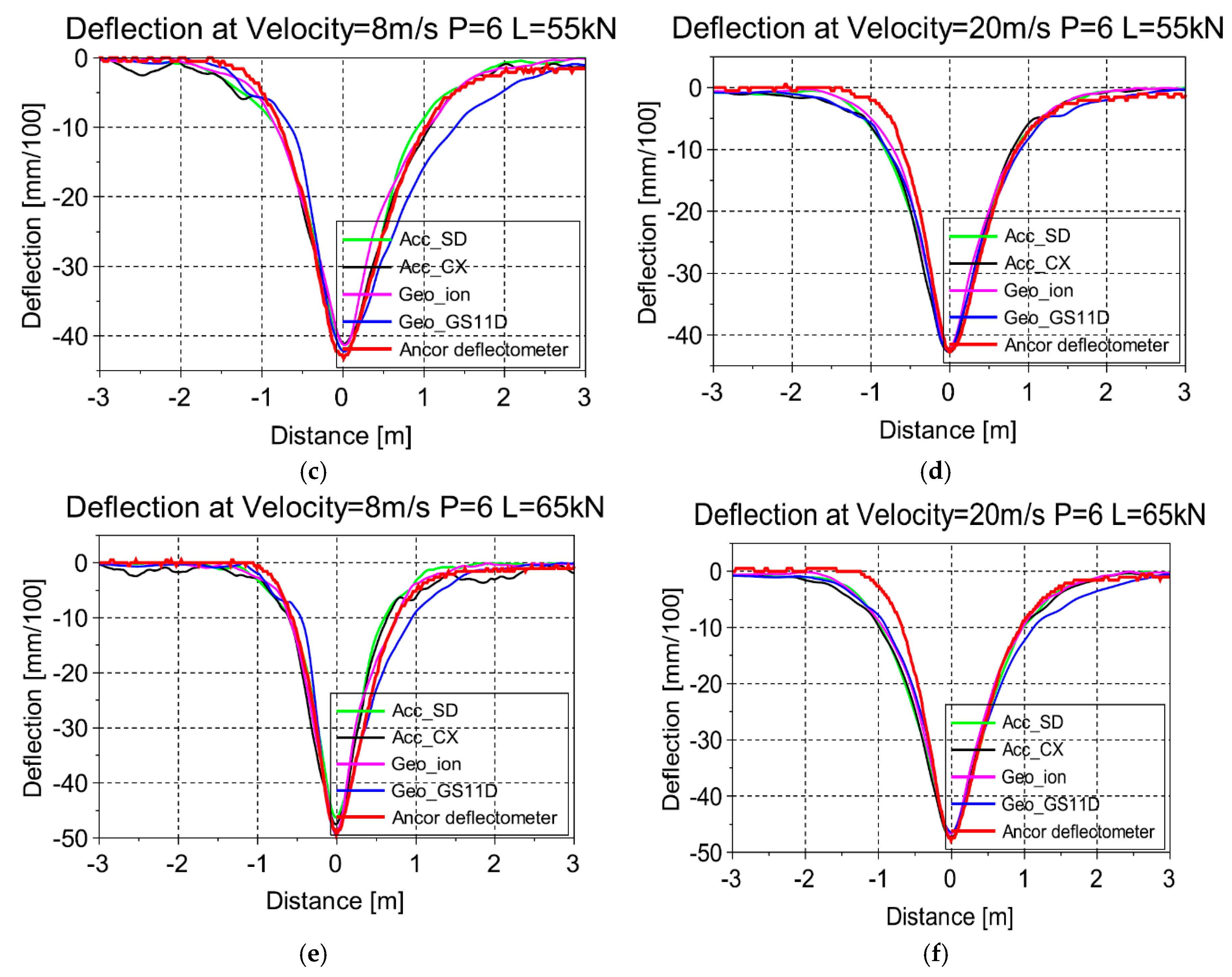
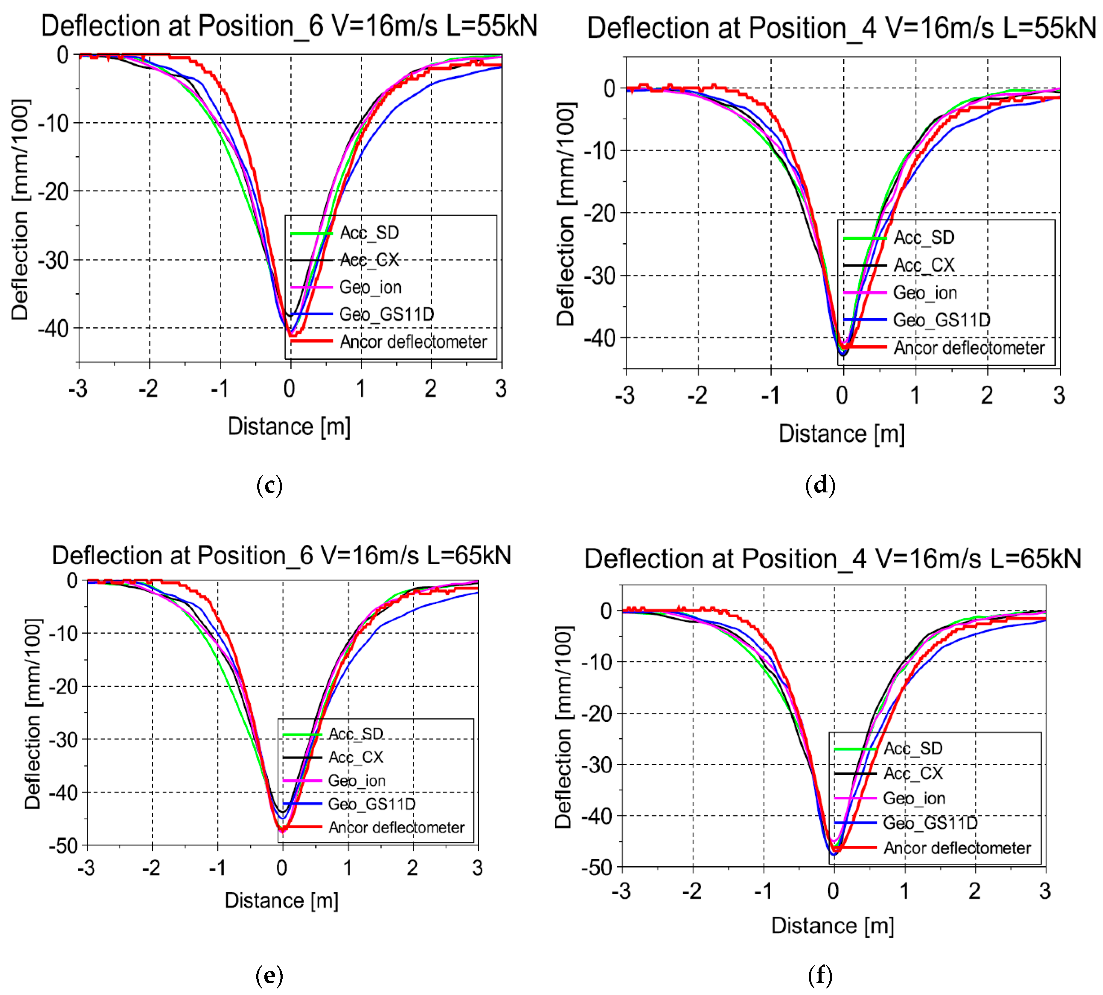
Figure 16 shows the results obtained for speeds of 8 m/s and 20 m/s and position 6 of the wheels.
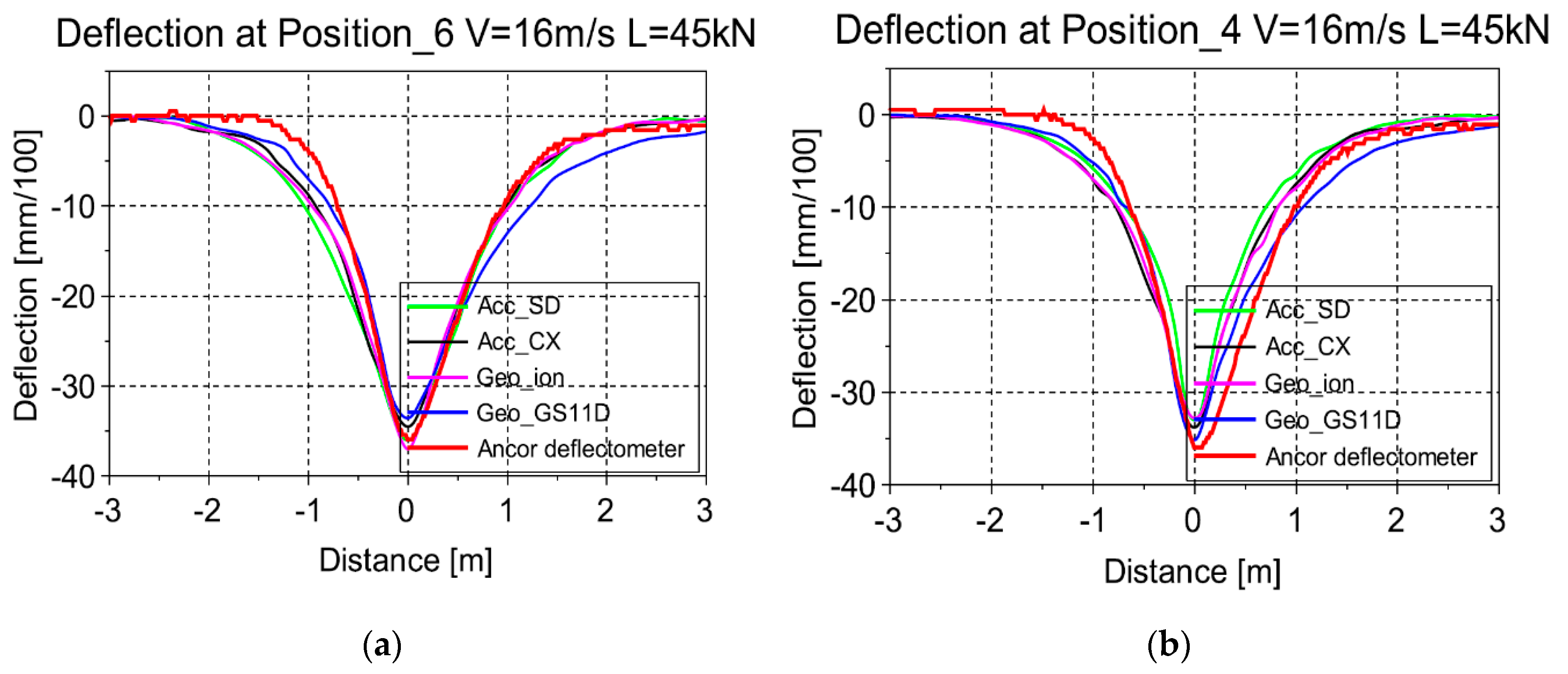
Figure 17 shows the deflection responses corresponding to different lateral positions of the wheels with respect to the sensors. In position 6, the sensors are placed between the wheels whereas, in position 4, the sensors are under the center of one wheel, as shown in
Figure 15. The speed is kept 16 m/s and the maximum deflection is obtained at positions 4 and 6.
The results of
Figure 16 and
Figure 17 show that the deflections obtained with the two geophones and two accelerometers, using the proposed signal processing method, are very close to the reference deflections measured with the deflectometer. The four sensors also give very similar results.
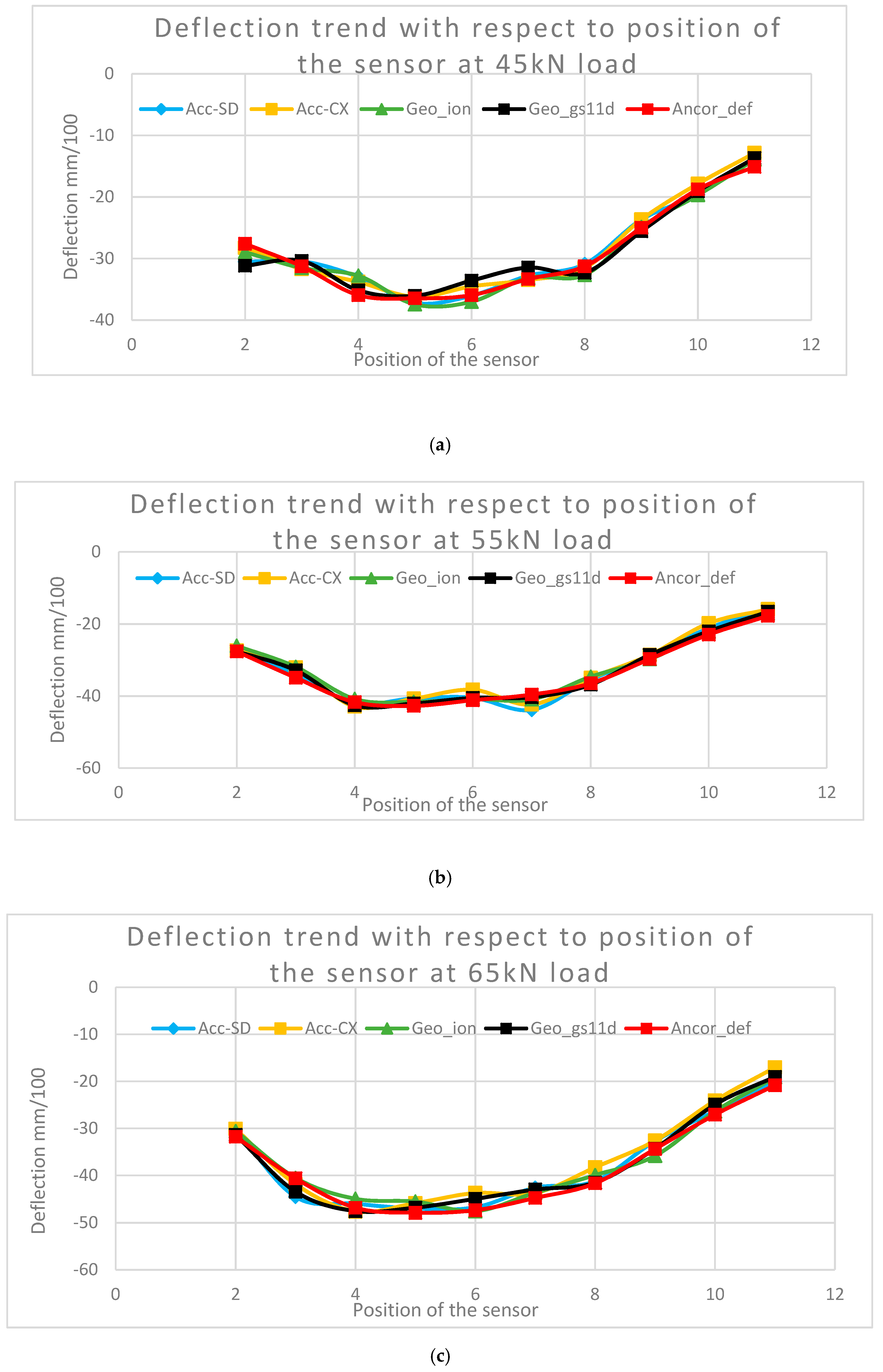
Figure 18 shows the variations of the maximum deflections with increasing speed, from 6 to 20 m/s at position 6. In general, a slight decrease of deflections is observed when the speed increases, except for the speed of 6 m/s, for which the results present more scatter.
Figure 19 shows the variation of the maximum deflections with different wheel positions and a speed of 16 m/s. For all positions, the results obtained with all the sensors are very similar.
To evaluate more precisely the difference between the anchored deflectometer signal, and the signals of the evaluated sensors, an error indicator R was defined. This indicator is expressed by Equation (9). It is defined as the mean relative difference, in percentage, between the values measured by each evaluated sensor and the reference anchored deflectometer, divided by the total number of measurement points N of the signal.
Table 3 summarizes the values of the percentages of difference (error indicator R) obtained between the signals of the geophones and accelerometers, and the signals of the reference anchored deflectometer, for the different test conditions. A mean value of error indicator R is also given for the measurements made for the same load level, and different speeds. This indicator gives an estimate of the accuracy of the measurements for this particular application. It is possible to conclude that:
The error values are relatively low for all the sensors and test conditions (the highest error is 13.7%).
The errors are slightly higher for the 45 kN load level than for the 55 and 65 kN load levels. A possible explanation is that the tests at 45 kN were performed right at the start of the APT test, and that some post compaction, and movement of the transducers may have occurred during these first load cycles and affected the accuracy of the measurements.
For the 55 and 65 kN load levels, mean error values for all the transducers are similar, and very satisfactory (between 3.55% and 5.03%). This validates the original signal treatment procedure used for the calculation of deflections.
7. Data Analysis
7.1. Back Calculation Methodology
The procedure used for the back-calculation of pavement layer moduli is based on the linear elastic pavement design software ALIZE [
12]. This software is used to calculate the response of the experimental pavement (
Table 2) under the APT dual wheel loading, and the corresponding deflection basin. This theoretical deflection basin is then compared with the measured basin, and an iterative method is used to adjust the layer moduli, until the best match between the calculated and measured response is obtained. The methodology used for the optimization of the layer moduli is the following:
The initial characteristics of the pavement (layer thicknesses, initial layer moduli) are entered in Alize
The characteristics of the wheel load are entered in Alize.
The measured deflection basin is discretized into a certain number of points to be inputted in the software
lower and upper limits are defined for the moduli of each layer, for the optimization process (the values used are given in
Table 4).
Successive pavement response calculations are carried out until the best match between the calculated and measured deflections, and thus the best estimate of the pavement layer moduli is obtained.
7.2. Estimation of Pavement Layer Moduli
To evaluate the back-calculation method, measurements made during the APT test at a speed of 20 m/s, a temperature of 19 °C and for position 6 (sensor placement between the wheels) were used. The initial moduli and thicknesses of the pavement layers used for the calculations are defined in
Table 2. The loading considered was the 65 kN dual wheel load of the APT tests. The deflection signals are those presented in
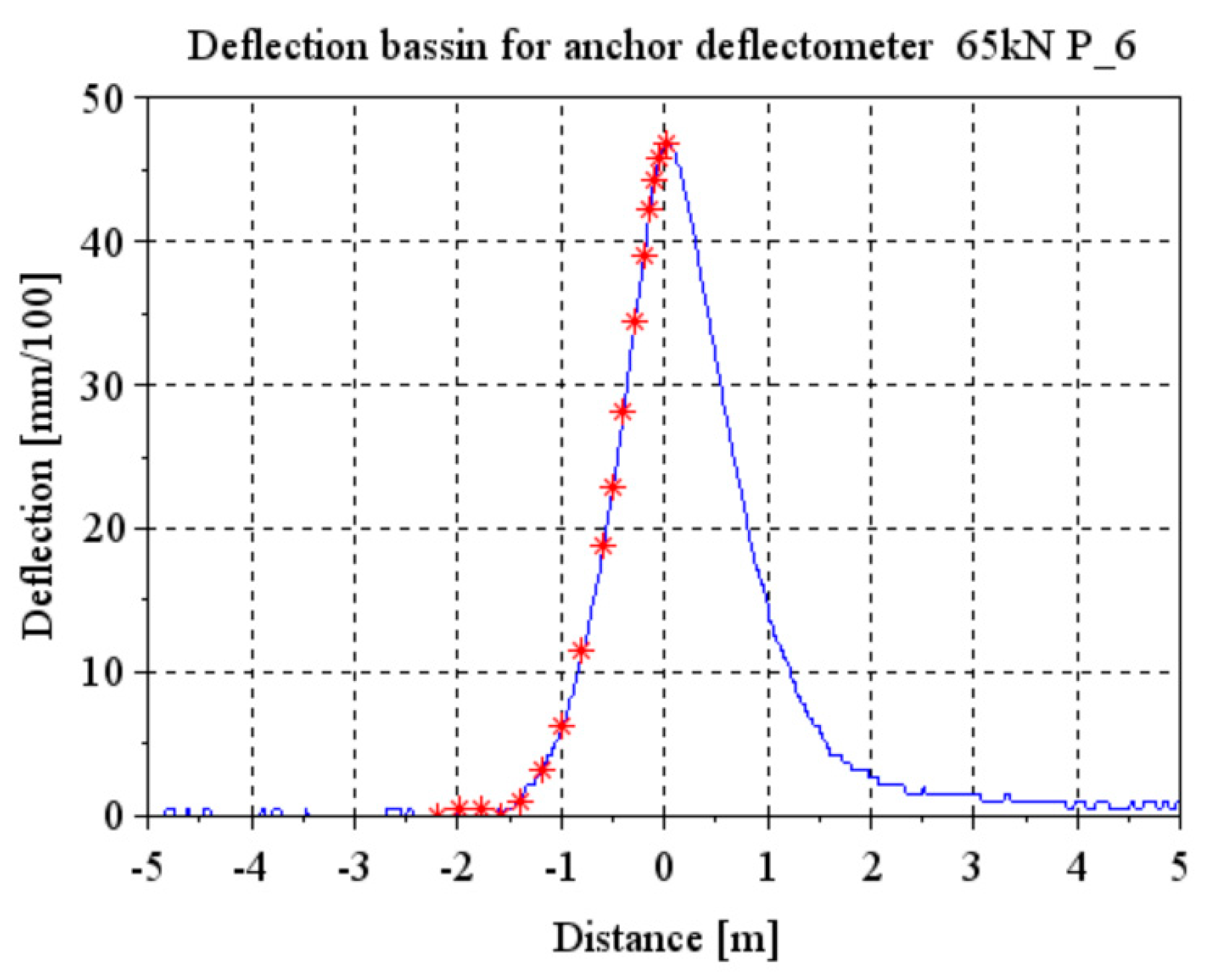
Figure 16. For the back-calculations with Alize, only half of the deflection basins are considered, and the deflection basin of each sensor has been described by a series of points, represented by the red dots in
Figure 20. Points located at the same distance are considered for the geophones and accelerometers, and for the deflectometer. In the calculations, the maximum and minimum attainable modulus values have been limited for each layer, as shown in
Table 4. These limits are needed to facilitate the convergence, and avoid getting unrealistic solutions. The final back-calculated moduli obtained for all the sensors are defined in
Table 5.
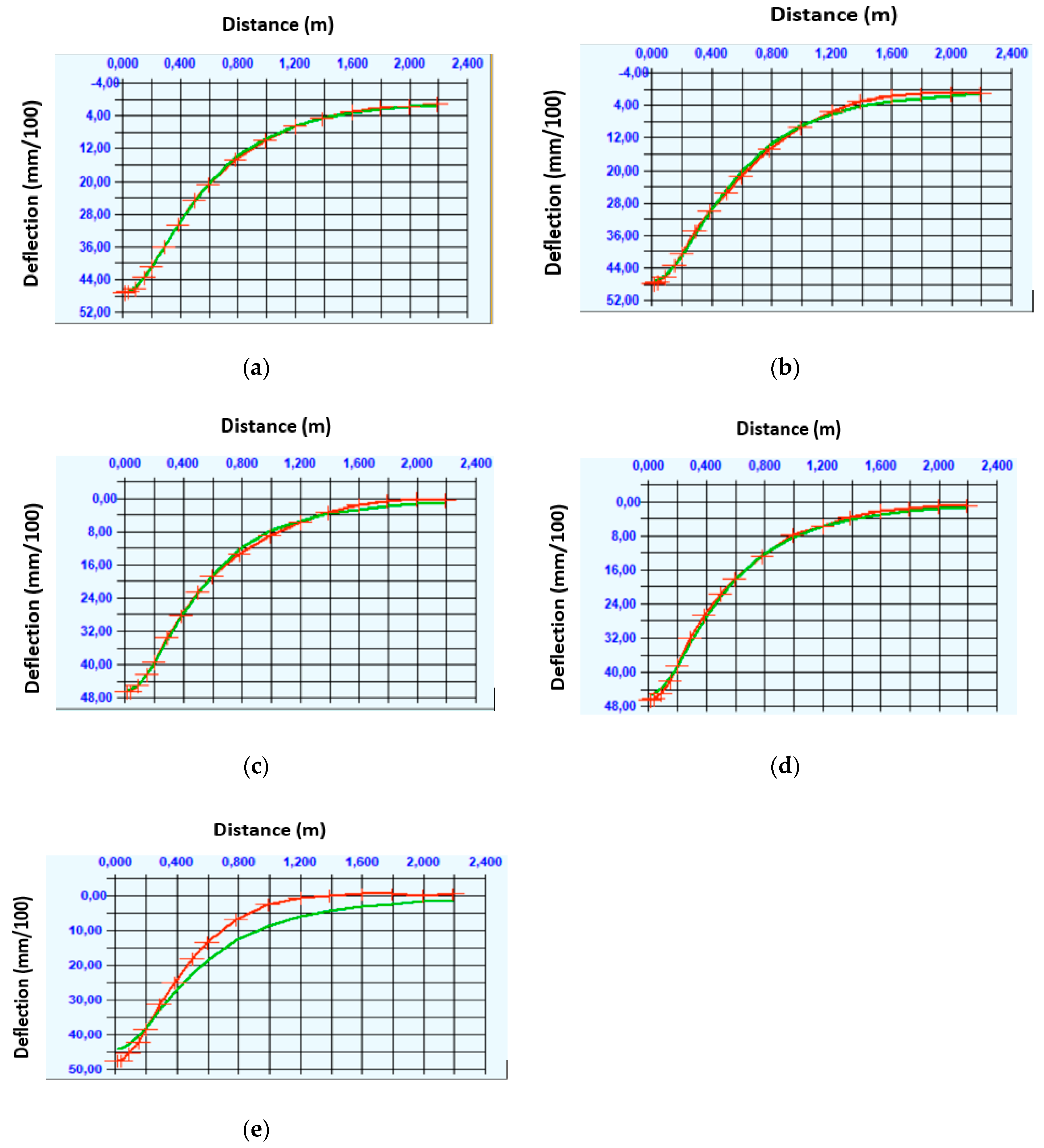
Figure 21a–e represent the fitted deflection basins obtained with Alize, and compare them with the measured deflections. On each figure, the green lines represent the measured values, and the red lines the adjusted calculated deflection curves. For the two geophones and the two accelerometers, a very good fit is obtained between the measured and calculated deflections. For the anchored deflectometer, however, a larger difference between the measured and calculated basin is obtained after the optimization.
The pavement layer moduli back-calculated for each transducer are given in
Table 5, and compared with the reference modulus values obtained previously, from laboratory tests and FWD measurements (
Table 2). In this first example, all the sensors give realistic modulus values, which are close to the reference moduli. For the Asphalt layer modulus, the maximum difference with the reference is about 1400 MPa. For the granular layer and soil, the maximum difference with the reference is 40 MPa. These first results are encouraging, and show that, with the developed signal treatment method, realistic deflection values, and realistic back-calculated moduli can be obtained using the geophones and accelerometers.
8. Conclusions
The most common methods for measuring pavement deflections are dynamic or rolling devices, such as the FWD or deflectograph. However, these methods present some drawbacks: The measurements require to close the road to traffic, and cannot be made continuously. Typically, measurements are made only once every one or two years. The objective of this study was to evaluate an alternative solution for measuring deflections, using embedded sensors. This method offers the possibility to make continuous measurements, under real traffic, and thus to monitor daily and seasonal variations of deflection, and to detect rapidly any pavement deterioration. For this purpose, two types of sensors have been selected: Geophones and accelerometers. These sensors measure respectively the vertical velocity and the vertical acceleration, and deflections can be obtained by a single or double integration of the measurements.
To evaluate the accuracy of deflection measurements obtained with these sensors, two types of accelerometers and two types of geophones have been selected, and tested in the laboratory, on a vibrating table, under simulated pavement deflection signals. The results have shown that a straightforward integration of the results does not give realistic deflection values, but an original signal treatment procedure has been proposed, to correct the measurements. This procedure includes filtering, amplification and integration of the signals, and then application of the Hilbert transform. After this treatment, accurate deflection measurements have been obtained.
In a second step, the sensors have been tested under real moving wheel loading, on the IFSTTAR accelerated pavement testing facility. They have been tested under different test conditions (wheel loads, speeds, and wheel positions). The same signal treatment method has been applied as in the laboratory, and the measurements have been compared with those of an anchored deflectometer, taken as reference. In all cases, a good match has been obtained between deflection values measured with the geophones and accelerometers, and the reference, proving that the four types of sensors are suitable for the measurement of deflections on real pavements. Finally, the deflection basins obtained from the accelerometer and geophone measurements have been used to back-calculate pavement layer moduli, using the Alize pavement design software, which includes a back-calculation tool. Realistic back-calculated moduli have been obtained, indicating that the measured deflection basins are sufficiently accurate to carry this type of analysis, and to monitor pavement layer moduli.
Following this study, it is planned to use the accelerometers and geophones to instrument a real pavement section, to test continuous monitoring of deflections under real road traffic.


