Vision-Based Methodology for Characterizing the Flow of a High-Density Crowd on Footbridges: Strategy and Application

Abstract

Obtaining pedestrian trajectories by a vision-based methodology is receiving increasing attention in the literature over recent decades. Within the field of study of human-induced vibrations on footbridges, practical challenges arise when collecting the trajectories of high-density crowds during measurement campaigns. A cheap and robust methodology tackling these issues is presented and applied on a case study consisting of a real-life footbridge occupied with many pedestrians. A static camera setup consisting of low-cost action cameras with limited installation height is used. In addition, a drone camera was employed to collect a limited amount of footage. Pedestrians are equipped with colored hats and detected using a straightforward color-segmenting approach. The measurements are subjected to both systematic and random measurement errors. The influence of the former is theoretically investigated and is found to be of limited importance. The effect of the latter is minimized using a Kalman filter and smoother. A thorough assessment of the accuracy results reveals that the remaining uncertainty is in the order of magnitude of 2 to 3 cm, which is largely sufficient for the envisaged purpose. Although the methodology is applied on a specific case study in the present work, the conclusions regarding the obtained accuracy and employability are generic since the measurement setup can be extended to a footbridge with virtually any length. Moreover, the empirically obtained results of the presented case study should find use in the calibration of pedestrian dynamic models that describe the flow of high-density crowds on footbridges and the further development of load models describing crowd-induced loading.

1. Introduction

Pedestrian detection is a research field that has known a growing importance over recent time [1]. In particular, the rise of vision-based security applications and the development of driverless cars has stimulated the research effort in this domain e.g., [2,3,4,5,6]. In the field of human-induced vibrations on civil engineering structures, in particular footbridges, an actual need exists for a robust and generic strategy to collect the trajectories of pedestrians in a high-density crowd [7]. Today, state-of-the-art load models describing the complex phenomenon of human-induced loading are developed on laboratory scale [8,9]. Further refinement, validation and calibration of the models is prevented mainly because of the absence of full-scale operational loading data [10,11]. This is in turn a result of the inability to simultaneously collect the induced forces and location of the participants on such a large scale. Besides the further development of the human-induced load models, also the models describing the pedestrian dynamics require validation for the specific case of flows on footbridges [12].

Without influences from the environment, a pedestrian is expected to walk in a straight line in his desired direction. However, the trajectory deviates from a straight line as the result of interaction with other pedestrians (human-human interaction). This phenomenon is shown to have a non-negligible impact on the structural response [12,13]. Several models exist describing these pedestrian dynamics and depending on the situation (uni- versus bi-directional traffic, 1D versus 2D traffic, type of activity, possible presence of obstacles, …), one model provides more realistic flows than the other. Helbing [14] developed a framework describing qualitatively the dynamics of pedestrian flows by a set of coupled differential equations with application-specific parameters. For instance, Refs. [15,16] propose Helbing’s model for evacuation scenarios and validate these based on empirical data. Karamouzas et al. [17] developed a predictive collision avoidance model for the simulation of pedestrian flows. The approach consists of the prediction of future possible collisions with other pedestrians and makes an efficient move to avoid them. van den Berg et al. developed an n-body collision avoidance model that is developed to study the flow of multiple robots avoiding collision among each other [18]. Reynolds [19] developed a framework describing the interaction among individual agents in a group. The original scope of application was to model the flocking behavior of bird-like creatures in animations and gaming applications. A validation of existing pedestrian dynamic models for crowd flows on footbridges is today absent. Only validated pedestrian dynamic models allow the further investigation and development of equivalent, easy-to-use load models for daily engineering practice. Given that the radius of the human body is approximately 30 cm [20], the desired accuracy of the empirical obtained trajectories is set to half of the human body radius (15 cm).

1.1. Related Work

Several attempts so far were made to collect the trajectories during loading of a crowd on footbridges using vision-based methodologies [11,21,22,23,24]. Although general conclusions could be drawn from the collected data, the obtained results are unsatisfying for the actual challenges as not all the pedestrians’ trajectories were captured, the trajectories were swapped, not the entire bridge was covered, the pedestrian density was captured on macro scale, the total duration of observation was too short, the pedestrian density was too low or an extensive manual revision and correction was required. Another practical difficulty often encountered in case of recording footbridges is a suitable setup point of the cameras. High buildings or aerial platforms near the bridge abutments could be used but, keeping in mind that the span of a bridge easily exceeds 50 m, this setup results in a low ground sampling distance and an oblique view at midspan. Therefore, a setup of cameras mounted onto the structure itself using trusses would be a possible solution. The related drawbacks are that the installation height is limited for obvious practical and safety reasons, say, 5 m. Moreover, a large number of cameras will be required given the typical shape of a bridge deck (width in the order of magnitude 2–5 m and total span 20–200 m). To limit the required number of cameras, action cameras can be used as they have a large viewing angle although they possess severe radial distortion.

Successful capturing the motion of pedestrians on small-scale laboratory footbridges is established by tracking visual markers applied on the participants using a commercial motion capture system [25,26,27,28,29]. While the accuracy and the robustness of this system is outstanding, it is not scalable to full-scale outdoor applications because of economical and practical reasons e.g., due to occlusion of the markers in case of high-density crowds. Inspired by these limitations, other approaches were explored such as dead reckoning using inertial sensors [30,31]. Accurate results were obtained, and the scalability seems at first not to be restrained by occlusion. However, the methodology becomes cumbersome for large groups since prior knowledge of the trajectory is required e.g., the entire traveled distance and the principal direction of movement. Localization using dead reckoning can also be performed by smartphones, e.g., [32,33]. Their scope of application lies in the indoor localization in absence of GPS signals. While suited for their intended scope of application, their systematic measurement errors cumulate to errors which are beyond the predefined threshold of 15 cm. The cumulative errors encountered by dead reckoning can be reduced by sensor fusing techniques. Force instance, in [34], a hybrid approach for the indoor localization is proposed which combines the data from the inertial measurement unit with the smartphone camera for the optimal estimation of the location. In [35], the trajectory of a micro aerial vehicle is established combining the inertial measurement unit with a camera that registers markers. While the final accuracy is within the predefined bounds (14 cm), it is impractical for the envisaged scope of application. As the pedestrian would have to walk with their smartphone camera filming their trajectory, it might influence his representative walking behavior. Besides, given the envisaged time duration of the experiments (several hours), the battery life might be a limiting factor.

An alternative approach [36] localizes pedestrians purely based on structural accelerations measured by a network of sensors using wave propagation durations. Despite the fact that the method is advantageous because no additional measurement equipment such as inertial sensors or video cameras are required, the method is inadequate in terms of accuracy (>1 m) and scalability, as footfalls of different pedestrians should not occur simultaneously. The open-source software PeTrack [37] is dedicated to the detection and tracking of pedestrians, both with and without markers. It is successfully used in several pedestrian dynamics calibration applications e.g., [15,38,39,40,41]. The software uses top-view footage of cameras with low to mild radial distortion and detects pedestrians by searching for isolines of the brightness which are nearly ellipsoid. The latter implicit assumption is no longer valid in case of cameras with severe radial distortion e.g., action cameras. Moreover, the developers recognize some robustness issues in case of varying lightning conditions and emphasized the need for a manual revision of the obtained trajectories as some trajectories might be swapped. Given the constraints of the envisaged approach i.e., low camera installation height and as a result a large amount of cameras, outdoor application thus varying lightning conditions, action cameras and thus severe radial distortion and an extreme required robustness given the high number of cameras and test duration, it was opted not to use the PeTrack software but instead develop a custom approach more suited for the application at hand.

1.2. Contribution of the Present Study

This paper starts by presenting a case study of a large-scale measurement campaign where the primary goal was to study the effect of vibrations induced by a high-density crowd on a real-world footbridge. Both walking and jogging activities are considered with a total duration of more than 2 h. A cheap and robust methodology for characterizing the flow of the case study at hand is presented and applied. A static multi-camera setup, using off-the-shelf commercial low-cost cameras, is employed to record the entire bridge deck. The proposed procedure detects pedestrians in the consecutive images independently. Given the artificial circumstances in which the methodology is envisaged to be applied, it is chosen to equip all participants with a colored hat allowing an easy detection using color segmentation while little a priori knowledge of the scene is required. Image-plane measurements are converted to corresponding world coordinates considering both mono and stereo-view setups. Finally, the detections are assigned to their corresponding trajectories while the influence of the inevitable random measurement noise is mitigated using a Kalman filter. Since the results are processed offline, the state uncertainty is further reduced by applying a smoother. Besides the random noise, there is also a systematic source of error as a result deformation of the non-spherical shape of the hat in case of projection and the vertical sway of the head during the locomotion of the participant. The accuracy of obtained trajectories is investigated and assessed with respect to the predefined threshold of 15 cm. Besides the static camera setup, a limited amount of footage was collected using a drone. While the data is insufficient to reconstruct the trajectories on the entire bridge deck, it allows an assessment of the accuracy. Given their ease of use, short setup time and flexibility, drones have the potential to become the preferred data acquisition system when applied within the context of structural dynamic measurement campaigns involving the registration of the participants’ trajectories. The results of this case study should find use in (1) the calibration of pedestrian dynamic models for flows on footbridges and (2) the further development of load models that describe crowd-induced loading on footbridges.

The authors published a previous study [42] dealing with the characterization of a high-density flow based on the footage recorded during a large-scale measurement campaign (142 participants, 1.0 pers./m²). While the present study is founded on the same philosophy, it contains some major improvements and novel contributions which are summarized as follows:

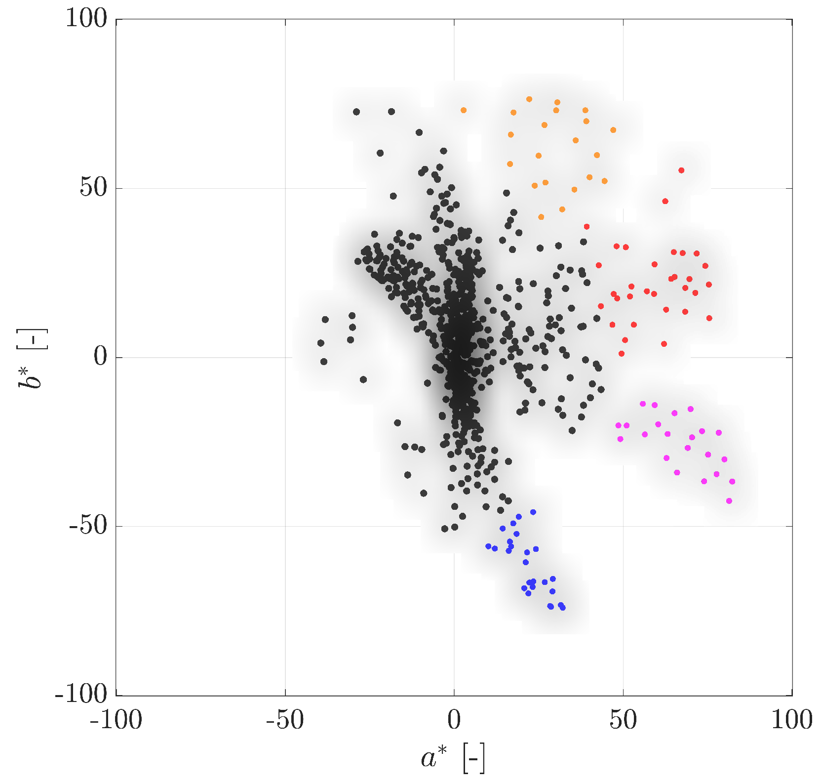
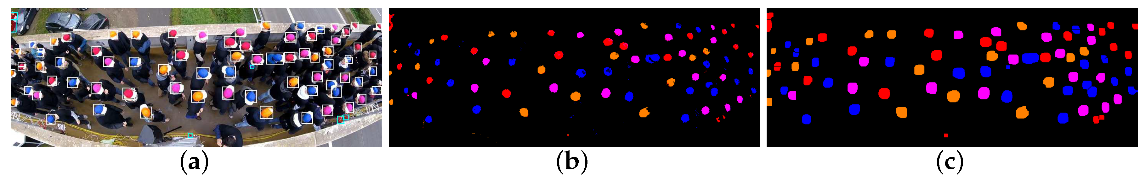
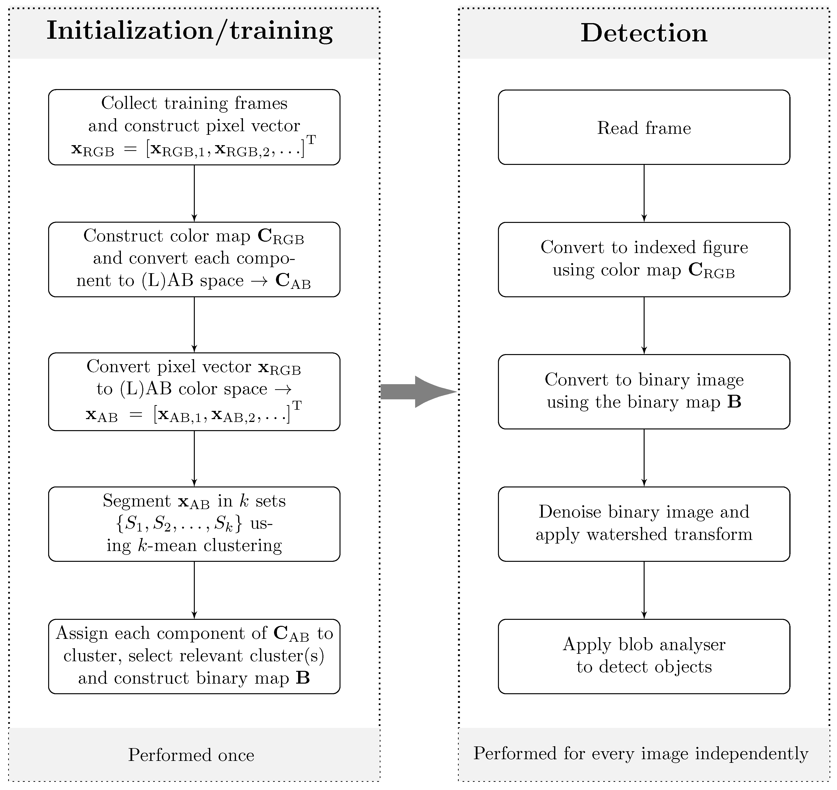
• A computationally efficient approach to detect the pedestrians is proposed employing image indexing by a limited number of colors. A detection map for the colors corresponding to the detection is only initialized a single time using a vector quantization algorithm which greatly enhances the processing speed.
• An approach is proposed to minimize the influence of the random measurement noise. To this extent, a Kalman filter and smoother are applied thereby maximally exploiting the fact that the results are processed offline instead of online. Its optimal characteristics are determined using an expectation maximizing algorithm. The methodology in [42] only used a Kalman filter where its parameters were chosen using engineering judgment.
• An overview of the present systematic measurement errors in the envisaged scope of applications is presented and its effect on the obtained trajectories is evaluated.
• The methodology is applied on a benchmark data set yielding the time-variant positions of all the participants which constitutes an indispensable quantity for the benchmark data set. Moreover, the time duration is now much longer (>2 h instead of 10 min).
• The considered activities now comprise both walking and jogging events instead of only walking events.
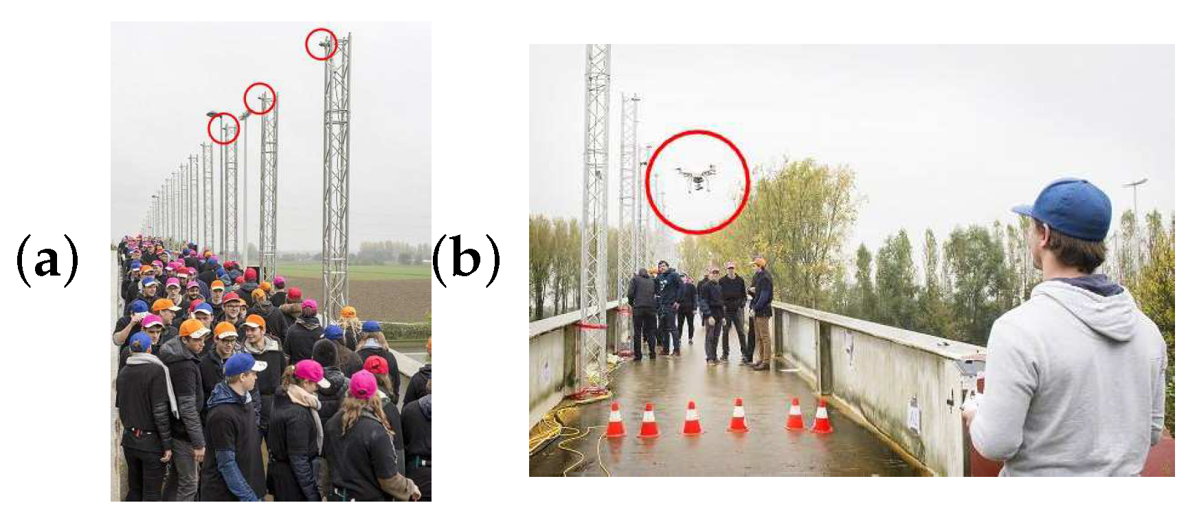
• Besides a static camera setup, additional footage captured by a drone is now considered as well.

The remainder of the paper is organized as follows. A description of the measurement campaign (Section 2) is followed by the detection methodology (Section 3). Next, the mono and stereo camera setups and their respective conversion of coordinates from the image plane to world space, including an assessment of the related accuracy is presented (Section 4). The results are shown and discussed in Section 5 and followed by summarizing the most important conclusions (Section 6).

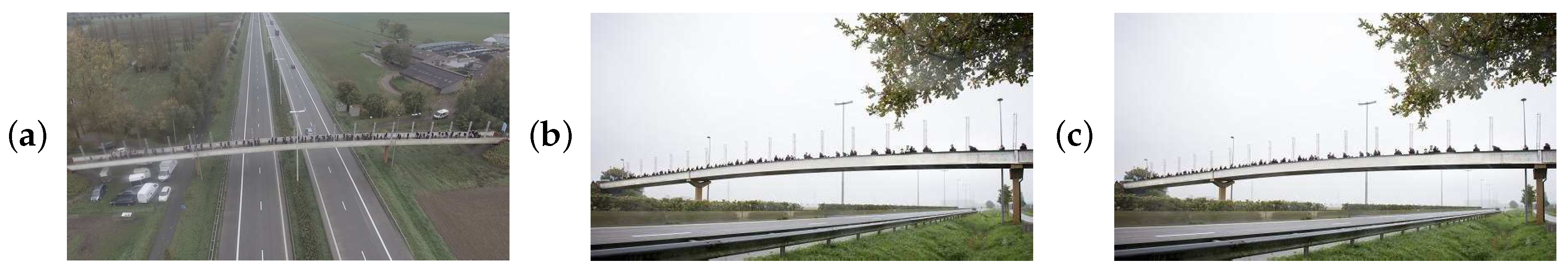
2. Large-Scale Measurement Campaign

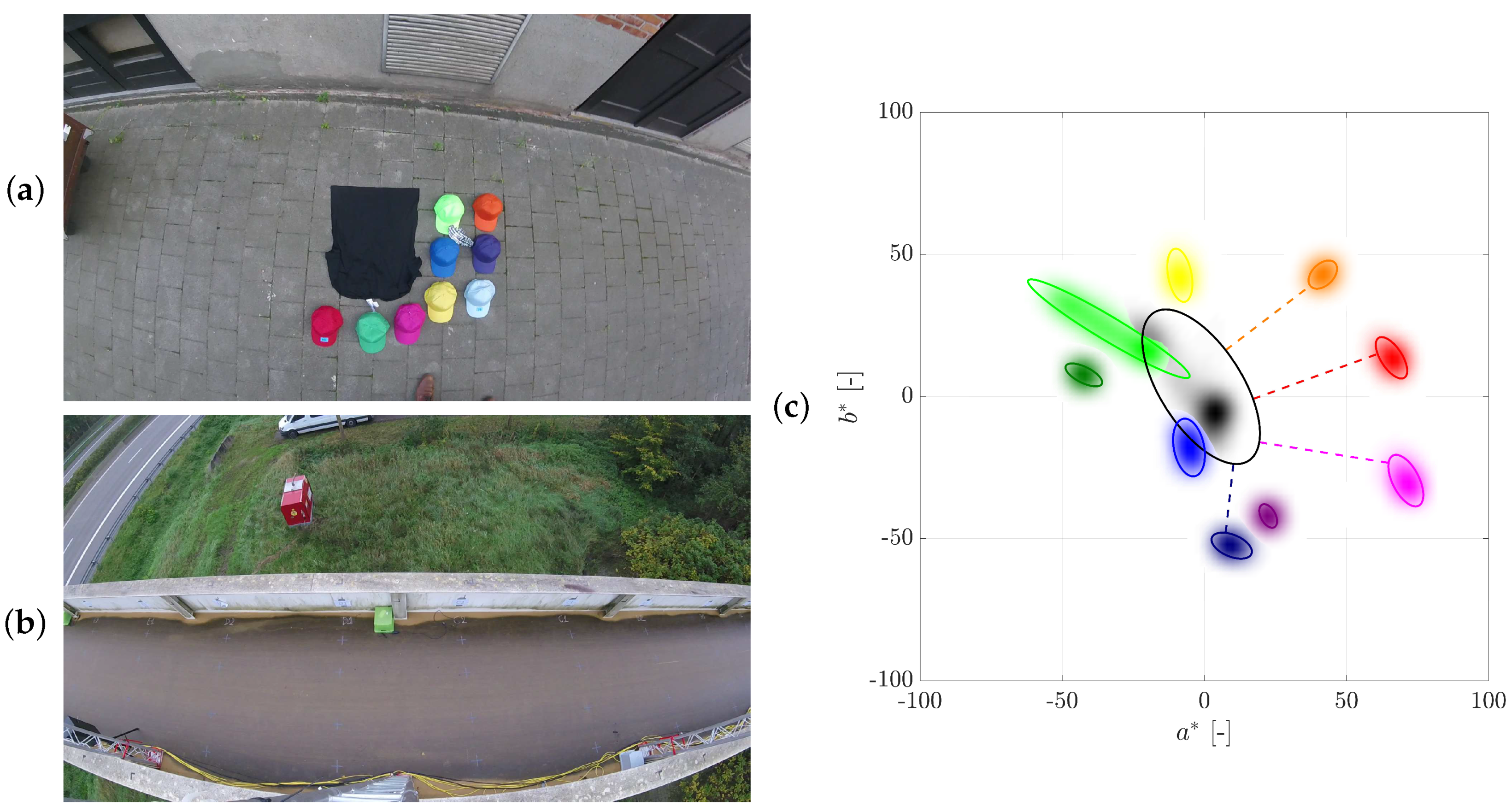
A large-scale measurement campaign was performed involving several types of human loading (walking and jogging,

Table 1. Overview of events: name, activity, number of participants, duration and number of video frames recorded by the static camera setup.

Test Number	Activity	Number of Participants [-]	Duration [s]	No. of Frames [K]
1	Jogging	15	800	504
2	Jogging	15	900	567
3	Jogging	15	300	189
4	Walking	73	720	454
5	Walking	73	315	199
6	Walking	73	660	416
7	Walking	73	649	409
8	Walking	72	1860	1172
9	Walking	148	1200	756
10	Walking	148	1200	756
11	Walking	148	950	599
12	Walking	148	300	189
13	Jogging	74	400	252

). The considered footbridge consists of one main (arc-shaped) and two side (straight) spans and has a total length of 96 m and a width of 3 m. A more comprehensive description of the architecture and the dynamical characteristics is found in [43]. An impression of the structure during the large-scale measurement campaign is shown in Figure 1. Different pedestrian densities were considered, with a total of 148 persons corresponding to a density of 0.50 pers./m². All tests were approved by the ethical committee of KU Leuven and all participants signed an informed consent prior to the measurement campaign. One of the principal objectives was to obtain the trajectories of every single pedestrian. Besides the trajectories, the structural accelerations are measured at 15 locations along the bridge deck using triaxial wireless Geosig recorders. The 3D body motion of all 148 persons was captured using an individual inertial motion sensor during the entire campaign. The combined in-field motion information (2D trajectories and 3D body motion) can be used to characterize the forces induced by the crowd [43]. The simultaneous registration of the input (induced forces) and output (accelerations) provides a unique state-of-the-art benchmark data set within the field of human-induced vibrations on footbridges. Every participant is given a participant number which is used for the coupling with the registered body motion and anonymized in the further process. The bridge was closed the entire day to the public and as such no coincidental passers-by are recorded by the camera network thereby avoiding potential privacy issues.

2.1. Camera Setup

Twenty-one static cameras (GoPro, Hero Session, 1080p, 30 fps) were used to register the entire bridge deck. The devices were mounted on aluminum trusses which were firmly fixed to the parapet the bridge deck. The position of the static cameras and the global axes considered in the present study are shown in Figure 2. The cameras were synchronized offline, using a common occurrence in the different cameras, i.e., a car driving with a speed of approximately 120 km/h crossing a reference point. As the car speed is high compared to the walking speed of the pedestrians (≈5 km/h) and the given frame rate, the synchronization of the frames is more than sufficient. Figure 3 shows an example of 3 synchronized images. The duration and number of video frames as recored by the static camera setup for each test is listed in Table 1.

Additionally to the static camera setup a drone (DJI, Phantom 3, 2.7K, 30 fps) was used. Due to the higher resolution and the unconstrained location of the camera, the drone has the major advantage that fewer cameras are needed to record the entire bridge deck and that the setup time is much lower. In the current campaign, however, only a single drone partially registering the bridge deck was used as a proof of concept. Both the static camera setup and drone are shown in Figure 4.

The camera locations are the result of an economical-practical constrained optimization problem. Pedestrians’ hats should not be occluded while the average ground sampling distance should be sufficiently high for the hats to be detectable. In case of the static cameras, the installation position cannot be too high due to practical installation constraints. The field of view (FOV) for both camera setups is calculated assuming a rectangular grid of pedestrians with a minimal distance of 75 cm (i.e., 2.5 times the body radius). The pedestrian’s height is assigned a uniformly distributed random value between 1.6 m and 2.0 m while the colored hat is represented by a hemisphere with a radius of 10 cm [20]. It is opted to place a static camera at every transverse stiffener of the bridge deck (interdistance of 4.5 m or 4.2 m). The cameras are mounted at a height of 5 m and a view direction of 170 degrees with the vertical axis. The drone’s 3D location is chosen at a quarter of the bridge deck length in X direction, half a bridge deck in the Y direction, a height of 18 m and a view direction that coincides with the downward vertical direction. The simulated situation is shown in Figure 5a. The calculated FOV of a static camera and the drone (Figure 5b,c) indicate that this setup leads to an unoccluded view of the hats for the given assumptions. The average ground sampling distance at the bridge deck is in the order of magnitude of 6 mm/pix and 3 mm/pix for the static and drone camera, respectively. Given that the radius of the colored hat is approximately 10 cm, the ground sampling distance is sufficient to allow a detection of the hats in the image planes. The exact location and orientation during the measurement campaign of the recording devices is obtained by a calibration procedure (Section 4.1.2). Strictly speaking, one only needs 10 cameras (corresponding to the odd numbers in Figure 5a) to capture the entire bridge deck since the FOV is wide enough. In the present study, 21 cameras are used, however. The additional cameras serve as a redundant measure in case one of the cameras would drop out as a result of power loss. Moreover, the current camera setup corresponds to a situation where every point on the bridge deck is recorded by two devices, hence allowing a stereo vision which is more accurate than mono-vision. The availability of stereo vision allows assessment of the accuracy of the tracks that are obtained by the mono-vision setup.

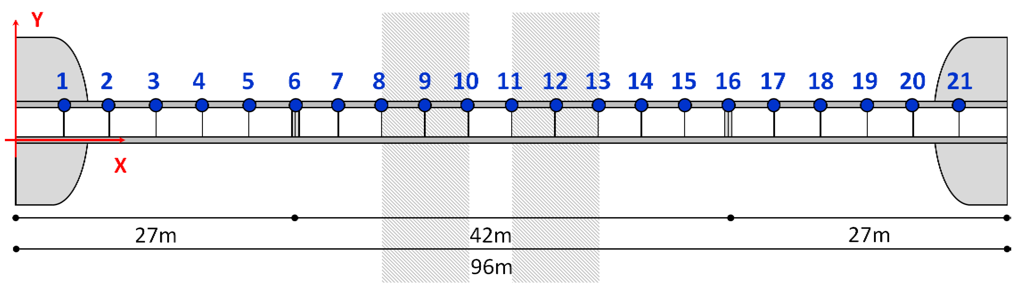
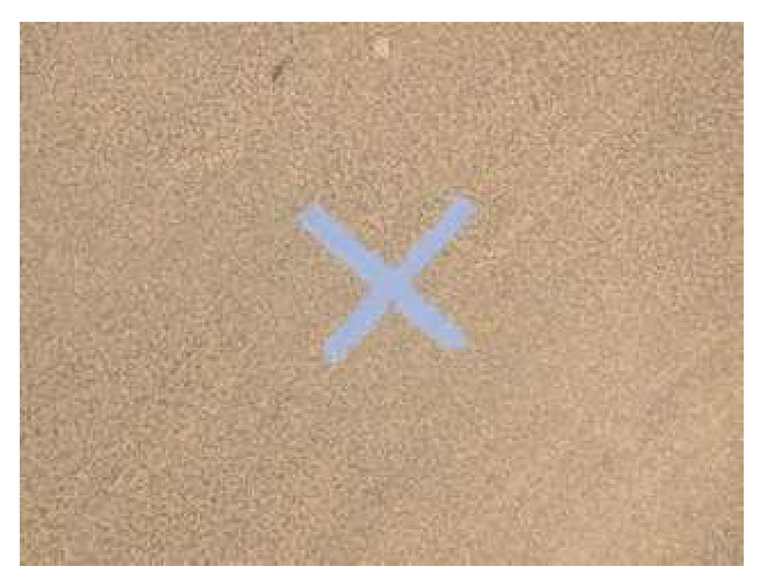
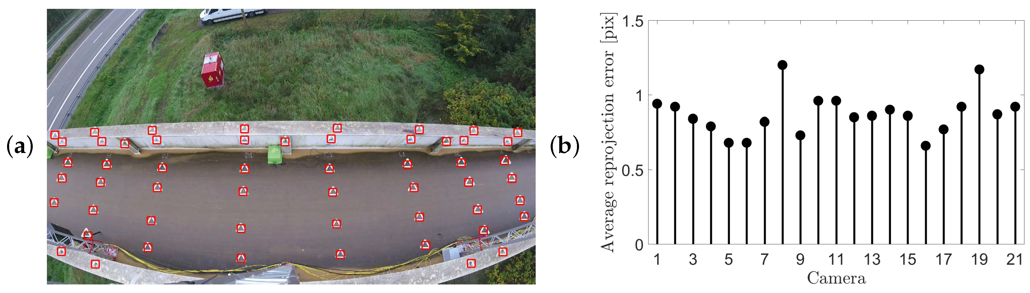
2.2. Calibration Points

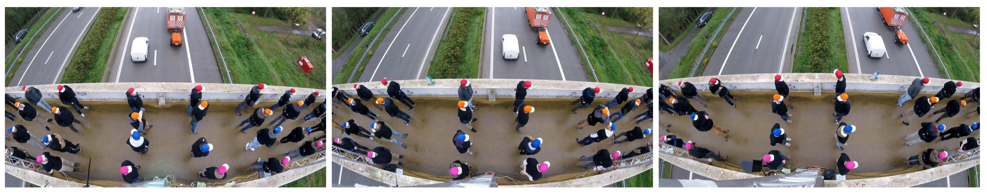
All cameras are calibrated using a set of 2D-3D correspondences [44]. To this end, ×-shaped symbols were indicated with a paint marker (standard deviation signal marker location: 2 mm) on the bridge deck (Figure 6), making them easily recognizable and uniquely identifiable in the images. Their world position was measured using a total station (standard deviation measurement error: 1 mm). The collection of 331 calibration points comprises 176 marks on the bridge deck, 23 on the transverse stiffeners, 44 on the web plate of the parapet and 88 points on top of the parapet.

2.3. Colored Hats

All pedestrians were equipped with colored hats to easily detect them using a color-segmentation algorithm (Section 3). The trajectory of every single pedestrian is to be coupled with a corresponding inertial sensor unit measurement and therefore every pedestrian was assigned a start and stop zone. To facilitate the association procedure, the number of pedestrians in each start and stop zone was limited to four, all with a different color such that the pedestrians are clearly distinguishable.

In the present work, all color-related analyses are done in the CIELAB color space [45]. The conversion is non-linear but reversible and is designed to be independent of the device. The RGB value of a pixel (as recorded by the camera) is decoupled into the triplet $(L,a^{*},b^{*})$, where L represents the illumination while $a^{*}$ and $b^{*}$ are the green-red and blue-yellow color information. The illumination L is disregarded in the further analysis.

To select four optimal hat colors available from the supplier, a preliminary study was performed. Pictures were made of the candidate hat colors (light green, dark green, light blue, dark blue, yellow, purple, magenta, orange and red) and the background. Their corresponding ($a^{*}$,$b^{*}$) coordinates are plotted in Figure 7. Based on the latter representation, it was opted to use the red, orange, dark blue and magenta colors in the measurement campaign. The distance in the ($a^{*}$,$b^{*}$)-plane is maximal to the background while their interdistance is sufficient to be distinguishable.

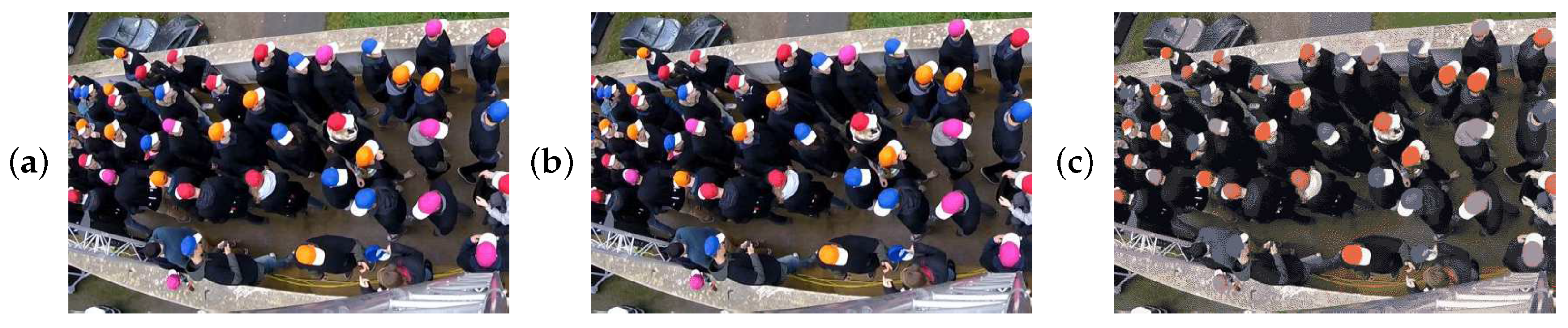
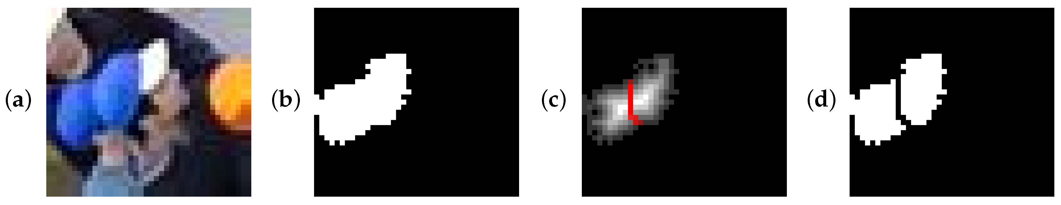
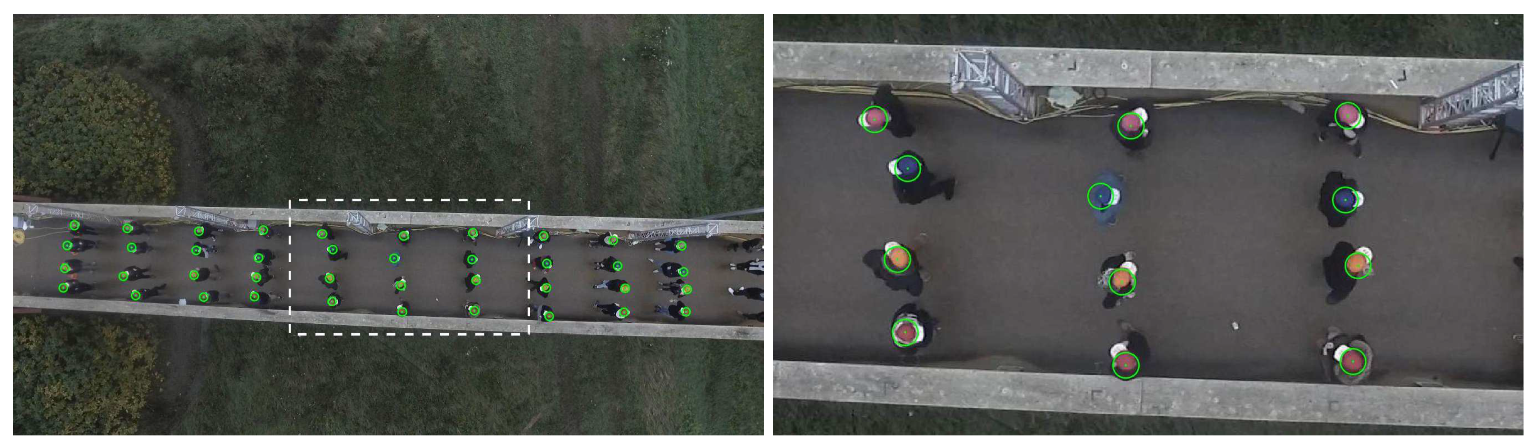
3. Pedestrian Detection

The use of colored hats facilitates a straightforward detection by color segmentation of the images, resulting in 4 binary images with values 1 (detection) and 0 (background), one for each of the chosen colors. The procedures described in Section 3 and Section 4 employ various functions of the Computer Vision Toolbox of Matlab R2016b [46].

Every pixel consists of three unsigned bytes (value range: 0–255) yielding 256³ (16,777,216) possible values. Since the purpose is to segment the images, such degree of detail of color information is not required and results in computational-costly operations. Therefore, the images are converted to indexed images, only retaining a certain number of colors $n_{\mathrm{color}}$, stored in a color map ${\mathbf{C}}_{\mathrm{RGB}}$. The image is encoded such that every pixel is assigned one color of ${\mathbf{C}}_{\mathrm{RGB}}$. This procedure is a form of vector quantization compression and speeds up the performance of the image processing while saving computer memory. First, a set of 50 training frames is selected, involving all cameras and varying illumination conditions. The pixels of all training frames are stored in the vector ${\mathbf{x}}_{\mathrm{RGB}}$. Next, a color map ${\mathbf{C}}_{\mathrm{RGB}}$ is defined using a minimum variance quantization method, as proposed in [47] (function rgb2ind). The method accounts for the actual input, ${\mathbf{x}}_{\mathrm{RGB}}$, and allocates the elements of the color map ${\mathbf{C}}_{\mathrm{RGB}}$ according to the spatial distribution of the elements in ${\mathbf{x}}_{\mathrm{RGB}}$. The procedure is illustrated for an image in Figure 8 where only a fraction of the 256³ colors is retained. In the further analysis, the number of elements in the color map is set to 1000 as the experiments showed that this number retains sufficient color information to perform a color-segmentation process yet greatly increases the processing speed.

Next, both the pixel vector ${\mathbf{x}}_{\mathrm{RGB}}$ and corresponding color map ${\mathbf{C}}_{\mathrm{RGB}}$ are converted to the (L)AB space yielding the quantities ${\mathbf{x}}_{\mathrm{AB}}$ and ${\mathbf{C}}_{\mathrm{AB}}$. To determine which elements of ${\mathbf{C}}_{\mathrm{AB}}$ belong to the background or a detected color, the vector is segmented into k clusters using k-means clustering [48]. This algorithm assigns every element of ${\mathbf{C}}_{\mathrm{AB}}$ into one of the k sets $\mathbf{S}=(S_1,S_2,\dots ,S_k)$ such that the within-cluster sum of squares is minimized:

$$\underset{\mathbf{S}}{arg\; min}\sum _{i=1}^k\sum _{{\mathbf{x}}_{\mathrm{AB},j}\in S_i}\left|\right|{\mathbf{x}}_{\mathrm{AB},j}-{\mu }_i{\left|\right|}^2$$

(1)

where ${\mu }_i$ is the mean of the points in subset $S_i$ (function kmeans).

The present work uses 10 clusters to segment the colors. The clusters matching the colors of the hat are selected, thereby defining the corresponding regions in the $(a^{*},b^{*})$ space. As the mapping of the RGB to the CIELAB color space is one-to-one, each component of ${\mathbf{C}}_{\mathrm{RGB}}$ can thus, via the corresponding component in the vector ${\mathbf{C}}_{\mathrm{AB}}$, be related to a binary value. Because four hat colors are used, the final result is four binary maps ${\mathbf{B}}_{\mathrm{red}}$, ${\mathbf{B}}_{\mathrm{orange}}$, ${\mathbf{B}}_{\mathrm{blue}}$ and ${\mathbf{B}}_{\mathrm{magenta}}$, which are practically combined to a single binary map $\mathbf{B}$. Figure 9 shows the results of the applied procedure.

The process of converting a RGB image to a binary image now boils down to converting the RGB frame to an indexed image using the standard reduced RGB color map ${\mathbf{C}}_{\mathrm{RGB}}$ and reconverting it to a binary image using the binary map $\mathbf{B}$.

The remaining spurious pixels in the obtained binary images are removed by consecutively applying several morphological operations. An image erosion with a disk of radius 5 pixels is followed by a flood-fill operation. Next, the frame is dilated using a disk with radius 5 pixels followed by a morphological opening (i.e., dilation followed by an erosion) of the binary image with the same structural element as the first time. Practically, the functions imerode, imfill, imdilate and imopen are used. A blob analysis (function blobAnalyzer) is applied on the binary image, resulting in a selection of the center of gravity of the blobs whose area exceeds a user-defined threshold (30 pixels, corresponding with a ground area of approximately 11 cm², Section 2.1). Figure 10 shows an example of the color segmentation, the morphological operations and object detection procedure. The order of operations and morphological parameters were chosen by trial-and-error such that the recall is 100% (i.e., there are no false negatives), even if the consequence is that the precision is lower than 100% (i.e., there might be false positives). If closely investigated, one can observe that the final results indeed yield some misdetections (Figure 10a). These false positives typically occur when participants wear clothes which have the same color as the predefined hats. Also, some fixed objects visible in the frames give rise to false detections e.g., the red ribbon which is used to fix the truss to the bridge. The incorrect detections are removed in the data association step (Section 4).

One important drawback of the color-segmentation algorithm is that two adjacent blob regions of the same color can be incorrectly joined (Figure 11a,b). This occurs most often at the outer sides of the FOV of the cameras because of the increased obliqueness and for two pedestrians with a small interdistance (<75 cm) and a large difference in height. To overcome this issue, a watershed analysis (function watershed) is performed. This transform is often used in the field of image processing for segmentation purposes and defined on a grayscale image [49]. When the gray value is thought of as a topographic quantity, the watershed returns the lines which correspond with the ridges of this quantity. In the present case, the binary distance (function bwdist) of a pixel is considered to be the relevant property, defined as the maximum horizontal or vertical distance of a certain pixel to the nearest pixel which has the value zero [50]. As the detection of a hat is typically nearly discoid, two adjacent circles possess a local ridge in the binary distance. As such, a watershed transform allows segmentation of these bounded regions into two disjoint ones. An illustration of the use of the watershed process to segment two adjacent blobs initially detected as one is shown in Figure 11.

The detection algorithm is performed on a desktop computer with an Intel Xeon E5-2630 @ 2.4 GHz quad core processor using Windows 10 Enterprise x64 with 144 GB of RAM. The process is computed in parallel on 12 subgroups. Every image is processed offline and independently. The required wall-clock time of each frame is approximately 200 ms, with relative time durations of 1% to read the frame, 1% to index it, 3% to create the binary mask, 78% for the denoising operations, 16% for the application of the watershed analysis and 1% for the blob analysis.

The pedestrian detection using color segmentation is summarized in a flow chart (Figure 12).

4. Pedestrian Trajectory Reconstruction

Once the pedestrians are detected in the different frames independently, the challenge lies in reconstructing the trajectory of a certain pedestrian across the different recording devices and consecutive frames. Furthermore, the obtained detections must be converted to world coordinates. Moreover, misdetections are present and can lead to erroneous results when wrongly assigned. In addition, even if a correct assignment is made, the measurement is subject to an error, both random and systematic. An overview of the methods employed to convert the obtained image detections to corresponding world coordinates is presented. The effect of the random and systematic measurement error is evaluated and a Kalman filter and smoother are implemented to minimize the effect of the random measurement error.

4.1. Transformation of 2D Image Coordinates to 3D World Coordinates

4.1.1. Camera Model

The standard pinhole camera model [51] relates a world point $\mathbf{M}={[X,Y,Z,W]}^{\mathrm{T}}$ to a corresponding image point $\mathbf{m}={[x,y,w]}^{\mathrm{T}}$, both expressed in homogeneous coordinates. In the case of Euclidean coordinates, the last component i.e., W or w equals 1. The projection is described by Equation (3) where ≃ means “equal up to a non-zero scale factor”:

$$\begin{array}{cc}\hfill \mathbf{m}& \simeq \mathbf{P}\mathbf{M}\hfill \end{array}$$

(2)

$$\begin{array}{cc}\hfill \mathbf{m}& \simeq \mathbf{K}\left[{\mathbf{R}}^T\right|-{\mathbf{R}}^T\mathbf{t}]\mathbf{M}\hfill \end{array}$$

(3)

with $\mathbf{P}$ the projection matrix and $\mathbf{K}$ the matrix describing the intrinsic parameters of the camera:

$$\mathbf{K}=\left[\begin{array}{ccc}{\alpha }_{\mathrm{x}}& s& u_{\mathrm{x}}\\ 0& {\alpha }_{\mathrm{y}}& u_{\mathrm{y}}\\ 0& 0& 1\end{array}\right]$$

(4)

with ${\alpha }_{\mathrm{x}}$ and ${\alpha }_{\mathrm{y}}$ the focal length, expressed in pixels, s the skew and $u_{\mathrm{x}}$ and $u_{\mathrm{y}}$ the location of the principal point, expressed in pixel coordinates. As digital cameras do not possess any skew, it holds that $s=0$.

$\mathbf{R}$ and $\mathbf{t}={[t_X,t_Y,t_Z]}^{\mathrm{T}}$ are a 3 × 3 matrix and 3 × 1 vector respectively, describing the orientation and position of the camera in world coordinates. While the rotation matrix $\mathbf{R}$ is a $3\times 3$ matrix, it has only three degrees of freedom and can expressed in terms of its Euler angles: ${[{\theta }_{\mathrm{X}},{\theta }_{\mathrm{Y}},{\theta }_{\mathrm{Z}}]}^{\mathrm{T}}$. The projection matrix $\mathbf{P}$ is 3 × 4.

Equation (3) is a linear equation and is an idealization of the actual projection mechanism of real-life cameras. The linear model does not capture radial or tangential distortion effects, typically present in such cameras. As the influence of tangential distortion is usually much smaller than radial distortion, only the latter effect is taken into account. The effect is modeled by a function describing the relation of the distorted and undistorted coordinates in the focal plane. The function is a polynomial where the first constant is zero (i.e., there is no constant term in the relation) and the three consecutive coefficients denoted as $[{\kappa }_1,{\kappa }_2,{\kappa }_3]$. Consequently, the relation between the image point $\mathbf{m}$ and the world point $\mathbf{M}$ becomes non-linear and is denoted by the vector function F:

$$\mathbf{m}=F({\mathbf{x}}_{\mathrm{cam}},\mathbf{M})$$

(5)

with ${\mathbf{x}}_{\mathrm{cam}}={[{\alpha }_{\mathrm{x}},{\alpha }_{\mathrm{y}},u_{\mathrm{x}},u_{\mathrm{y}},t_{\mathrm{X}},t_{\mathrm{Y}},t_{\mathrm{Z}},{\theta }_{\mathrm{X}},{\theta }_{\mathrm{Y}},{\theta }_{\mathrm{Z}},{\kappa }_1,{\kappa }_2,{\kappa }_3]}^{\mathrm{T}}$ being the camera parameter vector containing all relevant parameters of the camera model.

4.1.2. Camera Calibration

To obtain the camera parameter vector ${\mathbf{x}}_{\mathrm{cam}}$ of the cameras a calibration is performed using a set of 3D-2D correspondences. This set contains the easy-recognizable markers (Section 2.2). The $n_{\mathrm{cal}}$ points, denoted as ${\mathbf{M}}_{\mathrm{c}}={[{\mathbf{M}}_{\mathrm{c},1},\dots ,{\mathbf{M}}_{\mathrm{c},{\mathrm{n}}_{\mathrm{cal}}}]}^{\mathrm{T}}$, are the world calibration points on the bridge deck that are within the FOV of the considered camera. The corresponding image calibration points are denoted by ${\mathbf{m}}_{\mathrm{c}}$. The calibration points cover the part of the image where the pedestrians walk. Other regions, e.g., the road deck or grass field, are not covered by the calibration points. These areas will therefore be less accurately described by Equation (5), which is not of any concern as no pedestrians are detected in that area. For a certain camera parameter vector ${\tilde{\mathbf{x}}}_{\mathrm{cam}}$ the reprojected points ${\tilde{\mathbf{m}}}_{\mathrm{c}}$ and reprojection error ${ϵ}={\tilde{\mathbf{m}}}_{\mathrm{c}}-{\mathbf{m}}_{\mathrm{c}}$ are obtained using Equation (5). An optimal set of camera parameters ${\mathbf{x}}_{\mathrm{cam},\mathrm{opt}}$ is searched for such that the squared sum of reprojection errors ${{ϵ}}^{\mathrm{T}}{ϵ}$ is minimized [44]. Given the non-linear nature of the optimization problem, the Levenberg-Marquardt algorithm is employed, using the lsqnonlin solver of Matlab R2016b. The initial value of ${\tilde{\mathbf{x}}}_{\mathrm{cam}}$ highly influences the speed of convergence and the chance of obtaining the right local minimum. Therefore, the camera projection matrix ${\tilde{\mathbf{P}}}_{\mathrm{init}}$ is initially estimated using the direct linear transform [52]. This method neglects the non-linear relation between image and world points, thus not yielding exact results. Initial values for $\mathbf{K}$, ${\Theta }$ and $\mathbf{t}$ are easily obtained by applying a QR-factorization on ${\tilde{\mathbf{P}}}_{\mathrm{init}}$. After optimization, the calibration process results in an average absolute reprojection error in the order of magnitude of 1 pixel, which is largely sufficient for the envisaged purpose. Figure 13 and Figure 14 respectively show an example of the calibration of the static and drone camera.

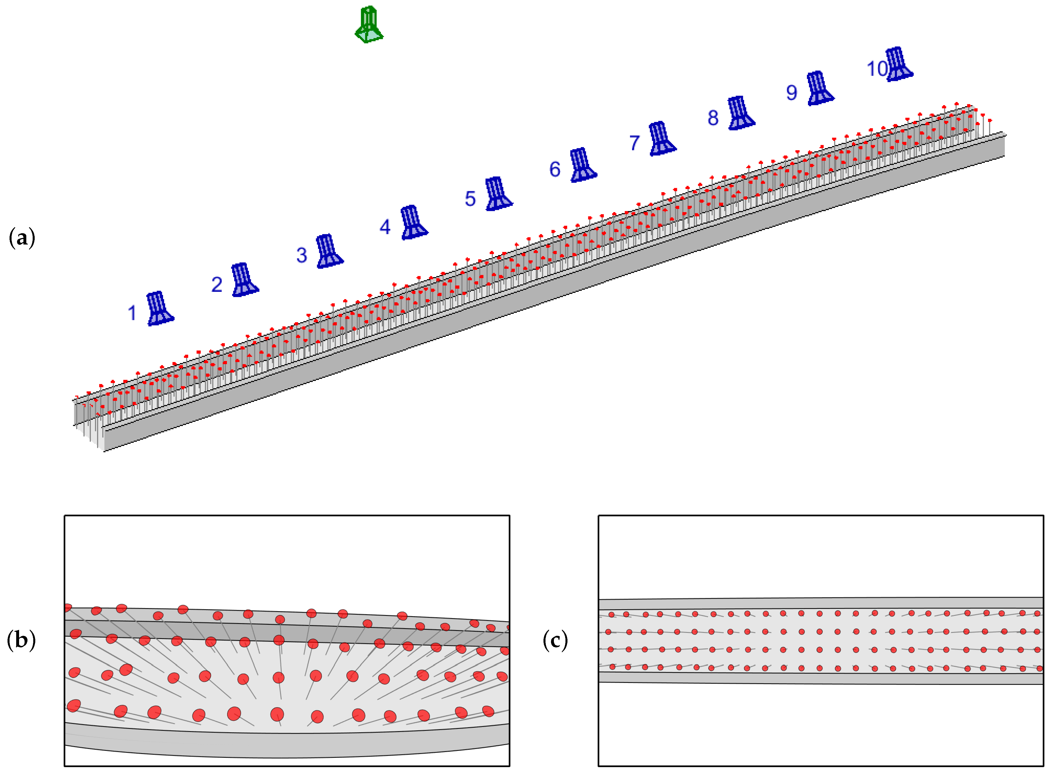
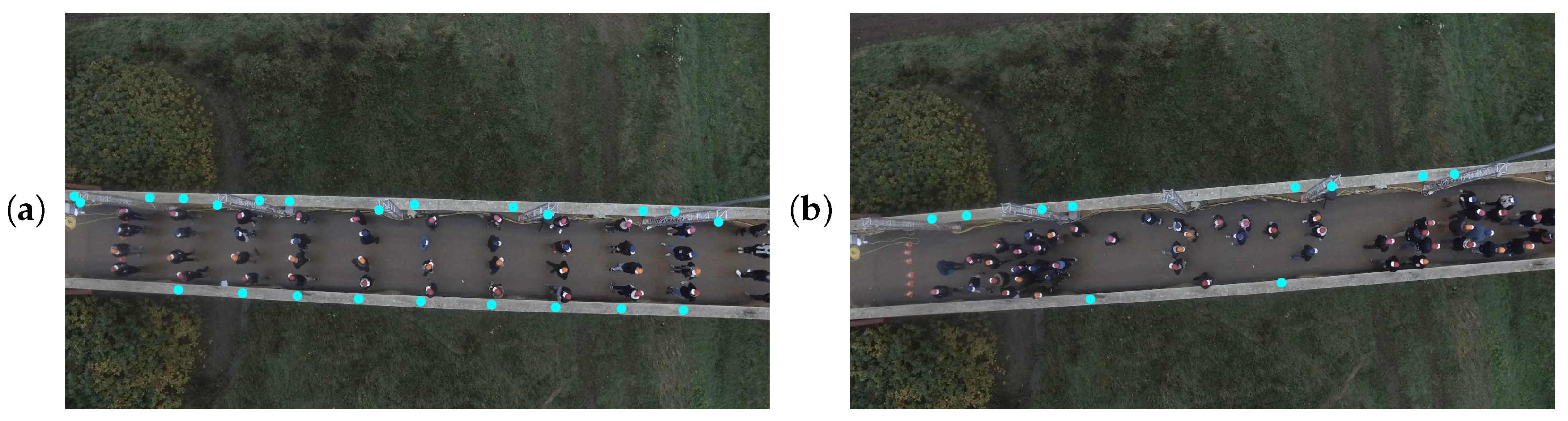
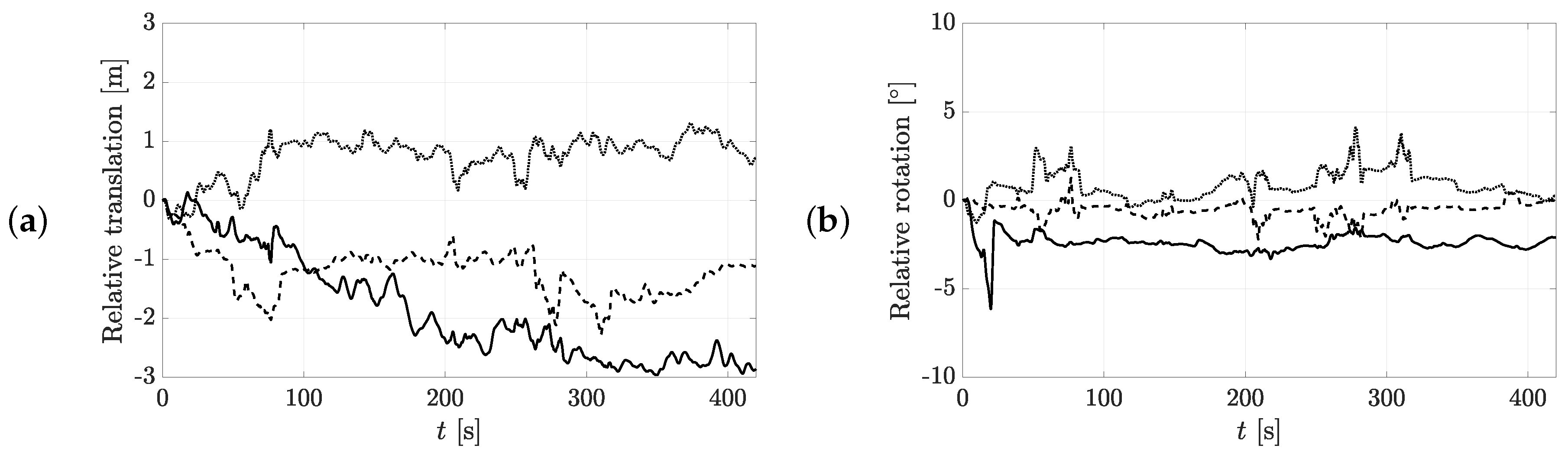
4.1.3. Position and Orientation Estimation of the Drone

In contrast to the static cameras, where no relative movement occurs because of the firm fixation to the aluminum trusses, the drone is subjected to non-negligible changes in position and orientation due to wind loading. This poses a problem since the calibration is only performed on the initial frame. It is observed that the intrinsic camera parameters, $\mathbf{K}$, and radial distortion coefficients, $[{\kappa }_1,{\kappa }_2,{\kappa }_3]$, do not change, and therefore it is only needed to compute the position $\mathbf{t}$ and orientation ${\Theta }$ of the drone of each frame. The calibration points (×-shaped marks on the bridge deck) are tracked among the different frames using the Kanade–Lucas–Tomasi (KLT) tracking algorithm [53,54] (function PointTracker). The latter is particularly suited for tracking objects that do not change shape and possess a visual texture. The tracker is configured using 3 image pyramid levels, a rectangular neighborhood block size of 51 pixels and a maximum forward-backward error threshold of 10 pixels. A reliability score for each tracker point is computed accounting for the singularity of the spatial gradient and verifies if the maximum reprojection error does not exceed the user-defined value. Tracked points with a reliability less than 0.95 are excluded from further analysis. The retained tracked points are used to estimate the pose using the 3D-2D correspondences using the same procedure as in Section 4.1.2 but with the internal parameters $[{\alpha }_x$, ${\alpha }_y$, $u_x$, $u_y]$ and radial distortion coefficients $[{\kappa }_1$,${\kappa }_2$,${\kappa }_3]$ already known.

An example of the pose estimation algorithm is shown in Figure 15, where the calibration points on the initial frame (Figure 15a) are tracked on the 600th frame (Figure 15b). One can notice that not all calibration points are found on the 600th frame, as only the points are retained of which the reliability score is sufficiently high. The relative movements (Figure 16) show that the change in pose is primarily dominated by translational changes and, to a lesser degree, some rotational changes.

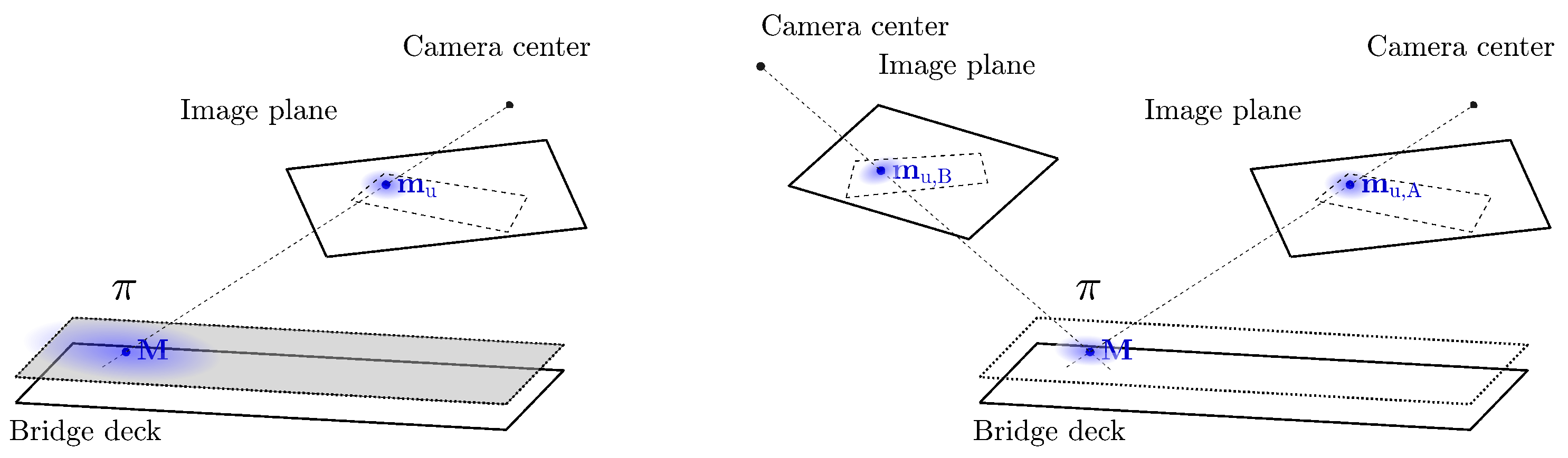
4.1.4. Retrieving the 3D Position Using Stereo-View Geometry: Triangulation

If a point (or hat) is visible in two (or more) cameras A and B with camera projection matrices ${\mathbf{P}}_{\mathrm{A}}$ and ${\mathbf{P}}_{\mathrm{B}}$ and with the undistorted image coordinates ${\mathbf{m}}_{\mathrm{u},\mathrm{A}}$ and ${\mathbf{m}}_{\mathrm{u},\mathrm{B}}$, its 3D location can be obtained using triangulation (Figure 17a). The 3D location is found for the point $\mathbf{M}$ for which the following holds:

$$\begin{array}{c}\hfill \left\{\begin{array}{cc}{\mathbf{m}}_{\mathrm{u},\mathrm{A}}& ={\mathbf{P}}_{\mathrm{A}}\mathbf{M}\\ {\mathbf{m}}_{\mathrm{u},\mathrm{B}}& ={\mathbf{P}}_{\mathrm{B}}\mathbf{M}\end{array}\right.\end{array}$$

(6)

Due to the presence of measurement errors, no exact solution exists. In [51] an iterative procedure is proposed which obtains $\mathbf{M}$ by minimizing the reprojection error.

4.1.5. Retrieving the 3D Position Using Mono-View Geometry: Homography

In general, one needs stereo vision to retrieve the 3D location of an object. If, however, additional information is available it might be possible to retrieve the world coordinates based on a single 2D image. In our case, the height of every pedestrian is known. One can therefore define a plane $\pi$, parallel to the bridge deck with a distance equal to the participant’s height. The detection should lie on this plane and thus a planar homography can be used to relate a measured image coordinate to a corresponding world location (Figure 17b). Hartley and Zisserman developed a methodology to obtain a homography between the image plane and plane $\pi$ if 4 correspondence points on the plane are known [52]. While easy to use since the projection matrix $\mathbf{P}$ of the camera is not required, an important drawback is that for every pedestrian (which has his own height) 4 calibration points are needed. Theoretically this would require 148 × 4 points per camera. To overcome this cumbersome procedure, the homography is instead directly calculated using the projection matrix $\mathbf{P}$ of the camera and the pedestrian’s height, as described in Appendix A. The latter procedure is possible since the projection matrix $\mathbf{P}$ of each camera is known in the present study.

The relation between the undistorted homogeneous image and world point is described by a planar homography in case of mono-vision geometry:

$${\mathbf{m}}_{\mathrm{u}}=\left[\begin{array}{c}{x}_{\mathrm{u}}\\ y_{\mathrm{u}}\\ w_{\mathrm{u}}\end{array}\right]\simeq {\mathbf{H}}_{\pi }\left[\begin{array}{c}X\\ Y\\ W\end{array}\right].$$

(7)

When expressed in Euclidean coordinates the relation between the world location and detection on the image plane becomes non-linear:

$$\left[\begin{array}{c}{x}_{\mathrm{u}}/w_{\mathrm{u}}\\ y_{\mathrm{u}}/w_{\mathrm{u}}\end{array}\right]=\left[\begin{array}{c}\frac{{\mathbf{H}}_{{\pi }_1}{[X,Y,1]}^{\mathrm{T}}}{{\mathbf{H}}_{{\pi }_3}{[X,Y,1]}^{\mathrm{T}}}\\ \frac{{\mathbf{H}}_{{\pi }_2}{[X,Y,1]}^{\mathrm{T}}}{{\mathbf{H}}_{{\pi }_3}{[X,Y,1]}^{\mathrm{T}}}\end{array}\right]$$

(8)

with ${\mathbf{H}}_{\pi ,j}$ the jth row of the homography ${\mathbf{H}}_{\pi }$.

4.2. Trajectory Reconstruction Using a Kalman Filter

Multiple pedestrians and the occasional occurrence of misdetections (precision ≤ 100%, Section 3) result in a multi-object data association problem. In addition, the measurements are subject to measurement errors. To ensure a reliable and robust data association, a Kalman filter (KF) [55] is used as a motion-based estimator of a pedestrian’s position in consecutive frames.

The KF is configured with a state-space matrix using the constant-velocity assumption. This choice is motivated given the higher frame rate of the cameras (30 fps, Section 2.1). The frame rate is high relative to the expected walking speed (≈5 km/h) and the body movement (average step frequency 1.8 Hz = 0.56 $\frac{1}{\mathrm{s}}$).

Given the employed state-space model, the state vector contains the position and velocity of the pedestrian. In case the observations are made in stereo view, the X, Y and Z coordinate are considered. In the mono-view case, the vertical Z coordinate is dropped as it is predefined by the plane $\pi$ (Section 4.1.5).

To establish the measurement vector of a pedestrian, its a priori estimate of the location is projected onto the image plane(s) of the closest camera(s) (Equation (5)). The detection whose distance is minimal. A maximal distance threshold of 20 pixels (≈120 mm ground distance ≈1 radius of a pedestrian’s hat, Section 2.1) is defined. If no detections are found within this distance, there is no measurement for that time step.

The observation matrix relates the measurement and state vector. Both vectors are expressed in world coordinates. Although the velocity is not directly measured, it is obtained as a result of the Kalman filter process by applying the state transition matrix.

Random errors are present in the measurements. A partial detection and the application of morphological operations (Figure 10) on the raw detection mask result in a deviation of the detected centroid with respect to the true one. The random measurement error in the image plane is modeled using a bivariate normal distribution with no correlation between the horizontal and vertical direction and between different frames. The variance in both directions is assumed identical in the image plane. Hence, the covariance matrix describing the measurement error in the image plane is a diagonal matrix and the 95% confidence region of the detections in the image plane are described by circles. It is observed that for the static cameras the blob sizes are bigger in the center compared to the ones at the sides of the image. For the drone, the blob size is nearly constant over the entire image width. Therefore, the variance in case of the static camera setup is assigned a value of 12² pixels² in the middle of the image, linearly decreasing to a value of 5² pixels² at the vertical sides of the image plane. For the drone, a constant value of 5² pixels² is adopted. The values are chosen empirically as it is observed that their corresponding 95% confidence regions include the hat of the pedestrians for all possible locations on the image (Figure 18).

The probability density function (PDF) of the random measurement noise of the detection is defined in the image plane. The measurements are, on the other hand, expressed in the world space coordinates. A conversion of the PDF defined on the image plane(s) to the corresponding world space is required. In case of mono conversion, change of stochastic variables is employed to obtain the PDF of the measurement in world coordinates [56]. For the stereo case, the mapping is no longer one-to-one and therefore the PDF is calculated numerically. Each location on the bridge deck is projected onto the two corresponding images. Next, a grid on both images is defined covering the 95% confidence domain. Every possible combination of the gridpoints on both planes is considered, its corresponding 3D world location is calculated (Section 4.1.4) and the corresponding probability is assigned to that point. Finally, a trivariate normal distribution is fitted on the obtained point cloud where each point has a certain probability which allows the obtaining of the covariance matrix of the measurement of the stereo case in world coordinates. The 95% confidence intervals indicate that the measurement noise in world coordinates is no longer uncorrelated among the different directions (Figure 19). To compare both error covariance matrices, the stereo error is projected onto the horizontal plane. In addition, the major axis of the 95% of the (horizontally projected) uncertainty ellipse is calculated (Figure 20). In the case of the mono-vision setup, the maximum horizontal random measurement error varies between 15 cm and 25 cm and increases with the distance from the camera. For the stereo vision setup, the maximum horizontal random measurement error is in the order of magnitude of 10 cm and is nearly constant over the bridge deck. The comparison illustrates that the uncertainty related to the random measurement error is larger in case of mono-vision. Figure 21 and Figure 22 show the confidence regions and corresponding maximal horizontal random measurement error of the mono conversion for the drone. The maximum horizontal random measurement error is nearly constant over the bridge deck (within the FOV) and in the same order of magnitude as for the mono-vision setup of the static cameras This is a logical consequence of the fact that the 95% confidence region was defined to capture a pedestrian’s hat in the image plane for both camera setups.

Besides the random measurement errors, ystematic errors (i.e., errors which are correlated over consecutive time steps) are also present by the fact that the pedestrian’s hat (represented by a hemisphere) is not projection invariant. Therefore, the center of mass of the head does not coincide with the centroid of the projected hemisphere (Figure 23 left). In case of mono-view, an additional systematic error is induced by the vertical sway of the head as a result of the walking locomotion. As such, the homography which assumes that the center of mass lies on the plane defined by the homography (Section 4.1.5) is an approximation of the real situation (Figure 23 right). Because the aforementioned sources of error are systematic instead of random, they are not removed by the Kalman filter and smoother. Their influence on the result is investigated in Section 5.1. A third cause of systematic measurement error are the imperfect calibration of the cameras. However, given the low reprojection error obtained after calibration (Section 4.1.2) it is assumed that this source of systematic error is negligible compared to the other ones.

It is not straightforward to define the process noise matrix. To avoid an arbitrarily assignment of its value, the expectation maximum algorithm [57] is employed. The method uses the entire set of smoothed observations and measurements. The optimal process noise matrix is found for which the likelihood of occurrence of the measurement vector is maximized. A closed-form expression is provided in [57].

The process is executed using an initial estimate of the process noise covariance with a variance of (0.10 m)² and (0.05 m/s)² for the locations and velocities and zero covariance among the variables is. The online KF and RTS smoother yield the smoothed results. Then, an optimal process noise matrix is estimated. The process is repeated until convergence is attained.

5. Results and Discussion

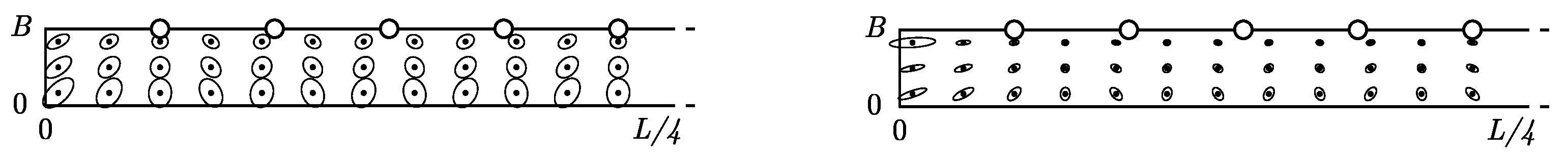
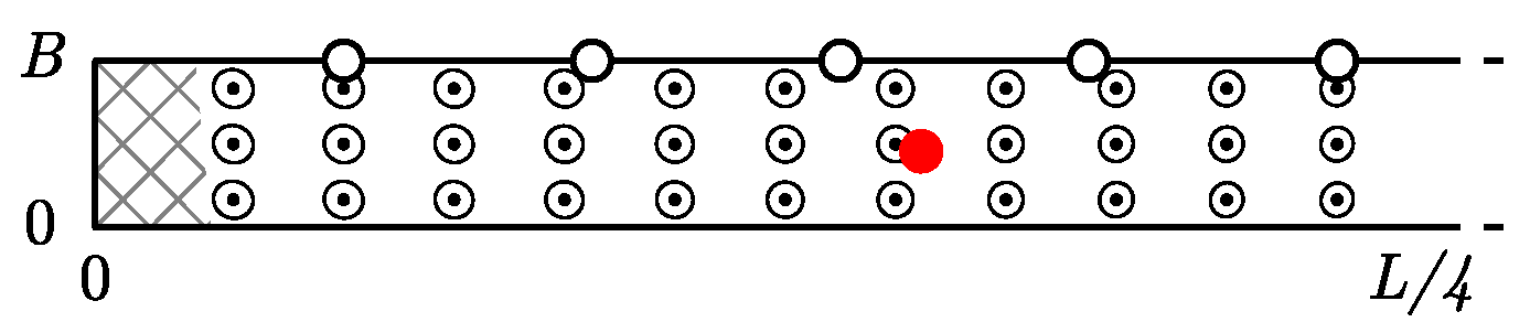
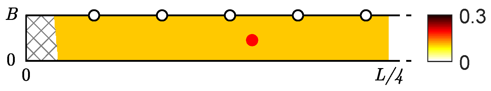
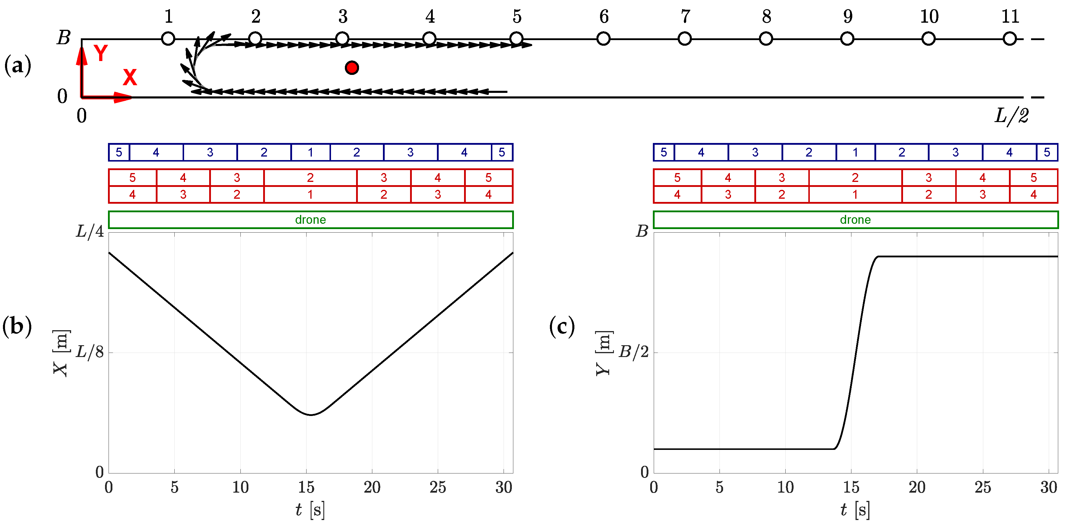
5.1. Theoretical Example to Evaluate the Effect of the Systematic Measurement Errors

Besides the random measurement noise, systematic errors in the obtained trajectories are present (Figure 23). To evaluate their effect, a theoretical example is first considered. A camera setup identical to the one of the large-scale measurement campaign is used (Section 2.1). The theoretical trajectory consists of a walking pedestrian along a quarter bridge deck and turning around at static camera 1 with a lateral position of 0.4 m and 2.6 m (Figure 24a). The Z-coordinate of the pedestrian’s head is assumed to be 1.7 m above the bridge deck. Along its trajectory, the pedestrian is visible in multiple cameras depending on the considered setup (mono or stereo vision, Figure 24b,c). As this is a purely theoretical situation, no random measurement error is present and hence the only discrepancy between true and estimated trajectory stems from the modeled systematic errors: the projection-variant shape of the shape of the hat (Section 5.1.1) and the vertical sway of the pedestrian’s head during the walking (Section 5.1.2).

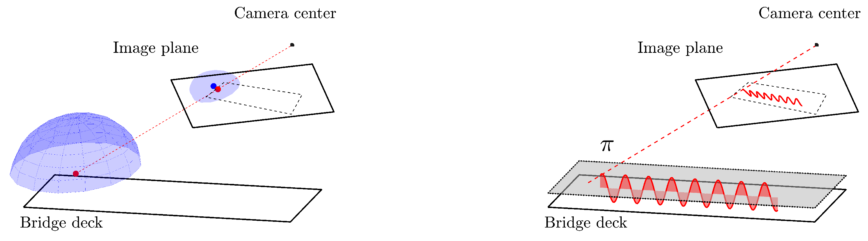
5.1.1. Effect of the Shape of the Hat

The effect of the shape is investigated by modeling the colored hat as hemisphere with radius $r=0.10$ m (Section 2.1). The centroid of the deformed projection is obtained using a blob analyzer (Section 3) while the corresponding (world) trajectory is determined employing the presented either triangulation (stereo vision, Section 4.1.4) or a homography (mono-vision, Section 4.1.5). The difference between the true trajectory and the measured trajectory (including the systematic error) is calculated. In addition the difference between the trajectories obtained by the static and drone camera is determined. The results (Figure 25) show that the maximum induced error is 4 cm for all measurement setups and depends on the location of the pedestrian and increases with the obliqueness of the viewing angle (Figure 25a–c). The maximum relative difference of between the trajectories obtained by the static and drone camera setup are respectively 6 cm in case of the mono-setup and 4 cm in case of the stereo vision setup (Figure 25d).

5.1.2. Effect of the Vertical Sway of the Head

The evaluate the vertical sway of the head, a vertical sinusoidal movement with an amplitude of 2 cm and a frequency of 2 Hz is superimposed on the vertical Z-coordinate of the trajectory. To exclude of the influence of the shape of the hat, it is now modeled with a point instead of a hemisphere. The point is projected onto the image planes (Equation (5)) and its (horizontal) world position is calculated. The results (Figure 26a–c) show that the maximum error between the true trajectory and the trajectory identified by the camera system is 2 cm for the measurement setups involving a single camera and no error is introduced in case of the stereo vision setup. Indeed, the vertical sway of the head does not introduce a horizontal error in case of stereo vision since no prior assumption is made with respect to a predefined plane on which the detection should lie (Section 4.1.5). When the results of the static setup are compared to the trajectories of obtained by the drone setup (Figure 26d), an absolute difference in the order of magnitude of 2 cm is observed.

5.2. Experimental Results

5.2.1. Obtained Trajectories

Figure 27a,b show a heat map of the trajectory for the case of walking (test 9, 0.50 $\mathrm{pers}./{\mathrm{m}}^2$, Table 1) of a single participant and the whole group, respectively. In Figure 27b a certain degree of lane formation can be noticed. Although the authors recognize that the considered test setup is artificial, lane formation in the flow of a high-density crowd is a phenomenon that has been predicted by numerical calculations using theoretical social force models describing pedestrian dynamics [20].

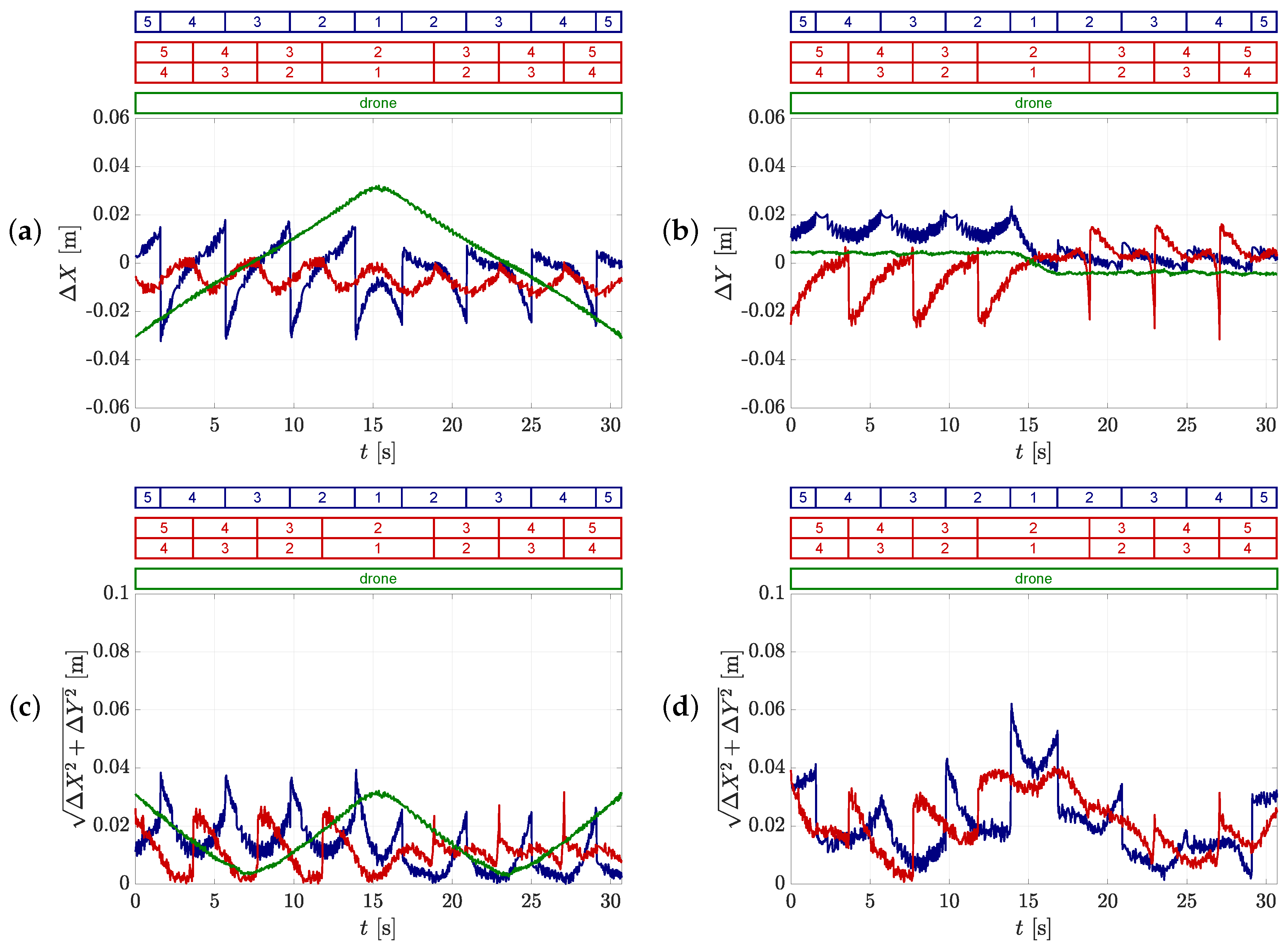
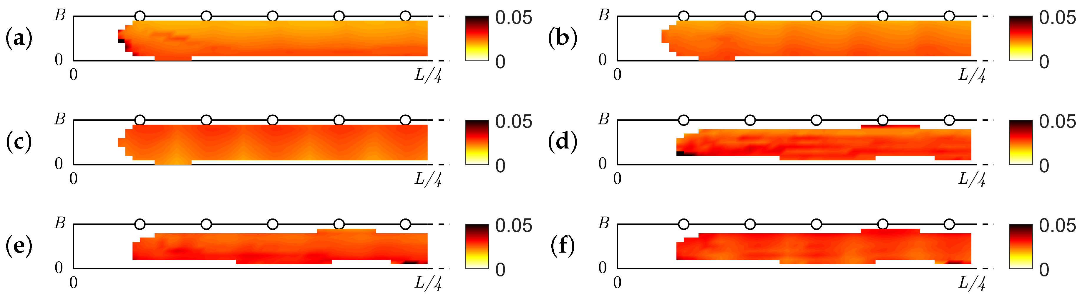
5.2.2. Uncertainty of the Obtained Trajectories by the Static Camera Setup

Figure 28 depicts the maximum horizontal uncertainty of the estimated state (location) for both the case of walking and jogging. The uncertainty is calculated as the major axis of the 95% confidence ellipse, related to the covariance of the smoothed state, ${{\Sigma }}_{k|N}$. This Figure shows that after application of the Kalman smoothing a similar horizontal uncertainty is found for both measurement methods (stereo and mono) and is nearly constant over the bridge deck, as opposed to the maximum random measurement error. Furthermore, it is noticed that the uncertainty is somewhat higher for jogging (order of magnitude of 3–4 cm) than walking (order of magnitude 2–3 cm) as a result of the higher speed. The frame rate is the same, but the jogging speed is higher resulting in a larger movement between frames. The prescribed constant motion model slightly deviates from the true trajectory, resulting in a larger measurement residual and thus higher uncertainty of the optimal estimated state.

Figure 29 shows an example of the application of the pedestrian trajectory reconstruction procedure (Section 4.2) where it is clearly illustrated that the initial state uncertainty, as obtained by the measurement, is drastically reduced after applying the Kalman filtering and smoothing.

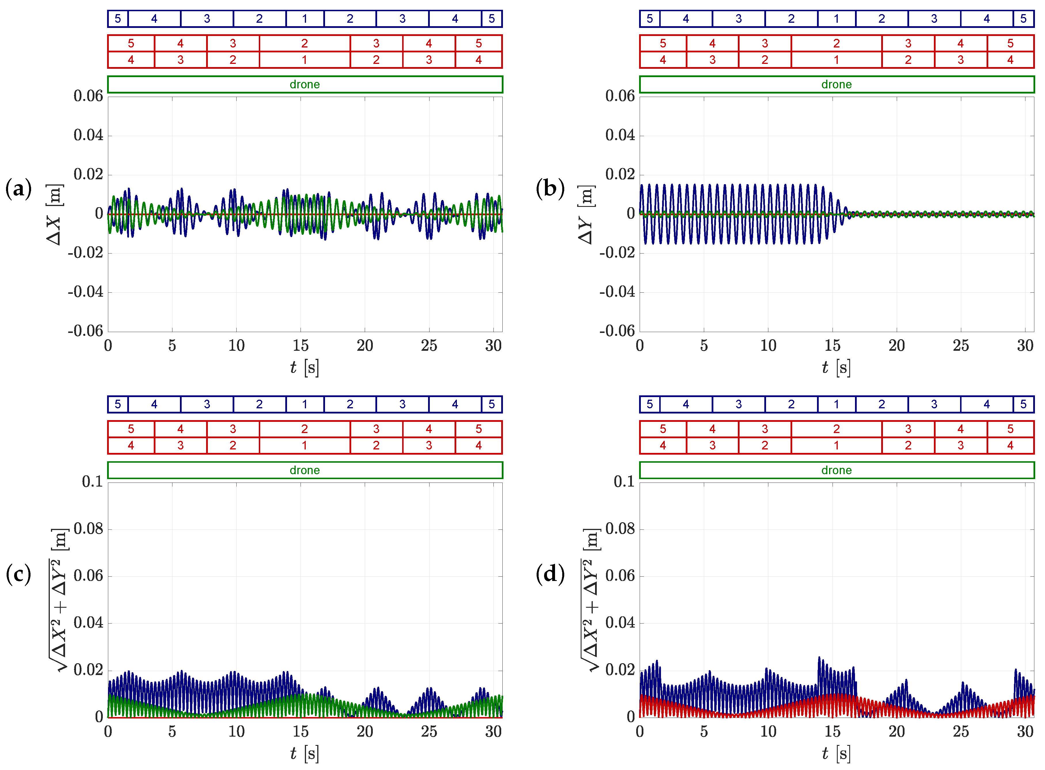
5.2.3. Uncertainty of the Obtained Trajectories with the Drone

The maximum horizontal uncertainty of the trajectories obtained with the drone is in the order of magnitude of 2 cm, nearly constant over the bridge deck and similar for mono and EKF conversion (Figure 30). This uncertainty is also in the same order of magnitude as obtained for the static camera setup (Section 5.2.2).

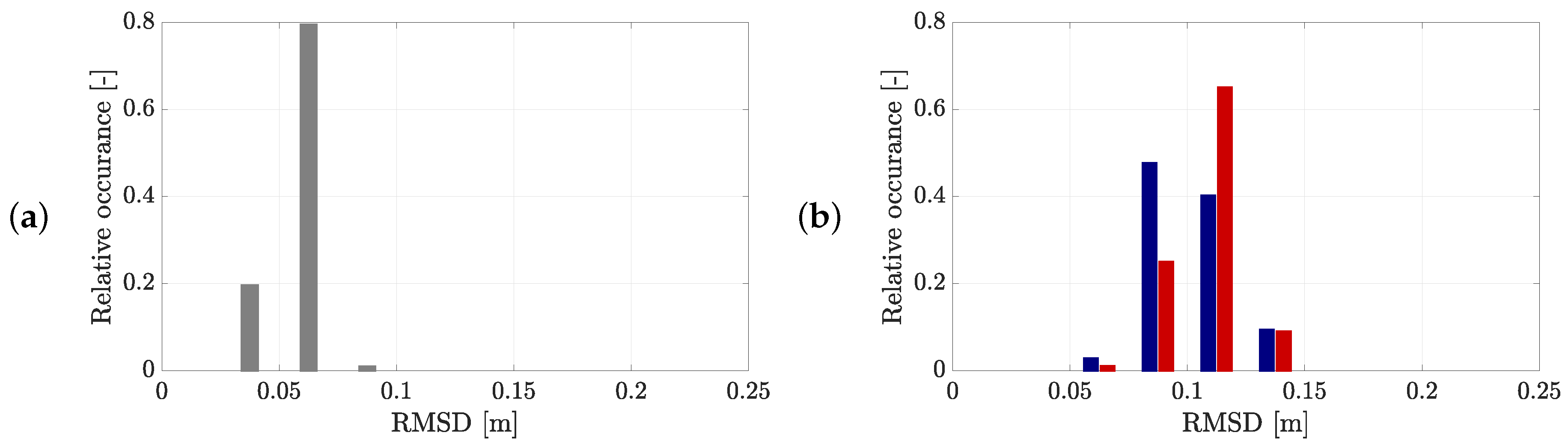
5.2.4. Comparison of the Different Camera Setups

The trajectories obtained by the different camera setups (static versus drone and static stereo versus static mono-vision) are compared by calculating the Root Mean Squared Differences (RMSD) (Figure 31), which is a combination of the average random and systematic error. The comparison of the static mono and static stereo setup (Figure 31a) reveals that the majority of the tracks deviate less than 7.5 cm. Comparing the obtained trajectories of the static setup with the drone setup (Figure 31b) shows that the difference is less than 15 cm for all the obtained trajectories, for both the mono and stereo setup. The difference for the stereo setup is somewhat higher than for the mono setup. Since the comparison is a combination of both the systematic and random errors, the differences are higher than those given by the uncertainty of the smoothed state (Section 5.2.2 and Section 5.2.3).

6. Conclusions

The ambition of this study is to develop a measurement setup allowing accurate and robust obtaining of the trajectories of a high-density crowd on footbridges. A case study of a large-scale measurement campaign is presented, involving pedestrian densities up to 0.50 pers/m² and considering both walking and jogging events. The setup consisted of 21 static cameras with sufficient overlap to allow mono and stereo vision. The related measurement accuracy of both methods is assessed and revealed that the accuracy of the stereo vision is higher compared to the mono-view setup. To minimize the effect of the random measurement error a Kalman filter and smoother are implemented. As a result, the uncertainty of the final trajectories is reduced to a fraction of the measurement uncertainty, yielding similar results for both conversions in case of walking (2–3 cm) and jogging (4–5 cm). Also, the systematic error introduced by the shape of the hat and the walking locomotion of the participants is investigated and is observed to be less than 6 cm. Besides the static camera setup, a drone was used to additionally record a part of the bridge deck during operation. Similar observations with respect to the uncertainty as the static camera setup are found. The different measurement methods (mono/stereo static setup and mono-drone setup) are compared by calculating the Root Mean Squared Differences (RMSD). This quantity comprises both systematic and random errors and is found to be less than 15 cm for all collected trajectories. Therefore, it is concluded that the envisaged accuracy for structural dynamics purposes (15 cm) is largely attained.

Although the methodology is applied on a specific case study, the camera setup, measurement methodology and post-processing strategy are generic since an extension to a bridge with virtually any length is possible. The collected empirical trajectories allow a calibration of the parameters of the pedestrian dynamics model for the specific situation of crowd flows on footbridges. Moreover, together with the other collected quantities (3D body motion and structural accelerations), a benchmark data set is obtained which should find use in the further development and calibration of load models that describe human-induced loading on footbridges.

References

1. Brunetti, A.; Buongiorno, D.; Trotta, G.F.; Bevilacqua, V. Computer vision and deep learning techniques for pedestrian detection and tracking: A survey. Neurocomputing 2018, 300, 17–33. [Google Scholar] [CrossRef]
2. Cao, Y.; Guan, D.; Huang, W.; Yang, J.; Cao, Y.; Qiao, Y. Pedestrian detection with unsupervised multispectral feature learning using deep neural networks. Inf. Fusion 2019, 46, 206–217. [Google Scholar] [CrossRef]
3. Khalifa, A.F.; Badr, E.; Elmahdy, H.N. A survey on human detection surveillance systems for Raspberry Pi. Image Vis. Comput. 2019, 85, 1–13. [Google Scholar] [CrossRef]
4. Hou, Y.L.; Song, Y.; Hao, X.; Shen, Y.; Qian, M.; Chen, H. Multispectral pedestrian detection based on deep convolutional neural networks. Infrared Phys. Technol. 2018, 94, 69–77. [Google Scholar] [CrossRef]
5. Chen, Y.; Zhao, D.; Lv, L.; Zhang, Q. Multi-task learning for dangerous object detection in autonomous driving. Inf. Sci. 2018, 432, 559–571. [Google Scholar] [CrossRef]
6. Campmany, V.; Silva, S.; Espinosa, A.; Moure, J.; Vázquez, D.; López, A. GPU-based pedestrian detection for autonomous driving. Procedia Comput. Sci. 2016, 80, 2377–2381. [Google Scholar] [CrossRef] [Green Version]
7. Bruno, L.; Corbetta, A. Uncertainties in crowd dynamic loading of footbridges: A novel multi-scale model of pedestrian traffic. Eng. Struct. 2017, 147, 545–566. [Google Scholar] [CrossRef]
8. Ahmadi, E.; Caprani, C.; Heidarpour, A. An equivalent moving force model for consideration of human-structure interaction. Appl. Math. Model. 2017, 51, 526–545. [Google Scholar] [CrossRef]
9. Ahmadi, E.; Caprani, C.; Živanović, S.; Heidarpour, A. Vertical ground reaction forces on rigid and vibrating surfaces for vibration serviceability assessment of structures. Eng. Struct. 2018, 172, 723–738. [Google Scholar] [CrossRef]
10. Georgakis, C.T.; Ingólfsson, E. Recent advances in our understanding of vertical and lateral footbridge vibrations. In Proceedings of the 5th International Footbridge Conference, Crete, Greece, 22–27 June 2014. [Google Scholar]
11. Živanović, S. Benchmark Footbridge for Vibration Serviceability Assessment under Vertical Component of Pedestrian Load. J. Struct. Eng. 2012, 138, 1193–1202. [Google Scholar] [CrossRef] [Green Version]
12. Wei, X.; Van den Broeck, P.; De Roeck, G.; Van Nimmen, K. A simplified method to account for the effect of human-human interaction on the pedestrian-induced vibrations of footbridges. In Proceedings of the 10th International Conference on Structural Dynamics, EURODYN 2017, Rome, Italy, 10–13 September 2017. [Google Scholar]
13. Van Hauwermeiren, J.; Van Nimmen, K.; Van den Broeck, P. The effect of the spatial distribution of crowds on the structural response to pedestrian excitation. In Proceedings of the 13th International Conference on Recent Advances in Structural Dynamics, Lyon, France, 15–17 April 2019. [Google Scholar]
14. Helbing, D.; Molnar, P. Social force model for pedestrian dynamics. Phys. Rev. 1995, 51, 4282–4286. [Google Scholar] [CrossRef] [PubMed] [Green Version]
15. Haghani, M.; Sarvi, M.; Shahhoseini, Z.; Boltes, M. Dynamics of social groups’ decision-making in evacuations. Transp. Res. Part C Emerg. Technol. 2019, 104, 135–157. [Google Scholar] [CrossRef]
16. Von Krüchten, C.; Schadschneider, A. Empirical study on social groups in pedestrian evacuation dynamics. Phys. A Stat. Mech. Its Appl. 2017, 475, 129–141. [Google Scholar] [CrossRef] [Green Version]
17. Karamouzas, I.; Heil, P.; van Beek, P.; Overmars, M.H. A Predictive Collision Avoidance Model for Pedestrian Simulation. In Motion in Games; Egges, A., Geraerts, R., Overmars, M., Eds.; Springer: Berlin/Heidelberg, Germany, 2009; pp. 41–52. [Google Scholar]
18. Van den Berg, J.; Guy, S.; Lin, M.; Manocha, D. Reciprocal n-Body Collision Avoidance. Springer Tracts Adv. Robot. 2011, 70, 3–19. [Google Scholar] [CrossRef]
19. Reynolds, C.W. Flocks, Herds and Schools: A Distributed Behavioral Model. In SIGGRAPH Computer Graphics; Association for Computing Machinery: New York, NY, USA, 1987; pp. 25–34. [Google Scholar]
20. Helbing, D.; Buzna, L.; Johansson, A.; Werner, T. Self-Organized Pedestrian Crowd Dynamics: Experiments, Simulations, and Design Solutions. Transp. Sci. 2005, 39, 1–24. [Google Scholar] [CrossRef] [Green Version]
21. Fujino, Y.; Pacheco, B.; Nakamura, S.I.; Warnitchai, P. Synchronization of human walking observed during lateral vibration of a congested pedestrian bridge. Earthq. Eng. Struct. Dyn. 1993, 22, 741–758. [Google Scholar] [CrossRef]
22. Dallard, P.; Fitzpatrick, A.J.; Flint, A.; Le Bourva, S.; Low, A.; Ridsdill Smith, R.M.; Willford, M. The London Millennium Footbridge. Struct. Eng. 2001, 79, 17–33. [Google Scholar]
23. Setareh, M. Study of Verrazano-Narrows Bridge Movements during a New York City Marathon. J. Bridge Eng. 2011, 16, 127–138. [Google Scholar] [CrossRef]
24. Macdonald, J.H.G. Pedestrian-induced vibrations of the Clifton Suspension Bridge, UK. Proc. Inst. Civ. Eng. Bridge Eng. 2008, 161, 69–77. [Google Scholar] [CrossRef]
25. Dang, H.V.; SŽivanović, S. Experimental characterisation of walking locomotion on rigid level surfaces using motion capture system. Eng. Struct. 2015, 91, 141–154. [Google Scholar] [CrossRef] [Green Version]
26. McDonald, M.G.; Živanović, S. Measuring Ground Reaction Force and Quantifying Variability in Jumping and Bobbing Actions. J. Struct. Eng. 2017, 143. [Google Scholar] [CrossRef]
27. Dang, H.V.; Živanović, S. Influence of Low-Frequency Vertical Vibration on Walking Locomotion. J. Struct. Eng. 2016, 142. [Google Scholar] [CrossRef]
28. Racic, V.; Brownjohn, J.; Pavic, A. Reproduction and application of human bouncing and jumping forces from visual marker data. J. Sound Vib. 2010, 329, 3397–3416. [Google Scholar] [CrossRef]
29. Carroll, S.; Owen, J.; Hussein, M. Reproduction of lateral ground reaction forces from visual marker data and analysis of balance response while walking on a laterally oscillating deck. Eng. Struct. 2013, 49, 1034–1047. [Google Scholar] [CrossRef]
30. Bocian, M.; Brownjohn, J.; Racic, V.; Hester, D.; Quattrone, A.; Monnickendam, R. A framework for experimental determination of localised vertical pedestrian forces on full-scale structures using wireless attitude and heading reference systems. J. Sound Vib. 2016, 376, 217–243. [Google Scholar] [CrossRef] [Green Version]
31. Neges, M.; Koch, C.; König, M.; Abramovici, M. Combining visual natural markers and IMU for improved AR based indoor navigation. Adv. Eng. Inform. 2017, 31, 18–31. [Google Scholar] [CrossRef]
32. Kang, W.; Han, Y. SmartPDR: Smartphone-based pedestrian dead reckoning for indoor localization. IEEE Sens. J. 2015, 15, 2906–2916. [Google Scholar] [CrossRef]
33. Tian, Q.; Salcic, Z.; Wang, K.I.; Pan, Y. A Multi-Mode Dead Reckoning System for Pedestrian Tracking Using Smartphones. IEEE Sens. J. 2016, 16, 2079–2093. [Google Scholar] [CrossRef]
34. Poulose, A.; Han, D.S. Hybrid indoor localization using IMU sensors and smartphone camera. Sensors 2019, 19, 5084. [Google Scholar] [CrossRef] [Green Version]
35. Xing, B.; Zhu, Q.; Pan, F.; Feng, X. Marker-based multi-sensor fusion indoor localization system for micro air vehicles. Sensors 2018, 18, 1706. [Google Scholar] [CrossRef] [Green Version]
36. Mirshekari, M.; Pan, S.; Fagert, J.; Schooler, E.M.; Zhang, P.; Noh, H.Y. Occupant localization using footstep-induced structural vibration. Mech. Syst. Signal Process. 2018, 112, 77–97. [Google Scholar] [CrossRef]
37. Boltes, M.; Seyfried, A. Collecting pedestrian trajectories. Neurocomputing 2013, 100, 127–133. [Google Scholar] [CrossRef]
38. Haghani, M.; Sarvi, M. Herding in direction choice-making during collective escape of crowds: How likely is it and what moderates it? Saf. Sci. 2019, 115, 362–375. [Google Scholar] [CrossRef]
39. Shahhoseini, Z.; Sarvi, M. Pedestrian crowd flows in shared spaces: Investigating the impact of geometry based on micro and macro scale measures. Transp. Res. Part B Methodol. 2019, 122, 57–87. [Google Scholar] [CrossRef]
40. Feliciani, C.; Nishinari, K. Measurement of congestion and intrinsic risk in pedestrian crowds. Transp. Res. Part C Emerg. Technol. 2018, 91, 124–155. [Google Scholar] [CrossRef]
41. Shi, X.; Ye, Z.; Shiwakoti, N.; Tang, D.; Lin, J. Examining effect of architectural adjustment on pedestrian crowd flow at bottleneck. Phys. A Stat. Mech. Its Appl. 2019, 522, 350–364. [Google Scholar] [CrossRef] [Green Version]
42. Van Hauwermeiren, J.; Van den Broeck, P.; Van Nimmen, K.; Vergauwen, M. Vision-based methodology for characterizing the flow of a high-density crowd. In Proceedings of the 9th International Conference on Bridge Maintenance, Safety and Management, Melbourne, Australia, 9–13 July 2018; Taylor and Francis Group, CRC Press: Melbourne, Australia, 2018. [Google Scholar]
43. Van Nimmen, K.; Lombaert, G.; Jonkers, I.; De Roeck, G.; Van den Broeck, P. Characterisation of walking loads by 3D inertial motion tracking. J. Sound Vib. 2014, 333, 5212–5226. [Google Scholar] [CrossRef] [Green Version]
44. Triggs, B.; McLauchlan, P.F.; Hartley, R.I.; Fitzgibbon, A.W. Bundle Adjustment: A Modern Synthesis. In Proceedings of the ICCV 99 Proceedings of the International Workshop on Vision Algorithms: Theory and Practice, Corfu, Greece, 21–22 September 1999. [Google Scholar]
45. Berns, R.; Billmeyer, F.; Saltzman, M. Billmeyer and Saltzman’s Principles of Color Technology; Wiley-Interscience, Wiley: Hoboken, NJ, USA, 2000; ISBN 9780471194590. [Google Scholar]
46. MATLAB Version 9.1.0.441655 (R2016b); The Mathworks, Inc.: Natick, MA, USA, 2017.
47. Thomas, S.W. Efficient inverse color map computation. Graph. Gems II 1991, 116–125. [Google Scholar] [CrossRef]
48. Lloyd, S.P. Least Squares Quantization in PCM. IEEE Trans. Inf. Theory 1982, 28, 129–137. [Google Scholar] [CrossRef]
49. Meyer, F. Topographic distance and watershed lines. Signal Process. 1994, 38, 113–125. [Google Scholar] [CrossRef]
50. Maurer, C.R., Jr.; Qi, R.; Raghavan, V. A Linear Time Algorithm for Computing Exact Euclidean Distance Transforms of Binary Images in Arbitrary Dimensions. IEEE Trans. Pattern Anal. Mach. Intell. 2003, 25, 265–270. [Google Scholar] [CrossRef]
51. Moons, T.; Gool, L.J.V.; Vergauwen, M. 3D Reconstruction from Multiple Images: Part 1—Principles. Found. Trends Comput. Graph. Vis. 2009, 4, 287–404. [Google Scholar] [CrossRef]
52. Hartley, R.; Zisserman, A. Multiple View Geometry in Computer Vision; Cambridge Books Online; Cambridge University Press: Cambridge, UK, 2003; ISBN 9780521540513. [Google Scholar]
53. Lucas, B.D.; Kanade, T. An Iterative Image Registration Technique with an Application to Stereo Vision. In Proceedings of the 7th International Joint Conference on Artificial Intelligence, Vancouver, BC, Canada, 24–28 August 1981. [Google Scholar]
54. Shi, J.; Tomasi, C. Good features to track. In Proceedings of the IEEE Conference on Computer Vision and Pattern Recognition, Seattle, WA, USA, 21–23 June 1994. [Google Scholar] [CrossRef]
55. Kalman, R.E. A New Approach to Linear Filtering And Prediction Problems. ASME J. Basic Eng. 1960, 82, 35–45. [Google Scholar] [CrossRef] [Green Version]
56. Bertsekas, D.; Tsitsiklis, J. Introduction to Probability; Athena Scientific Books; Athena Scientific: Nashua, NH, USA, 2002; ISBN 9781886529403. [Google Scholar]
57. Dempster, A.P.; Laird, N.M.; Rubin, D.B. Maximum likelihood from incomplete data via the EM algorithm. J. R. Stat. Soc. Ser. B 1977, 39, 1–38. [Google Scholar]
Figure 1. Impressions of the Eeklo footbridge during the large-scale measurement campaign: (a) top, (b) side and (c) below view.
Infrastructures 05 00051 g001
Figure 2. Plan view with indication of the position of the static cameras (blue dots), the highway (hatched areas) and orientation of the global axes (red arrows).
Infrastructures 05 00051 g002
Figure 3. Example of offline synchronization of the static camera setup based on the white van passing the white road marking: static camera 9 (left), 10 (middle) and 11 (right).
Infrastructures 05 00051 g003
Figure 4. Recording the pedestrians during the measurement campaign: (a) static camera setup and (b) pilot controlling drone during takeoff. The cameras are indicated with a red circle.
Infrastructures 05 00051 g004
Figure 5. Results of the preliminary study of the location and orientation of the static (blue) and drone (green) camera setup: (a) half a bridge deck with simulated grid of pedestrians with a red hat and a uniformly distributed random height between 1.6 m and 2.0 m. FOV of (b) static camera 3 and (c) the drone camera.
Infrastructures 05 00051 g005
Figure 6. Calibration points (width approximately 10 cm) on the bridge deck used to calibrate the cameras.
Infrastructures 05 00051 g006
Figure 7. Results of the preliminary study to select four hat colors: (a) snapshot of the candidate hats (b) one of the many snapshots of the background and (c) representation of the ( a * , b * ) coordinates of the colored hats (corresponding colors) and the background (black) by a heat map and 95% confidence regions (lines) and indication of the minimal distance between the 95% confidence regions of the selected hat colors to the background (dashed lines).
Infrastructures 05 00051 g007
Figure 8. Part of a snapshot reduced to a different amount of colors: (a) original frame, 2563 colors, (b) 1000 colors, and (c) 10 colors.
Infrastructures 05 00051 g008
Figure 9. k-means clustering procedure to distinguish detections from background shown in in the a*-b* plane of the CIELAB color space. The values of the pixels of the training frames (gray-shaded heat map), the a * and b * components of the (L)AB color map C AB (dots) indicating the values of the color map which correspond to a detection of a colored hat (corresponding colors) and background (black).
Infrastructures 05 00051 g009
Figure 10. Example of the color segmentation and detection algorithm: (a) original frame with indication of the true detected objects (white squares) and false detected objects (cyan squares), (b) binary mask before applying the morphological operations and (c) final binary image with indication of the detected color.
Infrastructures 05 00051 g010
Figure 11. Example of segmenting two adjacent detections (blue hats) employing the watershed transform: (a) original frame, (b) original binary mask, (c) binary distance with indication of watershed line and (d) binary mask after application of watershed segmentation.
Infrastructures 05 00051 g011
Figure 12. Flow chart for the detection of the pedestrians.
Infrastructures 05 00051 g012
Figure 13. Calibration of the static camera setup: (a) calibration frame of static camera 3 with indication of image correspondence points (△) and the reprojected world correspondence points (□) and (b) average reprojection error of the 21 calibrated static cameras.
Infrastructures 05 00051 g013
Figure 14. Calibration of the drone camera: (a) initial frame with indication of image correspondence points (△) and the reprojected world correspondence points (□) and (b) indication of the drone’s initial position relative to the bridge deck (red dot) and initial FOV (gray-shaded area).
Infrastructures 05 00051 g014
Figure 15. Example of the pose estimation algorithm using a KLT tracker: (a) initial frame with indication of calibration points (dots) and (b) 600th frame with retained calibration points using the KLT tracker.
Infrastructures 05 00051 g015
Figure 16. Relative movements of the drone to the original position and orientation as obtained from the position and orientation estimation algorithm: (a) translations along and (b) rotation around the X (dashed), Y (dotted) and Z (solid) axis.
Infrastructures 05 00051 g016
Figure 17. Conceptual illustration of the propagation of random measurement noise: an error in the image-plane results in an error in world coordinates for (left) mono and (right) stereo conversion. The PDF of the detections is represented by the shaded area on the image planes while the PDF of the obtained world coordinate is given by the shaded area on the plane π . In case of the stereo conversion, the PDF is projected onto the plane π as to only retain the horizontal uncertainty.
Infrastructures 05 00051 g017
Figure 18. Random measurement error of the detection in the image plane: (left) snapshot of the drone camera with the white dashed line indicating the (right) corresponding zoom with indication of the 95% confidence regions of the detections considering measurement noise (green lines) and the true detection of the pedestrians (green dots).
Infrastructures 05 00051 g018
Figure 19. Representation of the (horizontally projected) random measurement error covariance matrix of the static camera setup for a quarter of the bridge deck for (top) mono and (bottom) stereo vision: 95% confidence regions (lines) for different locations on the bridge deck (dots). The confidence regions are rescaled with a factor 3 around the true locations for illustration purposes.
Infrastructures 05 00051 g019
Figure 20. Maximum horizontal random measurement error of the static camera setup for (top) mono and (bottom) stereo setup for a quarter of the bridge deck. Colorbar expressed in meters.
Infrastructures 05 00051 g020
Figure 21. Representation of the random measurement error covariance matrix of the drone camera for a quarter of the bridge deck: 95% confidence regions (lines) for different locations on the bridge deck (dots). The confidence regions are rescaled with a factor 3 around the true locations for illustration purposes. The hatched area represents the part of the bridge deck that is outside the FOV of the camera.
Infrastructures 05 00051 g021
Figure 22. Maximum horizontal random measurement error of the drone camera. The red dot is the initial position of the drone. The hatched area represents the part of the bridge deck that is outside the FOV of the camera. Colorbar expressed in meters.
Infrastructures 05 00051 g022
Figure 23. Conceptual illustration of the systematically induced measurement errors: (left) the colored hat (blue hemisphere) is not projection invariant when projected onto the image plane (blue ellipsoid) and its centroid (blue dot) does not coincide with the projected center of mass of the sphere (red dot). (right) In case of mono-view, the vertical sway of the pedestrian’s head around the plane π induces an error as it does not coincide with the plane π .
Infrastructures 05 00051 g023
Figure 24. True trajectory of the theoretical example: (a) top view of the trajectory (line) and speed vector every 0.5 s (arrows) and indication of the position of the static cameras (white-filled dots) and drone (red-filled dot), (b) longitudinal and (c) lateral position over time with indication of the mono-vision static camera setup (blue), stereo vision static camera setup (red) and mono-vision drone camera setup (green).
Infrastructures 05 00051 g024
Figure 25. Overview of the systematic error induced by the projection of the hemisphere-shaped pedestrian’s hat for the mono-vision static camera setup (blue), stereo vision static camera setup (red) and mono-vision drone camera setup (green): (a) longitudinal and (b) lateral error relative to the true trajectory, (c) absolute error relative to the true trajectory and (d) absolute difference of the trajectory obtained by the static camera setup relative to the drone camera setup.
Infrastructures 05 00051 g025
Figure 26. Overview of the systematic error induced by the vertical sway of the pedestrian’s head for the mono-vision static camera setup (blue), stereo vision static camera setup (red) and mono-vision drone camera setup (green): (a) longitudinal and (b) lateral error relative to the true trajectory, (c) absolute error relative to the true trajectory and (d) absolute difference of the trajectory obtained by the static camera setup relative to the drone camera setup.
Infrastructures 05 00051 g026
Figure 27. Heat map of the position for the case of walking for half a bridge deck during the test setup W148_free1: (a) a single pedestrian and (b) the entire crowd.
Infrastructures 05 00051 g027
Figure 28. Uncertainty of the trajectories obtained by the static camera setup by representation of the (horizontally projected) time and pedestrian-averaged smoothed state uncertainty matrix Σ k | N : 95% distance of the uncertainty in the horizontal direction of the estimated state (depicted for half a bridge deck): walking in case of (a) stereo, (b) mono and (c) mono using the EKF conversion, jogging in case of (d) stereo, (e) mono and (f) mono using the EKF conversion. The corresponding color bar is expressed in meters. The white space corresponds to places where no operational data is available.
Infrastructures 05 00051 g028
Figure 29. Example of the use of the Kalman filter and smoother in case of walking using the static camera setup to obtain an optimal estimate of a pedestrian’s trajectory (dashed line): the optimal location with a time-interval of 1 s (dot), the 95% confidence region of the measurement including a random measurement error (dotted line) and of the 95% region of the final state uncertainty (solid line) for the case of (a) stereo vision and (b) mono-vision.
Infrastructures 05 00051 g029
Figure 30. Uncertainty of the trajectories obtained by the drone by representation of the time and pedestrian-averaged smoothed state uncertainty matrix Σ k | N : 95% distance of the uncertainty in the horizontal direction of the estimated state (depicted for half a bridge deck): walking in case of (a) mono, (b) mono using the EKF with the corresponding color scale expressed in meters. The white space corresponds to places where no operational data is available.
Infrastructures 05 00051 g030
Figure 31. Histogram of the RMSD of the trajectories of the different camera setups: (a) static mono versus static stereo camera setup and (b) drone versus static mono (blue) and stereo (red) camera setup.
Infrastructures 05 00051 g031