Handling Imbalanced Data in Road Crash Severity Prediction by Machine Learning Algorithms


Department of Civil and Industrial Engineering (DICI), Engineering School of the University of Pisa, Largo Lucio Lazzarino 1, 56126 Pisa, Italy
*
Author to whom correspondence should be addressed.
Infrastructures 2020, 5(7), 61; https://0-doi-org.brum.beds.ac.uk/10.3390/infrastructures5070061
Submission received: 13 June 2020
/
Revised: 10 July 2020
/
Accepted: 15 July 2020
/
Published: 20 July 2020
Abstract
:Crash severity is undoubtedly a fundamental aspect of a crash event. Although machine learning algorithms for predicting crash severity have recently gained interest by the academic community, there is a significant trend towards neglecting the fact that crash datasets are acutely imbalanced. Overlooking this fact generally leads to weak classifiers for predicting the minority class (crashes with higher severity). In this paper, in order to handle imbalanced accident datasets and provide a better prediction for the minority class, the random undersampling the majority class (RUMC) technique is used. By employing an imbalanced and a RUMC-based balanced training set, we propose the calibration, validation, and evaluation of four different crash severity predictive models, including random tree, k-nearest neighbor, logistic regression, and random forest. Accuracy, true positive rate (recall), false positive rate, true negative rate, precision, F1-score, and the confusion matrix have been calculated to assess the performance. Outcomes show that RUMC-based models provide an enhancement in the reliability of the classifiers for detecting fatal crashes and those causing injury. Indeed, in imbalanced models, the true positive rate for predicting fatal crashes and those causing injury spans from 0% (logistic regression) to 18.3% (k-nearest neighbor), while for the RUMC-based models, it spans from 52.5% (RUMC-based logistic regression) to 57.2% (RUMC-based k-nearest neighbor). Organizations and decision-makers could make use of RUMC and machine learning algorithms in predicting the severity of a crash occurrence, managing the present, and planning the future of their works.
1. Introduction
The latest 2018 report of the World Health Organization states that more than 1.35 million people die each year from causes related to road accidents [1]. Moreover, it declared that road accidents are the leading cause of death for children and young people aged between 5 and 29 years. These statements push us to research and improve processes aimed at enhancing the road safety level of infrastructures, moderating the number of accidents, and evaluating the key factors that are the cause or contributing factors to an accident. Only through a global awareness of the phenomenon, is it possible to define valuable tools for those who base their duties on the safety and health of people.
Crash severity is one of the road safety-related aspects that requires thorough investigation. In recent years, there has been extensive investigation of the relationship linking crash severity and its associated risk factors, as well as several studies that have involved the study of crash severity modeling for prediction purposes. Machine learning algorithms (MLAs) appear as one of the prominent and most exciting tools for modeling crash severity due to their outstanding outcomes. Nonetheless, there is a significant number of studies that omit the fact that, typically, crash datasets are acutely imbalanced. Indeed, the number of events that correspond to fatality or severe injury are generally far fewer than the number of events relating to property damage only or minor injury. Learning from datasets that include occasional events usually provides biased classifiers: they have higher predictive accuracy over the majority class, but weaker predictive capacities over the minority class [2,3,4].
The purposes of this paper are manifold. Mostly, it considers the imbalance issue in crash datasets. First of all, recent studies on accident severity modeling are reviewed, showing that most of them employ imbalanced datasets to train MLAs. Next, a procedure for balancing them using the RUMC technique is provided. Furthermore, in order to show that RUMC is useful in defining non-weak classifiers in predicting the minority class, a direct comparison of two types of MLAs is proposed. They are trained in two ways: the first type, i.e., Random Tree (RT), K-Nearest Neighbor (KNN), Logistic Regression (LR), and Random Forest (RF), involves the use of an imbalanced training set, while the second type, i.e., RUMC-based Random Tree (RUMC-RT), RUMC-based K-Nearest Neighbor (RUMC-KNN), RUMC-based Logistic Regression (RUMC-LR), and RUMC-based Random Forest (RUMC-RF), involves the use of a RUMC-based balanced training set. Outcomes show that RUMC-based models are significantly more effective in recognizing the minority class by using the same test set for testing both types of algorithms. The paper also proposes the discussion of which are the best metrics for judging the performance of these classifiers and whether overall metrics, weighted averaged metrics, or specific metrics for each class are representative of the real performance of a classifier. Finally, the factors that are associated significantly with crash severity are computed and examined.
2. Related Works
This part is focused on the review of significant and recent studies on road safety modeling with MLAs. It covers different aspects: (a) what tasks are generally solved with machine learning modeling in road safety analyses, (b) what MLAs are commonly used, (c) what performance metrics are usually computed to judge an MLA, (d) what imbalance ratio exists in road accident datasets, and (e) what techniques could be used to alleviate this issue.
2.1. Machine Learning Algorithms in Road Safety Analyses
Commonly, two different tasks are solved using MLAs: regression or classification. The former involves the prediction of a continuous value, while the latter is conceived for predicting a discrete (or class) output. Both types of prediction algorithms have a set of factors (or independent variables) as input. Although MLAs provide a black-box tool for predicting continuous or discrete outputs, they can identify the most significant features, i.e., the features that most affect the output response of the model; considering this, we can assess how a specific factor is related to the phenomenon analyzed.
In the last decade, different studies have provided machine learning regression algorithms for road safety analyses. Such algorithms have as input a set of roadway-, users-, vehicles-, and environment-related features of the network analyzed. Commonly, they aimed at predicting the crash frequency for stretches of road or intersections using different types of algorithms: k-nearest neighbor [5], support vector machine [6], and tree-based models, such as classification and regression tree, M5-tree, RF, extremely randomized trees, and gradient tree boosting [7,8,9]. Moreover, there are studies [10,11] in which the authors suggested the use of neural networks. They showed that neural networks have better performance if compared with traditional negative binomial regression.
In addition to crash frequency prediction, some authors [12] proposed the use of Multivariate Adaptive Regression Splines (MARS) for predicting the crash angle at unsignalized intersections.
Commonly, the performance of the referred to regression models has been evaluated using root mean square error, mean absolute error, or correlation coefficient.
As regards for machine learning classification algorithms, the analyzed topics related to road safety are manifold. Harb et al. [13], for example, proposed the use of decision tree and RF for understanding pre-crash maneuvers. Some authors [14,15] aimed at the prediction of crash risk: the machine learning models calibrated provide low/high risk of a crash as output, relying on roadway-, vehicles-, and users-related input factors. Another widely studied application is road black spot detection [16,17,18,19,20], in which the authors attempt to identify potential dangerous road sites. Therefore, the output labels of these MLAs can be an accident case or a non-accident case.
Several studies were related to crash severity prediction with MLAs. In these applications, the output classes can be two, such as Property Damage Only (PDO) accidents and Fatal+Injury (F + I) accidents [21,22,23], three [24,25,26], four [27,28,29], or five [30,31,32]. The authors suggested different MLAs to achieve the purpose: decision tree [23,24,29,30], KNN [30], LR [21,22], and RF [21,28,30,32]. Other standard MLAs used for the same purpose are support vector machines [22,28,30,31,32], neural networks [14,27,28,29], and naïve Bayes classifiers [21,33]. There is no rule of thumb in determining the most appropriate algorithm. Therefore, authors generally compare different types of algorithms to discover the most representative one for their framework. In order to evaluate the performance of such classification MLAs, usually, authors compute the overall accuracy of the classifier [17,32], precision [22,29], True Positive Rate (TPR) [16,18], False Positive Rate (FPR) [14], True Negative Rate (TNR) [15,20], F1-score [29], and the confusion matrix [26,28]. Using and comparing different metrics allows a better classifier to be represented; therefore, using a broad set of metrics can be useful to present the performance of a classification algorithm.
The aforementioned modeling strategies can be applied to a very broad set of road facilities. Indeed, it is possible to find research related to the study of road junctions, specifically signalized intersections [25,34,35], stop and right-of-way intersections [12,36,37], roundabouts [38], freeway exit ramps [32], road segments, such as highways [5,6,10,30], expressways [14,18,39], arterials [40], freeways [16,17,21], and work zones [22].
2.2. Resampling Techniques
Many practical classification problems are imbalanced. The class imbalance problem happens if there are several more samples of some classes than others. In such cases, standard machine learning classifiers tend to be overwhelmed by the majority classes and overlook the minority one [41]. The performance of such classifiers in predicting the minority class decreases significantly. In order to overcome these issues, resampling approaches can be employed.
Mostly, there are two resampling approaches affirmed to handle imbalanced datasets: oversampling techniques and undersampling techniques. Oversampling concerns techniques that increase the number of minority class samples until the dataset is balanced. A relatively recent and well-known oversampling technique is the Synthetic Minority Oversampling Technique (SMOTE) defined in the study by Chawla et al. [42]. SMOTE takes each minority class sample and creates new instances of the same class using k-nearest neighbors within a bootstrapping procedure. Moreover, SMOTE can be used for handling both continuous and categorical features. In the case of presence of categorical input factors, the technique is called SMOTE-NC, and it is introduced in [42]. Conversely, undersampling techniques concern the methodologies to balance datasets by reducing the number of samples of the majority class. The RUMC approach is described in the study of Japkowicz [43] and Batista et al. [44] and consists of a random undersampling of the majority class until the dataset is balanced. Resampling techniques have the obvious advantage of being able to effectively handle imbalanced datasets by balancing them, thus defining training sets suitable for a satisfactory calibration of MLAs. There are also known drawbacks associated with the use of resampling techniques. The disadvantage with undersampling (e.g., with RUMC) is that it drops out potentially valuable data. Therefore, there is a possible information loss. The main disadvantage with oversampling (e.g., with SMOTE) is that by creating very similar observations of existing samples, it makes overfitting likely. Indeed, with oversampling the minority class, the MLAs tend to learn too much from the specifics of the few examples, and they cannot generalize well. A second disadvantage of oversampling is that it increases the number of training observations, thus increasing the learning time. Moreover, factors appear to have a lower variance than they have. In the present paper, due to the low size of the minority class compared to the majority one (ratio of about 1:6), the implementation of the RUMC process was preferred. Indeed, by using the SMOTE process, we would have introduced a heavy distortion in the patterns of the dataset by creating a particularly large sample of new synthetic data. Moreover, the training time would have been longer. On the contrary, by using RUMC, we dealt with real observations only, reduced the training time, and preserved also the variance of the features.
Although these techniques have a relatively simple implementation, it seems that many studies related to crash severity modeling employ imbalanced datasets without resampling in the calibration of MLAs. Table 1 below shows recent studies identified in the literature with the datasets used. In addition to the authors who conducted the studies (“Reference”), Table 1 shows the purpose of the studies (“Type of classification”), the number and type of severity classes of the datasets (“Severity classes”), the number of instances for each class (“Instances”), its percentage of the total (“Perc.”), and whether the authors balanced the dataset before using it (“Balanced”).
The outputs of several of these studies showed a reduced accuracy in the prediction of the minority class if compared to the performance of the majority one [24,26,27,28,29,30,32]. The other referred to studies included in Table 1 showed overall metrics of the classifiers only. Therefore, we are not able to evaluate how the MLAs perform on the prediction of the minority class.
3. Methodology
3.1. Workflow
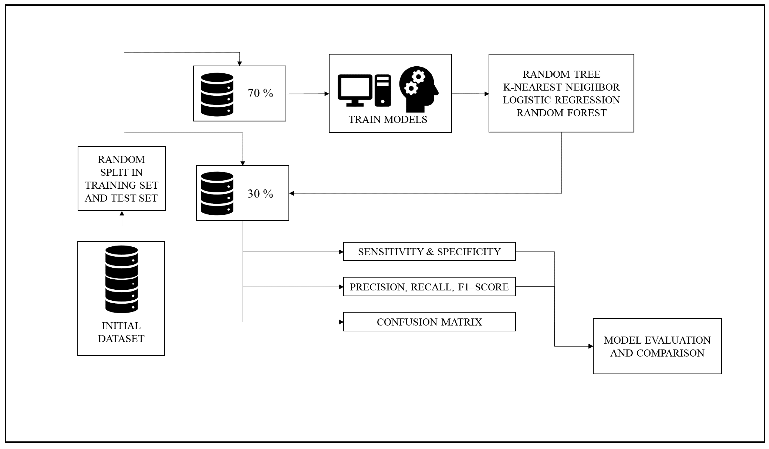
The dataset was randomly split into training and test set; the percentages of 70% for the training set and 30% for the test set were used. The four different MLAs (RT, KNN, LR, and RF) were then trained with the training set. Subsequently, MLAs were employed to predict the crash severity of unknown samples belonging to the test set. A set of performance metrics was computed, and the performance of MLAs compared. Figure 1 below describes the first phase of the methodology.
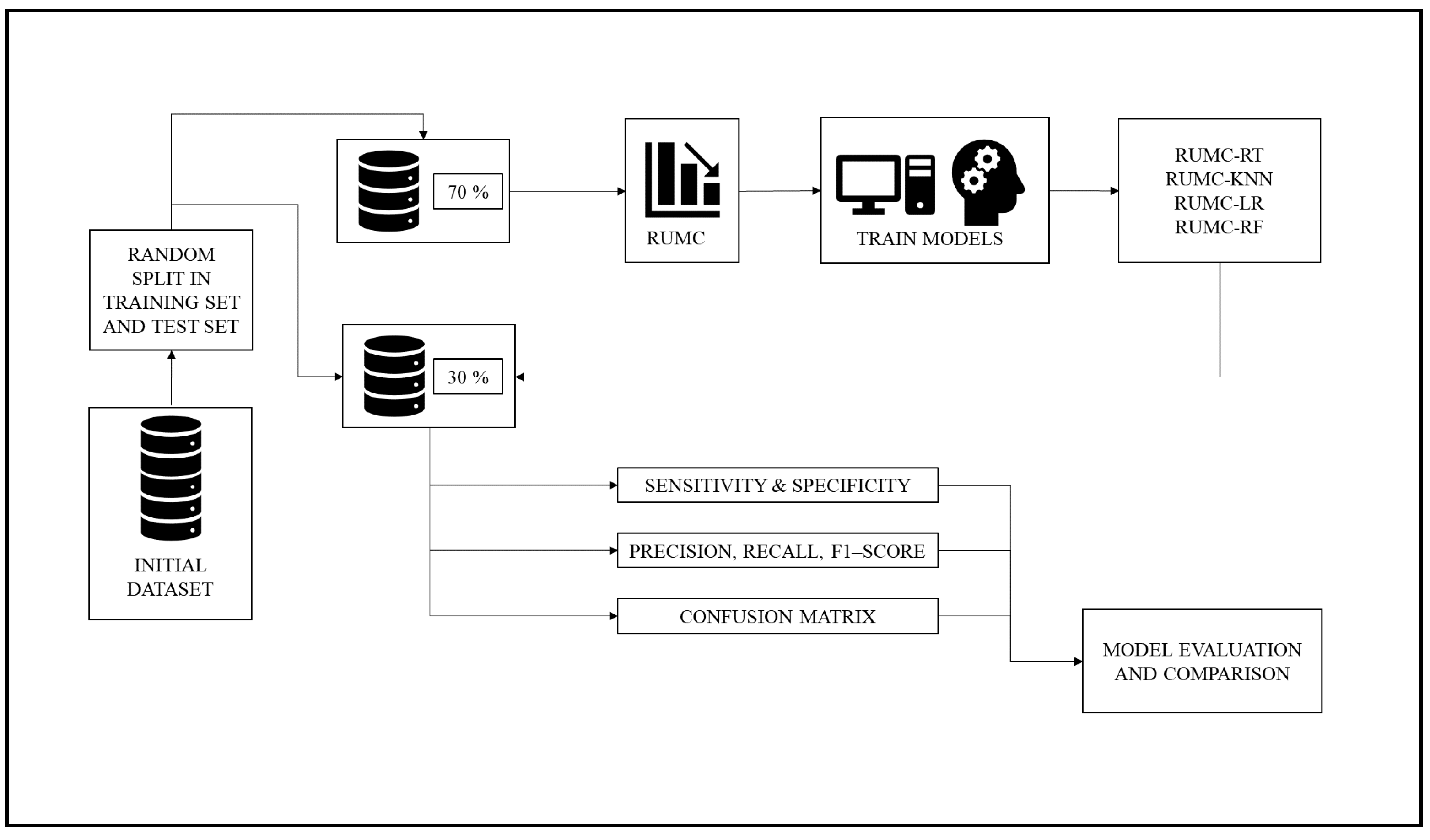
The second phase involves the use of RUMC on the training set before training the MLAs. This operation provides a balanced training set. Once the RUMC is employed, the second phase follows the operations performed in the first one. Finally, we analyzed the outcomes from both phases in order to compare the two models. Figure 2 below shows the second phase of the methodology.
3.2. Input Features
The dataset contains 6515 crash records that occurred on stretches of road and road junctions in York, Great Britain, from 2005 to 2018. For each accident that occurred, a set of 17 different features related to the roadway, user, and vehicle are reported. These features are the input factors (or independent variables) of the MLAs we calibrated. They are reported in Table 2.
3.3. Output Classes
The output (or dependent variable) of the MLAs are crash severity classes. The dataset provides three different crash severity classes: fatal crash, injury crash, and PDO crash. These three classes are significantly imbalanced; indeed, there are 5594 PDO crashes (85.86% of the total amount of crashes), 856 injury crashes (13.14%), and 65 fatal crashes (1%). The initial dataset was defined by aggregating fatal crashes and injury crashes. Other studies [26,28,31,32] merged two or more classes in order to obtain better results. Figure 3 below shows the three crash severity classes (Figure 3a) and the initial dataset containing the new merged class (F + I class) and PDO class (Figure 3b).
Figure 3b confirms that there is still a substantial imbalance between the two classes (ratio of about 1:6).
3.4. Random Undersampling the Majority Class
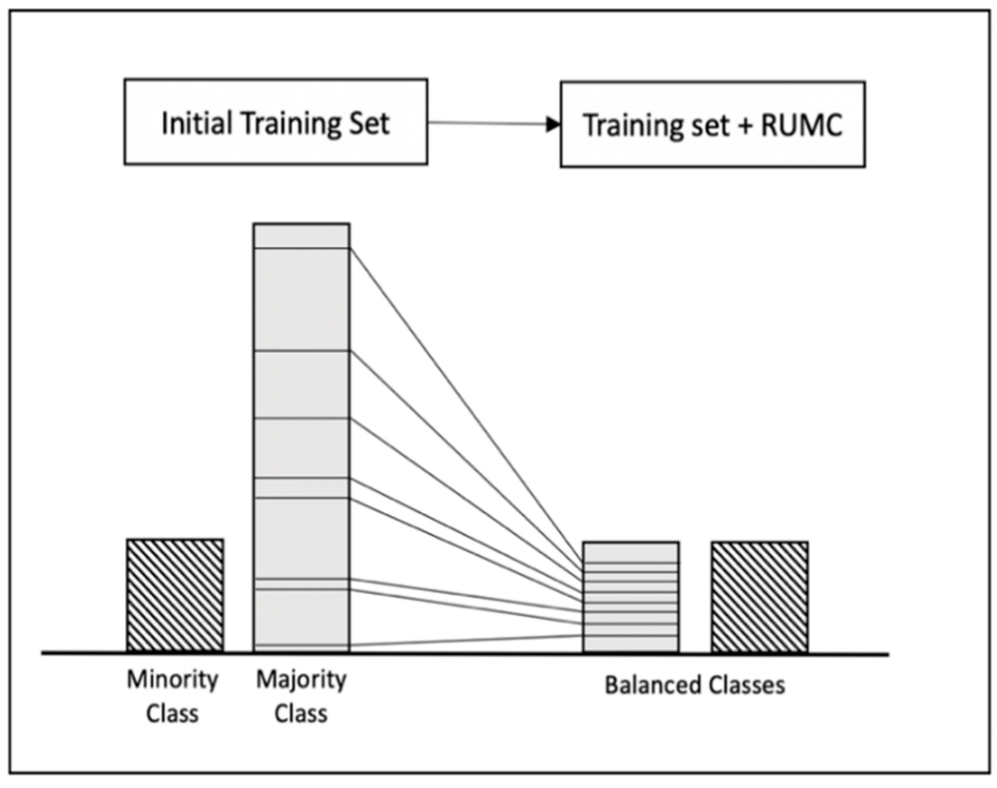
The RUMC technique involves randomly selecting examples from the majority class and removing them for the training dataset. The majority class instances are discarded at random until a balanced class distribution in the training set is reached (Figure 4).
Before implementing RUMC, the dataset contains a minority and majority class. After RUMC, we can deal with a balanced dataset.
3.5. Machine Learning Algorithms
Since we aimed at predicting a crash severity class, MLAs for classification (or classifiers) are the most suitable for achieving our purpose. Classifiers are supervised MLAs employed for assigning a label (or a class) to new unknown observations. In order to predict a class, supervised classifiers are trained using a dataset of already-known observations, i.e., samples in which the input features and output class are provided. Usually, the input feature can be nominal, ordinal, or numerical.
It is worth mentioning that Waikato Environment for Knowledge Analysis (WEKA) software was used [45,46], version 3.8.4, to carry out the modeling.
The classifiers used in this study are now introduced briefly.
3.5.1. Random Tree
In order to introduce the RT, the Classification and Regression Tree (CART) developed by Breiman is described [47]. CART is a hierarchical non-parametric approach that grows a tree-based model by repeatedly splitting the dataset into homogeneous zones. The decision rules for splitting each node are learned by inferring directly from the available data. The recursive partitioning algorithm [47,48] is used to define the decision rules. Once the CART model is trained, the decision rules can be used for predicting the class of new unknown observations.
CART models have been widely used in machine learning modeling due to their advantages:
- They provide an interpretable solution of the predictions using tree graph visualization;
- They provide an automatic variable selection making them insensitive to irrelevant variables, outliers, and the scales of predictors;
- They are computationally efficient even in large problems (generally, low time for training is required), also allowing missing values of the input factors and both numerical and categorical predictors to be handled;
- CART outcomes are unaffected by monotone transformations of the input factors.
However, CART models are prone to overfitting the data by creating over-complex deep trees, and they are sensitive to small changes in the training set: slightly different training sets can lead to significantly different CART models. In order to overcome these issues, the RT provides more robust outcomes than CART models by exploiting the feature randomness approach, i.e., each node of the trees is split into branch nodes using a fixed number of input features, selected at random [49]. In this study, the number of input factors randomly sampled () as candidates at each split is equal to the default value of the WEKA software. The default value was chosen after a “trial & error” approach: indeed, has been fixed to 1, 2, …, 17, identifying the best accuracy by means of a 10-fold Cross-Validation (CV) process for equal to the default value of the WEKA software, as computed in Equation (1) below:
where is the number of input factors. In this study, = 17, and the resulting = 5.
3.5.2. K-Nearest Neighbor
KNN was first defined by Cover and Hart [50]. KNN is an algorithm that aims at classifying an observation by looking at the closest k observations contained in the feature space. The class that belongs to the majority of the k closest observations is taken as the class of the new observation. Therefore, KNN assigns to an unclassified sample point the class of the k nearest set of previously classified points. In the implementation of KNN, two hyperparameters are requested to the modeler: the number of the k nearest neighbors and the distance function to employ to define a distance metric between observations into the feature space:
- The number of neighbors should be determined by trying different values of k and finding the best accuracy of the classifier after a 10-fold CV process. Considering this, we tried k = 1, 2, 5, 10, 15, 20, and 25. We chose k = 1 considering the highest accuracy;
- The Euclidean distance was employed as a distance function to compute the distance between observations. The Euclidean distance between two points, i and j, is defined as:where:
- m is the dimension of the points (i.e., the number of independent variables);
- and are the values of the k-th independent variable for observations i and j, respectively.
3.5.3. Logistic Regression
LR classifier was introduced by Berkson [51] and quickly became one of the most employed algorithms for classification purposes. LR firstly involves a linear multivariate regression between the output (or dependent variable) and input factors (or independent variables). Subsequently, the output of the multivariate regression is passed by a logit function, leading to a numerical output within the range [0, 1]. Indeed, the logit function is a sigmoid function (i.e., S-shaped) that outputs a number between 0 and 1. Equation (3) below defines the logit function.
where:
P(z) is the probability of an occurrence (crash severity) that varies from 0 to 1; Equation (4) below defines z, which is the dependent variable of the linear multivariate regression.
where:
- is a constant term;
- m is the number of independent variables;
- (i = 1, 2, 3, …, n) represents the value of the i-th input factor;
- (i = 1, 2, 3, …, n) is the regression coefficient assigned to the i-th input factor.
Once the probability P(z) has been computed, the LR classifier makes its prediction as follows (Equation (5)):
Moreover, the regression coefficients determined in the logistic regression can be interpreted as a measure of the relative importance of the independent variables.
3.5.4. Random Forest
Breiman [52] introduced the RF classifier. RF consists of a large number of individual and uncorrelated decision trees that operate as an ensemble classifier to formulate a prediction. In order to obtain uncorrelated trees, they are assembled using a bootstrap aggregation (Bagging) approach, i.e., creating a subset of training samples through replacement. The algorithm exploits two-thirds of the samples (called in-bag samples) to train the trees, while it employs the remaining one third (called out-of-bag samples) in an internal CV procedure. The CV is used by the algorithm to minimize the error estimation, called the out-of-bag error, and to grow the most reliable RF. There is no pruning procedure in the definition of the decision trees. Moreover, RF exploits the feature randomness approach. By growing the RF with a large number of trees, the algorithm creates trees that have high variance and low bias.
Once the RF has grown, it can predict the class of a new observation by averaging the class assignment by all the decision trees: each decision tree votes for a class and the class with the maximum votes is the selected one for the new observation.
In the implementation of RF, two hyperparameters are requested to the modeler:
- The number of decision trees, , to grow: since RF does not overfit the data, the number of decision trees can be as large as possible. However, the higher the number of trees, the higher is the time required for growing the RF. We fixed different values of , specifically, 10, 25, 50, 100, 200, 400, 800, and 1000, evaluated using a 10-fold CV the goodness-of-fit of the models. We chose = 100 trees since a higher number did not produce a significant increase in RF performance, requiring a massive amount of time for training instead.
- The number of input factors randomly sampled, , as candidates at each split: in this study, as for the RT algorithm, was chosen after a “trial & error” approach; indeed, has been fixed to 1, 2, …, 17, identifying the best accuracy by means of a 10-fold CV process for equal to the default value of the WEKA software. Therefore, we also chose for RT, = 5.
3.6. Predictor Importance
The RF algorithms allowed the importance of each input factor in predicting crash severity to be evaluated. The leading relations for computing the predictor importance are reported below. Readers can find a comprehensive explanation of the procedure in Breiman [52] and Louppe et al. [53]. We remind the reader that a tree, T, is trained by exploiting a sample of N observations, using the recursive partitioning algorithm [47,48]. This algorithm identifies at each node, t, the best split, , (i.e., the feature chosen for splitting the node and the best cut point) for partitioning the node samples into and branch node samples, maximizing the decrease, , of an impurity measure, . Trees end at leaf nodes when nodes become pure (all the observations belong to the same class) or when an error threshold is reached. The impurity decrease is computed using Equation (6).
where:
In this study, the impurity, i(t), at the node, t, is represented by the Gini index as follows (Equation (7)):
where:
- j represents the output class;
- is the posterior probability that a sample belongs to class j given that it lies in t.
In RF modeling, Breiman [52] suggested evaluating the importance of an independent input variable, , to predict the output class by adding up the weighted impurity decreases, , for all nodes, t, when is used for splitting the nodes, averaged over all trees in the forest (Equation (8)).
where:
- is the importance of the variable ;
- is the proportion of samples reaching the node t;
- is the independent variable used in split .
3.7. K-Fold Cross Validation Procedure
The concept of CV was introduced first in the study of Larson [54]. The author split the dataset into two parts: the first one was used for building the regressor and the second one for testing the algorithm. The current k-fold CV procedure appeared subsequently in the book of Mosteller and Turkey [55]. CV is a method for training, evaluating, or comparing MLAs by distributing data into two sets: one employed for training the model and the other for validating the model [56]. Frequently, CV assumes the structure of k-fold CV, where the training set is cut into k folds of the same dimension. Therefore, there are k iterations of training and validation. At each iteration, k-1 folds are used for learning, while the remaining fold is used to validate the model. Accordingly, after the CV process, each sample has been used both for training and for testing.
Furthermore, to guarantee that each fold is representative of the complete dataset, data is stratified before being split into folds. A stratification technique prepares the data such that, in every fold, each class is represented by its real percentage in respect to the other classes. Kohavi [57] recommended stratified 10-fold CV as the best model selection procedure. Several other studies [5,15,21,22,32] used k-fold CV. Therefore, we followed a 10-fold CV procedure to train all the mentioned MLAs, by employing all the possible combination of hyperparameters aforementioned. Once the models had been trained with the best set of hyperparameters, we assessed them by computing their performance on the test set.
3.8. Performance Metrics
As said, a large set of performance metrics allows MLAs to be comprehensively evaluated and compared to each other. Equations (9)–(14) define the overall accuracy of the classifier and the precision, TPR, FPR, TNR, and F1-score.
where:
- TP is the number of True Positive instances, i.e., the instances belonging to class 1 correctly classified into the same class;
- TN is the number of True Negative instances, i.e., the instances belonging to the class 0 correctly classified into the same class;
- FP is the number of False Positive instances, i.e., the instances belonging to the class 0 erroneously classified into class 1;
- FN is the number of False Negative instances, i.e., the instances belonging to the class 1 erroneously classified into class 0;
It is worth noting here that class 1 represents the F + I class, while class 0 represents the PDO class. The overall accuracy of the classifier aims to represent the global performance of the classifier. The precision shows the goodness of positive predictions. The TPR, or recall, is the ratio of positive instances that are correctly detected by the classifier. Analogously, the TNR is the ratio of negative instances correctly detected by the classifier. The FPR is the ratio of FP among all negative instances, i.e., the percentage of “false alarms”. The F1-score is the harmonic mean of precision and recall, and it can be used to compare classifiers since it combines two metrics into a more concise one. Precision, TPR, FPR, TNR, and F1-score can be computed as specific metrics for each class or as the overall metrics of the classifier. Finally, we computed the confusion matrix. It reports the TP, TN, FP, and FN as a matrix, in which the rows correspond to the observed (or actual) classes, while the columns correspond to the predicted classes. A satisfactory confusion matrix should have most of the instances on its main diagonal.
4. Results and Discussion
4.1. Imbalanced and RUMC-Based Training Sets
Figure 5 below reports the training sets and test set. Figure 5a shows the random split into training (70%) and test set (30%), while Figure 5b shows the RUMC-based training set.
We observed an imbalance ratio of 1:6 in the training set of Figure 6a. The RUMC-based training set is balanced correctly instead.
4.2. Performance of the Algorithms
Below, we report the performance of the models on the test set in terms of:
- TPR, FPR, and TNR: Table 3 shows the performance of the models trained by the imbalanced training set (namely RT, KNN, LR, and RF), while Table 6 shows the performance of the RUMC-based model (namely RUMC-RT, RUMC-KNN, RUMC-LR, and RUMC-RF). Both tables report the performance for F + I class, PDO class, and the weighted average performance of the classifier, which is the average of both values weighted by the number of instances in each class of the test set.
- Precision, recall, and F1 score: Table 4 shows the performance of the models trained by the imbalanced training set, while Table 7 shows the performance of the RUMC-based model; both tables report the performance for F + I class, PDO class, and the weighted average performance of the classifier;
- Confusion matrix and overall accuracy: Table 5 shows the confusion matrices of the models trained by the imbalanced training set, while Table 8 shows the confusion matrices of the RUMC-based model. The overall accuracy is presented in terms of the number of correctly classified instances. We also report the number and percentage of incorrectly classified instances.
Although TPR and recall have the same meaning, we report both since TPR is usually presented along with FPR, while precision is commonly accompanied by recall.
4.2.1. Algorithms Trained by the Imbalanced Training Set
As expected, Table 3 shows that the algorithms present a satisfactory weighted average performance both for TPR and FPR. Indeed, the TPR ranges from 78.5% (KNN) to 85.7% (LR), while FPR varies from 78.5% (KNN) to 85.8% (LR). However, by observing the specific performance for each class, we can confirm that the classifiers are weak in predicting the F + I class. Indeed, TPR ranges from 0% (LR) to 18.3% (KNN), while FPR varies from 0.1% (LR) to 11.5% (KNN). Judging a classifier by assessing the performance for each class seems to be the most suitable and reliable method.
Furthermore, the TNR values denote that the classifier can accurately identify the TN instances when the class examined is the F + I class (i.e., the TN instances belong to the PDO class). In contrast, the classifier is weak at correctly recognizing TN instances when the PDO class is under consideration. TNR represents an additional confirmation that the high percentage of the majority class strongly affects the prediction capabilities of the minority class by the classifiers.
Table 4 below reports the precision, recall, and F1 score of the models trained by the imbalanced training set.
Table 4 introduces another set of performance metrics that seem to confirm the outcomes of Table 3. Indeed, by observing the weighted average precision, recall, and F1 score, we may expect good classifiers. On the contrary, by examining the metrics specified for each class, the weakness in predicting the minority class of the classifier is manifest. Accordingly, when the metrics chosen for introducing a classifier are precision, recall, and F1 score, we still should consider the specific performance for each class.
Table 5 below reports the confusion matrices and the overall accuracy for RT, KNN, LR, and RF. The main diagonal of each confusion matrix appears in bold.
Since the confusion matrix reports the comparison between the number of observed instances correctly and incorrectly classified for each class, it seems an appropriate performance metric for introducing a classifier. Moreover, using Equations (9)–(14), all the other performance metrics can be computed. By observing Table 5, we can judge KNN as the best classifier for predicting F + I class (51 out of 278 instances correctly detected), followed by RT (43 out of 278), RF (16 out of 278), and LR (0 out of 278). As for the PDO class, the best classifier is the LR (1677 out of 1678), followed by RF (1631 out of 1678), RT (1498 out of 1678), and KNN (1485 out of 1678).
Considering the overall accuracy, LR seems the best classifier (85.74%), followed by RF (83.38%), RT (78.78%), and KNN (78.53%). Confusion matrices clearly demonstrate that the accuracy is an untrustworthy metric for evaluating the MLA calibrated using an acutely imbalanced dataset. Indeed, the accuracy simply follows the prior percentages of the classes. For instance, the LR (which resulted in the best MLA with an accuracy of 85.74%) simply provides the same prediction for practically all the instances (1955 out of 1956), i.e., it classifies each instance as PDO crash. Considering the percentage of the classes, LR provides the right prediction in 1677 cases, thus the resulting high, but unreal, accuracy. The same considerations can be addressed for all the other MLAs.
4.2.2. Performance of RUMC-Based Algorithms
Table 6 introduces the trade-off that exists between TPR and FPR. Indeed, using a balanced training set, we note a decrease in performance for predicting PDO class and a significant increase in performance related to the F + I class. In the case of RUMC-based models, the ratio of positive instances correctly detected by the classifier (TPR) increases, while the ratio of negative instances correctly detected by the classifier (TNR) decreases. For the real application of such models by companies, this is reflected in a more accurate prediction about fatal accidents or those causing injury and a certain number of false alarms (the FP instances) that are mistakenly classified as severe. Anyhow, for these companies, it is certainly more important that TPR and FPR take on this type of trade-off than that shown in Table 3. The average weighted performances are lower than those of Table 3, reflecting a more balanced trade-off between the performance of each class. Again, these evaluation metrics are not able to consistently represent a classifier.
Table 7 reports the precision, recall, and F1 score of the RUMC-based model.
Table 7 shows that the precision for the PDO class is still high. Compared with Table 4, the precision for the F + I Class is slightly lower for RUMC-RT, RUMC-KNN, and RUMC-RF, while it is significantly increased for RUMC-LR. The recall for the PDO class is decreased, and consequently, we note a significant improvement in recall for the F + I class. As observed for TPR and FPR, there is a trade-off between precision and recall. The F1 score is improved in the F + I class and is decreased in the PDO class. Again, the weighted average metrics do not seem appropriate in describing such classifiers.
Table 8 reports the confusion matrices and the overall accuracy for RUMC-based algorithms.
By observing Table 8 above, we can confirm the significant increase in classifier performance brought by the RUMC technique. Indeed, the classifiers are now able to predict satisfying both the F + I and PDO class. The best classifiers in predicting F + I crashes are RUMC-RT and RUMC-KNN (159 out of 278), followed by RUMC-RF (158 out of 278), and RUMC-LR (146 out of 278). As regards the PDO class, the classifier with the best performance is the RUMC-LR (1077 out of 1678), followed by RUMC-RF (940 out of 1678), RUMC-RT (838 out of 1678), and RUMC-KNN (789 out of 1678). The higher overall accuracy is reached by RUMC-LR (62.53%), followed by RUMC-RF (56.14%), RUMC-RT (50.97%), and RUMC-KNN (48.47%). Since the dataset is now balanced, the accuracy should adequately represent the overall performance of the classifiers. Considering this, it seems that the best one is the LR; however, that is not to say that the best overall performance always corresponds to the best model to be employed. Indeed, it depends on the scope for which the MLAs will be used. Probably, in the present case, managing bodies and road authorities are more interested in the best prediction of severe accidents (therefore, they may prefer KNN or RT). Thus, specific performance metrics for each class, such as the number of F + I or the number of PDO crashes correctly predicted, are more interesting and useful for choosing the MLAs to be used rather than relying on overall performance metrics.
For application purposes for which these MLAs are designed, the RUMC-based models were the most suitable, considering that they identify the minority class (F + I class) with greater accuracy. Surely, considering the needs of the companies that could use these models, this class is the most relevant of the two severity classes. Having some false alarms (as evidenced by Table 6–8) should not lead to significant issues in the planning duties of these companies. Indeed, it is more appropriate to examine a false alarm more carefully than to predict a fatal accident such as a PDO accident. Only by consistently recognizing severe accidents (and therefore, the factors that caused them) is it possible to provide adequate planning aimed at reducing and correctly handling the crash severity.
4.3. Predictor Importance
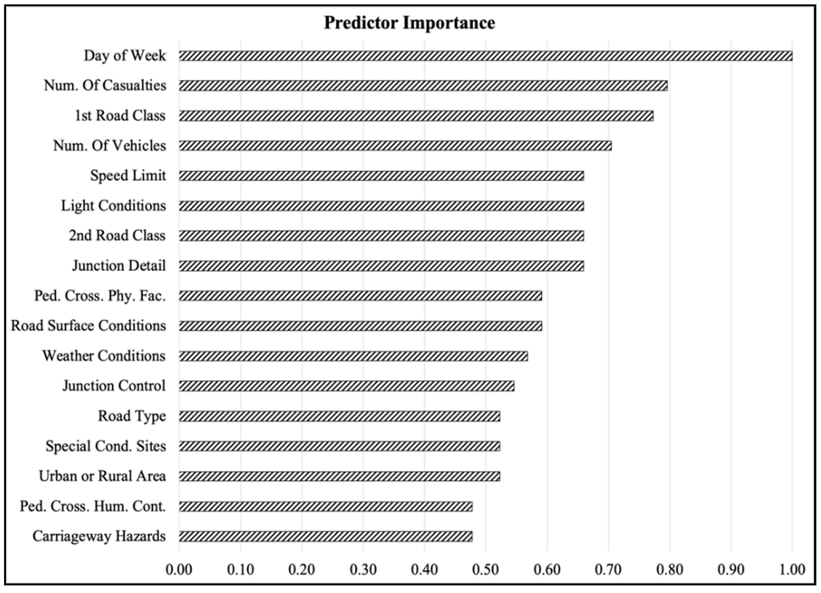
Relying on the Gini index impurity decrease, the importance of each input factor has been computed. For the sake of clarity, Figure 6 shows the standardized predictor importance, which is the predictor importance calculation rearranged in the range [0, 1].
Figure 6 demonstrates that each input factor has significant importance in determining crash severity since they are all greater than zero. Qualitatively, we can distinguish three leading families among the inputs: high-importance input features, medium-importance input features, and low-importance input features. The term “importance” refers to how much an input factor affects or is associated with the crash severity.
In the high-importance set of input features lie the day of the week, the number of casualties, the first road class, and the number of vehicles. While it was intuitive that the first road class, the number of casualties, and the number of vehicles could have been significant in modeling crash severity, the same cannot be said for the “Day of the Week” factor. This parameter is entirely independent of the factors associated with the infrastructure, circulation, and type of vehicles but is mainly related to user behavior during the week. Table 9 below shows some data obtained by analyzing the change in crashes as a function of the day of the week.
Table 9 demonstrates that there are significant changes in the number of accidents and the crash severity during the week. Friday seems to be the day in which most of the accidents occur (1123 accidents, corresponding to 17.24% of the total), while Sunday is the day when least accidents happen, with 628 accidents (9.64% of the total). As regards the severity, Friday is the most severe day, with 159 out of 921 F + I crashes (17.26% of the total) and 964 out of 5594 PDO crashes (17.23% of the total). Contrary to overall percentages, Sunday appears to be the most dangerous day, with a probability of 17.99% to be involved in a fatal crash or one causing injury. Tuesday is the day when an accident is more likely to be of the PDO type (probability of 87.56%). These day-to-day changes confirm that the “Day of the week” parameter is essential in assessing the crash severity.
The medium-importance set of input features contains the speed limit, the light conditions, the second road class, and the junction detail. The speed limit may be significant since it is correlated to the road class, while the second road class and junction detail are significant since 3853 out of 6515 crashes occurred at a junction. Therefore, the evaluation of the second road class and the type of junction should be essential in predicting crash severity.
The low-importance set of input features contains all the other input factors.
With a view to road traffic planning by a national road authority, it should, therefore, be appropriate to provide more checks by law enforcement and surveillance over the weekend, or the installation of speed control systems in critical situations should be envisaged. Furthermore, the proper regulation of junctions between roads could alleviate the number of fatal accidents in favor of PDO accidents, as well as mitigate their number.
4.4. Future Works
In order to further improve the present research, additional future works could implement the latest available machine and deep learning models on the same dataset analyzed. For instance, we want to mention some road safety analyses using different types of neural networks that could be implemented: multilayer perceptron neural networks [14,27,29], convolutional neural networks [28,40,58], radial basis function neural networks [25], recurrent neural networks [59], and deep Neural networks [10,18,58]. Moreover, other ensemble of learners (in addition to the RF algorithm calibrated in the present study) [9,16] and the staking [32] strategy could also be considered. Having a broad set of calibrated algorithms available, it would be possible to accurately identify the best one for predicting crash severity in the case of highly imbalanced observations.
A further enhancement that could be made is the verification of the algorithms calibrated in this paper on supplementary datasets, in order to confirm whether the test phase carried out provides the real reliability of the models.
5. Conclusions
The paper aimed to predict road crash severity by employing MLAs. We suggested a procedure for handling imbalanced accident datasets in order to predict the minority crash severity class appropriately. Below, the main findings and the methodology are briefly recapped.
Firstly, a comprehensive literature review related to crash severity prediction using MLAs was carried out: a noticeable number of recent papers in which the authors used MLAs relying on an acutely imbalanced dataset was found. These algorithms have satisfactory performance in predicting the majority class (e.g., PDO crashes,) and poor performance in predicting the minority class (e.g., fatal or injury crashes). For the purposes for which such MLAs should be used, the minority class assumes generally greater importance than the majority one. Therefore, oversampling and undersampling techniques have been introduced in order to handle imbalanced datasets, along with the reasons why the RUMC has been followed in the present paper.
The available dataset was split randomly into a training and test set; an RUMC approach was applied to the training set to provide a new balanced one. Therefore, two types of MLAs were trained onto these two different sets using a 10-Fold CV. Four algorithms trained on the imbalanced training set (RT, KNN, LR, and RF) and four algorithms trained on RUMC-based training set (RUMC-RT, RUMC-KNN, RUMC-LR, and RUMC-RF) are provided. Both types of algorithms were tested on the same test set, allowing us to compare the outcomes and evaluating our suggested procedure. A broad set of performance metrics, including TPR, FPR, TNR, precision, recall, overall accuracy, and the confusion matrix, was computed for each algorithm. We showed that metrics related to specific classes are more representative of the real performance of the classifier than overall metrics. Moreover, it seems that the confusion matrix is the most appropriate and suitable representation for describing the predictive capacities of a classifier. We also showed that accuracy is untrustworthy metric if it is computed for MLAs trained on imbalanced datasets.
As regards the performance of the algorithms, the RUMC-based models showed better predictive capabilities in detecting the minority class than the algorithms trained by the imbalanced dataset. The best classifiers in predicting fatal crashes and those causing injury are RUMC-RT and RUMC-KNN (159 samples out of 278 correctly identified), followed by RUMC-RF (158 out of 278), and RUMC-LR (146 out of 278). As regards the PDO class, the classifier with the best performance is the RUMC-LR (1077 samples out of 1678 correctly identified), followed by RUMC-RF (940 out of 1678), RUMC-RT (838 out of 1678), and RUMC-KNN (789 out of 1678). The higher overall accuracy is reached by the RUMC-LR (62.53%), followed by RUMC-RF (56.14%), RUMC-RT (50.97%), and RUMC-KNN (48.47%).
Finally, the importance of each input factor was computed using the average Gini index impurity decrease. All the input factors have significant importance in predicting crash severity. The most relevant input factors are day of the week, number of vehicles, casualties involved, and the first road class.
Relying on all these findings, we can conclude by asserting that the use of balanced MLAs is recommended as a promising tool for crash severity modeling and prediction. The use of balanced datasets appears to be essential for correctly predicting accidents with higher severity. National road authorities, insurance companies, hospitals, and all the other companies interested in crash severity can make use of MLAs and the RUMC technique for managing their duties properly.
Author Contributions
N.F. was involved in the conceptualization, methodology, software, validation, resources, investigation, data curation, writing—original draft, visualization, and formal analysis. M.L. was involved in validation, resources, writing—review and editing, supervision, and project administration. All authors have read and agreed to the published version of the manuscript.
Funding
This research received no external funding.
Acknowledgments
Data were provided by the United Kingdom Open Data Portal (UK Government, Department for Transport), https://data.gov.uk/, which contains public sector information licensed under the Open Government Licence v3.0, http://www.nationalarchives.gov.uk/doc/open-government-licence/version/3/.
Conflicts of Interest
The authors declare no conflicts of interest.
References
- World Health Organization. Global Status Report on Road Safety 2018: Summary 2018; World Health Organization: Geneva, Switzerland, 2018.
- Cateni, S.; Colla, V.; Vannucci, M. A method for resampling imbalanced datasets in binary classification tasks for real-world problems. Neurocomputing 2014, 135, 32–41. [Google Scholar] [CrossRef]
- He, H.; Garcia, E.A. Learning from imbalanced data. IEEE Trans. Knowl. Data Eng. 2009. [Google Scholar] [CrossRef]
- Japkowicz, N.; Stephen, S. The class imbalance problem: A systematic study. Intell. Data Anal. 2002. [Google Scholar] [CrossRef]
- Zhang, J.; Yang, J. Instance-Based Learning for Highway Accident Frequency Prediction. Comput. Civ. Infrastruct. Eng. 1997, 12, 287–294. [Google Scholar] [CrossRef]
- Singh, G.; Sachdeva, S.N.; Pal, M. Support vector machine model for prediction of accidents on non-urban sections of highways. Proc. Inst. Civ. Eng. Transp. 2018, 171, 253–263. [Google Scholar] [CrossRef]
- Singh, G.; Sachdeva, S.N.; Pal, M. M5 model tree based predictive modeling of road accidents on non-urban sections of highways in India. Accid. Anal. Prev. 2016, 96, 108–117. [Google Scholar] [CrossRef] [PubMed]
- Tang, H.; Donnell, E.T. Application of a model-based recursive partitioning algorithm to predict crash frequency. Accid. Anal. Prev. 2019, 132, 105274. [Google Scholar] [CrossRef]
- Zhang, X.; Waller, S.T.; Jiang, P. An ensemble machine learning-based modeling framework for analysis of traffic crash frequency. Comput. Civ. Infrastruct. Eng. 2020, 35, 258–276. [Google Scholar] [CrossRef]
- Singh, G.; Pal, M.; Yadav, Y.; Singla, T. Deep neural network-based predictive modeling of road accidents. Neural Comput. Appl. 2020, 1–10. [Google Scholar] [CrossRef]
- Li, X.; Lord, D.; Zhang, Y.; Xie, Y. Predicting motor vehicle crashes using Support Vector Machine models. Accid. Anal. Prev. 2008, 40, 1611–1618. [Google Scholar] [CrossRef]
- Abdel-Aty, M.; Haleem, K. Analyzing angle crashes at unsignalized intersections using machine learning techniques. Accid. Anal. Prev. 2011, 43, 461–470. [Google Scholar] [CrossRef] [PubMed]
- Harb, R.; Yan, X.; Radwan, E.; Su, X. Exploring precrash maneuvers using classification trees and random forests. Accid. Anal. Prev. 2009, 41, 98–107. [Google Scholar] [CrossRef]
- Wang, J.; Kong, Y.; Fu, T. Expressway crash risk prediction using back propagation neural network: A brief investigation on safety resilience. Accid. Anal. Prev. 2019, 124, 180–192. [Google Scholar] [CrossRef]
- Delen, D.; Tomak, L.; Topuz, K.; Eryarsoy, E. Investigating injury severity risk factors in automobile crashes with predictive analytics and sensitivity analysis methods. J. Transp. Heal. 2017, 4, 118–131. [Google Scholar] [CrossRef]
- Xiao, J. SVM and KNN ensemble learning for traffic incident detection. Phys. A Stat. Mech. its Appl. 2019, 517, 29–35. [Google Scholar] [CrossRef]
- Schlögl, M.; Stütz, R.; Laaha, G.; Melcher, M. A comparison of statistical learning methods for deriving determining factors of accident occurrence from an imbalanced high resolution dataset. Accid. Anal. Prev. 2019, 127, 134–149. [Google Scholar] [CrossRef]
- Theofilatos, A.; Chen, C.; Antoniou, C. Comparing Machine Learning and Deep Learning Methods for Real-Time Crash Prediction. Transp. Res. Rec. 2019, 2673, 169–178. [Google Scholar] [CrossRef]
- Chen, Q.; Song, X.; Yamada, H.; Shibasaki, R. Learning deep representation from big and heterogeneous data for traffic accident inference. In Proceedings of the Thirtieth AAAI Conference on Artificial Intelligence, Phoenix, AZ, USA, 12–17 February 2016; pp. 338–344. [Google Scholar]
- Dogru, N.; Subasi, A. Traffic accident detection using random forest classifier. In Proceedings of the 2018 15th Learning and Technology Conference, L and T 2018, Jeddah, Saudi Arabia, 25–26 February 2018; Institute of Electrical and Electronics Engineers Inc.: Piscataway, NJ, USA, 2018; pp. 40–45. [Google Scholar]
- Al Mamlook, R.E.; Kwayu, K.M.; Alkasisbeh, M.R.; Frefer, A.A. Comparison of machine learning algorithms for predicting traffic accident severity. In Proceedings of the 2019 IEEE Jordan International Joint Conference on Electrical Engineering and Information Technology (JEEIT), Amman, Jordan, 9–11 April 2019; pp. 272–276. [Google Scholar] [CrossRef]
- Mokhtarimousavi, S.; Anderson, J.C.; Azizinamini, A.; Hadi, M. Improved Support Vector Machine Models for Work Zone Crash Injury Severity Prediction and Analysis. Res. Artic. Transp. Res. Rec. 2019, 2673, 680–692. [Google Scholar] [CrossRef]
- Abellán, J.; López, G.; De Oña, J. Analysis of traffic accident severity using Decision Rules via Decision Trees. Expert Syst. Appl. 2013, 40, 6047–6054. [Google Scholar] [CrossRef] [Green Version]
- Chang, L.Y.; Wang, H.W. Analysis of traffic injury severity: An application of non-parametric classification tree techniques. Accid. Anal. Prev. 2006, 38, 1019–1027. [Google Scholar] [CrossRef] [PubMed]
- Abdelwahab, H.T.; Abdel-Aty, M.A. Development of artificial neural network models to predict driver injury severity in traffic accidents at signalized intersections. Transp. Res. Rec. 2001, 6–13. [Google Scholar] [CrossRef]
- Chen, C.; Zhang, G.; Qian, Z.; Tarefder, R.A.; Tian, Z. Investigating driver injury severity patterns in rollover crashes using support vector machine models. Accid. Anal. Prev. 2016, 90, 128–139. [Google Scholar] [CrossRef]
- Alkheder, S.; Taamneh, M.; Taamneh, S. Severity Prediction of Traffic Accident Using an Artificial Neural Network. J. Forecast. 2017, 36, 100–108. [Google Scholar] [CrossRef]
- Iranitalab, A.; Khattak, A. Comparison of four statistical and machine learning methods for crash severity prediction. Accid. Anal. Prev. 2017, 108, 27–36. [Google Scholar] [CrossRef]
- Wahab, L.; Jiang, H. Severity prediction of motorcycle crashes with machine learning methods. Int. J. Crashworthiness 2019. [Google Scholar] [CrossRef]
- Zhang, J.; Li, Z.; Pu, Z.; Xu, C. Comparing prediction performance for crash injury severity among various machine learning and statistical methods. IEEE Access 2018. [Google Scholar] [CrossRef]
- Li, Z.; Liu, P.; Wang, W.; Xu, C. Using support vector machine models for crash injury severity analysis. Accid. Anal. Prev. 2012, 45, 478–486. [Google Scholar] [CrossRef]
- Tang, J.; Liang, J.; Han, C.; Li, Z.; Huang, H. Crash injury severity analysis using a two-layer Stacking framework. Accid. Anal. Prev. 2019, 122, 226–238. [Google Scholar] [CrossRef]
- Krishnaveni, S.; Hemalatha, M. A perspective analysis of traffic accident using data mining techniques. Int. J. Comput. Appl. 2011, 23, 40–48. [Google Scholar] [CrossRef]
- Yu, Q.; Zhou, Y. Traffic safety analysis on mixed traffic flows at signalized intersection based on Haar-Adaboost algorithm and machine learning. Saf. Sci. 2019. [Google Scholar] [CrossRef]
- Yuan, J.; Abdel-Aty, M.A.; Yue, L.; Cai, Q. Modeling Real-Time Cycle-Level Crash Risk at Signalized Intersections Based on High-Resolution Event-Based Data. IEEE Trans. Intell. Transp. Syst. 2020. [Google Scholar] [CrossRef]
- Wu, K.-F.; Nashir Ardiansyah, M.; Ye, W.-J. An evaluation scheme for assessing the effectiveness of intersection movement assist (IMA) on improving traffic safety. Traffic Inj. Prev. 2018, 19, 179–183. [Google Scholar] [CrossRef] [PubMed]
- Lee, C.; Abdel-Aty, M. Comprehensive analysis of vehicle-pedestrian crashes at intersections in Florida. Accid. Anal. Prev. 2005. [Google Scholar] [CrossRef]
- Macioszek, E. Analysis of Driver Behaviour at Roundabouts in Tokyo and the Tokyo Surroundings. In Scientific and Technical Conference Transport Systems Theory and Practice; Springer: Cham, Switzerland, 2019; pp. 216–227. [Google Scholar]
- Basso, F.; Basso, L.J.; Bravo, F.; Pezoa, R. Real-time crash prediction in an urban expressway using disaggregated data. Transp. Res. Part C Emerg. Technol. 2018. [Google Scholar] [CrossRef]
- Li, P.; Abdel-Aty, M.; Yuan, J. Real-time crash risk prediction on arterials based on LSTM-CNN. Accid. Anal. Prev. 2020. [Google Scholar] [CrossRef]
- Zhao, Y.; Cen, Y. Data Mining Applications with R; Academic Press: Cambridge, MA, USA, 2013; ISBN 9780124115118. [Google Scholar]
- Chawla, N.V.; Bowyer, K.W.; Hall, L.O.; Kegelmeyer, W.P. SMOTE: Synthetic minority over-sampling technique. J. Artif. Intell. Res. 2002, 16, 321–357. [Google Scholar] [CrossRef]
- Japkowicz, N. The Class Imbalance Problem: Significance and Strategies. In Proceedings of the 2000 International Conference on Artificial Intelligence (ICAI), Las Vegas, NV, USA, 12–15 July 2010. [Google Scholar]
- Batista, G.E.A.P.A.; Prati, R.C.; Monard, M.C. A study of the behavior of several methods for balancing machine learning training data. ACM SIGKDD Explor. Newsl. 2004. [Google Scholar] [CrossRef]
- Witten, I.H.; Frank, E.; Hall, M.A.; Pal, C.J. The WEKA Workbench. Online Appendix for “Data Mining: Practical Machine Learning Tools and Techniques”; Morgan Kaufmann: Burlington, MA, USA, 2016. [Google Scholar]
- Hall, M.; Frank, E.; Holmes, G.; Pfahringer, B.; Reutemann, P.; Witten, I.H. The WEKA data mining software. ACM SIGKDD Explor. Newsl. 2009, 11, 10. [Google Scholar] [CrossRef]
- Breiman, L.; Friedman, J.H.; Olshen, R.A.; Stone, C.J. Classification and Regression Trees; CRC Press: Belmont, CA, USA, 1984. [Google Scholar]
- Loh, W.-Y.; Shih, Y.-S. Split selection methods for classification trees. Stat. Sin. 1997, 815–840. [Google Scholar]
- Pfahringer, B. Random Model Trees: An Effective and Scalable Regression Method; University of Waikato: Waikato, New Zealand, 2010. [Google Scholar]
- Cover, T.M.; Hart, P.E. Nearest Neighbor Pattern Classification. IEEE Trans. Inf. Theory 1967, 13, 21–27. [Google Scholar] [CrossRef]
- Berkson, J. Application of the Logistic Function to Bio-Assay. J. Am. Stat. Assoc. 1944. [Google Scholar] [CrossRef]
- Breiman, L. Random forests. Mach. Learn. 2001. [Google Scholar] [CrossRef] [Green Version]
- Louppe, G.; Wehenkel, L.; Sutera, A.; Geurts, P. Understanding variable importances in Forests of randomized trees. In Proceedings of the Advances in Neural Information Processing Systems, Lake Tahoe, NV, USA, 5–8 December 2013. [Google Scholar]
- Larson, S.C. The shrinkage of the coefficient of multiple correlation. J. Educ. Psychol. 1931, 22, 45–55. [Google Scholar] [CrossRef]
- Mosteller, F.; Tukey, J.W. Data Analysis, Including Statistics. In The Handbook of Social Psychology; Addison-Welsey: Boston, MA, USA, 1968; Volume 2, pp. 80–203. [Google Scholar]
- Refaeilzadeh, P.; Tang, L.; Liu, H. Cross-Validation. In Encyclopedia of Database Systems; Springer: New York, NY, USA, 2016. [Google Scholar]
- Kohavi, R. A Study of Cross-Validation and Bootstrap for Accuracy Estimation and Model Selection. In Proceedings of International Joint Conference on Artificial Intelligence, Montreal, QC, Canada, 20–25 August 1995; pp. 1137–1145. [Google Scholar]
- Zheng, M.; Li, T.; Zhu, R.; Chen, J.; Ma, Z.; Tang, M.; Cui, Z.; Wang, Z. Traffic accident’s severity prediction: A deep-learning approach-based CNN network. IEEE Access 2019. [Google Scholar] [CrossRef]
- Sameen, M.I.; Pradhan, B. Severity prediction of traffic accidents with recurrent neural networks. Appl. Sci. 2017, 7, 476. [Google Scholar] [CrossRef] [Green Version]
Figure 1.
The workflow of the first phase.

Figure 2.
The workflow of the second phase.

Figure 3.
Severity classes: (a) observed crash severity and (b) initial dataset.

Figure 4.
Random undersampling of the majority class.

Figure 5.
Training sets and test set: (a) random split into training set (70%) and test set (30%) and (b) imbalanced training set and RUMC-based training set.
Figure 5.
Training sets and test set: (a) random split into training set (70%) and test set (30%) and (b) imbalanced training set and RUMC-based training set.

Figure 6.
Attribute importance based on average impurity decrease.


Table 1.
Dataset used for predicting crash severity or detecting black spots by MLAs.
| Reference | Type of Classification | Severity Classes | Instances | Perc. | Balanced |
|---|---|---|---|---|---|
| [25] | Crash severity prediction | No-injury accidents | 1088 | 46.60 | no |
| Possible/evident injury accidents | 1108 | 47.40 | |||
| Disabling injury accidents | 140 | 6.00 | |||
| Total | 2336 | 100 | |||
| [23] | Crash severity prediction | Slightly injured accidents | 929 | 51.58 | not required |
| Killed or seriously injured accidents | 872 | 48.42 | |||
| Total | 1801 | 100 | |||
| [21] | Crash severity prediction | Other accidents | 2628 | 0.97 | yes, with SMOTE |
| Fatal and serious accidents | 268,935 | 99.03 | |||
| Total | 271,563 | 100 | |||
| [27] | Crash severity prediction | Minor accidents | 3524 | 59.00 | no |
| Moderate accidents | 1852 | 31.00 | |||
| Severe accidents | 418 | 7.00 | |||
| Death accidents | 179 | 3.00 | |||
| Total | 5973 | 100 | |||
| [24] | Crash severity prediction | No-injury accidents | 10,661 | 39.73 | no |
| Injury accidents | 16,071 | 59.90 | |||
| Fatality accidents | 99 | 0.37 | |||
| Total | 26,831 | 100 | |||
| [26] | Crash severity prediction | No-injury accidents | 1478 | 46.80 | no |
| Non-incapacitating injury accidents | 1286 | 40.72 | |||
| Fatal accidents | 394 | 12.48 | |||
| Total | 3158 | 100 | |||
| [20] | Black spot detection | Accident case | 2608 | 0.55 | no |
| Non-accident case | 1671 | 0.35 | |||
| Total | 4729 | 100.00 | |||
| [28] | Crash severity prediction | Property damage only accidents | 43,923 | 64.17 | no |
| Possible injury accidents | 16,782 | 24.52 | |||
| Visible injury accidents | 5731 | 8.37 | |||
| Disabling and fatal accidents | 2012 | 2.94 | |||
| Total | 68,448 | 100 | |||
| [31] | Crash severity prediction | No-injury accidents | 2902 | 52.50 | no |
| Possible injury accidents | 1463 | 26.40 | |||
| Non-incapacitating injury accidents | 837 | 15.10 | |||
| Incapacitating injury accidents | 285 | 5.10 | |||
| Fatal accidents | 51 | 0.90 | |||
| Total | 5538 | 100 | |||
| [22] | Crash severity prediction | Property damage only accidents | 5384 | 78.40 | no |
| Fatal and serious accidents | 1481 | 21.60 | |||
| Total | 100 | ||||
| [17] | Black spot detection | Accident case | 4438 | 0.00001 | yes, with SMOTE + RUMC |
| Non-accident case | 353,882,042 | 99.999 | |||
| Total | 353,886,480 | 100 | |||
| [32] | Crash severity prediction | No injury | 2902 | 52.50 | no |
| Possible injury accidents | 1463 | 26.40 | |||
| Non-incapacitating injury accidents | 837 | 15.10 | |||
| Incapacitating injury accidents | 285 | 5.10 | |||
| Fatal accidents | 51 | 0.90 | |||
| Total | 5538 | 100 | |||
| [18] | Black spot detection | Accident case | 284 | 32.42 | no |
| Non-accident case | 592 | 67.58 | |||
| Total | 876 | 100 | |||
| [29] | Crash severity prediction | Property Damage Only accidents | 483 | 5.60 | no |
| Injured not hospitalized accidents | 2500 | 29.40 | |||
| Hospitalized injury accidents | 3581 | 42.10 | |||
| Fatal accidents | 1952 | 22.90 | |||
| Total | 8516 | 100 | |||
| [16] | Black spot detection | Accident case | 1640 | 18.55 | no |
| Non-accident case | 7200 | 81.45 | |||
| Total | 8840 | 100 | |||
| [30] | Crash severity prediction | No injury | 2902 | 52.50 | no |
| Possible injury accidents | 1463 | 26.40 | |||
| Non-incapacitating injury accidents | 837 | 15.10 | |||
| Incapacitating injury accidents | 285 | 5.10 | |||
| Fatal accidents | 51 | 0.90 | |||
| Total | 5538 | 100 |
Table 2.
Input factors.
| Factors | Type of Factor | Categories | Label |
|---|---|---|---|
| Day of Week | Nominal | 7 | Sunday |
| Monday | |||
| Tuesday | |||
| Wednesday | |||
| Thursday | |||
| Friday | |||
| Saturday | |||
| 1st Road Class | Nominal | 6 | Motorway |
| A (M) | |||
| A | |||
| B | |||
| C | |||
| Unclassified | |||
| Road Type | Nominal | 8 | Roundabout |
| One-way street | |||
| Dual carriageway | |||
| Single carriageway | |||
| Slip road | |||
| Unknown | |||
| One-way street/Slip road | |||
| Data missing or out of range | |||
| Junction Detail | Nominal | 10 | Not at junction or within 20 m |
| Roundabout | |||
| Mini-roundabout | |||
| T or staggered junction | |||
| Slip road | |||
| Crossroads | |||
| More than four arms (not roundabout) | |||
| Private drive or entrance | |||
| Other junction | |||
| Data missing or out of range | |||
| Junction Control | Nominal | 6 | Not at junction or within 20 m |
| Authorized person | |||
| Auto traffic signal | |||
| Stop sign | |||
| Give way or uncontrolled | |||
| Data missing or out of range | |||
| 2nd Road Class | Nominal | 6 | Not at junction or within 20 m |
| Motorway | |||
| A(M) | |||
| A | |||
| B | |||
| C | |||
| Unclassified | |||
| Pedestrian Crossing—Human Control | Nominal | 4 | None within 50 m |
| Control by school crossing patrol | |||
| Control by other authorized person | |||
| Data missing or out of range | |||
| Pedestrian Crossing—Physical Facilities | Nominal | 7 | No physical crossing facilities within 50 m |
| Zebra | |||
| Pelican, puffin, toucan or similar non-junction pedestrian light crossing | |||
| Pedestrian phase at traffic signal junction | |||
| Footbridge or subway | |||
| Central refuge | |||
| Data missing or out of range | |||
| Light Conditions | Nominal | 6 | Daylight |
| Darkness—lights lit | |||
| Darkness—lights unlit | |||
| Darkness—no lighting | |||
| Darkness—lighting unknown | |||
| Data missing or out of range | |||
| Weather Conditions | Nominal | 10 | Fine no high winds |
| Raining no high winds | |||
| Snowing no high winds | |||
| Fine + high winds | |||
| Raining + high winds | |||
| Snowing + high winds | |||
| Fog or mist | |||
| Other | |||
| Unknown | |||
| Data missing or out of range | |||
| Road Surface Conditions | Nominal | 8 | Dry |
| Wet or damp | |||
| Snow | |||
| Frost or ice | |||
| Flood over 3 cm deep | |||
| Oil or diesel | |||
| Mud | |||
| Data missing or out of range | |||
| Special Conditions at Site | Nominal | 9 | None |
| Auto traffic signal—out | |||
| Auto signal part defective | |||
| Road sign or marking defective or obscured | |||
| Roadworks | |||
| Road surface defective | |||
| Oil or diesel | |||
| Mud | |||
| Data missing or out of range | |||
| Carriageway Hazards | Nominal | 9 | None |
| Vehicle load on road | |||
| Other object on road | |||
| Previous accident | |||
| Dog on road | |||
| Other animal on road | |||
| Pedestrian in carriageway—not injured | |||
| Any animal in carriageway (except ridden horse) | |||
| Data missing or out of range | |||
| Urban or Rural Area | Nominal | 3 | Urban |
| Rural | |||
| Unallocated | |||
| Number of Vehicles | Numeric | [-] | Vehicles involved |
| Number of Casualties | Numeric | [-] | Casualties involved |
| Speed limit | Numeric | [-] | Speed limit in [mph] |
Table 3.
TPR, FPR, and TNR of the classifiers with the imbalanced training set.
| Model | RT | KNN | LR | RF | ||||||||
|---|---|---|---|---|---|---|---|---|---|---|---|---|
| Metric | TPR | FPR | TNR | TPR | FPR | TNR | TPR | FPR | TNR | TPR | FPR | TNR |
| F + I | 0.155 | 0.107 | 0.893 | 0.183 | 0.115 | 0.885 | 0.000 | 0.001 | 0.999 | 0.058 | 0.038 | 0.962 |
| PDO | 0.893 | 0.845 | 0.155 | 0.885 | 0.817 | 0.183 | 0.999 | 1.000 | 0.000 | 0.962 | 0.942 | 0.058 |
| Weighted Average | 0.788 | 0.740 | 0.260 | 0.785 | 0.717 | 0.283 | 0.857 | 0.858 | 0.142 | 0.834 | 0.814 | 0.186 |
Table 4.
Precision, recall, and F1 score of the classifiers with the imbalanced training set.
| Model | RT | KNN | LR | RF | ||||||||
|---|---|---|---|---|---|---|---|---|---|---|---|---|
| Metric | Prec. | Rec. | F1 | Prec. | Rec. | F1 | Prec. | Rec. | F1 | Prec. | Rec. | F1 |
| F + I | 0.193 | 0.155 | 0.172 | 0.209 | 0.183 | 0.195 | 0.000 | 0.000 | 0.000 | 0.203 | 0.058 | 0.090 |
| PDO | 0.864 | 0.893 | 0.878 | 0.867 | 0.885 | 0.876 | 0.858 | 0.999 | 0.923 | 0.860 | 0.962 | 0.909 |
| Weighted Average | 0.769 | 0.788 | 0.778 | 0.774 | 0.785 | 0.779 | 0.736 | 0.857 | 0.792 | 0.767 | 0.834 | 0.792 |
Table 5.
Confusion matrices of the classifiers: RT, KNN, LR, and RF.
| Predicted | RT | ||||
| F + I | PDO | ||||
| 43 | 235 | F + I | Observed | ||
| 180 | 1498 | PDO | |||
| Correctly Classified Instances: 1541 (78.78%) | |||||
| Incorrectly Classified Instances: 415 (21.22%) | |||||
| Predicted | KNN | ||||
| F + I | PDO | ||||
| 51 | 227 | F + I | Observed | ||
| 193 | 1485 | PDO | |||
| Correctly Classified Instances: 1536 (78.53%) | |||||
| Incorrectly Classified Instances: 420 (21.47%) | |||||
| Predicted | LR | ||||
| F + I | PDO | ||||
| 0 | 278 | F + I | Observed | ||
| 1 | 1677 | PDO | |||
| Correctly Classified Instances: 1677 (85.74%) | |||||
| Incorrectly Classified Instances: 279 (14.26%) | |||||
| Predicted | RF | ||||
| F + I | PDO | ||||
| 16 | 262 | F + I | Observed | ||
| 63 | 1615 | PDO | |||
| Correctly Classified Instances: 1631 (83.38%) | |||||
| Incorrectly Classified Instances: 325 (16.62%) | |||||
Table 6.
TPR, FPR, and TNR of the classifiers with a RUMC-based training set.
| Model | RUMC-RT | RUMC-KNN | RUMC-LR | RUMC-RF | ||||||||
|---|---|---|---|---|---|---|---|---|---|---|---|---|
| Severity | TPR | FPR | TNR | TPR | FPR | TNR | TPR | FPR | TNR | TPR | FPR | TNR |
| F + I | 0.572 | 0.501 | 0.499 | 0.572 | 0.530 | 0.470 | 0.525 | 0.358 | 0.642 | 0.568 | 0.440 | 0.560 |
| PDO | 0.499 | 0.428 | 0.572 | 0.470 | 0.428 | 0.572 | 0.642 | 0.475 | 0.525 | 0.560 | 0.432 | 0.568 |
| Weighted Average | 0.510 | 0.438 | 0.562 | 0.485 | 0.443 | 0.558 | 0.625 | 0.458 | 0.542 | 0.561 | 0.433 | 0.567 |
Table 7.
Precision, recall, and F1 score of the classifiers with a RUMC-based training set.
| Model | RUMC-RT | RUMC-KNN | RUMC-LR | RUMC-RF | ||||||||
|---|---|---|---|---|---|---|---|---|---|---|---|---|
| Severity | Prec. | Rec. | F1 | Prec. | Rec. | F1 | Prec. | Rec. | F1 | Prec. | Rec. | F1 |
| F + I | 0.159 | 0.572 | 0.249 | 0.152 | 0.572 | 0.240 | 0.195 | 0.525 | 0.285 | 0.176 | 0.568 | 0.269 |
| PDO | 0.876 | 0.499 | 0.636 | 0.869 | 0.470 | 0.610 | 0.891 | 0.642 | 0.746 | 0.887 | 0.560 | 0.687 |
| Weighted Average | 0.774 | 0.510 | 0.581 | 0.767 | 0.485 | 0.558 | 0.792 | 0.625 | 0.681 | 0.786 | 0.561 | 0.627 |
Table 8.
Confusion matrices of the classifiers: RUMC-RT, RUMC-KNN, RUMC-LR, and RUMC-RF.
| Predicted | RUMC-RT | ||||
| F + I | PDO | ||||
| 159 | 119 | F + I | Observed | ||
| 840 | 838 | PDO | |||
| Correctly Classified Instances: 997 (50.97%) | |||||
| Incorrectly Classified Instances: 959 (49.03%) | |||||
| Predicted | RUMC-KNN | ||||
| F + I | PDO | ||||
| 159 | 119 | F + I | Observed | ||
| 889 | 789 | PDO | |||
| Correctly Classified Instances: 948 (48.47%) | |||||
| Incorrectly Classified Instances: 1008 (51.53%) | |||||
| Predicted | RUMC-LR | ||||
| F + I | PDO | ||||
| 146 | 132 | F + I | Observed | ||
| 601 | 1077 | PDO | |||
| Correctly Classified Instances: 1223 (62.53%) | |||||
| Incorrectly Classified Instances: 733 (37.47%) | |||||
| Predicted | RUMC-RF | ||||
| F + I | PDO | ||||
| 158 | 120 | F + I | Observed | ||
| 738 | 940 | PDO | |||
| Correctly Classified Instances: 1098 (56.14%) | |||||
| Incorrectly Classified Instances: 858 (43.86%) | |||||
Table 9.
Instances and percentages of the input factor “Day of the Week”.
| Day | Accidents | Percentage | F + I | F + I Percentage | PDO | PDO Percentage | F + I Daily Percentage | PDO Daily Percentage |
|---|---|---|---|---|---|---|---|---|
| Sunday | 628 | 9.64% | 113 | 12.27% | 515 | 9.21% | 17.99% | 82.01% |
| Monday | 941 | 14.44% | 129 | 14.01% | 812 | 14.52% | 13.71% | 86.29% |
| Tuesday | 997 | 15.30% | 124 | 13.46% | 873 | 15.61% | 12.44% | 87.56% |
| Wednesday | 1023 | 15.70% | 136 | 14.77% | 887 | 15.86% | 13.29% | 86.71% |
| Thursday | 958 | 14.70% | 121 | 13.14% | 837 | 14.96% | 12.63% | 87.37% |
| Friday | 1123 | 17.24% | 159 | 17.26% | 964 | 17.23% | 14.16% | 85.84% |
| Saturday | 845 | 12.97% | 139 | 15.09% | 706 | 12.62% | 16.45% | 83.55% |
| Average | 931 | / | 132 | / | 800 | / | 14.38% | 85.62% |
| Total | 6515 | 100% | 921 | 100% | 5594 | 100% | / | / |
© 2020 by the authors. Licensee MDPI, Basel, Switzerland. This article is an open access article distributed under the terms and conditions of the Creative Commons Attribution (CC BY) license (http://creativecommons.org/licenses/by/4.0/).
Share and Cite
MDPI and ACS Style
Fiorentini, N.; Losa, M. Handling Imbalanced Data in Road Crash Severity Prediction by Machine Learning Algorithms. Infrastructures 2020, 5, 61. https://0-doi-org.brum.beds.ac.uk/10.3390/infrastructures5070061
AMA Style
Fiorentini N, Losa M. Handling Imbalanced Data in Road Crash Severity Prediction by Machine Learning Algorithms. Infrastructures. 2020; 5(7):61. https://0-doi-org.brum.beds.ac.uk/10.3390/infrastructures5070061
Chicago/Turabian StyleFiorentini, Nicholas, and Massimo Losa. 2020. "Handling Imbalanced Data in Road Crash Severity Prediction by Machine Learning Algorithms" Infrastructures 5, no. 7: 61. https://0-doi-org.brum.beds.ac.uk/10.3390/infrastructures5070061